1 Introduction
Regions of separated flow past bluff bodies are common features of realistic configurations existing in many natural phenomena or industrial applications. The complex three-dimensional flow past a sphere is one of the basic flow configurations which has received a great deal of attention from fluid dynamicists and has acted as a benchmark for a wide range of more complicated practical situations.
The case of a fixed sphere has been extensively investigated in the past, both numerically and experimentally. Natarajan & Acrivos (Reference Natarajan and Acrivos1993) examined the linear instability of the steady axisymmetric base flow to three-dimensional modal perturbations. They reported the occurrence of a supercritical bifurcation, at a critical Reynolds number of
 $\mathit{Re}^{SS}\approx 212$
(SS
 $=$
steady state), characterized by unitary azimuthal wavenumber. The resulting branch with a steady asymmetric wake structure, as observed also in the experimental investigations of Magarvey & Bishop (Reference Magarvey and Bishop1965) and Nakamura (Reference Nakamura1976), is stable up to a Reynolds number of
 $\mathit{Re}^{VS}=277.5$
(VS
 $=$
vortex shedding) (Natarajan & Acrivos Reference Natarajan and Acrivos1993). Johnson & Patel (Reference Johnson and Patel1999) subsequently performed a comprehensive experimental and numerical study, finding good agreement with the previous data. Tomboulides & Orszag (Reference Tomboulides and Orszag2000) performed accurate three-dimensional numerical simulations, based on a code with a spectral discretization, confirming the occurrence of the two bifurcations and the planar symmetry of the single-frequency periodic vortex shedding. Recently, Fabre, Auguste & Magnaudet (Reference Fabre, Auguste and Magnaudet2008) analysed the nature of the bifurcation and identified it as a pitchfork of revolution bifurcation with
 $O(2)$
symmetry, following the nomenclature of Golubitsky & Stewart (Reference Golubitsky and Stewart2012). Namely, because of azimuthal symmetry, this bifurcation gives rise to a continuous family of asymmetric solutions with symmetry planes taking all possible orientations, instead of only two solutions like an ordinary pitchfork bifurcation. Eventually, Meliga, Chomaz & Sipp (Reference Meliga, Chomaz and Sipp2009b
) solved direct and adjoint eigenproblems to study the receptivity and the structural sensitivity for the first bifurcation at the critical Reynolds number of
 $\mathit{Re}^{SS}=212.6$
. They found that the core of the instability (wavemaker) is located in the recirculation bubble past the sphere.
The flow past a sphere rotating around a transverse axis has received less attention. Kurose & Komori (Reference Kurose and Komori1999) studied the drag and lift forces for
 $1\leqslant \mathit{Re}\leqslant 500$
by means of direct numerical simulations (DNS). Niazmand & Renksizbukut (Reference Niazmand and Renksizbukut2003) also analysed the spatial structure of the flow using DNS in the presence of both rotation and surface blowing. They reported that the rotation can lead to the onset of vortex shedding at a lower Reynolds number compared with the non-rotating case. Giacobello, Ooi & Balachandar (Reference Giacobello, Ooi and Balachandar2009) and Kim (Reference Kim2009) investigated wake transitions past a transversely rotating sphere at three different Reynolds numbers,
 $\mathit{Re}=100,250,300$
. At
 $\mathit{Re}=300$
, they observed two different kinds of coherent vortical structures and suggested the existence of two different unsteady mechanisms because the wakes showed a distinctly different topology and a different process of vortex shedding. This situation displays some similarity with the case of a rotating 2D cylinder, where strong rotation also leads to the onset of a new shedding mode which is distinct from the classical one existing in the absence of rotation (Mittal & Kumar Reference Mittal and Kumar2003; Pralits, Brandt & Giannetti Reference Pralits, Brandt and Giannetti2010). Recently, Poon et al. (Reference Poon, Ooi, Giacobello, Iaccarino and Chung2014) simulated this flow for higher Reynolds numbers (
 $500\leqslant \mathit{Re}\leqslant 1000$
), revealing a new secondary regime called ‘shear-layer’ stable foci. They also discussed in detail the force coefficients and the Strouhal number as a function of the dimensionless rotation rate
 $\unicode[STIX]{x1D6FA}$
. It should be noted that the cases of a sphere rotating around an axis oriented obliquely with respect to the flow (Poon et al.
Reference Poon, Ooi, Giacobello and Cohen2010) or aligned with the flow (Pier Reference Pier2013) have also been examined, yielding different but rich behaviours.
Aside from the case of a sphere rotating at an imposed rate considered in the present paper, a related and equally interesting situation is the case of a sphere free to rotate (either in free fall or held by a pivot and free to rotate around it). This case was considered in Fabre, Tchoufag & Magnaudet (Reference Fabre, Tchoufag and Magnaudet2012) using a weakly nonlinear expansion valid in the limit of small rotations. The study showed that in this situation the flow bifurcates to a freely rotating steady solution above a critical value of the Reynolds number
 $Re^{SO}=206$
which differs from the value
 $Re^{SS}=212$
for a non-rotating sphere. More recently, Fabre et al. (Reference Fabre, Tchoufag, Citro, Giannetti and Luchini2016) reconsidered the case of a sphere freely rotating around a pivot with both 3D simulations and an alternative weakly nonlinear expansion; they clarified the range of existence and the features of this freely rotating solution.
The first objective of the present paper is to reconsider and clarify the stability properties of the wake past a sphere rotating at an imposed rate using a global stability approach. Such approaches are known to be the right tool to map the thresholds corresponding to the onset of unsteadiness, and, combined with adjoint-based structural sensitivity approaches, they also provide useful hints to identify the instability mechanisms responsible for unsteadiness (Luchini & Bottaro Reference Luchini and Bottaro2014). However, performing a global stability analysis of a 3D open flow remains costly in terms of memory requirements and computational time, and has thus became possible only very recently (Bagheri et al.
Reference Bagheri, Schlatter, Schmid and Henningson2009b
; Schlatter, Bagheri & Henningson Reference Schlatter, Bagheri and Henningson2011; Tammisola et al.
Reference Tammisola, Giannetti, Citro and Juniper2014; Citro et al.
Reference Citro, Giannetti, Luchini and Auteri2015). The case of a sphere thus constitutes a challenging benchmark for such methods, and the rotating case allows the quantification of the added value of a 3D global approach compared with previous studies which all assumed the flow to be close to the axisymmetric state (Natarajan & Acrivos Reference Natarajan and Acrivos1993; Meliga et al.
Reference Meliga, Chomaz and Sipp2009b
). The second objective of this paper is to clarify the nature of the transition occurring in the vicinity of the
 $Re^{SS}$
threshold in the case of a weak rotation, using both weakly nonlinear approaches valid in this range and results from the global analysis.
2 Problem formulation
We consider the case of a transversely rotating sphere immersed in a parallel uniform stream of velocity
 $U_{\infty }$
. The spatial and temporal domains are respectively
 $\mathscr{D}\subset \mathbb{R}^{3}$
and
 $t\subset [0,\unicode[STIX]{x1D70F}]$
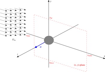
. Figure 1 shows the coordinate system and the geometry adopted for the present work. The Cartesian system passes through the centre of the sphere, the
 $x$
-axis has been chosen parallel to the incoming uniform velocity and the rotation rate vector
 $\unicode[STIX]{x1D74E}$
is aligned with the
 $z$
-axis. The flow is described by the usual time-dependent Navier–Stokes equations:
 $$\begin{eqnarray}\displaystyle & \displaystyle \unicode[STIX]{x1D735}\boldsymbol{\cdot }\boldsymbol{u}=0, & \displaystyle\end{eqnarray}$$
 $$\begin{eqnarray}\displaystyle & \displaystyle \frac{\unicode[STIX]{x2202}\boldsymbol{u}}{\unicode[STIX]{x2202}t}+\boldsymbol{u}\boldsymbol{\cdot }\unicode[STIX]{x1D735}\boldsymbol{u}=-\unicode[STIX]{x1D735}P+\unicode[STIX]{x1D708}\unicode[STIX]{x1D6FB}^{2}\boldsymbol{u}, & \displaystyle\end{eqnarray}$$
 $P\in \mathbb{R}$
is the reduced pressure scalar field,
 $\boldsymbol{u}\in \mathbb{R}^{3}$
is the velocity vector with components
 $\boldsymbol{u}=(u,v,w)$
and
 $\unicode[STIX]{x1D708}$
is the kinematic viscosity.
Perspective view of the computational domain and the frame of reference. This configuration is characterized by a uniform incoming flow
 $U_{\infty }$
and by the sphere angular velocity
 $\unicode[STIX]{x1D74E}$
which is directed along the
 $z$
-axis. The computational domain (dashed lines) extends from
 $x_{inlet}$
to
 $x_{outlet}$
, from
 $y_{down}$
to
 $y_{up}$
and is symmetric in the spanwise direction with a width of
 $z_{lat}$
.

This system of differential equations is completed by boundary conditions at the surface of the sphere
 $\unicode[STIX]{x2202}\mathscr{D}_{sph}$
and a matching condition at infinity, namely
 $$\begin{eqnarray}\displaystyle & \displaystyle \boldsymbol{u}|_{\boldsymbol{r}=\boldsymbol{R}_{sphere}}=\unicode[STIX]{x1D74E}\times \boldsymbol{r}=\unicode[STIX]{x1D74E}\hat{\boldsymbol{e}}_{3}\times \boldsymbol{r},\quad \text{ on }\unicode[STIX]{x2202}\mathscr{D}_{sph}; & \displaystyle\end{eqnarray}$$
 $$\begin{eqnarray}\displaystyle & \displaystyle \boldsymbol{u}\rightarrow \boldsymbol{U}_{\infty }=U_{\infty }\hat{\boldsymbol{e}}_{1},\quad \text{ as }|\boldsymbol{r}|\rightarrow \infty . & \displaystyle\end{eqnarray}$$
 $\unicode[STIX]{x2202}\mathscr{D}_{in}$
and on the lateral sides
 $\unicode[STIX]{x2202}\mathscr{D}_{lat}$
of the computational domain, while a no-traction condition is applied at the outlet surface, namely
 $$\begin{eqnarray}\boldsymbol{n}\boldsymbol{\cdot }(Re^{-1}\unicode[STIX]{x1D735}\boldsymbol{u}-p\boldsymbol{I})|_{x=x_{outlet}}=0,\quad \text{on }\unicode[STIX]{x2202}\mathscr{D}_{out}.\end{eqnarray}$$
The hydrodynamic loads can be obtained by integrating the stress tensor over the sphere surface. In particular, the aerodynamic lift coefficient reads
 $$\begin{eqnarray}C_{L}=\frac{2}{\unicode[STIX]{x1D70C}U_{\infty }^{2}\bar{A}},\quad \text{with }{\mathcal{L}}=\int _{\mathscr{D}_{sph}}[-p\boldsymbol{n}_{y}+\unicode[STIX]{x1D707}(\unicode[STIX]{x1D735}\boldsymbol{u}+\unicode[STIX]{x1D735}\boldsymbol{u}^{T})\boldsymbol{\cdot }\boldsymbol{n}_{y}]\,\text{d}S,\end{eqnarray}$$
where
 $D$
and
 $\bar{A}=\unicode[STIX]{x03C0}D^{2}/4$
are the diameter and the cross-sectional area of the sphere respectively and
 $\boldsymbol{n}$
is the normal vector to the surface of the sphere, with Cartesian components
 $n_{x}$
,
 $n_{y}$
and
 $n_{z}$
.
The dynamics, governed by the incompressible Navier–Stokes equations (2.1), depends on the Reynolds number
 $\mathit{Re}=U_{\infty }D/\unicode[STIX]{x1D708}$
and the dimensionless rotation rate
 $\unicode[STIX]{x1D6FA}=\unicode[STIX]{x1D74E}D/2U_{\infty }$
. The pressure is non-dimensionalized with respect to the dynamic pressure
 $\unicode[STIX]{x1D70C}U_{\infty }^{2}$
and the time with respect to the characteristic time scale
 $U/D$
.
3 Linear stability and sensitivity
We investigate the stability characteristics of the flow past a rotating sphere. The starting point for the global hydrodynamical stability analysis is the assumption that the total flow field
 $[\boldsymbol{u},P]$
only displays small-amplitude deviations
 $[\boldsymbol{u}^{\prime },P^{\prime }]$
with respect to an equilibrium state, i.e. a fixed point, called the base flow
 $[\boldsymbol{U}^{b},P^{b}]$
. Namely,
 $$\begin{eqnarray}\displaystyle & \displaystyle \boldsymbol{u}(x,y,z,t)=\boldsymbol{U}^{b}(x,y,z)+\unicode[STIX]{x1D716}\boldsymbol{u}^{\prime }(x,y,z,t)+O(\unicode[STIX]{x1D716}^{2}), & \displaystyle\end{eqnarray}$$
 $$\begin{eqnarray}\displaystyle & \displaystyle P(x,y,z,t)=P^{b}(x,y,z)+\unicode[STIX]{x1D716}P^{\prime }(x,y,z,t)+O(\unicode[STIX]{x1D716}^{2}), & \displaystyle\end{eqnarray}$$
 $\unicode[STIX]{x1D716}\ll 1$
. The long-term stability features of the flow are then investigated using the decomposition into the classical normal mode form
 $$\begin{eqnarray}\displaystyle & \displaystyle \boldsymbol{u}^{\prime }(x,y,z,t)=\hat{\boldsymbol{u}}(x,y,z)\text{e}^{\unicode[STIX]{x1D70E}t+\text{i}\unicode[STIX]{x1D706}t}, & \displaystyle\end{eqnarray}$$
 $$\begin{eqnarray}\displaystyle & \displaystyle P^{\prime }(x,y,z,t)=\hat{P}(x,y,z)\text{e}^{\unicode[STIX]{x1D70E}t+\text{i}\unicode[STIX]{x1D706}t}, & \displaystyle\end{eqnarray}$$
 $[\hat{\boldsymbol{u}},\hat{P}](x,y,z)$
and by the inherent growth rate
 $\unicode[STIX]{x1D70E}$
and frequency
 $\unicode[STIX]{x1D706}$
. By introducing (3.1) and (3.2) into the Navier–Stokes system (2.1) and neglecting high-order terms, we obtain two different problems: (i) the base-flow problem, which is governed by the time-independent version of (2.1) with boundary conditions (2.2), and (ii) the global stability problem, which reads
 $$\begin{eqnarray}\displaystyle & \displaystyle \unicode[STIX]{x1D735}\boldsymbol{\cdot }\hat{\boldsymbol{u}}=0, & \displaystyle\end{eqnarray}$$
 $$\begin{eqnarray}\displaystyle & \displaystyle (\unicode[STIX]{x1D70E}+\boldsymbol{i}\unicode[STIX]{x1D706})\hat{\boldsymbol{u}}+\boldsymbol{U}_{b}\boldsymbol{\cdot }\unicode[STIX]{x1D735}\hat{\boldsymbol{u}}+\hat{\boldsymbol{u}}\boldsymbol{\cdot }\unicode[STIX]{x1D735}\boldsymbol{U}_{b}=-\unicode[STIX]{x1D735}\hat{P}+\frac{1}{Re}\unicode[STIX]{x1D6FB}^{2}\hat{\boldsymbol{u}}. & \displaystyle\end{eqnarray}$$
This system (3.3), along with the following boundary conditions:
 $$\begin{eqnarray}\displaystyle & \displaystyle \hat{\boldsymbol{u}}|_{\boldsymbol{r}}=\mathbf{0}\quad (\text{on the sphere surface }\unicode[STIX]{x2202}\mathscr{D}_{sph}); & \displaystyle\end{eqnarray}$$
 $$\begin{eqnarray}\displaystyle & \displaystyle \hat{\boldsymbol{u}}=\mathbf{0}\quad (\text{on the lateral sides }\unicode[STIX]{x2202}\mathscr{D}_{lat}\text{ and at the inlet surface }\unicode[STIX]{x2202}\mathscr{D}_{in}); & \displaystyle\end{eqnarray}$$
 $$\begin{eqnarray}\displaystyle & \displaystyle \boldsymbol{n}\boldsymbol{\cdot }(Re^{-1}\unicode[STIX]{x1D735}\hat{\boldsymbol{u}}-\hat{p}\boldsymbol{I})|_{x=x_{outlet}}=0\quad (\text{on the outlet surface }\unicode[STIX]{x2202}\mathscr{D}_{out}); & \displaystyle\end{eqnarray}$$
 $\unicode[STIX]{x1D70E}<0$
, the flow is linearly stable, while when
 $\unicode[STIX]{x1D70E}>0$
, the perturbation grows exponentially in time.
In order to locate the core of the instability and to describe the features of the inherent flow, we rely on the concept of a wavemaker used in stability analysis (Giannetti & Luchini Reference Giannetti and Luchini2007). Following the recent review by Luchini & Bottaro (Reference Luchini and Bottaro2014), we use a linear adjoint-based approach to determine this region. The resulting sensitivity tensor is given by
 $$\begin{eqnarray}\unicode[STIX]{x1D64E}(x,y,z)={\displaystyle \frac{\hat{\boldsymbol{u}}^{\dagger }(x,y,z)\hat{\boldsymbol{u}}(x,y,z)}{\displaystyle \int _{\mathscr{D}}\hat{\boldsymbol{u}}^{\dagger }(x,y,z)\boldsymbol{\cdot }\hat{\boldsymbol{u}}(x,y,z)\,\text{d}V}},\end{eqnarray}$$
where the adjoint fields
 $(\hat{u} ^{\dagger },\hat{p}^{\dagger })$
are obtained using the generalized Lagrange identity (Ince Reference Ince1926)
 $$\begin{eqnarray}\displaystyle & \displaystyle \unicode[STIX]{x1D735}\boldsymbol{\cdot }\hat{\boldsymbol{u}}^{\dagger }=0, & \displaystyle\end{eqnarray}$$
 $$\begin{eqnarray}\displaystyle & \displaystyle -(\unicode[STIX]{x1D70E}+\boldsymbol{i}\unicode[STIX]{x1D706})\hat{\boldsymbol{u}}^{\dagger }+\boldsymbol{U}_{b}\boldsymbol{\cdot }\unicode[STIX]{x1D735}\hat{\boldsymbol{u}}^{\dagger }-\unicode[STIX]{x1D735}\boldsymbol{U}_{b}\boldsymbol{\cdot }\hat{\boldsymbol{u}}^{\dagger }=-\unicode[STIX]{x1D735}\hat{p}^{\dagger }-\frac{1}{Re}\unicode[STIX]{x1D6FB}^{2}\hat{\boldsymbol{u}}^{\dagger }. & \displaystyle\end{eqnarray}$$
4 Numerical methods
The results presented in this work are found using two different codes: (i) a combined finite-difference second-order immersed-boundary multigrid (IBM) code and (ii) the spectral finite-element software Nek5000 (Tufo & Fischer Reference Tufo and Fischer1999).
The finite-difference (IBM) code is based on a classical second-order conservative discretization of the Navier–Stokes equations on a staggered non-uniform Cartesian mesh. In order to achieve higher accuracy and save computational time, a grid clustering near the sphere is used. The boundary conditions on the sphere are imposed through a second-order-accurate immersed-boundary scheme, in which the stencil of the finite-difference operators near the body is modified using an appropriate interpolation–extrapolation procedure. More precisely, the interpolation is performed using the point closest to the body surface (which can be either an internal or an external point) and the following point on the exterior of the sphere. The interpolation is performed in either the streamwise or the transverse direction according to which one is closest to the local normal. Linear or quadratic reconstruction was used and tested, leading in both cases to a global second-order accuracy. The discretized three-dimensional problem is then solved by using an in-house linear multigrid solver coupled with a Newton global linearization (Trottenberg, Oosterlee & Schüller Reference Trottenberg, Oosterlee and Schüller2001). In order to obtain good convergence in the presence of highly stretched grids, an alternating collective line Gauss–Seidel (CLGS) smoother was used. This relaxation procedure considers a line of computational cells as a main block of a Gauss–Seidel-type iteration, which leads to a banded six-diagonal system of linear equations to be solved at each subiteration of the multigrid algorithm. This procedure is the line version of the more classical block Vanka smoother (Vanka Reference Vanka1986) and has been used with a classical
 $V$
cycle (Trottenberg et al.
Reference Trottenberg, Oosterlee and Schüller2001). In our version, the matrix entries are calculated by a local linearization of the governing equations. More details on the characteristics of this kind of smoother can be found in Feldman & Gelfgat (Reference Feldman and Gelfgat2009). The discretization of the convective terms can be problematic since the classical second-order centred discretization is not h-elliptic and can lead to a severe degradation and failure of the iterative procedure. In our code, the convective terms are discretized with a standard first-order upwind discretization, while second-order accuracy is recovered through a standard deferred correction procedure based on classical centred discretization implemented at the smoother level. The immersed-boundary technique with a quadratic interpolation is applied only on the finest level, while, for simplicity, at coarser levels, a stair-step geometry is considered. This procedure does not alter the overall convergence speed of the multigrid algorithm and considerably simplifies the coding and the computational time. Textbook multigrid efficiency (Trottenberg et al.
Reference Trottenberg, Oosterlee and Schüller2001) is achieved far from the bifurcation thresholds. As for all iterative procedures close to a transition threshold, a severe degradation of the performance is obtained. This is due to the existence of a limited number of eigenvalues of the iteration matrix moving and crossing the imaginary line: in this situation the whole iterative procedure diverges. In order to avoid this problem, we used a stabilizing procedure able to significantly accelerate the convergence of our multigrid. In fact, one of the original ingredients of our code is the ability to perform the base-flow and stability computations simultaneously (Luchini, Giannetti & Pralits Reference Luchini, Giannetti, Pralits, Leweke, Meneghini and Williamson2007). At each iteration, the approximate knowledge of the leading eigenvalues is used to accelerate the convergence of the base flow. While this is not particularly important when we are far from the critical Reynolds number, this strategy becomes essential close to the critical point and in the unstable region, where the convergence of classical multigrid algorithms is slowed down by the presence of slowly decaying or unstable modes. In such conditions, classical smoothers (such as Jacobi, Gauss–Seidel or Vanka type) are not able to suppress the high-frequency content of the error, leading in many cases to divergence. In order to track the bifurcation, in these situations, complex algorithms have to be implemented. An example is offered by the RPM method, in which the computational space is divided into the direct sum of a stable and an unstable subspace. In the stable subspace, the algorithm uses classical smoothers, while a Newton iteration is adopted in the small unstable subspace. This algorithm is, however, very complex to code up and difficult to insert in an already existing code. For the present investigation, in the attempt to accelerate the convergence of the base flow and perform the stability analysis close to the critical point, we have adopted a different approach in which a subspace iteration method based on an approximate inverse (obtained through the multigrid iteration) of the linearized Navier–Stokes operator is adopted to extract and filter out the slow-converging components of the solution (leading modes). Details of the algorithm can be found in Luchini et al. (Reference Luchini, Giannetti, Pralits, Leweke, Meneghini and Williamson2007).
The second code used for the present analysis is the spectral element code Nek5000. In this software, the velocity vector field and the pressure scalar field are discretized onto
 $P_{N}{-}P_{N-2}$
spectral elements using Lagrange orthogonal polynomials in the Gauss–Lobatto–Legendre (GLL) nodes. The temporal discretization for the momentum equation is achieved by using a semi-implicit splitting scheme. The resulting algorithm solves the convective, viscous and pressure problems. An overlapping Schwarz method (Fischer Reference Fischer1997) is adopted to solve the latter two elliptic problems.
The immersed-boundary multigrid code is particularly useful to track the neutral curves and the imperfect bifurcation. For stability computations (where just a few leading modes are needed), this approach is considerably faster than the classical time-stepper approach (Bagheri et al. Reference Bagheri, Åkervik, Brandt and Henningson2009a ) used with Nek5000, in which the base flow is first computed and then an Arnoldi algorithm implemented in the ParPACK package is used in conjunction with the time-resolved solution of the linearized Navier–Stokes equations. For this reason, most of the parametric computations have been performed with the multigrid code. Nek5000, on the other hand, uses a spectral element method (SEM) and can achieve higher spatial accuracy. Therefore, this code has been used to cross-validate the results and their accuracy. Moreover, it was used to perform time-resolved computations and verify the validity of the linear stability results. We discuss in § 4.1 the details of the methodology adopted to compute the base flows in supercritical conditions with Nek5000. Due to the high degree of optimization and parallel scalability, this code is really efficient when an accurate time-resolved solution of the unsteady Navier–Stokes equations is needed. Taking advantage of these characteristics, the two codes have been used in a complementary way to cross-validate the results and reduce the computational effort.
4.1 Computation of base flows near the bifurcations
Within a time-stepper approach, the 3D steady base-flow solution can be obtained by simply integrating the time-dependent Navier–Stokes equations (2.1) over a long time interval when the flow is in subcritical conditions, i.e. before the occurrence of a bifurcation. However, if the Reynolds number exceeds the instability threshold, we cannot use a simple time integration to compute the unstable steady base flow that is required for the global stability analysis. It is, therefore, necessary to use a stabilizing numerical procedure able to retrieve the unstable reference state. In the case of low-dimensional systems, on one hand, there exist several continuation and bifurcation packages like AUTO (Doedel Reference Doedel1986) or CONTENT (Kuznetsov & Levitin Reference Kuznetsov and Levitin1996) based on direct solvers for the linear algebraic systems and eigenvalue problems involved in the computations. On the other hand, since the discretization of a full three-dimensional problem often leads to a very large discrete system, the extension to high-dimensional problems is not straightforward.
It should be noted that computation of the steady solution using a Newton algorithm, which is the most commonly used method in global stability studies of 2D flows, is not suitable here, as it necessitates a matrix inversion which would require too much memory and time in a 3D case. An alternative, however, would be to adopt a Krylov-subspace method like the classical GMRES (Saad Reference Saad2003). Other approaches can be found in the literature. In Åkervik et al. (Reference Åkervik, Brandt, Henningson, Hoepffner, Marxen and Schlatter2006), for instance, the authors managed to reach the steady state by damping the unstable frequencies using a dissipative relaxation term proportional to the high-frequency content of the velocity fluctuation field. Shroff & Keller (Reference Shroff and Keller1993), instead, were able to compute unstable states by using a projection onto the small unstable subspace coupled with a Newton procedure.
As discussed in the previous section, the base flow is obtained in two different ways. For the Cartesian multigrid method, details have been discussed above. For the Nek5000 code, we adopt a novel efficient algorithm (Citro et al.
Reference Citro, Luchini, Giannetti and Auteri2016), inspired by the Krylov-subspace methods, to compute unstable steady states of the inherent dynamical system. This method, like GMRES, is based on the minimization of the residual norm at each integration step. It allows us to obtain the unstable steady field by correcting the new iteration of the numerical procedure using a linear combination of previous fields. The key steps of this procedure can be found in appendix A of Citro et al. (Reference Citro, Giannetti, Luchini and Auteri2015). However, we tested our algorithm in computing the flow past a circular cylinder. In this case, the maximum difference between the base flow computed using our algorithm and the classical Newton–Raphson method is less than
 $10^{-10}$
.
4.2 Convergence analysis and validation
The computational domain is chosen to be a large rectangular box surrounding the bluff body (see figure 1). In our case, it extends from
 $x_{inlet}$
to
 $x_{outlet}$
, from
 $y_{down}$
to
 $y_{up}$
and is symmetric in the
 $z$
direction with a width of
 $z_{lat}$
.
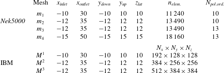
The different meshes used to validate our numerical simulations. Nek5000:
 $n_{elem.}$
is the total number of spectral elements inside the computational domain;
 $N_{pol.ord.}$
is the polynomial order adopted for the spatial discretization.
 $IBM$
code:
 $N_{x}$
,
 $N_{y}$
,
 $N_{z}$
are respectively the total number of points in the
 $x$
,
 $y$
and
 $z$
directions.

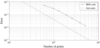
Truncation error (
 $L_{2}$
norm) as a function of the number of points for the finite-difference second-order immersed-boundary multigrid code. The solution on a grid of
 $1024\times 512\times 512$
is assumed as the reference solution. In particular, we report here the number of points in the
 $x$
direction,
 $N_{x}$
; the other two directions are characterized by
 $N_{y}=N_{z}=0.5N_{x}$
. The dashed line represents the theoretical second-order scaling of the error.

Table 1 shows the details of the several meshes used for the analysis (for both the IBM and the SEM code). The adopted grids present a clustering of points near the sphere surface and are symmetrically located with respect to the plane (
 $x$
–
 $y$
). For the Cartesian IBM code, Roberts stretching transformations (Tannehill, Anderson & Pletcher Reference Tannehill, Anderson and Pletcher1997, pp. 336–337) are used to smoothly cluster the points close to the sphere centre. A similar approach has been successfully used in Giannetti & Luchini (Reference Giannetti and Luchini2007).
In the case of Nek5000, the domain is discretized into hexahedral elements, which are deformed by isoparametric mappings. Within each element, the unknown is represented in local Cartesian coordinates by tensor-product Lagrange polynomials of degree
 $N_{pol.ord.}$
(and
 $N_{pol.ord.}-2$
for the pressure field). The upper part of table 1 shows the characteristics of these meshes. The grids adopted in the immersed-boundary calculations are also reported in the same table. In order to validate our numerical methods, we performed several tests to study the effects of the resolution and of the size of the computational domain. A grid convergence analysis was performed for the new immersed-boundary code. Figure 2 depicts the evolution of the error as a function of the number of points adopted in the discretization (in the
 $x$
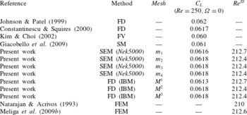
direction). We found perfect agreement between the second-order theoretical scaling of the error and the evolution of the error computed by our multigrid code. Furthermore, a validation analysis has been carried out in order to select the best grid in terms of speed and accuracy. Table 2 shows the comparison between the results obtained by the present numerical approaches and the dedicated literature. We found small changes in the lift coefficient
 $C_{L}$
and in the critical Reynolds number
 $Re^{SS}$
for the first bifurcation. Thus, for efficiency reasons, we chose the meshes
 $m_{2}$
and
 $M^{2}$
to compute all of the results documented in the present work.
Validation of the present numerical approaches. In particular, we compare the lift coefficient
 $C_{L}$
and the critical Reynolds number for the first bifurcation
 $\mathit{Re}^{SS}$
with values reported in the literature. (FD
 $=$
finite-difference method, SEM
 $=$
spectral element method, FV
 $=$
finite-volume method, FEM
 $=$
finite-element method).

Flow past a sphere immersed in a uniform stream: contour plot of the pressure fields for several flow conditions. The white lines represent the streamlines of the flow. The fixed sphere case (
 $\unicode[STIX]{x1D6FA}=0.0$
) is depicted using two cases: (a) axisymmetric state at
 $\mathit{Re}=200$
and (b) asymmetric flow at
 $\mathit{Re}=275$
(onset of mode I without rotation). Furthermore, we select four cases to show the spatial structure of the flow for mode I: (c)
 $\unicode[STIX]{x1D6FA}=0.01$
,
 $\mathit{Re}=200$
, (d)
 $\unicode[STIX]{x1D6FA}=0.01$
,
 $\mathit{Re}=270$
, (e)
 $\unicode[STIX]{x1D6FA}=0.2$
,
 $\mathit{Re}=200$
, (f)
 $\unicode[STIX]{x1D6FA}=0.2$
,
 $\mathit{Re}=240$
; and two cases for mode II: (g)
 $\unicode[STIX]{x1D6FA}=0.9$
,
 $\mathit{Re}=200$
, (h)
 $\unicode[STIX]{x1D6FA}=0.9$
,
 $\mathit{Re}=270$
.

5 Results
5.1 Base flow
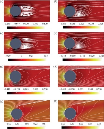
Figure 3 displays the typical shape of the base flow through contours of the pressure field and streamlines in the lateral (
 $x$
–
 $y$
) mid-plane (
 $z=0$
). First of all, we review the case without rotation
 $(\unicode[STIX]{x1D6FA}=0)$
. For
 $Re<Re^{SS}=212$
(figure 3
a), the base flow remains axisymmetric, and the structure is the same in every transverse plane. This flow state consists of a toroidal recirculation region with closed streamlines. In topologic terms, the flow along the sphere is characterized by two detachment points in the symmetry plane, plus a central reattachment point, while the flow in the wake is characterized by two stable foci and one saddle point.
Above this threshold, intrinsic wake dynamics leads to a spontaneous symmetry breaking, the resulting state displaying only a planar symmetry with respect to an arbitrary transverse plane (which is taken here as the (
 $x$
–
 $y$
) plane for consistency with the results in the rotating case). When observed in this symmetry plane, the recirculation region is asymmetric, one of the vortical structures becoming stronger than the other one (see figure 3
b for
 $Re=275$
). One can also note that the streamlines in the symmetry plane are no longer closed, but are spiralling towards a converging focus in the upper half and outwards from a diverging focus in the lower half. As described in detail by Johnson & Patel (Reference Johnson and Patel1999), this feature indicates a three-dimensional flow along the toroidal structure, with streamlines diverging in the third direction from the upper focus and converging towards the lower one. It should be noted also that the central reattachment point is shifted upwards, while the locations of the two detachment points are weakly modified. Finally, the isocontours indicate that pressure is larger near the upper part of the sphere surface, which results in a negative lift.
In the presence of rotation, the axisymmetry of the flow is always broken and replaced by a planar symmetry with respect to the transverse plane (
 $x$
–
 $y$
) perpendicular to the rotation
 $z$
-axis. Figure 3(c) displays the base flow for a weak rotation (
 $\unicode[STIX]{x1D6FA}=0.01$
) and low Reynolds number
 $\mathit{Re}=200$
. Compared with the non-rotating case, one can observe that the location of the detachment point is shifted downstream in the lower half and upstream in the upper half. As a consequence, the recirculation region becomes asymmetric, the lower structure becoming stronger than the upper one. Overall, the resulting wake is very similar to the one resulting from the bifurcation at
 $Re^{SS}$
in the non-rotating case, with non-closed streamlines indicating divergence/convergence of the flow in the perpendicular direction. The effect of rotation on the pressure is also to decrease the pressure on the lower side of the sphere and to increase it on the upper side. This is in accordance with the classical explanation of the Magnus effect, and results in a net negative lift force. Figure 3(d) displays the base flow for the same weak rotation rate (
 $\unicode[STIX]{x1D6FA}=0.01$
) and higher Reynolds number
 $\mathit{Re}=270$
. In this case the recirculation region becomes strongly asymmetric. We can interpret this as a superposition of the two previous effects: the Magnus effect due to rotation and the intrinsic wake mechanism responsible for the symmetry breaking in the absence of rotation reinforcing each other.
The base-flow lift
 $C_{L}$
as a function of the Reynolds number
 $\mathit{Re}$
for various values of
 $\unicode[STIX]{x1D6FA}$
.

As the rotation rate is further increased, the regions with spiralling streamlines in the upper and lower parts of the wake disappear, as already found by Giacobello et al. (Reference Giacobello, Ooi and Balachandar2009). This is exemplified by figure 3
 $(e)$
, which displays the base flow for a moderate rotation (
 $\unicode[STIX]{x1D6FA}=0.2$
) and Reynolds number
 $\mathit{Re}=200$
. It should be noted that the topology of the flow becomes different and simpler compared with the previous case. Considering the flow along the sphere, there is now a single detachment point located on the upper half of the sphere instead of a pair of detachment points and a central reattachment point. Considering the flow in the wake, the two foci and the saddle point have also vanished. Consequently, the recirculation becomes fully open. As can be seen in 3(f) for
 $\mathit{Re}=240$
, increasing the Reynolds number does not strongly modify the structure of the flow. In both of these plots we still observe that the pressure is decreased on the lower side of the sphere and increased on the upper side. Again, in accordance with the classical explanation of the Magnus effect, this results in a net negative lift force. It should be noted that although the plots only depict the flow in the symmetry plane, the streamlines give an indication of the three-dimensionality of the flow. Namely, in the vicinity of the upper detachment point, the tightening of the streamlines indicates divergence in the perpendicular direction, while in the lower part of the wake, the spreading of the streamlines indicates convergence in the perpendicular direction.
Figures 3(g) and 3(h) display the case of a larger rotation rate,
 $\unicode[STIX]{x1D6FA}=0.9$
, with
 $\mathit{Re}=200$
and
 $\mathit{Re}=270$
respectively. We can note that the open recirculation region originating from the detachment point on the upper half of the sphere becomes more open and more intense with respect to the previous cases. The base-flow results obtained for subcritical values of the parameters are in perfect agreement with the simulations by Giacobello et al. (Reference Giacobello, Ooi and Balachandar2009). In fact, the streamline patterns presented here (in subcritical conditions) are very similar to the ones reported in figure 8 of Giacobello et al. (Reference Giacobello, Ooi and Balachandar2009).
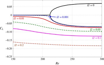
Figure 4 details the lift force exerted upon the sphere as a function of the Reynolds number, for several values of the rotation rate. Without rotation (
 $\unicode[STIX]{x1D6FA}=0$
), one recovers the picture already described, namely zero lift below
 $Re^{SS}=212$
and a bifurcation towards a non-zero lift situation above this value. For
 $\unicode[STIX]{x1D6FA}>0$
, the lift is always negative and of larger magnitude than in the non-rotating case. This is consistent with the fact that the intrinsic wake dynamics and the Magnus effect reinforce each other to build the lift force, as explained previously.
Finally, in this figure, the curves corresponding to the lowest values of
 $\unicode[STIX]{x1D6FA}$
approach the curves of the non-rotating case, except in the vicinity of
 $Re^{SS}$
where a continuous transition is observed. This feature is linked to the fact that the pitchfork bifurcation existing in the absence of rotation actually becomes an imperfect bifurcation in the case of slow rotation. Accordingly, in the vicinity of the threshold, one expects to encounter other equilibrium solutions lying on a separate branch disconnected from the one considered here. Such solutions were actually effectively found, but they turned out to always be unstable. Hence, we prefer not to document these additional solutions in the present section. The imperfect bifurcation for small rotation will be reconsidered in detail in § 6.
(a) Neutral stability curves for the three-dimensional flow past a transversely rotating sphere: (*) mode I; (○) mode II. We report also DNS results provided by Giacobello et al. (Reference Giacobello, Ooi and Balachandar2009), Kim (Reference Kim2009) and Poon et al. (Reference Poon, Ooi, Giacobello and Cohen2010): (▫) stable simulations; (▵) unstable DNS (they reported the existence of a saturated limit cycle). (b) Strouhal numbers for mode I and II.

5.2 Global stability
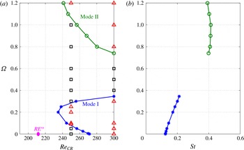
We now detail the results of the global linear stability analysis outlined in § 5.1. The main outcome of this study is depicted in figure 5(a), which displays the thresholds for linear instability in the
 $Re/\unicode[STIX]{x1D6FA}$
parameter plane. We observe the existence of two distinct regions. The first region exists for moderate values of the rotation (
 $\unicode[STIX]{x1D6FA}<0.4$
). This mode, called ‘mode I’ in the following, is one that exists in the non-rotating case (
 $\unicode[STIX]{x1D6FA}=0$
). As can be observed, small rotation has a destabilizing effect: the threshold Reynolds number decreases from
 $272$
in the non-rotating case to
 $\mathit{Re}_{cr}^{mode\,I}=235$
for
 $\unicode[STIX]{x1D6FA}=0.2$
. However, increasing the rotation again has the opposite effect: in the range
 $\unicode[STIX]{x1D6FA}=[0.2,0.4]$
, the value of the critical Reynolds number becomes larger than
 $300$
. We suggest that these trends are related to the transition in the wake flow topology. In particular, when
 $0.0\leqslant \unicode[STIX]{x1D6FA}\leqslant 0.2$
, the recirculation bubble is asymmetric and one of the recirculation regions grows; this modification to the base-flow structure destabilizes the flow past rotating spheres for a mild rotation. On the other hand, when
 $\unicode[STIX]{x1D6FA}>0.2$
, the recirculation bubble disappears and the flow, as a consequence, becomes more stable as the rotation rate increases.
The second region of instability occurs for larger rotations, namely
 $\unicode[STIX]{x1D6FA}>0.7$
in the range of
 $Re$
considered, and is related to the existence of a second unstable branch. For this second mode, denoted ‘mode II’, the effect of rotation is destabilizing as the threshold Reynolds number decreases as
 $\unicode[STIX]{x1D6FA}$
is further increased.
In figure 5(a), we have also displayed with symbols the DNS results of Kim (Reference Kim2009) and Poon et al. (Reference Poon, Ooi, Giacobello, Iaccarino and Chung2014) for
 $Re=250$
and 300. As can be seen, these results are in excellent agreement with ours, since all of their unsteady simulations fall inside the regions we found to be linearly unstable, while all of their steady simulations fall in the stable one.
Figure 5(b) shows the effect of
 $\unicode[STIX]{x1D6FA}$
on the Strouhal number associated with the eigenfrequency of the unstable global modes. We note that
 $St$
displays a relatively linear dependence on
 $\unicode[STIX]{x1D6FA}$
for mode I, while it is almost constant for mode II. Thus, we can conclude that, for mode II, the rotation rate
 $\unicode[STIX]{x1D6FA}$
weakly affects the Strouhal number which is approximatively
 $0.4$
. Our results agree well with those reported by Giacobello et al. (Reference Giacobello, Ooi and Balachandar2009), Kim (Reference Kim2009) and Poon et al. (Reference Poon, Ooi, Giacobello and Cohen2010) using DNS.
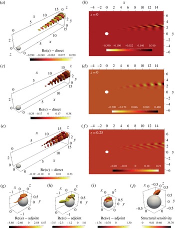
Mode I (see figure 5). (a,c,e) Isosurfaces of direct streamwise
 $\hat{u}$
, transverse
 $\hat{v}$
and spanwise
 ${\hat{w}}$
velocity field. (b,d) Contour plots of the inherent component in the symmetry plane and (f) in the plane
 $z=0.25$
. The adjoint mode I is also depicted in (g,h) and (i) by using isosurfaces. (j) The resulting structural sensitivity field. Parameter settings:
 $\unicode[STIX]{x1D6FA}=0.2$
,
 $\mathit{Re}=235$
.

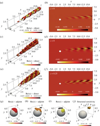
Figure 6(a–f) shows the spatial structure of the velocity field of direct mode I. This global mode is dominated by axially extended streamwise velocity disturbances located downstream of the sphere. It should be noted that the
 $u$
and
 $v$
components are symmetric with respect to the
 $(x,y)$
plane while the
 $w$
component is antisymmetric (figure 6
a,c,e). This means that the unsteady mode, which emerges from this instability, respects the planar (
 $x$
–
 $y$
) symmetry of the underlying base flow. This fact is consistent with classical results for a non-rotating sphere. Figure 6(g–i) depicts the spatial distribution of the adjoint field. It should be noted that the latter is strongly localized near the surface of the sphere, more specifically in the upper part of the sphere where the shear is largest due to opposite rotation. We underline here that the adjoint field can be considered as a Green’s function for the receptivity of the corresponding global mode (Giannetti & Luchini Reference Giannetti and Luchini2007). In fact, the amplitude of the instability mode is provided by the scalar product of the adjoint with any forcing function and/or initial condition. Mode I can therefore be most efficiently triggered in the near wake of the bluff body. In order to characterize the instability mechanism, we also performed a structural sensitivity analysis. The latter region, depicted in figure 6(l), is localized in a near-wake region of the sphere, across the surface separating the outer flow from the wake region. From these observations we may infer that (i) the region responsible for this instability (wavemaker) is localized in the recirculation region behind the sphere and (ii) the instability is mostly receptive to perturbations near the surface of the sphere.
The same as figure 6. Parameter settings:
 $\unicode[STIX]{x1D6FA}=0.9$
at
 $\mathit{Re}=270$
.

Figure 7 shows the spatial distribution of the direct and adjoint mode II and the resulting structural sensitivity. The structure of this direct global mode is again characterized by spatial oscillations downstream of the sphere. We notice that mode II presents faster spatial oscillations than mode I but presents a similar spatial shape. This means that like mode I, mode II preserves the planar symmetry of the base flow. As a result, the oscillating flow resulting from these unstable modes is not expected to display oscillations with respect to the mean plane. Our results agree well with the DNS results provided by Kim (Reference Kim2009).
The adjoint mode II is depicted in figure 7(g–i). It is still localized near the sphere surface. We found that the region of maximum receptivity for shedding mode II is still localized near the sphere surface and is stronger than that of mode I.
On the other hand, the structural sensitivity indicates that the region responsible for instability (the ‘wavemaker’) is also localized in a region of strong shear near the sphere surface. This finding agrees well with the conclusion of Giacobello et al. (Reference Giacobello, Ooi and Balachandar2009, § 3.3) that suggested a Kelvin–Helmholtz instability of the shear layer as the instability mechanism.
We note that it is possible to use the previous results to develop an effective passive control strategy for rotating sphere flows. Pralits et al. (Reference Pralits, Brandt and Giannetti2010) showed that a small control body can be placed in order to suppress the vortex shedding in the wake of a rotating circular cylinder. Their computations illustrated how a technique based on a structural sensitivity analysis of the governing equations can be used to design efficient control strategies for the vortex shedding behind bluff bodies. In our case, we note that the wavemakers of modes I and II are close to each other. Therefore, there could be a possibility of controlling both modes simultaneously by using a simple strategy.
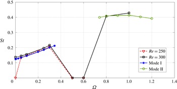
Finally, we compare the Strouhal number computed in the present investigation with vortex shedding frequencies obtained by Giacobello et al. (Reference Giacobello, Ooi and Balachandar2009). Figure 8 shows that, in the range of rotation rates investigated here, the Strouhal number of a fully developed saturated limit cycle is very similar to the value computed by using the eigenfrequency of the unstable global mode I or II.
Comparison between the Strouhal number computed by using the eigenfrequency of modes I and II and the DNS results reported by Giacobello et al. (Reference Giacobello, Ooi and Balachandar2009) for
 $\mathit{Re}=250$
and
 $\mathit{Re}=300$
.

6 The case of slow rotation
As recalled in the introduction, in the non-rotating case, the flow around a sphere experiences a pitchfork bifurcation at
 $Re=Re^{SS}=212.4$
, which leads from an axisymmetric state with zero lift to a mirror-symmetric state with non-zero lift. To investigate the nature of such bifurcations, and in particular their supercritical or subcritical nature, a usual and straightforward extension of the global stability approach used in the previous section is to perform a weakly nonlinear development in terms of the distance to the threshold.
A general methodology to tackle such weakly nonlinear problems, as well as a numerical method based on finite elements, was introduced by Sipp & Lebedev (Reference Sipp and Lebedev2007) for the case of a 2D cylinder and adapted to 3D objects by Meliga, Chomaz & Sipp (Reference Meliga, Chomaz and Sipp2009a ) and Meliga et al. (Reference Meliga, Chomaz and Sipp2009b ). This methodology is now routinely used in our teams for various problems of fixed (Tchoufag et al. Reference Tchoufag, Assemat, Fabre and Meliga2011) or moving (Tchoufag, Fabre & Magnaudet Reference Tchoufag, Fabre and Magnaudet2014b ; Fabre et al. Reference Fabre, Tchoufag, Citro, Giannetti and Luchini2016) objects of various geometries.
The purpose of the present section is to repeat this calculation for the case of a sphere and to extend it to include the effect of a weak rotation. We will show that the approach directly leads to an amplitude equation describing an imperfect bifurcation, in good accordance with the numerical results obtained by using the IBM code previously described.
6.1 Weakly nonlinear approach
Following Meliga et al. (Reference Meliga, Chomaz and Sipp2009a
), we pose
 $\unicode[STIX]{x1D716}^{2}=1/Re^{SS}-1/Re$
and assume this parameter to be small. The flow is thus expanded in terms of this parameter as follows:
 $$\begin{eqnarray}\boldsymbol{q}=[\boldsymbol{u},p]=\boldsymbol{q}_{0}+\unicode[STIX]{x1D716}\boldsymbol{q}_{1}+\unicode[STIX]{x1D716}^{2}\boldsymbol{q}_{2}+\unicode[STIX]{x1D716}^{3}\boldsymbol{q}_{3}+\cdots \,.\end{eqnarray}$$
In order to introduce the effect of rotation in the method, we also have to assume that the rotation is small. Since in the non-rotating case the amplitude equation derived in Meliga et al. (Reference Meliga, Chomaz and Sipp2009a
) arises from the resolution of the problem at order
 $\unicode[STIX]{x1D716}^{3}$
, we anticipate that
 $\unicode[STIX]{x1D74E}$
has to be of the same order of magnitude, so that we set
 $$\begin{eqnarray}\unicode[STIX]{x1D74E}=\unicode[STIX]{x1D716}^{3}\unicode[STIX]{x1D74E}_{0},\end{eqnarray}$$
where
 $\unicode[STIX]{x1D74E}_{0}$
is the rescaled rotation rate of order one.
Following the standard weakly nonlinear expansion for such flows (Sipp & Lebedev Reference Sipp and Lebedev2007; Meliga et al.
Reference Meliga, Chomaz and Sipp2009a
), we rely on a multi-time scale technique and assume
 $\unicode[STIX]{x1D70F}=\unicode[STIX]{x1D716}^{2}t$
, where
 $\unicode[STIX]{x1D70F}$
and
 $t$
are respectively the slow and fast time scales. Injection of this decomposition into the governing equations (2.1) along with the boundary conditions (2.2) leads to various problems to be solved for
 $Re=Re^{SS}$
at different orders
 $\unicode[STIX]{x1D716}^{j}$
, with
 $j=0,1,2,3,\ldots .$
-
(i) At order
 $\unicode[STIX]{x1D716}^{0}$
, we obtain the nonlinear problem governing
$\boldsymbol{q}_{0}$
, the axisymmetric base flow with no rotation.
-
(ii) At order
$\unicode[STIX]{x1D716}$
, we obtain a linear problem which can be written in a symbolic way as
${\mathcal{L}}\boldsymbol{q}_{1}=0$
. Since we are at the threshold
$Re^{SS}$
, this equation has non-trivial solution with azimuthal wavenumbers
$\pm 1$
(the marginal eigenmodes). The solution at this order is thus a linear combination of the global modes at
$Re=Re^{SS}$
, and is taken as (6.3)where
$$\begin{eqnarray}\boldsymbol{q}_{1}=\hat{A}(\unicode[STIX]{x1D70F})\hat{\boldsymbol{q}}(r,x)\text{e}^{\text{i}\unicode[STIX]{x1D719}}+\text{c.c.},\end{eqnarray}$$
$\hat{\boldsymbol{q}}$
is the eigenvector of the azimuthal wavenumber
$(m=+1)$
and
$\hat{A}$
is a complex amplitude that depends on the slow time scale. It should be noted that the eigenvector
$\hat{\boldsymbol{q}}$
can be normalized so that the real and imaginary parts of the amplitude
$A$
correspond to the
$y$
and
$z$
components of the lift (see Fabre et al.
Reference Fabre, Auguste and Magnaudet2008).
-
(iii) At order
$\unicode[STIX]{x1D716}^{2}$
, the solution contains base-flow viscous corrections due the departure from
$Re^{SS}$
as well as quadratic terms resulting from the self-interactions of the global mode. Using the notations of Meliga et al. (Reference Meliga, Chomaz and Sipp2009a
), this reads as (6.4)
$$\begin{eqnarray}\boldsymbol{q}_{2}=\boldsymbol{q}_{\unicode[STIX]{x1D6FF}}+\boldsymbol{q}_{AA\ast }|A|^{2}+(\boldsymbol{q}_{AA}A^{2}\text{e}^{2\text{i}\unicode[STIX]{x1D719}}+\text{c.c.}).\end{eqnarray}$$
-
(iv) At order
$\unicode[STIX]{x1D716}^{3}$
, one obtains a linear problem which can be written in a symbolic way as follows: (6.5)where
$$\begin{eqnarray}\unicode[STIX]{x2202}_{t}\boldsymbol{q}_{3}+(\unicode[STIX]{x2202}_{\unicode[STIX]{x1D70F}}A\hat{\boldsymbol{q}}\text{e}^{\text{i}\unicode[STIX]{x1D719}}+\text{c.c.})={\mathcal{N}}(\boldsymbol{q}_{2},\boldsymbol{q}_{1})+{\mathcal{L}}\boldsymbol{q}_{3},\end{eqnarray}$$
${\mathcal{N}}(\boldsymbol{q}_{2},\boldsymbol{q}_{1})$
represents the nonlinear interaction between the solutions at the two previous orders, and
${\mathcal{L}}$
is the same linear operator as for the problem at order one. This problem is again similar to the case of Meliga et al. (Reference Meliga, Chomaz and Sipp2009a
), except for the fact that
$\boldsymbol{q}_{3}$
has to verify the boundary condition corresponding to a steady rotation, namely (6.6)As the linear operator governing the system (6.5) is singular, the usual procedure to remove the secular terms consists of taking a scalar product of the forcing terms with the adjoint of the problem. This yields a single differential equation for the amplitude
$$\begin{eqnarray}\boldsymbol{u}_{3}=\unicode[STIX]{x1D74E}_{0}\boldsymbol{z}\times \boldsymbol{r}.\end{eqnarray}$$
$A$
, with the form (6.7)where
$$\begin{eqnarray}\frac{\unicode[STIX]{x2202}A}{\unicode[STIX]{x2202}t}=\unicode[STIX]{x1D706}\unicode[STIX]{x1D716}^{2}A-\unicode[STIX]{x1D707}\left|A\right|^{2}A+a\unicode[STIX]{x1D74E},\end{eqnarray}$$
$\unicode[STIX]{x1D706}$
,
$\unicode[STIX]{x1D707}$
and
$a$
are all real. Here, the coefficients
$\unicode[STIX]{x1D706}$
and
$\unicode[STIX]{x1D707}$
contain the effect of the forcing terms corresponding to the viscous correction (
$\boldsymbol{q}_{\unicode[STIX]{x1D6FF}}$
) and the quadratic terms constituting
$\boldsymbol{q}_{2}$
. These terms are computed exactly as in Meliga et al. (Reference Meliga, Chomaz and Sipp2009a
), so their detailed expression need not be given. On the other hand, the coefficient
$a$
comes from the non-homogeneous boundary condition.
Let
$\langle \boldsymbol{v}_{1},\boldsymbol{v}_{2}\rangle _{\unicode[STIX]{x2202}\mathscr{D}_{sph}}=\int _{\unicode[STIX]{x2202}\mathscr{D}_{sph}}\boldsymbol{v}_{1}^{\ast }\boldsymbol{\cdot }\boldsymbol{v}_{2}$
, i.e. the Hermitian scalar product between two complex vectors
$\boldsymbol{v}_{1}$
and
$\boldsymbol{v}_{2}$
on the surface
$\unicode[STIX]{x2202}\mathscr{D}_{sph}$
. Then, the coefficient
$a$
is computed as follows: (6.8)where
$$\begin{eqnarray}a=\left<\frac{1}{Re}\unicode[STIX]{x1D735}\boldsymbol{u}^{\dagger }\boldsymbol{\cdot }\boldsymbol{n},\frac{1}{\unicode[STIX]{x1D74E}_{0}}\hat{\boldsymbol{u}}_{3}\right>_{\unicode[STIX]{x2202}\mathscr{D}_{sph}},\end{eqnarray}$$
$\hat{\boldsymbol{u}}_{3}=\unicode[STIX]{x1D74E}_{0}(x/2\boldsymbol{e}_{r}+\text{i}x/2\boldsymbol{e}_{\unicode[STIX]{x1D719}}-r/2\boldsymbol{e}_{3})$
(in cylindrical coordinates) because of the no-slip condition on the sphere at order
$\unicode[STIX]{x1D716}^{3}$
.




All of the calculations presented in this section are carried out using a finite-element method based on the
 $\text{Freefem}++$
software, along the lines of Meliga et al. (Reference Meliga, Chomaz and Sipp2009a
). The methodology was adapted and validated in our team for various problems including spheres (Fabre et al.
Reference Fabre, Tchoufag, Citro, Giannetti and Luchini2016), bubbles (Tchoufag, Fabre & Magnaudet Reference Tchoufag, Fabre and Magnaudet2013) and disks (Tchoufag et al.
Reference Tchoufag, Fabre and Magnaudet2014b
). The reader is referred to these latter papers for more details, especially the supplementary material related to Tchoufag et al. (Reference Tchoufag, Fabre and Magnaudet2014b
) where the weakly nonlinear approach was set up for the more general case of a freely moving object, and the associated code was made available to potential users on an open-source basis. For the present case, convergence of the results was checked by varying the mesh details, including the grid density in the close vicinity of the sphere and the dimensions of the domain, along the lines of what was done for ellipsoidal bubbles (table II of Tchoufag et al. (Reference Tchoufag, Fabre and Magnaudet2013)) or disks (table II of Tchoufag, Fabre & Magnaudet (Reference Tchoufag, Fabre and Magnaudet2014a
)). The retained mesh is the same as used in Fabre et al. (Reference Fabre, Tchoufag and Magnaudet2012, Reference Fabre, Tchoufag, Citro, Giannetti and Luchini2016). It provides the critical Reynolds for the onset of instability with four digits of accuracy, i.e.
 $Re^{SS}=212.6$
, which is identical to the value given in Meliga et al. (Reference Meliga, Chomaz and Sipp2009b
). Numerical values of the coefficients entering the amplitude equations are obtained with three-digit accuracy, namely
 $\unicode[STIX]{x1D706}=126$
,
 $\unicode[STIX]{x1D707}=94.3$
,
 $a=-0.0247$
.
To study the dynamics predicted by the amplitude equation (6.7), we first look for equilibrium solutions, then consider their asymptotic trends as
 $\unicode[STIX]{x1D74E}\rightarrow 0$
and finally investigate their stability by examining the behaviour of small-amplitude perturbations with respect to them. For the latter purpose, one must ensure that the amplitude
 $A$
is defined as a complex number, the real and imaginary parts contributing to the lift in the
 $y$
and
 $z$
directions, so that the stability with respect to both in-plane and out-of-plane perturbation has to be distinguished. The details are presented in appendix A. In summary, it is shown that the system possesses three branches of equilibrium solutions which verify the following properties.
-
(i) The first one, denoted
$A_{01}$
, is real and positive, and exists for all values of
$\unicode[STIX]{x1D716}^{2}$
. For very small rotation, it displays the following asymptotic behaviours: (6.9a,b )This solution is stable to both in-plane and out-of-plane perturbations.
$$\begin{eqnarray}A_{01}\approx -\frac{a\unicode[STIX]{x1D74E}}{\unicode[STIX]{x1D706}\unicode[STIX]{x1D716}^{2}}\quad \text{as }\unicode[STIX]{x1D74E}\rightarrow 0\text{ with }\unicode[STIX]{x1D716}^{2}<0;\quad A_{01}\approx \sqrt{\frac{\unicode[STIX]{x1D706}\unicode[STIX]{x1D716}^{2}}{\unicode[STIX]{x1D707}}}\quad \text{as }\unicode[STIX]{x1D74E}\rightarrow 0\text{ with }\unicode[STIX]{x1D716}^{2}>0.\end{eqnarray}$$
-
(ii) The second branch, denoted
$A_{02}$
, is real and negative, and emerges from a saddle–node for
$\unicode[STIX]{x1D716}^{2}>3\cdot 2^{-2/3}a^{2/3}\unicode[STIX]{x1D707}^{2/3}\unicode[STIX]{x1D74E}^{2/3}/\unicode[STIX]{x1D706}$
. For very small rotations, it displays the following asymptotic behaviour: (6.10)This second branch is unstable to both in-plane and out-of-plane perturbations.
$$\begin{eqnarray}A_{02}\approx -\frac{a\unicode[STIX]{x1D74E}}{\unicode[STIX]{x1D706}\unicode[STIX]{x1D716}^{2}}\quad \text{as }\unicode[STIX]{x1D74E}\rightarrow 0\text{ with }\unicode[STIX]{x1D716}^{2}>0.\end{eqnarray}$$
-
(iii) The third branch, denoted
$A_{03}$
, originates from the same saddle–node as the previous one, and for very small rotations, it has the asymptotic behaviour (6.11)This last branch is stable with respect to in-plane perturbations but unstable with respect to out-of-plane perturbations.
$$\begin{eqnarray}A_{03}\approx -\sqrt{\frac{\unicode[STIX]{x1D706}\unicode[STIX]{x1D716}^{2}}{\unicode[STIX]{x1D707}}}\quad \text{as }\unicode[STIX]{x1D74E}\rightarrow 0\text{ with }\unicode[STIX]{x1D716}^{2}>0.\end{eqnarray}$$





It should be noted that the fact that the three solutions are all real means that the corresponding structures are symmetrical with respect to the transverse (
 $x$
–
 $y$
) plane. Accordingly, these states are characterized by a constant lift in the
 $y$
direction, given by their amplitude
 $A$
in the original scaling.
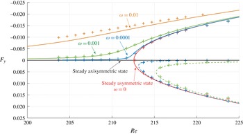
The lift force as a function of the Reynolds number for different rotation rates. The symbols correspond to DNS and the lines correspond to the normal form (6.7) of the imperfect pitchfork bifurcation. The solid lines represent the stable
 $A_{01}$
solution, while the dashed lines represent the unstable
 $A_{02}$
and
 $A_{03}$
solutions.

6.2 Comparison with 3D numerical simulations
We recall that due to the normalization of the direct modes, the lift force is directly given by
 $A$
, allowing one to compare, directly, the solutions of the amplitude equations with the numerical results of figure 4. The comparison is presented in figure 9, which shows that the base flow discussed in § 5.1 is in perfect agreement with the predictions of branch
 $A_{01}$
of the weakly nonlinear model. In addition, the weakly nonlinear approach allows the unveiling of the existence of other disconnected branches of steady solutions for a rotating sphere, corresponding to branches
 $A_{02}$
and
 $A_{03}$
. As shown in figure 9, the global approach also allows the existence of these states to be confirmed, at least for
 $\unicode[STIX]{x1D74E}=0.001$
and
 $\unicode[STIX]{x1D74E}=0.0001$
. On the other hand, for larger values of the rotation rate, these branches become difficult to track. Since they are always unstable, we disregarded these branches in the stability approach described in § 5.2 and concentrated only on the primary branch
 $A_{01}$
.
As expected, the discrepancies between the theory and the DNS data in figure 9 increase with the rotation rate. As the sphere spins faster, the departure from the axisymmetric base flow is greater even for Reynolds numbers far smaller than
 $Re^{SS}$
, and the steady global mode bifurcating from the fixed sphere configuration progressively loses its relevance. It should be noted also that, the weakly nonlinear expansion having been derived in the vicinity of the steady bifurcation, its comparison with DNS data is expected to be less satisfactory as the departure from criticality increases. Figure 9 confirms such behaviour, for all three solution branches and for all rotation rate values.
7 Conclusion
We analysed the stability of a flow past a transversely rotating sphere for various angular velocities (
 $0\leqslant \unicode[STIX]{x1D6FA}\leqslant 1.2$
). The analysis carried out in this work confirms the existence of two different self-sustained modes (modes I and II) in the wake of such rotating spheres. These unsteady modes derive from Hopf supercritical bifurcations. This result was confirmed by using DNS. The first shedding mode is dominated by axially extended streamwise velocity disturbances located past the sphere. The structural sensitivity analysis identifies the wavemaker of these global oscillations in the near-wake region. Mode II presents a frequency that is twice that of mode I but is also characterized by spatial oscillations downstream of the sphere. The core of this instability is in a region of strong shear near the sphere surface. This suggests that this instability could be related to a feedback mechanism involving Kelvin–Helmholtz waves, in accordance with previous experimental and numerical data (Giacobello et al.
Reference Giacobello, Ooi and Balachandar2009).
A weakly nonlinear analysis was derived to investigate the asymmetric wake in the presence of small rotation rates
 $\unicode[STIX]{x1D6FA}$
. We adopted a third-order expansion using a multi-time-scale technique and solved the subsequent hierarchy of equations that was obtained. We showed that this asymmetric state, prior to the vortex shedding, verifies the normal form of an imperfect pitchfork bifurcation whose threshold is the critical
 $Re$
beyond which the non-rotating sphere loses its axisymmetry. Excellent agreement between the theoretical prediction and numerical simulations is reported for all three solution branches. We find one positive branch of solution and two negative ones, as predicted by the matched asymptotic analysis of the normal form. Our results agree well with the well-known Magnus effect predicting the lift produced by a rotating body in a uniform stream.
Appendix A. Stability analysis of the imperfect bifurcation solution branches
The amplitude equation (6.7) can be reduced to the following canonical form:
 $$\begin{eqnarray}\frac{\unicode[STIX]{x2202}X}{\unicode[STIX]{x2202}\bar{t}}=RX-|X|^{2}X+1,\end{eqnarray}$$
where we have introduced the reduced bifurcation parameter
 $$\begin{eqnarray}R=(\unicode[STIX]{x1D706}\unicode[STIX]{x1D74E}^{-2/3}a^{-2/3}\unicode[STIX]{x1D707}^{-2/3})\unicode[STIX]{x1D716}^{2},\end{eqnarray}$$
the reduced amplitude
 $$\begin{eqnarray}X=(\unicode[STIX]{x1D74E}^{-1/3}a^{-1/3}\unicode[STIX]{x1D707}^{1/3})A\end{eqnarray}$$
and the rescaled time scale
 $$\begin{eqnarray}\bar{t}=(\unicode[STIX]{x1D74E}^{-2/3}a^{-2/3}\unicode[STIX]{x1D707}^{1/3})t.\end{eqnarray}$$
Now, we focus our attention on the equilibrium solutions
 $X=X_{0}$
of the amplitude equation. Such solutions correspond to the real roots of the cubic equation
 $$\begin{eqnarray}RX_{0}-|X_{0}|^{2}X_{0}+1=0.\end{eqnarray}$$
Elementary properties of cubic equations (Cardan’s theorem) can be used to show that (A 5) has three branches of solution, and to investigate their behaviour as
 $R$
becomes large:
-
(i) The first one, denoted
$X_{01}$
, exists for all values of
$R$
. Moreover, it displays the following asymptotic behaviours:
$X_{01}\rightarrow -1/R$
as
$R\rightarrow -\infty$
and
$X_{01}\rightarrow \sqrt{R}$
as
$R\rightarrow +\infty$
. -
(ii) The second one, denoted
$X_{02}$
, originates from a saddle point located at
$[R;X]=[3\cdot 2^{-2/3};-2^{-1/3}]$
. It exists only for
$R>3\cdot 2^{-2/3}$
and has the asymptotic behaviour
$X_{02}\rightarrow -1/R$
as
$R\rightarrow +\infty$
. -
(iii) The last one, denoted
$X_{03}$
, originates from the same saddle point, has the same range of existence and has the asymptotic behaviour
$X_{03}\rightarrow -\sqrt{R}$
as
$R\rightarrow +\infty$
.





The asymptotic behaviours presented here as
 $|R|\rightarrow \infty$
provide the ones for
 $\unicode[STIX]{x1D74E}\rightarrow 0$
of the main text, which actually correspond to the distinguished limit
 $\unicode[STIX]{x1D74E}^{2/3}\ll \unicode[STIX]{x1D716}^{2}\ll 1$
.
To investigate the stability of these states, we consider small deviations around each of these equilibrium solutions. We disturb the steady solution of the reduced form so that
 $$\begin{eqnarray}X=(X_{0}+x)\text{e}^{\text{i}\unicode[STIX]{x1D703}}.\end{eqnarray}$$
Injection of this decomposition into (A 1) and linearization in terms of
 $|x|$
and
 $\unicode[STIX]{x1D703}$
lead to
 $$\begin{eqnarray}\displaystyle & \displaystyle \frac{\unicode[STIX]{x2202}x}{\unicode[STIX]{x2202}t}=Rx-3|X_{0}|^{2}\,x, & \displaystyle\end{eqnarray}$$
 $$\begin{eqnarray}\displaystyle & \displaystyle \frac{\unicode[STIX]{x2202}\unicode[STIX]{x1D703}}{\unicode[STIX]{x2202}t}X_{0}=-\unicode[STIX]{x1D703}, & \displaystyle\end{eqnarray}$$
 $$\begin{eqnarray}\unicode[STIX]{x1D70E}_{1}=R-3|X_{0}|^{2}\equiv -1/X_{0}-2|X_{0}|^{2};\quad \unicode[STIX]{x1D70E}_{2}=-{\displaystyle \frac{1}{X_{0}}}.\end{eqnarray}$$
It should be noted that
 $\unicode[STIX]{x1D70E}_{1}$
(respectively
 $\unicode[STIX]{x1D70E}_{2}$
) represents the growth/decay rate of perturbations of the amplitude (respectively the phase).
-
(i) The first branch
$X_{01}$
is always positive, so both eigenvalues are negative. This branch is stable with respect to in-plane and out-of-plane perturbations. -
(ii) The second branch is located in the interval
$-2^{2/3}<X_{02}<0$
. Hence, both eigenvalues are positive: the branch is unstable with respect to both in-plane and out-of-plane perturbations. -
(iii) The third branch verifies
$X_{03}<-2^{2/3}$
. Hence,
$\unicode[STIX]{x1D70E}_{1}$
is negative but
$\unicode[STIX]{x1D70E}_{2}$
is positive. This branch is stable with respect to in-plane perturbations but unstable with respect to out-of-plane perturbations.