


1 Introduction
There are substantial similarities between the class
 $\operatorname {TFAb}$
of torsion-free abelian groups of finite rank and the class
 $\operatorname {FD}$
of fields of characteristic
 $0$
having finite transcendence degree over
 $\mathbb {Q}$
. Both of these well-studied classes consist of countable structures. Except for the trivial group, which we ignore, all are infinite. Hence, we may suppose that the universe of each structure is
 $\omega $
. For each class, there is a dependence notion such that the size of a maximal independent set or basis is well-defined. Each structure is determined, up to isomorphism, by the existential type of a basis. The existential type of the basis says which rational linear combinations are present (in the group), or which polynomials have roots (in the field).
We are particularly interested in the subclasses of
 $\operatorname {TFAb}$
and
 $\operatorname {FD}$
for which the size of a basis is fixed. We write
 $\operatorname {TFAb}_r$
for the class of torsion-free abelian groups of rank r, and
 $\operatorname {FD}_r$
for the class of fields of characteristic
 $0$
and transcendence degree r. Each of these sub-classes has a universal structure. The elements of
 $\operatorname {TFAb}_r$
are precisely the isomorphic copies of the rank r subgroups of the additive group
 $\mathbb {Q}^r$
. The elements of
 $\operatorname {FD}_r$
are precisely the isomorphic copies of degree r subfields of
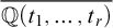 $\overline {\mathbb {Q}(t_1,\ldots ,t_r)}$
, where
 $\mathbb {Q}(t_1,\ldots ,t_r)$
is the purely transcendental extension of
 $\mathbb {Q}$
of degree r, and
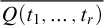 $\overline {Q(t_1,\ldots ,t_r)}$
is its algebraic closure.
The class
 $\operatorname {TFAb}$
and the class
 $\operatorname {FD}$
share many computable-structure-theoretic properties. With one exception, the degree spectra for structures in the two classes are the same—they are the degrees of sets C that are c.e. relative to some fixed d. (See [Reference Frolov, Kalimullin, Miller, Ambos-Spies, Löwe and Merkle7] for
 $\operatorname {FD}$
, and [Reference Coles, Downey and Slaman4] for rank-
 $1$
groups; the proof for all groups in
 $\operatorname {TFAb}$
is analogous.) The lone exception is the trivial group
 $\{0\}$
, which is the unique group in
 $\operatorname {TFAb}_0$
; for fields, in contrast,
 $\operatorname {FD}_0$
contains uncountably many fields, all of which follow the rule above. The proposition below gives the complexities of the isomorphism relations on the subclasses
 $\operatorname {TFAb}_r$
and
 $\operatorname {FD}_r$
. We say only a little about the proof.
Proposition 1.1.
-
(1) For
 $\operatorname {TFAb}_0$
, the isomorphism relation is trivial.
-
(2) For
$\operatorname {FD}_0$
, the isomorphism relation is effective
$\Pi _2$
. -
(3) For
$\operatorname {TFAb}_r$
and
$\operatorname {FD}_r$
, where
$r \ge 1$
, the isomorphism relation is effective
$\Sigma _3$
.


Partial proof.
(2) Fields in
 $\operatorname {FD}_0$
are isomorphic if and only if they satisfy the same existential sentences. This is effective
 $\Pi _2$
.
(3) For
 $\operatorname {TFAb}_r$
and
 $\operatorname {FD}_r$
for
 $r> 0$
, the isomorphism relation is defined by a computable
 $\Sigma _3$
formula saying that there are bases of size r for the two structures such that the existential formulas true of the bases are the same.
The results above are sharp. In [Reference Hirschfeldt, Kramer, Miller and Shlapentokh12, Corollary 2.8], it is shown that the set of pairs of indices for isomorphic computable structures in
 $\operatorname {FD}_0$
is
 $\Pi ^0_2$
. (To see that this is
 $1$
-complete at this level, just notice that when
 $\{ W_e\}_{e\in \omega }$
is the usual effective listing of c.e. sets and
 $p_0<p_1<\cdots $
are the primes,
 $W_i=W_j$
just if
 $\mathbb {Q}(\sqrt {p_n}~:~n\in W_i) \cong \mathbb {Q}(\sqrt {p_n}~:~n\in W_j)$
.) In Section 6, we will show more. The isomorphism relation on
 $\operatorname {FD}_0$
is complete effective
 $\Pi _2$
, and complete
 $\mathbf {\Pi _2}$
, under reducibilities appropriate for the effective Borel, and Borel hierarchies. Similarly, for the classes
 $\operatorname {TFAb}_r$
and
 $\operatorname {FD}_r$
for
 $r> 0$
, we will show that the isomorphism relation is complete effective
 $\Sigma _3$
, and complete
 $\mathbf {\Sigma _3}$
.
In her PhD thesis, Alvir [Reference Alvir1] generalized the notion of finitely generated structure.
Definition 1.2 (Alvir).
A structure
 $\mathcal {A}$
is
 $\alpha $
-finitely generated if there is a finite tuple
 $\bar {a}$
such that for all tuples
 $\bar {b}$
from
 $\mathcal {A}^{<\omega }$
, the orbit of
 $\bar {b}$
over
 $\bar {a}$
is defined by an infinitary
 $\Sigma _\alpha $
formula.
In the classes
 $\operatorname {TFAb}_r$
and
 $\operatorname {FD}_r$
, all structures are
 $1$
-finitely generated, with any basis serving as
 $\bar a$
. The orbit of a tuple
 $\bar b$
over the basis
 $\bar {a}$
is defined by an existential formula. For the groups in
 $\operatorname {TFAb}$
, each element b is actually defined over a basis
 $\bar a$
by a quantifier-free formula of the form
 $n\cdot b = \sum m_ia_i$
with integer coefficients
 $n,m_i$
. In
 $\operatorname {FD}$
, however, existential quantifiers are required, and finitely many distinct tuples
 $\bar b$
can realize the same existential type over
 $\bar a$
. In both classes, viewing the structures as subgroups of
 $\mathbb {Q}^r$
or subfields of
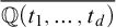 $\overline {\mathbb {Q}(t_1,\ldots ,t_d)}$
endows them (as a class) with computability-theoretic properties different from those they possess as free-standing structures. In particular, the relations of linear independence (for the groups) and algebraic independence (for the fields) are uniformly decidable. In the setting of free-standing structures (which we use), independence is decidable from the atomic diagram of the structure, but not uniformly so, as one needs to know a basis for the structure. (The exceptions are
 $\operatorname {TFAb}_0$
and
 $\operatorname {FD}_0$
, where every basis is empty, and
 $\operatorname {TFAb}_1$
, where every nonzero singleton is a basis).
There are differences among classes
 $\operatorname {TFAb}_r$
for different r that are not accounted for by the complexity of the Scott sentences or the isomorphism relation. There are “invariants” for
 $\operatorname {TFAb}_1$
that are widely accepted as useful. This is not the case for
 $\operatorname {TFAb}_r$
for
 $r> 1$
. Hjorth [Reference Hjorth, Eklof and Göbel13] and Thomas [Reference Thomas27] used the notion of Borel embedding (see Definition 2.1 below) to say in a precise way that the complexity of the invariants increases with r.
Theorem 1.3 (Hjorth, Thomas).
For each
 $r\geq 1$
,
 $\operatorname {TFAb}_r <_B \operatorname {TFAb}_{r+1}$
.
The fact that
 $\operatorname {TFAb}_r \leq _B\operatorname {TFAb}_{r+1}$
simply says that there is a Borel function F that, given the atomic diagram of any
 $G\in \operatorname {TFAb}_{r}$
, produces the atomic diagram of some group
 $F(G)\in \operatorname {TFAb}_{r+1}$
, in such a way that
 $G_0\cong G_1$
if and only if
 $F(G_0)\cong F(G_1)$
. That is, the isomorphism problem for
 $\operatorname {TFAb}_{r}$
is Borel-reducible to that for
 $\operatorname {TFAb}_{r+1}$
. This is not surprising; indeed, a straightforward computable function
 $F(G) = G\times \mathbb {Z}$
can accomplish this task. However, the result of Hjorth and Thomas gives strict Borel reducibility
 $\operatorname {TFAb}_r <_B \operatorname {TFAb}_{r+1}$
, meaning that there is no Borel reduction in the opposite direction:
 $\operatorname {TFAb}_{r+1} \not \leq _B\operatorname {TFAb}_r$
. The proof uses deep results from descriptive set theory. Hjorth and Thomas mentioned the case of fields of finite transcendence degree, but did not address it to any significant extent. Thomas and Velickovic [Reference Thomas and Velickovic28] have shown that the classes
 $\operatorname {FD}_n$
are not strictly increasing under Borel reducibility. There is some (fairly small) n such that for all m,
 $\operatorname {FD}_m\leq _B \operatorname {FD}_n$
.
Our purpose in this article is both to consider the parallel questions for the different ranks
 $\operatorname {FD}_r$
of fields of finite transcendence degree, and to apply the notions of computable reducibility that were subsequently developed in [Reference Calvert, Cummins, Knight and Miller3] and [Reference Miller, Poonen, Schoutens and Shlapentokh22]. For
 $\operatorname {TFAb}$
, the map
 $F(G) = G\oplus \mathbb {Z}$
gives a Turing computable reduction from
 $\operatorname {TFAb}_r$
to
 $\operatorname {TFAb}_{r+1}$
. The result of Hjorth and Thomas says there cannot be a Borel reduction from
 $\operatorname {TFAb}_{r+1}$
to
 $\operatorname {TFAb}_r$
, so there also cannot be a Turing computable reduction. Thus, we have
 $\operatorname {TFAb}_r <_{tc}\operatorname {TFAb}_{r+1}$
. For
 $\operatorname {FD}$
, we will show that for each r, there is a Turing computable reduction from
 $\operatorname {FD}_r$
to
 $\operatorname {FD}_{r+1}$
. (However, this is not nearly so simple as it was for
 $\operatorname {TFAb}$
, as we discuss in Section 5.) We will also give, in Section 4, a Turing computable reduction from each
 $\operatorname {TFAb}_r$
to the corresponding
 $\operatorname {FD}_r$
. All of these reductions will in fact be functorial, a particularly strong type of Turing computable reduction that we describe in Section 2 after giving history and technical details about Borel and Turing computable reductions.
By results of Hjorth [Reference Hjorth, Eklof and Göbel13] and Thomas [Reference Thomas27], there is no Borel reduction from
 $\operatorname {TFAb}_r$
to
 $\operatorname {TFAb}_{r'}$
for
 $r> r'$
. We do not know a specific Borel reduction from
 $\operatorname {FD}_r$
to
 $\operatorname {FD}_{r'}$
for
 $r> r'$
, but results of Thomas and Velickovic imply that for all sufficiently large r, the classes
 $\operatorname {FD}_r$
are
 $\equiv _B$
-equivalent. While the previously mentioned results imply that for large enough d, there is no Borel reduction from
 $\operatorname {FD}_d$
to
 $\operatorname {TFAb}_r$
, we do not yet know a Borel reduction from any
 $\operatorname {FD}_d$
with
 $d> 0$
to any
 $\operatorname {TFAb}_r$
. However, we will show that under countable computable reducibility, all effective
 $\Sigma _3$
equivalence relations on
 $2^\omega $
reduce to
 $\operatorname {TFAb}_r$
. Isomorphism on
 $\operatorname {TFAb}_r$
, for
 $r\geq 1$
, and
 $\operatorname {FD}_r$
are effective
 $\Sigma _3$
. The notion of countable computable reducibility was introduced in [Reference Miller, Cenzer, Porter and Zapletal20].
2 Borel and Turing computable reducibility
For a countable language L,
 $Mod(L)$
is the set of all L-structures with universe
 $\omega $
. For convenience, we may suppose that L consists of relation symbols. We can identify
 $Mod(L)$
with
 $2^\omega $
. Let
 $(\alpha _n)_{n\in \omega }$
be an enumeration of the sentences of form
 $R(\bar {a})$
, where R is a relation symbol of L and
 $\bar {a}$
is an appropriate tuple of natural numbers. We identify the structure
 $\mathcal {A}\in Mod(L)$
with the function
 $f\in 2^\omega $
such that
 $$ \begin{align*}f(n) = \left\{\begin{array}{@{}ll} 1 & \text{if }\mathcal{A}\models\alpha_n\\ 0 & \text{otherwise.} \end{array}\right.\end{align*} $$
We have the usual topology on
 $2^\omega $
, and on
 $Mod(L)$
. The basic clopen sets in
 $Mod(L)$
have the form
 $Mod(\varphi ) = \{ \mathcal {A}\in Mod(L) : \mathcal {A}\models \varphi \} $
, where
 $\varphi $
is finitary and quantifier-free, in the language L with added constants for the natural numbers. The Borel sets are the members of the
 $\sigma $
-algebra generated by the basic clopen sets. The Borel sets may be obtained from the basic clopen sets by closing under countable unions and intersections. The Borel hierarchy classifies Borel sets as
 $\mathbf {\Sigma _\alpha }$
or
 $\mathbf {\Pi _\alpha }$
for countable ordinals
 $\alpha $
. The effective Borel sets are obtained from the basic clopen sets by taking c.e. unions and intersections. The effective Borel hierarchy classifies sets as
 $\Sigma _\alpha $
or
 $\Pi _\alpha $
for computable ordinals
 $\alpha $
. Recall that the
 $L_{\omega _1\omega }$
formulas allow countably infinite disjunctions and conjunctions but only finite strings of quantifiers. The formulas are classified as
 $\Sigma _\alpha $
or
 $\Pi _\alpha $
for countable ordinals
 $\alpha $
. The computable infinitary formulas are formulas of
 $L_{\omega _1\omega }$
in which the disjunctions and conjunctions are over c.e. sets.
Fixing a language L, we consider classes
 $K\subseteq Mod(L)$
such that K is closed under isomorphism; i.e., K is closed under the action of the permutation group
 $S_\infty $
on
 $\omega $
. Lopez-Escobar [Reference Lopez-Escobar19] showed that such a class is Borel if and only if it is axiomatized by a sentence of
 $L_{\omega _1\omega }$
. Vaught [Reference Vaught30] showed that for any countable ordinal
 $\alpha \geq 1$
and any class
 $K\subseteq Mod(L)$
(closed under isomorphism), K is
 $\mathbf {\Sigma _\alpha }$
if and only if it is axiomatized by a
 $\Sigma _\alpha $
sentence of
 $L_{\omega _1\omega }$
. Vanden Boom [Reference Vanden Boom29] proved the effective version of Vaught’s theorem, saying that for any computable ordinal
 $\alpha \geq 1$
, a class
 $K\subseteq Mod(L)$
(closed under isomorphism) is effective
 $\Sigma _\alpha $
if and only if it is axiomatized by a computable
 $\Sigma _\alpha $
sentence.
We have the usual product topology on
 $2^{\omega }\times 2^{\omega }$
, and on
 $Mod(L)\times Mod(L')$
, so we may consider Borel relations on
 $Mod(L)\times Mod(L')$
and Borel functions from
 $Mod(L)$
to
 $Mod(L')$
. Friedman and Stanley [Reference Friedman and Stanley6] introduced the notion of Borel embedding as a precise way to compare the problems of classifying, up to isomorphism, the members of different classes of countable structures.
Definition 2.1 (Friedman–Stanley).
Suppose
 $K\subseteq Mod(L)$
,
 $K'\subseteq Mod(L')$
are closed under isomorphism. A Borel embedding of K in
 $K'$
is a Borel function
 $\Phi :K\rightarrow K'$
such that for all
 $\mathcal {A},\mathcal {B}\in K$
,
 $\mathcal {A}\cong \mathcal {B}$
if and only if
 $\Phi (\mathcal {A})\cong \Phi (\mathcal {B})$
. We say that class K is Borel embeddable in the class
 $K'$
, and we write
 $K \leq _B K'$
, if there is such an embedding.
Friedman and Stanley gave a number of examples involving familiar classes of structures. In particular, they showed that fields and linear orderings lie on top under
 $\leq _B$
. (This means that each of these classes is maximal under
 $\leq _B$
among Borel classes of L-structures for every countable language L.) Using known results, they obtained the fact that
 $2$
-step nilpotent groups lie on top, but showed that abelian p-groups do not. They asked whether the class of torsion-free abelian groups lies on top. After quite some time, Shelah and Paolini [Reference Paolini and Shelah25] gave an affirmative answer. Independently and around the same time, Laskowski and Ulrich [Reference Laskowski and Ulrich17, Reference Laskowski and Ulrich18] provided an alternative proof by showing a more general result that certain classes of countable R-modules lie on top.
Kechris suggested that it would be good to develop an effective version of the notion of Borel embedding. The definition below is from [Reference Calvert, Cummins, Knight and Miller3]. That paper includes results on classes of finite structures, and the structures are allowed to have universe a proper subset of
 $\omega $
. As we said earlier, our structures will have universe
 $\omega $
.
Definition 2.2. Suppose
 $K\subseteq Mod(L), K'\subseteq Mod(L')$
are closed under isomorphism, and
 $L,L'$
are computable languages. Suppose that the classes
 $K,K'$
are both closed under isomorphism. A Turing-computable embedding (or
 $tc$
-embedding) of K in
 $K'$
is a Turing operator
 $\Phi :K\rightarrow K'$
such that
 $\mathcal {A}\cong \mathcal {B}$
if and only if
 $\Phi (\mathcal {A})\cong \Phi (\mathcal {B})$
. If there is such an embedding, we write
 $K\leq _{tc} K'$
. The embedding is called a
 $tc$
-reduction from K to
 $K'$
.
The proof that an operator is one-to-one on isomorphism types often involves showing that the input structure is interpreted (in a uniform way) in the output structure. In [Reference Montalbán24], Montalbán defined a very general notion of effective interpretation, in which the interpreting formulas have no fixed arity. A generalized computable
 $\Sigma _1$
formula is a c.e. disjunction of existential formulas, possibly of different arities. For example, there is a generalized computable
 $\Sigma _1$
formula that defines dependence in
 $\mathbb {Q}$
-vector spaces of tuples of all finite lengths.
Definition 2.3 [Reference Montalbán24, Definition 5.1].
Let
 $\mathcal {A}$
be an L-structure, and let
 $\mathcal {B}$
be an
 $L'$
-structure. For simplicity, we suppose that L is a finite relational language. An effective interpretation of
 $\mathcal {A}$
in
 $\mathcal {B}$
is a tuple of made up of the following: generalized computable
 $\Sigma _1$
formulas defining a set
 $D\subseteq \mathcal {B}^{<\omega }$
, an equivalence relation
 $\sim $
on D, the complementary relation
 $\not \sim $
, and, for each n-ary relation symbol R of L, an n-ary relation
 $R^*$
on D, and the complementary relation
 $\neg (R^*)$
, such that the quotient structure
 $(D,R^*_{R\in L})/_{\!\sim }$
is well-defined and isomorphic to
 $\mathcal {A}$
.
We note that each computable structure
 $\mathcal {A}$
(with universe
 $\omega $
) can be effectively interpreted in every infinite structure
 $\mathcal {B}$
. In the interpretation, the set D is equal to
 $\mathcal {B}^{<\omega }$
, and the element n in
 $\mathcal {A}$
is represented by all n-tuples in
 $\mathcal {B}$
. An effective interpretation of an L-structure
 $\mathcal {A}$
in an
 $L'$
-structure
 $\mathcal {B}$
, as in Definition 2.3 above, gives a uniform effective method of producing a copy of
 $\mathcal {A}$
from any copy of
 $\mathcal {B}$
. In some cases, the same formulas define interpretations in many different structures
 $\mathcal {B}$
. For example, if K is the class of all countable fields (with domain
 $\omega $
), there is an effective interpretation, uniform for every
 $F\in K$
, of the polynomial ring
 $F[X]$
in the field F. (Notice that this cannot be done using the ordinary model-theoretic notion of interpretation, with finitary formulas.) In this way, a uniform effective interpretation may at times produce a Turing-computable embedding of one class K into another class
 $K'$
, as in Definition 2.2. In the example above, the rings
 $E[X]$
and
 $F[X]$
are isomorphic if and only if the fields E and F were isomorphic, and so this is indeed a
 $tc$
-embedding.
Not all Turing-computable embeddings arise from effective interpretations. One example is the Friedman–Stanley embedding of graphs in linear orderings. However, in [Reference Harrison-Trainor, Melnikov, Miller and Montalbán10], Harrison-Trainor, Melnikov, Miller, and Montalbán connected effective interpretations with a notion recently formulated by Miller, Poonen, Schoutens, and Shlapentokh in [Reference Miller, Poonen, Schoutens and Shlapentokh22], which we now describe.
Definition 2.4. For a class K of L-structures, we define the category
 $\text {Iso}(K)$
to have as its objects all structures in K, and to have as its morphisms all isomorphisms between objects in K.
Normally K is closed under isomorphism (the structures all have universe
 $\omega $
). For a single structure
 $\mathcal {A}$
, we define
 $\text {Iso}(\mathcal {A})$
to have
 $ \{ \mathcal {A}'\cong \mathcal {A} : \text {dom}(\mathcal {A}')=\omega \} $
as its objects and all isomorphisms among these objects as the morphisms.
Definition 2.5 [Reference Miller, Poonen, Schoutens and Shlapentokh22, Definition 3.1].
A computable functor from
 $\text {Iso}(K')$
to
 $\text {Iso}(K)$
consists of two Turing functionals
 $\Phi $
and
 $\Psi $
such that:
-
• for every
$\mathcal {B}\in \text {Iso}(K')$
,
$\Phi (\mathcal {B})$
is (the atomic diagram of) a structure in
$\text {Iso}(K)$
, -
• for every isomorphism
$f:\mathcal {B}\to \mathcal {B}'$
in
$\text {Iso}(K')$
,
$\Psi ^{\mathcal {B}\oplus f\oplus \mathcal {B}'}$
is an isomorphism from
$\Phi (\mathcal {B})$
onto
$\Phi (\mathcal {B}')$
, and -
• these two maps define a functor from
$\text {Iso}(K')$
into
$\text {Iso}(K)$
. (Specifically, the map on morphisms respects composition
$\circ $
and preserves the identity isomorphism.)
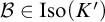


A Turing-computable embedding
 $\Phi $
from
 $K'$
into K is functorial if there exists another functional
 $\Psi $
such that
 $(\Phi ,\Psi )$
is a computable functor from
 $\text {Iso}(K')$
into
 $\text {Iso}(K)$
.
In a functor,
 $\Psi $
ensures that the map
 $\Phi $
on objects preserves the relation of being isomorphic. In an embedding (whether Turing-computable or Borel), one requires
 $\Phi $
also to preserve non-isomorphism, so that
 $\mathcal {B}\cong \mathcal {B}'$
if and only if
 $\Phi (\mathcal {B})\cong \Phi (\mathcal {B}')$
. As an example, the
 $tc$
-embedding described earlier, taking fields F to rings
 $F[X]$
, extends to a computable functor in an obvious way. Harrison-Trainor, Melnikov, Miller, and Montalbán showed that this reflects the uniform effective interpretability of the polynomial rings in the fields. The statement we give here is an amalgam of their Theorems 1.5 and 1.12 from [Reference Harrison-Trainor, Melnikov, Miller and Montalbán10].
Theorem 2.6 [Reference Harrison-Trainor, Melnikov, Miller and Montalbán10].
Let
 $\text {Iso}(\mathcal {A})$
and
 $\text {Iso}(\mathcal {B})$
be categories as above. Then effective interpretations of
 $\mathcal {A}$
in
 $\mathcal {B}$
correspond bijectively to computable functors from
 $\text {Iso}(\mathcal {B})$
into
 $\text {Iso}(\mathcal {A})$
. Each interpretation produces its functor in the natural way, mapping each
 $\widetilde {\mathcal {B}}\cong \mathcal {B}$
to the copy of
 $\mathcal {A}$
given by the interpretation within
 $\widetilde {\mathcal {B}}$
.
More generally, for categories
 $\text {Iso}(K)$
and
 $\text {Iso}(K')$
as above, computable functors from
 $\text {Iso}(K)$
into
 $\text {Iso}(K')$
correspond bijectively to uniform effective interpretations of
 $K'$
in K in the same natural way. (By a uniform effective interpretation, we mean here a set of formulas such that, for every
 $\mathcal {B}\in K$
, the formulas give an effective interpretation in
 $\mathcal {B}$
of some
 $\mathcal {A}\in K'$
.)
In [Reference Harrison-Trainor, Miller and Montalbán11], these results are extended to cover functors and interpretations more broadly. However, for our present investigations, Theorem 2.6 will suffice. Indeed, we will produce some new examples of computable functors, which can then be converted into effective interpretations using the proof of Theorem 2.6 in [Reference Harrison-Trainor, Melnikov, Miller and Montalbán10]. In Section 7, we will consider a different sort of reduction between isomorphism relations on classes of structures, in which only countably many structures from each class are considered at a time. This will give results markedly different from those of Hjorth and Thomas. However, this type of reduction will not be used before Section 7, so we postpone its description until that section.
3 Scott sentences
As mentioned in the introduction, we may describe a structure
 $\mathcal {A}$
in
 $\operatorname {TFAb}$
by giving a basis
 $\bar {a}$
and saying which
 $\mathbb {Q}$
-linear combinations of
 $\bar {a}$
are present. Similarly, we may describe a structure in
 $\operatorname {FD}$
by giving a basis
 $\bar {a}$
and saying which polynomials over
 $\mathbb {Q}(\bar {a})$
have roots. We will see that every structure
 $\mathcal {A}$
in
 $\operatorname {TFAb}_r$
or
 $\operatorname {FD}_r$
has a
 $\Sigma _3$
Scott sentence. We begin with torsion-free abelian groups. We use the standard group language, with one binary operation symbol (for the group operation), one unary operation symbol (for inverse), and one constant symbol (for the identity). Since the identity and inverses are definable without quantifiers, formulas in our language are equivalent to formulas of the same complexity in the language with just the operation symbol.
Proposition 3.1. Every torsion-free abelian group G of finite rank has a
 $\Sigma _3$
Scott sentence, which is G-computable.
Proof. Let G be a subgroup of
 $\mathbb {Q}^n$
of full rank. Consider an n-tuple
 $\bar {a}$
in G that is linearly independent over
 $\mathbb {Z}$
, and let S be the set of
 $\mathbb {Q}$
-linear expressions
 $\lambda (\bar {x})$
such that
 $\lambda (\bar {a})$
is present in G. The Scott sentence says that G is a torsion-free abelian group (
 $\Pi _1$
), and that there is a tuple
 $\bar {x}$
that is independent and such that the
 $\mathbb {Q}$
-linear combinations present are just those in S. To say that
 $\bar {x}$
is independent, we take the conjunction of formulas
 $m_1x_1 + \cdots + m_nx_n\not = 0$
, for integers
 $m_1,\ldots ,m_n$
not all
 $0$
. This is computable
 $\Pi _1$
. To say that
 $y = \lambda (\bar {x})$
for
 $\lambda (\bar {x}) = q_1x_1 + \cdots + q_nx_n$
, where
 $q_i = \frac {m_i}{m}$
, we write
 $my = m_1x_1 + \cdots + m_nx_n$
. This is quantifier-free. To say that the
 $\mathbb {Q}$
-linear combinations present are just those in S, we write
 $\bigwedge _{\lambda \in S}(\exists y) y = \lambda (\bar {x})\ \&\ (\forall y)\bigvee _{\lambda \in S}y = \lambda (\bar {x})$
. This is
 $\Pi _2$
. With a G-oracle we can enumerate S and compute the
 $\Pi _2$
sentence, making the whole Scott sentence G-computable
 $\Sigma _3$
.
Proposition 3.2. There exists
 $G\in \operatorname {TFAb}_1$
with no
 $\Pi _3$
Scott sentence.
Proof. By a result of Montalbán [Reference Montalbán23], there is a
 $\Pi _3$
Scott sentence if and only if the orbits of all tuples are defined by
 $\Sigma _2$
formulas. We describe G with a basis whose orbit is not defined by a
 $\Sigma _2$
formula. Take
 $G\subseteq \mathbb {Q}$
generated by all
 $\frac {1}{p}$
(for all primes p). For a basis, take
 $a = 1$
. This is divisible, just once, by each prime. Suppose
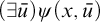 $(\exists \bar {u})\psi (x,\bar {u})$
defines the orbit of
 $1$
in G, where
 $\psi (x,\bar {u})$
is
 $\Pi _1$
, and take
 $\bar {c}$
such that
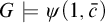 $G\models \psi (1,\bar {c})$
. Each
 $c_i$
has form
 $\frac {m_i}{n_i}$
, where
 $m_i,n_i$
are relatively prime and
 $n_i$
is a product of primes, each occurring at most once. Take a prime q not a factor of any
 $m_i$
or
 $n_i$
. Let
 $a' = \frac {1}{q}$
and let
 $c_i' = \frac {m_i}{qn_i}$
. We have an isomorphism
 $x\rightarrow \frac {x}{q}$
from G onto the extension
 $G'$
generated by
 $\frac {1}{q^2}$
and the elements of G. All formulas true in G of
 $a,\bar {c}$
are true in
 $G'$
of
 $a',\bar {c}'$
. Since
 $G\subseteq G'$
, the
 $\Pi _1$
formulas true in
 $G'$
of
 $a',\bar {c}'$
are also true in G of
 $a',\bar {c}'$
. So, we have
 $G\models (\exists \bar {u})\psi (a',\bar {u})$
. However,
 $a = 1$
is divisible by q in G, while
 $a' = \frac {1}{q}$
is not. So
 $a'$
is not in the orbit of a. Thus, this orbit does not have a
 $\Sigma _2$
definition.
In [Reference Knight, Lange and McCoy14], it is shown that
 $\mathbb {Q}$
is the only rank
 $1$
torsion-free abelian group, up to isomorphism, with a
 $\Pi _2$
Scott sentence.
For fields, we use the usual field language with three binary operation symbols (for addition, subtraction, and multiplication) and two constant symbols (for
 $0$
and
 $1$
). We could omit subtraction and the constants
 $0$
and
 $1$
since these are defined by quantifier-free formulas using just addition and multiplication.
Proposition 3.3. Every field F of characteristic 0 and finite transcendence degree has a
 $\Sigma _3$
Scott sentence, which is F-computable.
The proof of Proposition 3.3 is the same as that for Proposition 3.1, with linear independence replaced by algebraic independence, and taking S to be the set of existential formulas satisfied by the transcendence basis
 $\bar a$
.
We also adapt the proof of Proposition 3.2 to the setting of fields. We use a coding that will appear again in the next section.
Proposition 3.4. There exists
 $F \in \operatorname {FD}_1$
with no
 $\Pi _3$
Scott sentence.
Proof. As in the proof of Proposition 3.2, it suffices to produce
 $F\in \operatorname {FD}_1$
with a basis a whose orbit is not defined by a
 $\Sigma _2$
formula. Let
 $F \subseteq \overline {\mathbb {Q}(t)}$
be the subfield generated by the set of elements
 $t^{1/p}$
, for
 $p>2$
prime, and let
 $a = t$
. (For definiteness: within
 $\overline {\mathbb {Q}(t)}$
, fix a real closed subfield containing t, and choose each
 $t^{1/p}$
to be the unique pth root of t within that subfield.) Suppose
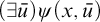 $(\exists \bar {u})\psi (x,\bar {u})$
defines the orbit of t in F, where
 $\psi (x,\bar {u})$
is
 $\Pi _1$
, and take
 $\bar {c}$
such that
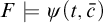 $F\models \psi (t,\bar {c})$
. Each
 $c_i$
is given by an algebraic expression in some finite collection of the generators
 $t^{1/p_{i,j}}$
. Take a prime q different from all of these
 $p_{i,j}$
, and let
 $a' = t^{1/q}$
. Let
 $F'$
be the extension of F by
 $t^{1/q^2}$
. Then there is an isomorphism
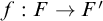 $f:F \to F'$
that fixes
 $\mathbb {Q}\subset F$
and sends t to
 $t^{1/q}$
. Let
 $c_i' = f(c_i)$
. Since f is an isomorphism and
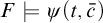 $F\models \psi (t,\bar {c})$
, we have
 $F'\models \psi (t^{1/q},\bar {c'})$
. On the other hand, since
 $F\subseteq F'$
, any
 $\Pi _1$
formulas that are true in
 $F'$
of
 $a',\bar {c}'$
are also true in F of
 $a',\bar {c}'$
. So, we have
 $F\models (\exists \bar {u})\psi (a',\bar {u})$
. However,
 $a = t$
has a qth root in F, while
 $a' = t^{1/q}$
does not. So
 $a'$
is not in the orbit of a. Thus, this orbit does not have a
 $\Sigma _2$
definition.
4 A functorial
$tc$
-embedding of
$\operatorname {TFAb}_r$
into
$\operatorname {FD}_r$


As above, let
 $\operatorname {TFAb}_r$
be the class of torsion-free abelian groups of rank r. We view it as a topological space of structures in the class with domain
 $\omega $
, in the signature with
 $+$
. The topology arises from the identification of atomic diagrams with elements of
 $2^\omega $
, as described in Section 2. Likewise,
 $\operatorname {FD}_r$
is the class of fields of characteristic
 $0$
and of transcendence degree r over the prime subfield
 $\mathbb {Q}$
. As with
 $\operatorname {TFAb}_r$
, we view it as a topological space of structures in the class with domain
 $\omega $
, in the signature with
 $+$
and
 $\cdot $
, as usual for fields. The elements
 $0$
and
 $1$
and the operations of subtraction and division are all definable by quantifier-free formulas, so may be used without hesitation.
 $\operatorname {TFAb}_0$
is trivial. In contrast,
 $\operatorname {FD}_0$
is not trivial: there are many algebraic field extensions of
 $\mathbb {Q}$
, and they have been carefully studied. For rank
 $r\geq 1$
, however,
 $\operatorname {TFAb}_r$
and
 $\operatorname {FD}_r$
show distinct similarities: in both cases the isomorphism relation is effective
 $\Sigma _3$
as stated in Proposition 1.1, and becomes effective
 $\Pi _2$
if one adds r constant symbols to represent the elements of an arbitrary maximal independent set. (Independence refers to linear independence in
 $\operatorname {TFAb}_r$
and to algebraic independence in
 $\operatorname {FD}_r$
.) We also remark that, by [Reference Coles, Downey and Slaman4] and [Reference Frolov, Kalimullin, Miller, Ambos-Spies, Löwe and Merkle7], the Turing degree spectra of groups in
 $\operatorname {TFAb}_r$
(for any fixed
 $r>0$
) are exactly the same as those of fields in
 $\operatorname {FD}_d$
(for any fixed
 $d\geq 0$
): in both cases, they are exactly those sets
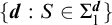 $ \{ \boldsymbol {d} : S\in \Sigma _1^{\boldsymbol {d}} \} $
of Turing degrees defined by the ability to enumerate a specific set
 $S\subseteq \omega $
.
Theorem 4.1. For each finite rank
 $r>0$
, there is a functorial Turing-computable embedding
 $(\Phi ,\Phi _*)$
of
 $\operatorname {TFAb}_r$
into
 $\operatorname {FD}_r$
, uniformly in r.
The image of this functor is not all of
 $\operatorname {FD}_r$
, and we do not claim that it has a computable inverse functor. So, this theorem explains this similarity between the spaces to some extent, but not completely. The rest of this section is dedicated to the proof of Theorem 4.1.
Proof. The input to the operator
 $\Phi $
consists of a rank
 $r>0$
and the atomic diagram (denoted G) of a group from
 $\operatorname {TFAb}_r$
. Now,
 $\Phi $
is required to compute the atomic diagram of a field in
 $\operatorname {FD}_r$
. To avoid confusion, we write
 $\oplus $
for addition in G, and
 $+$
and
 $\cdot $
for the field operations in the output. Given a group G with universe
 $\omega $
,
 $\Phi $
names a corresponding collection of field elements
 $\langle Y_n\rangle _{n\in \omega }$
that we will call monomials. The multiplicative structure of the field on these elements is exactly that given by the group:
 $Y_i\cdot Y_j = Y_k$
if and only if
 $i\oplus j=k$
in G. We therefore view the indices i, j, and k as elements of G. (If
 $e\in G$
is the group identity element, then
 $Y_e$
will be the element
 $1$
; i.e., the multiplicative identity of the field.)
The elements of the field
 $\Phi (G)$
represent quotients
 $$ \begin{align*}\frac{\sum a_n Y_n}{\sum b_nY_n}\end{align*} $$
of finite
 $\mathbb {Q}$
-linear combinations of these monomials (including
 $Y_e=1$
) for which some
 $b_n\neq 0$
. Addition of two
 $\mathbb {Q}$
-linear combinations is done by treating the monomials as indeterminates. Multiplication uses the structure on the monomials:
 $$ \begin{align} \left(\sum a_m Y_m\right)\cdot\left(\sum b_nY_n\right) = \sum_k \left(\sum_{m\oplus n =k} a_mb_n\right)Y_k. \end{align} $$
This makes the
 $\mathbb {Q}$
-linear combinations into a ring R, and Lemma 4.2 below shows it to be an integral domain.
Lemma 4.2. The ring R described above is an integral domain.
Proof. Consider the product in Equation 1. Assume that all coefficients
 $a_m$
and
 $b_n$
are nonzero, and that the factors on the left are both nonzero (so neither sum is empty). Fixing a linearly independent set
 $U=\{ u_1,\ldots ,u_r\}$
in G, we can express each index m and n from G as a
 $\mathbb {Q}$
-linear combination of U: say
 $m=\sum p_{mi}u_i$
and
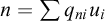 $n=\sum q_{ni}u_i$
. Thus each m corresponds to
 $(p_{m1},\ldots ,p_{mr})\in \mathbb {Q}^r$
, and each n to
 $(q_{n1},\ldots ,q_{nr})\in \mathbb {Q}^r$
. Ordering these r-tuples lexicographically (and comparing individual coefficients under the usual order
 $<$
on
 $\mathbb {Q}$
), fix the particular
 $m_0$
for which
 $(p_{m_01},\ldots ,p_{m_0r})$
is the maximum of the set
 $ \{ (p_{m1},\ldots ,p_{mr}) : a_m\neq 0 \} $
and the
 $n_0$
for which
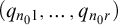 $(q_{n_01},\ldots ,q_{n_0r})$
is the maximum of the set
 $ \{ (q_{n1},\ldots ,q_{nr}) : b_n\neq 0 \} $
. Let
 $k_0=m_0\oplus n_0$
. Then the coefficient of
 $Y_{k_0}$
in the product (on the right side of 1) is simply
 $a_{m_0}b_{n_0}$
: no other pair
 $(m,n)$
of these indices can have
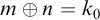 $m\oplus n=k_0$
, because
 $\oplus $
respects the lexicographic order we have chosen. Since
 $a_{m_0}b_{n_0}\neq 0$
, the product on the right is nonzero. This proves the lemma.
We define addition and multiplication on the formal quotients of ring elements
 $\frac {A}{B}$
(for
 $B\not = 0$
) in the obvious way. We also define the obvious congruence relation
 $\sim $
, where
 $\frac {A}{B} \sim \frac {A'}{B'}$
iff
 $AB' = A'B$
. Everything is computable in G. In this way, we obtain the quotient field of the integral domain, whose elements are the
 $\sim $
-equivalence classes of formal quotients
 $\frac {A}{B}$
. We build an isomorphic copy
 $F = \Phi (G)$
with universe
 $\omega $
, and computable in G. More precisely, as each field element is a pair of rational polynomials in
 $Y_n$
, they can be computably identified with
 $\omega $
. And with
 $\sim $
being computable, we may build a computable copy of F by representing each
 $\sim $
-equivalent class by its least member, and addition and multiplication of F are computable in (the multiplication of) G.
To see that the field F has transcendence degree r, let
 $U=\{ u_1,\ldots ,u_r\}$
once again be the fixed linearly independent set in G. Set
 $X_i=Y_{u_i}$
for each
 $i\leq r$
. Now each
 $v\in G$
is a
 $\mathbb {Q}$
-linear combination of the elements of U, say
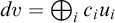 $dv=\bigoplus _{i} c_iu_i$
using integers
 $c_i$
and
 $d\neq 0$
, so the corresponding
 $Y_v^d = Y_{u_1}^{c_1}\cdots Y_{u_r}^{c_r}=\prod X_i^{c_i}$
. Expressing every
 $Y_v$
in this form, we see that the field is generated by rational powers of
 $X_1,\ldots ,X_r$
, and thus has transcendence degree
 $\leq r$
. (This also explains why we refer to the
 $Y_i$
’s as monomials: they are actual monomials in the roots of the basis elements
 $X_i$
.)
We also claim that
 $\{ X_1,\ldots ,X_r\}$
is algebraically independent in F. Suppose some polynomial relation holds on these elements. We may re-express each term in the relation as a single
 $Y_i$
, e.g.,
 $cX_1^2X_2^5 = cY_{u_1}^2Y_{u_2}^5=cY_{2u_1}Y_{5u_2}=cY_{2u_1\oplus 5u_2}$
, so that the entire polynomial equation becomes linear (over
 $\mathbb {Q}$
) in the
 $Y_i$
’s. We have
 $$\begin{align*}0 = \sum c_iY_i ,\end{align*}$$
which implies that every
 $c_i=0$
. However, since U is independent in G, distinct terms
 $X_1^{p_1}\cdots X_r^{p_r}$
yield distinct monomials
 $Y_k$
under this process, with
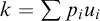 $k=\sum p_iu_i$
. (Otherwise, we would have a nontrivial
 $\mathbb {Q}$
-linear relation on U.) Therefore, there were no repeated terms to combine when the polynomial equation was re-expressed as the
 $\mathbb {Q}$
-linear equation
 $0 = \sum c_iY_i$
, and so the coefficients
 $c_i$
(which must all be zero) are the original coefficients from the polynomial equation on
 $X_1,\ldots ,X_r$
. Thus, these elements are indeed algebraically independent.
It may now be helpful to view
 $X_1,\ldots ,X_r$
as algebraically independent positive real numbers, and to assume that all roots
 $X_i^{\frac 1d}$
used here are positive and real as well. Then the entire field F can be considered as a subfield of the real numbers. It is clear that this construction is functorial, and that the functor is computable. Indeed, if
 $\Phi _*$
is given a group isomorphism
 $g:G_0\to G_1$
, then
 $\Phi _*^{G_0\oplus g\oplus G_1}$
simply maps each
 $Y_n\in F_0=\Phi (G_0)$
to
 $Y_{g(n)}\in F_1=\Phi (G_1)$
, and then extends this map to all
 $\mathbb {Q}$
-linear combinations of the monomials
 $Y_n$
in
 $F_0$
and finally to their quotients. Since the monomials generate
 $F_0$
, this is entirely effective, and it preserves the identity and composition.
Functors must preserve the isomorphism relation on structures, of course, since they map isomorphisms to isomorphisms. However, the theorem also requires the map
 $\Phi $
to preserve non-isomorphism:
 $$ \begin{align*}G_0\cong G_1 \iff \Phi(G_0)\cong\Phi(G_1),\end{align*} $$
so that
 $\Phi $
will be a Turing-computable embedding of
 $\operatorname {TFAb}_r$
into
 $\operatorname {FD}_r$
as well as being functorial.
So, it remains to show that when
 $G\not \cong \widetilde {G}$
, we must get non-isomorphic fields
 $F=\Phi (G)$
and
 $\widetilde {F}=\Phi (\widetilde {G})$
as outputs. From here on, let
 $f:F \to \widetilde {F}$
be a field isomorphism. We need to show
 $G\cong \widetilde {G}$
. We continue to use the transcendence basis
 $X_1,\ldots ,X_r$
of F built from a basis U for G, and the transcendence basis
 $\tilde {X}_1,\ldots ,\tilde {X}_r$
for
 $\widetilde {F}$
built in the analogous manner from some basis of
 $\widetilde {G}$
. The basis U of G naturally induces an embedding from G to
 $\mathbb {Q}^r$
, so we consider G as a subgroup of
 $\mathbb {Q}^r$
from now on (and similarly for
 $\widetilde {G}$
).
Noting that monomials in F correspond to elements in G, if f sends monomials in F to monomials in
 $\widetilde {F}$
and vice versa, then it will induce a map from G to
 $\widetilde {G}$
, which can be shown to be a bijection. However, not every isomorphism
 $f: F\to \widetilde {F}$
sends monomials to monomials. For example, when
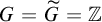 $G = \widetilde {G}= \mathbb {Z}$
, we have
 $F = \widetilde {F} = \mathbb {Q}(X)$
and the map
 $f: F \to \widetilde {F}$
with
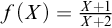 $f(X) = \frac {X+1}{X+2}$
is an isomorphism that maps the monomial X to some non-monomial. While it is still true that
 $F\cong \widetilde {F}$
implies
 $G\cong \widetilde {G}$
(both in this case and in general), the proof is more delicate and requires us to consider the set of monomials that are sent to monomials by f.
Definition 4.3.
-
(1) Let
$m:G\to F$
be the function that sends an element in G to its associated monomial in F; i.e.,
$m(a_1,\ldots , a_r) =X_1^{a_1}\cdots X_r^{a_r} $
. -
(2) Let
$H \subseteq G$
be the set of group elements such that the corresponding monomial in F is sent by f to a monomial; i.e.,
$$ \begin{align*}H = \{g\in G \mid f(m(g))\text{ is a monomial of }\widetilde{F}\}.\end{align*} $$




Similarly define
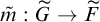 $\tilde m:\widetilde {G} \to \widetilde {F}$
and
 $\widetilde {H}\subseteq \widetilde {G}$
.
Recall that a subgroup H of an additive group G is said to be pure if for every
 $g\in G$
and
 $k\in \mathbb {Z}$
, if
 $kg$
is in H, then g is in H.
Proposition 4.4. For the groups
 $H\subseteq G$
and
 $\widetilde {H}\subseteq \widetilde {G}$
in Definition 4.3, H is a pure subgroup of G, and
 $\widetilde {H}$
is a pure subgroup of
 $\widetilde {G}$
. Furthermore, f maps
 $m(H)$
onto
 $\tilde m(\widetilde {H})$
. The restriction of f taking
 $m(H)$
onto
 $\tilde m(\widetilde {H})$
, is a bijection that respects field multiplication. Hence, f maps H isomorphically onto
 $\widetilde {H}$
.
Proof. Suppose
 $g\in G$
and
 $kg\in H$
for some
 $k \in \mathbb {N}$
. Then
 $m(g)^k = m(kg)$
, so
 $f(m(g))^k = f(m(kg))$
is a monomial. However, if
 $f(m(g))$
were not a monomial, then
 $f(m(g))^k$
would also not be a monomial. Thus,
 $f(m(g))$
must be a monomial, and
 $g\in H$
. Hence, H is a pure subgroup of G. Similarly,
 $\widetilde {H}$
is a pure subgroup of
 $\widetilde {G}$
. By definition, every element of
 $m(H) \subseteq m(G)$
is a monomial. Thus, for every
 $h\in H$
,
 $f(m(h))$
and
 $f^{-1}(f(m(h))) = m(h)$
are both monomials, so
 $f(m(h))$
is in
 $\tilde m(\widetilde {H})$
. Then f maps
 $m(H)$
to
 $\tilde m(\widetilde {H})$
in a well-defined way. Since f is injective and respects multiplication, the restriction that takes
 $m(H)$
to
 $\tilde m(\widetilde {H})$
is also injective and respects multiplication. For
 $a \in \tilde m(\widetilde {H})$
,
 $f^{-1}(a)$
is a monomial, and
 ${f(f^{-1}(a)) = a}$
is also a monomial. Thus,
 $f^{-1}(a) \in m(H)$
. This shows that f maps
 $m(H)$
onto
 $\tilde m(\widetilde {H})$
.
The previous proposition shows that the monomials that are sent to monomials by f indeed induce an isomorphism on the corresponding subgroup H and
 $\widetilde {H}$
. However, as we have seen previously, not all monomials need to be sent to monomials. Instead, we will show the previous example with
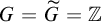 $G = \widetilde {G} = \mathbb {Z}$
is essentially the “only” example where a monomial can be sent to a non-monomial. Namely, we will show that
 $G\cong H\oplus \mathbb {Z}^k$
and
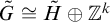 $\tilde G\cong \tilde H\oplus \mathbb {Z}^k$
, for
 $k = r - j$
where j is the rank of H and
 $\widetilde {H}$
. This will establish that
 $G \cong \widetilde {G}$
. We will need a lemma by Schinzel.
Lemma 4.5 [Reference Schinzel26, Lemma 1].
Let K be a field of characteristic 0. If
 $g\in K[x] \setminus \{0\}$
has in the algebraic closure of K a nonzero root of multiplicity at least m, then the polynomial g has at least
 $m+1$
terms (with nonzero coefficients).
As a warm-up example, letting
 $G =\mathbb {Q}$
, we will show that f must send monomials to monomials. Let
 $X\in F$
be the element corresponding to
 $1\in \mathbb {Q}$
. Since G has rank 1, F and
 $\widetilde {F}$
have transcendence degree 1, so
 $\widetilde {G}$
also has rank 1. Let
 $\tilde X$
be a monomial of
 $\widetilde {F}$
, so every other monomial of
 $\widetilde {F}$
is a rational power of
 $\tilde X$
. Suppose
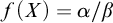 $f(X) = \alpha /\beta $
is reduced and such that
 $\alpha $
and
 $\beta $
are polynomials in some
 $\tilde X^t$
with
 $t\in \mathbb {Q}$
, and
 $\alpha $
and
 $\beta $
are not both monomials. Let T be the sum of the numbers of terms in
 $\alpha $
and
 $\beta $
. Then
 $1/T \in \mathbb {Q}$
so
 $X^{1/T}\in F$
. Suppose
 $m(X^{1/T}) = \alpha '\beta '$
is reduced. We have
 $m(X) = m(X^{1/T})^T$
, so
 $\alpha ^{\prime T} = \alpha $
. If
 $\alpha '$
is a monomial, then
 $\alpha = \alpha ^{\prime T}$
must also be a monomial, a contradiction. However, if
 $\alpha '$
is not a monomial, then it must have a non-zero root. So
 $\alpha = \alpha ^{\prime T}$
must have a nonzero root of multiplicity at least T, and by the previous lemma, must have at least
 $T+1$
terms, also a contradiction. So
 $m(X)$
must be a monomial, and since the other monomials in F are all rational powers of X, they are also sent to monomials.
We generalize this argument to higher rank to obtain the following key technical lemma, which in shows that G must be a direct sum of H and some
 $\mathbb {Z}^k$
(Lemma 4.7). In particular, the above argument is used in Step 0.5 and Step 1.5 to achieve condition (3). Item (2) is a technical condition that we need to maintain in order to apply Lemma 4.5.
We will use the following notation. For an element
 $g\in G$
, let
 $|g|$
be the usual r-dimensional Euclidean norm of
 $g\in \mathbb {Q}^r$
, and endow G with the topology induced by the Euclidean distance. Let
 $\bar H$
be the
 $\mathbb {Q}$
-span of H in
 $\mathbb {Q}^r$
. Since H is a pure subgroup of G, we have that
 $\bar H\cap G = H$
. Let
 $\pi :\mathbb {Q}^r \to \mathbb {Q}^r/\bar H$
be the natural quotient map.
Lemma 4.6. There is some
 $\epsilon> 0$
such that for every nonzero
 $g\in G\setminus H$
,
 $|g|> \epsilon $
.
Proof. If
 $G = H$
, then the statement is vacuously true. Thus, we assume that
 $G \neq H$
. Toward a contradiction, assume that for every
 $\epsilon> 0$
there is some nonzero
 $g\in G\setminus H$
such that
 $|g| < \epsilon $
. We claim that there are some
 $k\in \mathbb {N}$
and a sequence of elements
 $g_1, g_2, \ldots , g_k\in G\setminus H$
such that:
-
(1)
$\pi (g_1), \ldots , \pi (g_{k-1})$
is linearly independent and
$\pi (g_k)$
is a
$\mathbb {Q}$
-linear combination of them. -
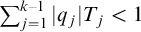
(2) Let
$\pi (g_k) = \sum _{j=1}^{k-1} q_j\pi (g_j)$
. For every
$1 \le i \le k$
, let
$f(m(g_i)) = \alpha _i/\beta _i$
and
$T_i$
be the sum of the numbers of terms in
$\alpha _i$
and
$\beta _i$
. Then
$\sum _{j=1}^{k-1}|q_j|T_j < 1$
. -
(3) For each
$1\le i\le k$
,
$g_i$
is not divisible by any
$n> 1$
in G. Namely, for each
$n> 1$
, there exists no x with
$n x = g_i$
.










We construct the sequence by the following process.
Step 0: Pick any
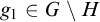 $g_1\in G\setminus H$
.
Step 0.5: We claim that there is a largest
 $n\ge 1$
so that
 $g_1$
is divisible by n, so that we can replace
 $g_1$
by
 $\frac 1n g_1$
to achieve (3). Since
 $g_1$
is not in H, we know
 $f(m(g_1))$
is not a monomial. Thus, we write
 $f(m(g_1)) = \alpha _1/\beta _1$
and let
 $T_1$
be the sum of the numbers of terms in
 $\alpha _1$
and
 $\beta _1$
. Suppose there is some g and
 $n> 1$
with
 $g_1 = ng$
. Since H is a subgroup and
 $g_1 = ng\notin H$
, we also have
 $g\notin H$
. We claim that then
 $n < T_1$
. Let
 $f(m(g)) = \alpha /\beta $
, so
 $\alpha _1/\beta _1 = (\alpha /\beta )^n$
. By replacing each
 $\tilde X_1, \ldots , \tilde X_r$
by
 $X^{t_1}, \ldots , X^{t_r}$
with
 $1 \ll t_1 \ll \cdots \ll t_r \in \mathbb {N}$
, we may assume
 $\alpha (X^{t_1},\ldots , X^{t_r})$
,
 $\alpha _1(X^{t_1},\ldots , X^{t_r})$
,
 $\beta (X^{t_1},\ldots ,X^{t_r})$
,
 $\beta _1(X^{t_1},\ldots ,X^{t_r})$
have the same number of terms as
 $\alpha , \alpha _1, \beta , \beta _1$
, respectively, and
 $\alpha (X^{t_1},\ldots , X^{t_r})$
does not divide
 $\beta (X^{t_1},\ldots ,X^{t_r})$
. Since
 $g \notin H$
, without loss of generality, assume
 $\alpha $
is not a monomial and choose a root
 $\xi $
of
 $\alpha (X^{t_1},\ldots , X^{t_r})$
that is not a root of
 $\beta (X^{t_1},\ldots , X^{t_r})$
. Then
 $\xi $
is a root of
 $\alpha _1(X^{t_1},\ldots , X^{t_r})$
of multiplicity at least n. Thus, by Lemma 4.5,
 $\alpha _1$
has at least
 $n+1$
terms, which establishes
 $n+1 < T_1$
. Hence there must be a largest n that divides
 $g_1$
.
Step 1: If the current tuple
 $\pi (g_1), \pi (g_2), \dots , \pi (g_{i-1})$
is linearly independent, we proceed to find
 $g_i$
. Define
 $\alpha _j, \beta _j, T_j$
as in (2) and
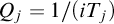 $Q_j = 1/(iT_j)$
. Let S be the pure subgroup of
 $G/H$
generated by
 $\pi (g_1),\ldots , \pi (g_{i-1})$
and let
 $S_0 = \{\sum q_j\pi (g_j) : (\forall j) |q_j| < Q_j\}$
. Then
 $S_0$
is an open set in S, so its preimage
 $\pi ^{-1}(S_0)$
is also an open set in
 $\pi ^{-1}(S)$
. Thus, there is some
 $\epsilon _i$
such that the ball B of radius
 $\epsilon _i$
around the origin satisfies
 $B \cap \pi ^{-1}(S)\subset \pi ^{-1}(S_0)$
. By assumption, there is some
 $g_i \in G \setminus H$
with
 $|g_i| < \epsilon _i$
. Use this as our next
 $g_i$
.
Step 1.5: If
 $g_i$
is divisible by some
 $n> 1$
, repeat the argument in Step 0.5: let
 $n>1$
be the largest number dividing
 $g_i$
, and replace
 $g_i$
by
 $\frac 1n g_i$
.
Step 2: If the current tuple
 $\pi (g_1), \pi (g_2), \dots , \pi (g_i)$
is linearly independent, return to Step 1 and find the next
 $g_{i+1}$
. If
 $\pi (g_1), \pi (g_2), \dots , \pi (g_i)$
is linearly dependent, then set
 $k = i$
and return the tuple. As the range of
 $\pi $
is a quotient of
 $\mathbb {Q}^r$
, it is finite-dimensional. Thus
 $\pi (g_1), \pi (g_2), \dots , \pi (g_i)$
must eventually be linearly dependent, for some i, so the process will halt.
Note that the Step 1 and 2 loop guarantees (1), and Step 0.5 and 1.5 guarantee (3). Thus, we only need to check that the constructed sequence satisfies (2). As
 $\pi (g_1), \cdots , \pi (g_{k-1})$
is linearly independent and
 $\pi (g_1), \ldots , \pi (g_{k})$
is linearly dependent, there is a unique way to write
 $\pi (g_k) = \sum _{j=1}^{k-1} q_j\pi (g_j)$
. By the choice in Step 1 (and the fact that Step 1.5 will only decrease the norm of
 $g_k$
so will not affect the containment), we have
 $g_k \in B \cap \pi ^{-1}(S)\subset \pi ^{-1}(S_0)$
, so
 $\pi (g_k) \in S_0$
. This means that
 $\pi (g_k)$
can be written as a linear combination of
 $\pi (g_j)$
where the jth coefficient is less than
 $Q_j$
. However, such a linear combination is unique, so we must have
 $|q_j| < Q_j$
for every j (by the choice of
 $S_0$
) and
 $\sum _{j=1}^{k-1}|q_j|T_j < \sum _{j=1}^{k-1}Q_jT_j < \sum _{j=1}^{k-1}1/k < 1$
.
Now, we have a sequence of nonzero
 $g_1, g_2, \ldots , g_k\in G\setminus H$
satisfying (1) to (3). By clearing denominators in the
 $q_i$
, we can find some
 $n_i\in \mathbb {Z}$
such that
 $n_k \neq 0$
and
 $\sum n_i\pi (g_i) = 0$
. By replacing
 $g_i$
with
 $-g_i$
if necessary, we will assume each
 $n_i \ge 0$
for simplicity. From (2), we have
 $\sum _{i=1}^{k-1}(n_i/n_k)T_j < 1$
.
Define
 $h = \sum n_ig_i$
. We have
 $\pi (h) = 0$
, so
 $h \in \bar H$
, but also
 $h \in G$
, so we have
 $h\in H$
. Thus,
 $f(m(h))$
is a monomial. Now working in the field, we have
 $$ \begin{align*}m(h) = m(\sum n_ig_i) = \prod m(n_ig_i) = \prod(m(g_i))^{n_i}.\end{align*} $$
Applying f, we then have
 $$ \begin{align*}f(m(h)) = \prod (\alpha_i/\beta_i)^{n_i}.\end{align*} $$
Recall that
 $\alpha _i$
and
 $\beta _i$
are quotients of polynomials in
 $\tilde X_1, \ldots , \tilde X_r$
, potentially with rational exponents. Take
 $1 \ll t_1 \ll \cdots \ll t_r \in \mathbb {N}$
such that
 $t_i$
is a common multiple of all the denominators of powers of
 $\tilde X_i$
in
 $\alpha _i$
and
 $\beta _i$
. Consider
 $\alpha _i(X^{t_1},\ldots , X^{t_r})$
and
 $\beta _i(X^{t_1},\ldots ,X^{t_r})$
. Since
 $1 \ll t_1 \ll \cdots \ll t_r \in \mathbb {N}$
, we have that
 $\alpha _i(X^{t_1},\ldots , X^{t_r})$
and
 $\beta _i(X^{t_1},\ldots ,X^{t_r})$
have the same number of terms as
 $\alpha _i$
and
 $\beta _i$
, respectively. Furthermore, since
 $t_i$
is a common multiple of all denominators of powers of
 $\tilde X_i$
in
 $\alpha _i$
and
 $\beta _i$
, we have that
 $\alpha _i(X^{t_1},\ldots , X^{t_r})$
and
 $\beta _i(X^{t_1},\ldots ,X^{t_r})$
have integral exponents, thus are in
 $\mathbb {Q}[X]$
. For notational simplicity, we will from now on write
 $\alpha _i = \alpha _i(X^{t_1},\ldots , X^{t_r}) \in \mathbb {Q}[X]$
, etc.
Since
 $\alpha _k/\beta _k \neq 1 $
and they are not both monomials, by taking the reciprocal if necessary, there must be some root
 $0 \neq \xi \in \mathbb {C}$
of
 $\alpha _k$
that is not a root of
 $\beta _k$
. We give a lower bound on the multiplicity of
 $\xi $
as a root of
 $\prod (\alpha _i/\beta _i)^{n_i}$
. First,
 $\xi $
is a root of
 $\alpha _k$
and not a root of
 $\beta _k$
, so
 $(\alpha _k/\beta _k)^{n_k}$
contributes at least
 $n_k$
to the multiplicity of
 $\xi $
(as a root of
 $\prod (\alpha _i/\beta _i)^{n_i}$
). We then consider
 $(\alpha _i/\beta _i)^{n_i}$
for
 $i < k$
, which could potentially contribute negatively to the multiplicity of
 $\xi $
(as a root of
 $\prod (\alpha _i/\beta _i)^{n_i}$
) if
 $\xi $
is a root of
 $\beta _i$
. However, since each
 $\beta _i$
has at most
 $T_i$
terms, by Lemma 4.5, if
 $\xi $
is a root of
 $\beta _i$
, its multiplicity is at most
 $T_i$
. Thus, the contribution of each
 $(\alpha _i/\beta _i)^{n_i}$
to the multiplicity of
 $\xi $
(as a root of
 $\prod (\alpha _i/\beta _i)^{n_i}$
) is at least
 $-n_iT_i$
.
Thus, as a root of
 $\prod (\alpha _i/\beta _i)^{n_i}$
,
 $\xi $
has multiplicity at least
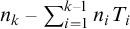 $n_k-\sum _{i = 1}^{k-1} n_iT_i$
. Note that
 $n_k-\sum _{i = 1}^{k-1} n_iT_i = n_k(1-\sum _{i = 1}^{k-1} (n_i/n_k)T_i)> 0$
by condition (2). Thus,
 $\xi $
is a root of
 $f(m(h)) = \prod (\alpha _i/\beta _i)^{q_i}$
. However,
 $f(m(h)) = f(m(h))(X^{t_1},\ldots , X^{t_r})$
is a monomial and has no nonzero root, a contradiction. Thus, the lemma follows.
Lemma 4.7. Suppose there is some
 $\epsilon>0$
such that for every nonzero
 $g\in G\setminus H$
,
 $|g|> \epsilon $
. Then
 $G = H\oplus \mathbb {Z}^k$
for some
 $k\in \mathbb {N}$
.
Proof. We first work in
 $\mathbb {Q}^r/\bar H$
. Since there is a ball that intersects
 $G\setminus H$
trivially, the image
 $\pi (G)$
is discrete. Thus,
 $\pi (G)$
is isomorphic to
 $\mathbb {Z}^k$
for some k. Let
 $g_1, \ldots , g_k \in G$
such that
 $\pi (g_1), \ldots , \pi (g_k)$
is a free generating set of
 $\pi (G)$
. Note that
 $g_i$
are linearly independent.
We now show that
 $G = H \oplus \langle g_1\rangle \oplus \cdots \oplus \langle g_k\rangle $
. Let
 $g \in G$
. Then
 $\pi (g) = \sum q_i\pi (g_i)$
for some
 $q_i\in \mathbb {N}$
. Then
 $g-\sum q_ig_i$
is in
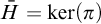 $\bar H = \ker (\pi )$
and is also in G, so
 $g-\sum q_ig_i\in H$
. Thus
 $g \in H+ \langle g_1\rangle +\cdots +\langle g_k\rangle $
. Now, suppose for some
 $h,h' \in H$
and
 $q_i,q_i' \in \mathbb {Z}$
, we have
 $h+\sum q_ig_i = h'+\sum q_i' g_i$
. Considering
 $\pi (G)$
and recalling that the elements
 $\pi (g_i)$
form a free generating set, we must have
 $q_i = q_i'$
. Thus, by canceling, we also have
 $h = h'$
, so the sum
 $H+ \langle g_1\rangle +\cdots +\langle g_k\rangle $
is direct. Thus,
 $G = H \oplus \langle g_1\rangle \oplus \cdots \oplus \langle g_k\rangle \cong H \oplus \mathbb {Z}^k$
.
Combining Lemmas 4.6 and 4.7, we see that
 $G= H\oplus \mathbb {Z}^k$
. On the other hand,
 $\widetilde {G}$
satisfies exactly the same conditions with
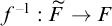 $f^{-1}:\widetilde {F} \to F$
a field isomorphism, so
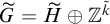 $\widetilde {G} = \widetilde {H}\oplus \mathbb {Z}^{\tilde {k}}$
. Since H and
 $\widetilde {H}$
are pure groups, we have
 $\operatorname {rank}(G) = \operatorname {rank}(H)+k$
and
 $\operatorname {rank}(\widetilde {G}) = \operatorname {rank}(\widetilde {H})+\tilde k$
. We also have
 $H \cong \widetilde {H}$
by Proposition 4.4, so
 $k = \tilde k$
. Finally, we have that if
 $F\cong \widetilde {F}$
, then
 $G= H\oplus \mathbb {Z}^k \cong \widetilde {H}\oplus \mathbb {Z}^{\tilde k}= \widetilde {G}$
. This completes the proof of Theorem 4.1.
In the proof, we need to fix an embedding of G into
 $\mathbb {Q}^r$
(the paragraph before Definition 4.3). However, this requires having a basis for G, which cannot in general be found computably. Furthermore, we also need to find a generating set of
 $\pi (G) \cong \mathbb {Z}^k$
in Lemma 4.7, which also may not be computable. The following question remains open.
Question 4.8. If
 $G, H\in \operatorname {TFAb}_r$
and
 $g: \Phi (G) \to \Phi (H)$
is an isomorphism, then
 $G\cong H$
by Theorem 4.1, and by relative computable categoricity there must exist a
 $(G\oplus H)$
-computable isomorphism
 $f:G \to H$
. Can we compute such an isomorphism uniformly from G, H, and g?
(We note that, although relative computable categoricity for groups in
 $\operatorname {TFAb}_r$
may not have been stated in the literature as yet, it is readily seen. One adds r constants to the language and uses them to represent elements of a basis of one copy G and the isomorphic images of those elements in H. Then every element of G is quantifier-free definable in the expanded signature, enabling one to determine its image in H. The same argument fails for
 $\operatorname {FD}_r$
, where, even with a fixed basis, orbits under automorphisms may be finite sets instead of merely singletons.)
5
$\operatorname {FD}_r$
into
$\operatorname {FD}_{r+1}$


In this section, we show that for every
 $r \ge 0$
, we have
 $\operatorname {FD}_r \le _{tc}\operatorname {FD}_{r+1}$
via a computable functor. For
 $\operatorname {TFAb}$
, if
 $A,B \in \operatorname {TFAb}_r$
, then
 $A \cong B$
if and only if
 $A\oplus \mathbb {Z} \cong B \oplus \mathbb {Z}$
. Thus,
 $\Phi (A) = A\oplus \mathbb {Z}$
gives a Turing computable embedding witnessing
 $\operatorname {TFAb}_r \le _{tc} \operatorname {TFAb}_{r+1}$
. However, for
 $\operatorname {FD}$
, there are two fields
 $E \not \cong F\in \operatorname {FD}_r$
such that
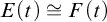 $E(t) \cong F(t)$
(see [Reference Beauville, Colliot-Thélène, Sansuc and Swinnerton-Dyer2]). We will use the henselization of a field to define a Turing computable embedding.
We first consider the case when
 $r= 0$
. In this case, the purely transcendental extension suffices.
Proposition 5.1.
 $\operatorname {FD}_0\leq _{tc} \operatorname {FD}_{1}$
. Furthermore, the Turing computable embedding is functorial (i.e., it can be extended to a computable functor).
Proof of Proposition 5.1.
Consider a Turing operator
 $\Phi $
that takes
 $A\in \operatorname {FD}_0$
to a purely transcendental extension
 $A(t)$
. For this, we need to know when one rational function
 $f(t)$
(with coefficients in A) is equal to another
 $g(t)$
. It is enough to know when one polynomial
 $p(t)$
is equal to another
 $q(t)$
. This happens just when the difference is equal to
 $0$
. In the purely transcendental extension, this happens exactly when each coefficient is 0.
To complete the proof of Proposition 5.1, we need the following lemma.
Lemma 5.2. For
 $A,A'\in \operatorname {FD}_0 $
, if f is an isomorphism from
 $A(t)$
onto
 $A'(t')$
, then
 $A \cong A'$
via
 $f|_A$
.
Proof of Lemma 5.2.
Let
 $f(t) = x$
, and let
 $f(A) = B$
. Since
 $A(t)$
is a purely transcendental extension of A,
 $B(x)$
is a purely transcendental extension of B, and the image
 $B(x)$
of f must equal
 $A'(t')$
. Then
 $A'$
and B are algebraic over
 $\mathbb {Q}$
. Now, Luroth’s theorem says that
 $A'$
is relatively algebraically closed in
 $A'(t)$
. That is, if
 $c\in A'(t)$
is algebraic over
 $\mathbb {Q}$
, then it is already present in
 $A'$
. Thus,
 $B\subseteq A'$
. Similarly, B is relatively algebraically closed in
 $B(x)$
; if
 $c\in B(x)$
is algebraic over
 $\mathbb {Q}$
, then it is already present in B. Therefore,
 $A'\subseteq B$
. So, f maps A isomorphically onto
 $A'$
.
Conversely, it is clear that if
 $A\cong A'$
, then
 $A(t)\cong A'(t')$
. Moreover, whenever
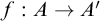 $f:A\to A'$
is an isomorphism, we can extend f to an isomorphism
 $\overline {f}:A(t)\to A'(t')$
by defining
 $f(t)=t'$
. Since
 $A(t)$
is constructed so that its subset A of constant rational functions is uniformly decidable within
 $A(t)$
, this
 $\overline {f}$
is computable uniformly from f, A, and
 $A'$
. The choice of
 $\overline {f}$
respects composition and preserves the identity, so we have a computable functor from
 $\operatorname {FD}_0$
to
 $\operatorname {FD}_1$
.
Similar to the results of Hjorth and Thomas on
 $\operatorname {TFAb}_r$
, this embedding is strict.
Proposition 5.3.
 $\operatorname {FD}_1\not \leq _{tc} \operatorname {FD}_0$
.
Proof. Existential sentences, saying which polynomials over
 $\mathbb {Q}$
have roots, are enough to distinguish non-isomorphic elements of
 $\operatorname {FD}_0$
. We will use the Pullback theorem [Reference Knight, Miller and Vanden Boom15]. First, we show that there are non-isomorphic elements of
 $\operatorname {FD}_1$
with the same existential theory. For this, consider a chain of three fields. The first,
 $A_0$
, is the algebraic closure of
 $\mathbb {Q}$
. The second,
 $A_1$
, is
 $A_0(t)$
, a purely transcendental extension of
 $A_0$
. The third,
 $A_2$
, is the algebraic closure of
 $A_1$
. Now,
 $A_0$
and
 $A_2$
satisfy the same theory—that of algebraically closed fields of characteristic
 $0$
. Existential sentences are preserved under extension, so those true in
 $A_0$
are true in
 $A_1$
and those true in
 $A_1$
are true in
 $A_2$
, matching those true in
 $A_0$
. Then
 $A_1$
and
 $A_2$
are non-isomorphic elements of
 $\operatorname {FD}_1$
with the same existential theory. If
 $\Phi $
were a
 $tc$
-reduction to
 $\operatorname {FD}_0$
, we would have
 $\Phi (A_1)\not \cong \Phi (A_2)$
, so there would be an existential sentence
 $\varphi $
true in just one of the two. The pullback
 $\varphi ^*$
is a computable
 $\Sigma _1$
sentence true in just one of
 $A_1$
and
 $A_2$
. Now,
 $\varphi ^*$
is a disjunction of existential sentences, one of which is true in just one of
 $A_1,A_2$
. This is a contradiction.
We can extend the previous result to Borel embeddings.
Proposition 5.4.
 $\operatorname {FD}_1\not \leq _B \operatorname {FD}_0$
.
Proof. Suppose
 $\Phi $
is a Borel embedding of
 $\operatorname {FD}_1$
in
 $\operatorname {FD}_0$
.
Claim 1: There is a Borel reduction of isomorphism on
 $\operatorname {FD}_0$
to
 $=$
(equality on sets). (In fact, the output set is
 $\Sigma ^0_1$
uniformly relative to the input field.)
Proof of Claim 1.
Let
 $(p_n)_{n\in \omega }$
be a computable list of the polynomials
 $p(x)$
with coefficients in
 $\mathbb {Z}$
. Let
 $\Psi $
take the field
 $\mathcal {A}\in \operatorname {FD}_0$
to the set
 ${S = \{n:\mathcal {A}\models (\exists x)p_n(x)= 0\}}$
. We have
 $\mathcal {A}\cong \mathcal {A}'$
if and only if
 $\Psi (\mathcal {A}) = \Psi (\mathcal {A}')$
.
Recall that
 $E_0$
(Vitali equivalence) is the equivalence relation on
 $2^\omega $
such that
 $fE_0 g$
just if f and g differ finitely; i.e., for all sufficiently large n,
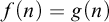 $f(n) = g(n)$
.
Claim 2: There is a Borel reduction, even a
 $tc$
-reduction, of
 $E_0$
to isomorphism on
 $\operatorname {TFAb}_1$
.
Proof of Claim 2.
Let
 $(p_n)_{n\in \omega }$
be a computable enumeration of the primes. Let
 $\Psi '$
take f to a computable copy of a subgroup of
 $\mathbb {Q}$
generated by the elements
 $\frac {1}{p_n}$
such that
 $f(n) = 1$
.
We have shown that
 $\operatorname {TFAb}_1\leq _{tc} \operatorname {FD}_1$
. Composing the known reductions from
 $E_0$
to
 $\operatorname {TFAb}_1$
, from
 $\operatorname {TFAb}_1$
to
 $\operatorname {FD}_1$
, the purported reduction from
 $\operatorname {FD}_1$
to
 $\operatorname {FD}_0$
, and the known reduction from
 $\operatorname {FD}_0$
to
 $=$
, we would get a Borel reduction from
 $E_0$
, a properly
 $\Sigma ^0_2$
relation, to
 $=$
. It is well-known that there is no such reduction.
For general r, the map
 $F \mapsto F(t)$
no longer preserves (non-)isomorphism. Thus, we use the henselization of a field to give a Turing computable embedding from
 $\operatorname {FD}_r$
to
 $\operatorname {FD}_{r+1}$
. We first introduce some basic notions in valued fields and henselization. We will use this as a black box and refer the reader to [Reference Engler and Prestel5] for more detail. Given a field K and a totally ordered abelian group
 $\Gamma $
, we extend the group operation and ordering of
 $\Gamma $
naturally to
 $\Gamma \cup \{\infty \}$
. A valuation of K (with value group
 $\Gamma $
), is a surjective map
 $v: K \to \Gamma \cup \{\infty \}$
such that for
 $a,b\in K$
, (1)
 $v(a) = \infty $
if and only if
 $a = 0$
, (2)
 $v(ab) = v(a)+v(b)$
, and (3)
 $v(a+b) \ge \min (v(a),v(b))$
. Then
 $(K,v)$
is called a valued field. We define the valuation ring
 $O \subset K$
by
 $O = \{a\in K \mid v(a) \ge 0\}$
. We say that
 $(K,v)$
is henselian if v has a unique extension to every algebraic extension
 $K'$
of K.
For convenience, we shall take the following characterization of the henselization of a valued field [Reference Engler and Prestel5, Theorem 5.2.2] as our definition.
Definition 5.5. Let
 $(K,v)$
be a valued field. Then the henselization
 $(K^h,v^h)$
of
 $(K,v)$
is defined to be the valued field extension of
 $(K,v)$
such that
-
(1)
$(K^h,v^h)$
is henselian, and -
(2) for every henselian valued extension
$(K',v')$
of
$(K,v)$
, there is a unique K-embedding
$i: (K^h,v^h) \to (K',v')$
.


Every valued field has a henselization that is algebraic and is unique up to isomorphism. Furthermore, if
 $\Gamma $
and
 $\Gamma ^h$
are the value groups of
 $(K,v)$
and the henselization
 $(K^h, v^h)$
, we always have
 $\Gamma = \Gamma ^h$
[Reference Engler and Prestel5, Theorem 5.2.5].
Definition 5.6. A valued field is said to be discrete if its value group is
 $\mathbb {Z}$
We will need the following fact.
Lemma 5.7 (Folklore).
A field can have at most one discrete Henselian valuation.
We can now describe the embedding of
 $\operatorname {FD}_r$
to
 $\operatorname {FD}_{r+1}$
.
Theorem 5.8. There is a functorial Turing computable embedding from
 $\operatorname {FD}_r$
to
 $\operatorname {FD}_{r+1}$
.
Proof. For
 $F\in \operatorname {FD}_r$
, we let
 $\Phi (F)$
be the henselization of
 $F(t)$
; i.e.,
 $\Phi (F) = F(t)^h$
. More precisely, we first apply a uniform effective procedure to pass from F to the valued field
 $(F(t),v_t)$
, where
 $v_t(p)$
is defined by
 $v_t(p) = \max \{n : t^n \mid p\}$
for a polynomial
 $p\in F[t]$
, and
 $v_t(r) = v_t(p)-v_t(q)$
for
 $r = p/q\in F(t)$
. By [Reference Harrison-Trainor9, Proposition 4], there is a computable embedding of
 $(F(t),v_t)$
into a computable copy of
 $(F(t)^h,v_t^h)$
. We take
 $\Phi (F)$
to be
 $F(t)^h$
. It is clear that if
 $F \cong E$
, then we have
 $\Phi (F) \cong \Phi (E)$
.
Now, suppose
 $\Phi (F) \cong \Phi (E)$
. By construction,
 $v_t$
is a discrete valuation of
 $F(t)$
, so
 $v_t^h$
is also discrete [Reference Engler and Prestel5, Theorem 5.2.5]. Thus, by Lemma 5.7, we may let v and u be the unique Henselian valuations of
 $\Phi (E)$
and
 $\Phi (F)$
, respectively. Therefore,
 $(\Phi (F),v) \cong (\Phi (E),u)$
as valued fields. In
 $\Phi (F) = F(t)^h$
,
 $F \cong v^{-1}[0,\infty ]/v^{-1}(0,\infty ]$
. Similarly, in
 $\Phi (E) = E(t)^h$
,
 $E \cong u^{-1}[0,\infty ]/u^{-1}(0,\infty ]$
. Thus, we have
 $F \cong E$
. This shows that
 $\Phi $
is a Turing computable embedding.
To show that
 $\Phi $
is functorial, for some
 $f: F\cong E$
, we take
 $\Phi _*(F\oplus f\oplus E)$
to be the map that takes
 $a\in F$
to
 $f(a) \in E$
, and takes t to t. Since
 $F(t)^h$
and
 $E(t)^h$
are algebraic over
 $F(t)$
and
 $E(t)$
, respectively, we may construct an isomorphism
 $\Phi ^*(F\oplus f\oplus E) = \tilde f$
from
 $F(t)^h$
to
 $E(t)^h$
by mapping roots of polynomials to corresponding roots. However, by [Reference Engler and Prestel5, Theorem 5.2.2], there is a unique isomorphism between any two henselizations of a field, which must be the isomorphism
 $\tilde f$
we constructed. Thus,
 $\Phi ^*$
is functorial and
 $(\Phi ,\Phi _*)$
form a computable functor from
 $\operatorname {FD}_r$
into
 $\operatorname {FD}_{r+1}$
.
Now that we have
 $\operatorname {FD}_0 <_{tc} \operatorname {FD}_1 \le _{tc} \operatorname {FD}_2 \le _{tc}\dots $
, it is natural to ask if we have strictness for
 $r \ge 1$
, as in the case of torsion-free abelian groups. In the Borel setting, Thomas and Velickovic [Reference Thomas and Velickovic28] showed that the class
 $\operatorname {FD}_{13}$
is universal among essentially countable Borel equivalence relations, so
 $\operatorname {FD}_r\le _B \operatorname {FD}_{13}$
for every r. They mentioned in their paper that they did not attempt to make the transcendence degree as low as possible, and they asked whether
 $\operatorname {FD}_1$
is already universal. However, the embedding from
 $\operatorname {FD}_r$
to
 $\operatorname {FD}_{13}$
induced by their proof is not computable, and it is still open whether there exists a Turing computable embedding.
Question 5.9. For which
 $r\in \omega $
is there a Turing computable embedding (possibly functorial?) from
 $\operatorname {FD}_{r+1}$
to
 $\operatorname {FD}_r$
? And for each
 $r=1,\ldots , 12$
, is there a Borel embedding from
 $\operatorname {FD}_{r+1}$
to
 $\operatorname {FD}_r$
?
6 From Fields to Groups
In Section 1, we saw that the isomorphism relation on
 $\operatorname {FD}_0$
is effective
 $\Pi _2$
and for
 $r> 0$
, the isomorphism relation on
 $\operatorname {TFAb}_r$
and
 $\operatorname {FD}_r$
is effective
 $\Sigma _3$
. We promised to prove completeness, and we do that in Section 6.1. In Section 6.2, we show that for
 $r> 0$
, there is no functorial computable reduction from
 $\operatorname {FD}_r$
to
 $\operatorname {TFAb}_1$
.
6.1 Completeness
When we say that a set (or relation) A is “complete” for some complexity class
 $\Gamma $
, we mean that A is in
 $\Gamma $
, and every set in
 $\Gamma $
is reducible to A using a reduction function of the “appropriate” kind, so that the sets reducible to A are exactly those in
 $\Gamma $
. For sets of numbers and complexity classes
 $\Gamma $
in the arithmetical or hyperarithmetical hierarchy, the appropriate reduction functions are computable—complete means m-complete. For
 $\Gamma $
consisting of sets
 $\Sigma _\alpha $
or
 $\Pi _\alpha $
relative to X, the appropriate reduction functions are X-computable. For subsets of
 $2^\omega $
and complexity classes
 $\Gamma $
in the effective Borel hierarchy, again the appropriate reduction functions are computable. For
 $\Gamma $
in the Borel hierarchy, the appropriate reduction functions are continuous; i.e., X-computable for some X. For more on this, see [Reference Hall, Knight and Lange8]. We illustrate with a simple example.
Example 6.1. Let F be the field obtained by adding to
 $\mathbb {Q}$
a primitive root of each polynomial in a computable sequence
 $p_n(x)$
, where the field generated by roots of
 $p_k(x)$
for
 $k < n$
does not have a root of
 $p_n(x)$
. We could could take
 $p_n(x)$
to be the cyclotomic polynomial
 $1 + x + \cdots + x^{k-1}$
where k is the nth prime.
Clearly, F has a computable copy. The set
 $I(F)$
, consisting of indices for computable copies of F, is
 $\Pi ^0_2$
in the arithmetical hierarchy. It is complete
 $\Pi ^0_2$
. To show this, it is enough to show that for the set
 $Inf = \{n:W_n \text {is infinite}\}$
, which is known to be complete
 $\Pi ^0_2$
,
 $Inf\leq _m I(F)$
. We define a uniformly computable sequence
 $(F_n)_{n\in \omega }$
, where at stage s, we check the size of
 $W_{n,s}$
for each
 $n < s$
. If the size is k, then we put into
 $F_n$
primitive roots for the first k polynomials, no more. We know the indices for
 $F_n$
, and our m-reduction takes n to the index for
 $F_n$
such that
 $n\in Inf$
iff
 $F_n\cong F$
.
Proposition 6.2. For our field F,
 $\text {Iso}(F)$
, the set of isomorphic copies of F, is complete effective
 $\Pi _2$
. It is also complete X-effective
 $\Pi _2$
and complete
 $\mathbf {\Pi _2}$
.
Proof. Since
 $F\in \operatorname {FD}_0$
,
 $\text {Iso}(F)$
is effective
 $\Pi _2$
. We show that it is complete. Let D be an effective
 $\Pi _2$
set, with index d. The index d gives a c.e. set of indices for effective
 $\Sigma _1$
sets with intersection D. Adding an index for
 $\omega $
, if necessary, we pass effectively to a sequence of indices
 $d_n$
for effective
 $\Sigma _1$
sets
 $D_n$
such that
 $D = \cap _n D_n$
. We may assume that
 $D_0 = \omega $
and that the sets
 $D_n$
are nested. We want a computable reduction
 $\Phi $
of D to
 $\text {Iso}(F)$
. This
 $\Phi $
, defined on all of
 $2^\omega $
, takes each f to a field in
 $\operatorname {FD}_0$
such that
 $f\in D$
iff
 $\Phi (f)\cong F$
. To compute
 $\Phi (f)$
, we start enumerating the diagram of a field that looks like
 $\mathbb {Q}$
, and we add a primitive root for
 $p_n(x)$
if and when we see that
 $f\in D_n$
. Note that for all f,
 $\Phi (f)$
is in
 $\operatorname {FD}_0$
.
Since
 $\text {Iso}(F)$
is effective
 $\Pi _2$
, it is X-effective
 $\Pi _2$
for all X. Relativizing what we did above, we can show that it is complete X-effective
 $\Pi _2$
. For each X-effective
 $\Pi _2$
set D, we have an X-computable reduction of D to
 $\text {Iso}(F)$
. Moreover, the range of the reduction consists of fields in
 $\operatorname {FD}_0$
. The fact that
 $\text {Iso}(F)$
is effective
 $\Pi _2$
means that it is
 $\mathbf {\Pi _2}$
in the Borel hierarchy. To show that it is complete
 $\mathbf {\Pi _2}$
, we note that every
 $\mathbf {\Pi _2}$
set D is X-effective
 $\Pi _2$
for some X, and our X-computable reduction of D to
 $\text {Iso}(F)$
is continuous.
Proposition 6.3. The isomorphism relation on
 $\operatorname {FD}_0$
is complete effective
 $\Pi _2$
.
Proof. In Section 1, we saw that the isomorphism relation on
 $\operatorname {FD}_0$
is effective
 $\Pi _2$
. For completeness, take an effective
 $\Pi _2$
set D. For the specific field F in our example, we have a computable reduction
 $\Phi $
of D to
 $\text {Iso}(F)$
, where for all
 $f\in 2^\omega $
,
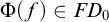 $\Phi (f)\in FD_0$
. We get a reduction
 $\Psi $
of D to the isomorphism relation on
 $\operatorname {FD}_0$
, where
 $\Psi (f)$
is the pair
 $(F,\Phi (f))$
.
The effective Borel hierarchy is closely tied to the hyperarithmetical hierarchy. In [Reference Hall, Knight and Lange8], it is observed that for any function
 $f\in 2^\omega $
and any computable ordinal
 $\alpha $
, the set
 $T_{\Sigma _\alpha }(f)$
(
 $T_{\Pi _\alpha }$
) of indices for effective
 $\Sigma _\alpha $
(
 $\Pi _\alpha $
) sets that contain f is
 $\Sigma ^0_\alpha $
(
 $\Pi ^0_\alpha $
), uniformly in f. In [Reference Hall, Knight and Lange8], this is used in some completeness proofs, and we shall use it here.
We turn to
 $\operatorname {TFAb}_1$
. In [Reference Knight and Saraph16], it is shown that for any computable subgroup of
 $\mathbb {Q}$
in which there is a computable set of primes that divide
 $1$
just finitely, but at least once, the set of indices for computable copies is m-complete
 $\Sigma ^0_3$
. One example of such a group is the subgroup G of
 $\mathbb {Q}$
generated by
 $\frac {1}{p}$
for primes p. It is easy to see that
 $I(G)$
is
 $\Sigma ^0_3$
. The completeness proof in [Reference Knight and Saraph16] involves showing that
 $Cof\leq _m I(G)$
. The computable reduction, defined on all
 $n\in \omega $
, gives a uniformly computable sequence of groups
 $(G_n)_{n\in \omega }$
such that
 $n\in Cof$
iff
 $G_n\cong G$
. Each
 $G_n$
is isomorphic to a subgroup of
 $\mathbb {Q}$
, in which each prime divides
 $1$
at most once, and in
 $G_n$
, the kth prime divides
 $1$
iff
 $k\in W_n$
.
Proposition 6.4. Let G be as above. Then the set
 $\text {Iso}(G)$
is complete effective
 $\Sigma _3$
. It is also complete X-effective
 $\Sigma _3$
for all X, and complete
 $\mathbf {\Sigma _3}$
.
Proof. Suppose
 $D\subseteq 2^\omega $
is effective
 $\Sigma _3$
, with index d. We need a computable reduction
 $\Phi $
of D to
 $\text {Iso}(G)$
. The set
 $T_{\Sigma _3}(f)$
is
 $\Sigma ^0_3$
relative to f, with index computed in a uniform way from f. Given
 $f\in 2^\omega $
, we relativize the construction from [Reference Knight and Saraph16], in a uniform way. Letting
 $Cof^f = \{n:W_n^f \text {is co-finite}\}$
, we get an f-computable sequence of groups
 $(G_{f,n})_{n\in \omega }$
, all in
 $\operatorname {TFAb}_1$
, such that
 $G_{f,n}\cong G$
iff
 $n\in Cof^f$
. The set
 $Cof^f$
is complete among
 $\Sigma ^0_3(f)$
sets, with reduction functions computed uniformly from f. In particular, knowing the index d for D, we can pass effectively from an index for
 $T_{\Sigma _3}(f)$
to a number
 $d'$
such that
 $d\in T_{\Sigma _3}(f)$
iff
 $d'\in Cof^f$
. All together, we have
 $f\in D$
iff
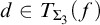 $d\in T_{\Sigma _3}(f)$
iff
 $d'\in Cof^f$
iff
 $G_{f,d'}\cong G$
. So, we take
 $\Phi (f)$
to be
 $G_{f,d'}$
.
The fact that
 $\text {Iso}(G)$
is effective
 $\Sigma _3$
implies that it is X-effective
 $\Sigma _3$
for all X, and it is
 $\mathbf {\Sigma _3}$
. To show that
 $\text {Iso}(G)$
is complete X-effective
 $\Sigma _3$
, we need, for each X-effective
 $\Sigma _3$
set D, an X-computable reduction
 $\Phi $
of D to
 $\text {Iso}(G)$
. We obtain
 $\Phi $
by relativizing the construction above. Moreover,
 $\Phi :2^\omega \rightarrow \operatorname {TFAb}_1$
.
Proposition 6.5. For
 $r> 0$
, each of the classes
 $\operatorname {TFAb}_r$
,
 $\operatorname {FD}_r$
contains a structure
 $\mathcal {A}$
for which
 $\text {Iso}(\mathcal {A})$
is complete effective
 $\Sigma _3$
, complete X-effective
 $\Sigma _3$
for all X, and complete
 $\mathbf {\Sigma _3}$
.
Proof. We consider the groups first. Let G be the group in the previous proposition. This is the structure we want in
 $\operatorname {TFAb}_1$
. For
 $r> 1$
, we have a
 $tc$
-embedding
 $\Psi $
of
 $\operatorname {TFAb}_1$
in
 $\operatorname {TFAb}_r$
. Let
 $\mathcal {A}$
be
 $\Psi (G)$
. We know that
 $\text {Iso}(\mathcal {A})$
is effective
 $\Sigma _3$
. For completeness, let D be an effective (X-effective)
 $\Sigma _3$
set. We have a computable (X-computable) reduction
 $\Phi $
of D to
 $\text {Iso}(G)$
, where
 $\Phi :2^\omega \rightarrow \operatorname {TFAb}_1$
. For
 $f\in 2^\omega $
, we have
 $f\in D$
iff
 $\Phi (f)\cong G$
iff
 $\Psi (\Phi (f))\cong \mathcal {A}$
. Thus,
 $\Psi (\Phi (f))$
is a computable (X-computable) reduction of D to
 $\text {Iso}(\mathcal {A})$
. Moreover, for all f,
 $\Psi (\Phi (f))$
is in
 $\operatorname {TFAb}_r$
. Thus,
 $\text {Iso}(\mathcal {A})$
is complete effective
 $\Sigma _3$
and complete X-effective
 $\Sigma _3$
. Every
 $\mathbf {\Sigma _3}$
set D is X-effective
 $\Sigma _3$
for some X, and our X-computable reduction of D to
 $\text {Iso}(\mathcal {A})$
is continuous. Therefore,
 $\text {Iso}(\mathcal {A})$
is also complete
 $\mathbf {\Sigma _3}$
.
We turn to the fields. Composing our
 $tc$
-embeddings of
 $\operatorname {TFAb}_1$
in
 $\operatorname {FD}_1$
and
 $\operatorname {FD}_n$
in
 $\operatorname {FD}_{n+1}$
, we arrive at a
 $tc$
-embedding
 $\Phi $
of
 $\operatorname {TFAb}_1$
in
 $\operatorname {FD}_r$
. Let
 $\mathcal {A} = \Phi (G)$
. Proceeding exactly as above, we get the fact that
 $\text {Iso}(\mathcal {A})$
is complete effective
 $\Sigma _3$
, complete X-effective
 $\Sigma _3$
, and complete
 $\mathbf {\Sigma _3}$
.
We turn to the isomorphism relation on the classes.
Proposition 6.6. For each
 $r> 0$
, the isomorphism relation on the classes
 $\operatorname {TFAb}_r$
,
 $\operatorname {FD}_r$
is complete effective
 $\Sigma _3$
. (It is also complete X-effective
 $\Sigma _3$
and complete
 $\mathbf {\Sigma _3}$
.)
Proof. We sketch the proof for
 $\operatorname {TFAb}_1$
. The proof for the other classes is the same. The class
 $\operatorname {TFAb}_1$
is effective
 $\Pi _2$
, and the isomorphism relation on
 $\operatorname {TFAb}_1$
is effective
 $\Sigma _3$
. For completeness, we use the fact that there is a specific group
 $G\in \operatorname {TFAb}_1$
for which
 $\text {Iso}(G)$
is complete effective (X-effective)
 $\Sigma _3$
, and that for each effective (X-effective)
 $\Sigma _3$
set D, we have a computable (X-computable) reduction
 $\Phi $
of D to
 $\text {Iso}(G)$
, such that
 $\Phi :2^\omega \rightarrow \operatorname {TFAb}_1$
. Let
 $\Psi (f) = (G,\Phi (f))$
. We have
 $f\in D$
iff
 $\Phi (f)\cong G$
, so
 $\Psi $
is a computable (X-computable) reduction of D to the isomorphism relation on
 $\operatorname {TFAb}_1$
. This shows that the isomorphism relation is complete effective (X-effective)
 $\Sigma _3$
. Take a set D that is
 $\mathbf {\Sigma _3}$
. This is X-effective
 $\Sigma _3$
for some X. Our X-computable reduction of D to
 $\text {Iso}(G)$
is continuous.
6.2 Non-embeddability
This section is devoted to proving a first step in answering the question of whether there exist
 $tc$
-reductions in the opposite direction, from
 $\operatorname {FD}_r$
to
 $\operatorname {TFAb}_r$
. Our result here will exclude functorial
 $tc$
-reductions for the case
 $r=1$
(indeed from
 $\operatorname {FD}_r$
to
 $\operatorname {TFAb}_1$
for each
 $r\geq 1$
) but it uses a specific fact about
 $\operatorname {TFAb}_1$
that fails for
 $r>1$
and also fails in every
 $\operatorname {FD}_r$
: an automorphism of a group in
 $\operatorname {TFAb}_1$
that fixes a single non-identity element must be the identity automorphism. Therefore, we remain uncertain whether this theorem can be extended to
 $\operatorname {TFAb}_r$
for
 $r>1$
, let alone whether it holds when
 $r>0$
and the condition of functoriality is dropped.
Theorem 6.7. For each
 $r>0$
, there is no functorial computable reduction from
 $\operatorname {FD}_r$
to
 $\operatorname {TFAb}_1$
.
Proof. Suppose that
 $(\Phi ,\Phi _*)$
were such a functorial reduction. Fix a presentation
 $A\in \operatorname {FD}_r$
of the purely transcendental extension
 $\mathbb {Q}(t_1,\ldots ,t_r)$
of the rationals. By functoriality
 $\Phi _*^{A\oplus \text {id}\oplus A}$
must be the identity map on
 $\Phi (A)$
, so fix an initial segment
 $\sigma $
of (the atomic diagram of) A sufficiently long that there exist three distinct elements
 $b_0,b_1,b_2\in \Phi (A)$
with
 $\Phi _*^{\sigma \oplus (\text {id}\upharpoonright |\sigma |) \oplus \sigma }(b_i)=b_i$
. It is consistent for us to extend
 $\sigma $
to the atomic diagram of a copy of
 $\mathbb {Q}$
. (This could fail for certain other fields in
 $\operatorname {FD}_r$
, but since
 $A\cong \mathbb {Q}(t_1,\ldots ,t_r)$
, it must hold.) Let
 $q_0,\ldots ,q_k\in \mathbb {Q}$
be all of the (finitely many) rational numbers mentioned in
 $\sigma $
when
 $\sigma $
is viewed as an initial segment of the diagram of this copy of
 $\mathbb {Q}$
, and let
 $a_i$
(for each
 $i\leq k$
) be the element of
 $\omega $
representing the rational
 $q_i$
in this copy.
Now, consider the following procedure for determining the relation of isomorphism on fields in
 $\operatorname {FD}_r$
. To get a contradiction, given any two fields
 $E,F\in \operatorname {FD}_r$
, we will reduce the question of whether
 $E \cong F$
to an effective
 $\Pi _2$
property. We use the atomic diagrams of
 $E,F$
to find the rationals
 $q_0,\ldots ,q_k$
in each. We construct a permutation
 $f_0$
of
 $\omega $
that is the identity on all but finitely many elements, but (for each i) maps the domain element of F representing
 $q_i$
to
 $a_i$
. Thus the field
 $F_0$
, built so that
 $f_0:F\to F_0$
is an isomorphism, has
 $\sigma $
as an initial segment of its atomic diagram, with the domain element
 $a_i\in F_0$
representing the rational
 $q_i$
for each i. We similarly construct an isomorphism
 $e_0$
mapping E onto another field
 $E_0$
with initial segment
 $\sigma $
.
Now we consider the two groups
 $G=\Phi (E_0)$
and
 $H=\Phi (F_0)$
in
 $\operatorname {TFAb}_1$
. Suppose
 $E\cong F$
. Then there exists an isomorphism
 $f:E_0\to F_0$
, and
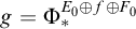 $g=\Phi _*^{E_0\oplus f\oplus F_0}$
will be a group isomorphism from G onto H. However,
 $E_0$
and
 $F_0$
both have initial segment
 $\sigma $
, and since each element
 $a_i$
mentioned in
 $\sigma $
represents the rational
 $q_i$
in both
 $E_0$
and
 $F_0$
, the isomorphism f must have
 $f(a_i)=a_i$
for all these i, namely,
 $\sigma \oplus (\text {id}\upharpoonright |\sigma |)\oplus \sigma \subset E_0\oplus f \oplus F_0$
. By our choice of
 $\sigma $
, the use of
 $\Phi _*^{A\oplus \text {id}\oplus A}(b_i) = b_i$
is
 $\sigma \oplus (\text {id}\upharpoonright |\sigma |)\oplus \sigma $
. Therefore
 $$ \begin{align*}g(b_i)= \Phi_*^{E_0 \oplus f \oplus F_0}(b_i) = \Phi_*^{\sigma\oplus(\text{id}\upharpoonright |\sigma|)\oplus \sigma}(b_i)=b_i\end{align*} $$
for each of the elements
 $b_0,b_1, b_2$
described earlier. Since g is an isomorphism, each of these elements
 $b_i$
individually satisfies
 $$ \begin{align*}(\forall \text{~prime powers~}p^m)~[((\exists x\in G)~p^mx=b_i) \iff (\exists y\in H)~p^my=g(b_i)],\end{align*} $$
hence, also satisfies
 $$ \begin{align} (\forall \text{~prime powers~}p^m)~[((\exists x\in G)~p^mx=b_i) \iff (\exists y\in H)~p^my=b_i]. \end{align} $$
Conversely, if
 $G,H\in \operatorname {TFAb}_1$
satisfy Equation 1 for both of these elements
 $b_i$
, then
 $G\cong H$
. (One of
 $b_0,b_1,b_2$
could be the identity element in G, and another could be the identity in H. However, as the three are distinct, the remaining element suffices to establish isomorphism between these rank-
 $1$
groups.) Since
 $\Phi $
is a Turing-computable embedding,
 $G\cong H$
implies
 $E\cong F$
, completing the converse. Thus
 $E\cong F$
if and only if Equation 1 holds for
 $b_0$
,
 $b_1$
, and
 $b_2$
.
Thus, we have effectively reduced the question of isomorphism between E and F to the
 $\Pi ^0_2$
property given above as Equation 1, using only finitely much information: the three elements
 $b_0,b_1,b_2$
, the rationals
 $q_0,\ldots ,q_k$
, and the elements
 $a_0,\ldots ,a_k$
of
 $\omega $
. This is impossible, since the isomorphism relation on
 $\operatorname {FD}_r$
is complete effective
 $\Sigma _3$
.
7 Countable reduction
In [Reference Miller, Cenzer, Porter and Zapletal20] the third author introduced the following definition of (computable)
 $\mu $
-ary reduction, an extension of a notion originally proposed in [Reference Miller and Ng21], by himself and Ng, in which
 $\mu $
was assumed to be finite.
Definition 7.1 [Reference Miller, Cenzer, Porter and Zapletal20, Definition 1.3].
Let E and F be equivalence relations on S and T. For any cardinal
 $\mu < |S|$
, we say a function
 $g:S^\mu \to T^\mu $
is a
 $\mu $
-ary reduction of E to F if for every
 $\vec {x} = (x_\alpha )_{\alpha \in \mu } \in S^\mu $
, we have
 $$ \begin{align*}\forall \alpha < \beta < \mu \ (x_\alpha E x_\beta \Leftrightarrow g_{\alpha}(\vec{x}) F g_{\beta}(\vec{x}))\end{align*} $$
where
 $g_\alpha $
is the
 $\alpha $
th component of g.
When
 $S \subseteq 2^\omega $
and
 $T\subseteq 2^\omega $
,
 $\mu \leq \omega $
, and g is computable, we write
 $E \le ^\mu _0 F$
and call this a computable
 $\mu $
-ary reduction.
In this section, we focus on computable countable reducibility, i.e., the case
 $\mu = \omega $
. Notice that when a Turing computable reduction exists, we automatically have a computable countable reduction. For example, the
 $tc$
-reduction
 $\Phi $
given in Proposition 5.1 yields a computable countable reduction
 $g:(\operatorname {FD}_0)^\omega \to (\operatorname {FD}_1)^{\omega }$
, where
 $$ \begin{align*}g(F_0,F_1,F_2,\ldots) = (\Phi(F_0),\Phi(F_1),\Phi(F_2),\ldots).\end{align*} $$
On the other hand, often a computable countable reduction exists even when there is no Turing computable reduction. We will see that under computable countable reducibility, all of the isomorphism relations on
 $\operatorname {TFAb}_r$
and
 $\operatorname {FD}_r$
are equivalent for all
 $r \ge 1$
, whereas Theorem 1.3 shows that the same fails to hold under Turing computable reducibility. In fact, Theorem 7.3 will show that, under computable countable reducibility, the isomorphism relation on
 $\operatorname {TFAb}_1$
has the maximal possible complexity for effective
 $\Sigma _3$
equivalence relations on
 $2^\omega $
. Intuitively this suggests that the non-reducibility results of Hjorth and Thomas (summarized as Theorem 1.3) do not stem from mere syntactic complexity, but instead depend intimately on the uncountable nature of the spaces in question. (If the universe were collapsed by a forcing extension, so that the original sets
 $\operatorname {TFAb}_r$
became countable, then the extension would contain a full computable reduction from each original
 $\operatorname {TFAb}_{r+1}$
to the preceding
 $\operatorname {TFAb}_r$
, given by the procedure in Theorem 7.3—although of course, in the extension, the original set
 $\operatorname {TFAb}_{r+1}$
would be superseded by a larger collection of torsion-free abelian groups of rank
 $r+1$
.)
Recall that
 $E_1$
is the equivalence relation on
 $2^\omega $
defined by two sets having all but finitely many of their columns being equal, namely
 $A E_1 B \iff \exists n \forall m\ge n, A^{[m]} = B^{[m]}$
, where
 $A^{[m]} = \{i \mid \langle m,i\rangle \in A\}$
is the m-th column of A.
 $E_2$
is the equivalence relation on
 $2^\omega $
defined by
 $A E_2 B \iff \sum _{n\in A \triangle B} \frac {1}{n+1} < \infty $
. In [Reference Miller, Cenzer, Porter and Zapletal20], it is shown that the equivalence relations
 $E_0, E_1, E_2$
are all
 $\Sigma ^0_2$
-complete under computable countable reduction.
Remark 7.2. Since we are working in the computable setting, the representation of structures does change the complexity. In particular, if
 $G\in \operatorname {TFAb}_r$
is represented as a subset of
 $\mathbb {Q}^r$
, then the divisibility predicate
 $n \mid g$
becomes computable (checking if
 $g/n\in G$
) and the complexity of the isomorphism becomes
 $\Sigma ^0_2$
(actually complete). However, in this paper, the structure are represented as free-standing structures, i.e., a point in
 $Mod(L)$
, thus the divisibility predicate is
 $\Sigma ^0_1$
and the complexity of isomorphism is
 $\Sigma ^0_3$
.
We now prove that the isomorphism relation on
 $\operatorname {TFAb}_1$
is
 $\Sigma ^0_3$
-complete under computable countable reduction. As a result, for every
 $r\ge 1$
, there is a computable countable reduction from the isomorphism relations of
 $\operatorname {FD}_r$
and
 $\operatorname {TFAb}_r$
to the isomorphism relation of
 $\operatorname {TFAb}_1$
. From here on, we abuse notation and write
 $\operatorname {TFAb}_r$
and
 $\operatorname {FD}_r$
to also mean the isomorphism relations on these classes.
Theorem 7.3.
 $\operatorname {TFAb}_1$
is
 $\Sigma ^0_3$
-complete under computable countable reducibility. More precisely, every
 $\Sigma ^0_3$
equivalence relation E on a subspace of
 $2^\omega $
is computably countably reducible to
 $\operatorname {TFAb}_1$
.
Proof. We first observe that
 $\operatorname {TFAb}_1$
is defined by the following computable infinitary
 $\Sigma ^0_3$
formula on a subset of
 $2^\omega $
: For
 $G,H\in \operatorname {TFAb}_1$
,
 $G\cong H$
if and only if
 $$ \begin{align*}\exists g\in G, h\in H, \forall q\in \mathbb{Q} [(\exists g'\in G~g' = qg) \Leftrightarrow (\exists h'\in H~h' = qh)].\end{align*} $$
Let E be a
 $\Sigma ^0_3$
equivalence relation on a subset of
 $2^\omega $
. We may assume that
 $AEB$
if and only if
 $\exists x \forall y \exists z R(A,B,x,y,z)$
where
 $R(A,B,x,y,z)$
is a computable predicate.
Recall that our reduction requires a Turing functional
 $\Phi $
that accepts as an oracle the join
 $A_0\oplus A_1\oplus \cdots $
of countably many sets in
 $2^\omega $
and (assuming every
 $A_n$
is in the field of the equivalence relation E) outputs the join
 $G_0\oplus G_1\oplus \cdots $
of the atomic diagrams of countably many groups in
 $\operatorname {TFAb}_1$
, so that
 $$ \begin{align*}(\forall n<m)~[A_m E A_n \iff G_m\cong G_n].\end{align*} $$
In the construction, we will consider each
 $G_i$
as a subgroup of
 $\mathbb {Q}$
. In fact,
 $\Phi $
will first build subgroups
 $G_i$
of
 $\mathbb {Q}$
, and then turn each of them into its atomic diagram.
Notice that for a given
 $m,n,k\in \omega $
, the property
 $\exists x\le k\ \forall y\ \exists z\ R(A_m,A_n,x,y,z)$
is uniformly
 $\Pi ^0_2$
. Thus, we can define chip functions
 $c_{m,n}$
, uniformly for all
 $m<n$
, that award infinitely many chips to
 $(m,n,k)$
just if
 $\exists x\le k\ \forall y\ \exists z\ R(A_m,A_n,x,y,z)$
, i.e., if there is some
 $x\le k$
witnessing
 $A_m E A_n$
. (Saying that
 $c_{m,n}$
awards a chip to
 $(m,n,k)$
at stage t means that
 $c_{m,n}(m,n,t) = k$
.) We will arrange these chip functions so that each
 $c_{m,n}$
has domain
 $ \{ \langle m,n,t\rangle : t\in \omega \} $
and image
 $\omega $
, with each element of
 $\omega $
lying in the domain of exactly one chip function. Finally, for convenience, we define
 $c_{n,m}=c_{m,n}$
whenever
 $m<n$
, taking advantage of the symmetric nature of E.
We now index the set of all prime numbers as
 $ \{ p_{m,n,k} : (m,n,k)\in \omega ^3~\&~m<n \} $
. In our construction, we aim to achieve the following:
-
• If
$(m,n,k)$
receives infinitely many chips, then
$1$
is infinitely divisible by
$p_{m,n,k}$
in both
$G_m$
and
$G_n$
. -
• if
$(m,n,k)$
receives only finitely many chips, then
$$ \begin{align*}(\exists r\in\omega) \left[\frac1{p_{m,n,k}^{r-1}}\in G_m~\&~\frac1{p_{m,n,k}^r}\notin G_m~\&~\frac1{p_{m,n,k}^r}\in G_n~\&~\frac1{p_{m,n,k}^{r+1}}\notin G_n\right]. \end{align*} $$


We give the procedure for each triple
 $(m,n,k)$
individually, as there is no interaction between any two such procedures, although the procedure here does involve other chip functions besides
 $c_{m,n}$
. Fix
 $(m,n,k)$
with
 $m<n$
, and write
 $p=p_{m,n,k}$
for simplicity, and fix
 $N=n+k$
. Every group
 $G_l$
contains
 $1$
, hence contains
 $\mathbb {Z}$
. The entire purpose of this procedure is to determine, for every group
 $G_l$
(not just
 $G_m$
and
 $G_n$
), which negative powers of p lie in
 $G_l$
. We will do this in such a way that, if
 $c_{m,n}$
awards finitely many chips to
 $(m,n,k)$
, then some power
 $p^{-r}$
with
 $r>0$
will lie in
 $G_n$
but not in
 $G_m$
; moreover, every
 $G_l$
will contain
 $p^{-(r-1)}$
and none will contain
 $p^{-(r+1)}$
. On the other hand, if
 $c_{m,n}$
awards infinitely many chips to
 $(m,n,k)$
, then every
 $G_l$
will contain every negative power of p. Thus this procedure makes sure that
 $G_m$
will be isomorphic to
 $G_n$
if and only if there is some x witnessing
 $A_m E A_n$
, but it will also do right by those
 $G_l$
with
 $l\leq N$
and
 $l\notin \{m,n\}$
, as described further down.
At stage
 $0$
, we define
 $p^{-1}$
to lie in
 $G_{n,0}$
. No negative power of p lies in any other
 $G_{l,0}$
, including
 $l=m$
. (Every
 $G_{l,0}$
contains
 $1$
, however.)
A stage
 $s+1$
with
 $c_{m,n}(s)=k$
is called a chip stage for
 $p_{m,n,k}$
. There is always a (least)
 $r>0$
with
 $p^{-r}\notin G_{m,s}$
: this r is the key exponent for
 $p_{m,n,k}$
at stage s. Every
 $G_{l,s}$
will contain
 $p^{-(r-1)}$
. The power
 $p^{-r}$
will lie in
 $G_{n,s}$
and many other
 $G_{l,s}$
, but not
 $G_{m,s}$
. No
 $G_{l,s}$
will contain
 $p^{-(r+1)}$
. We define the following linear order on the numbers
 $\leq N$
:
 $$ \begin{align*}m \prec n \prec 0\prec 1\prec\cdots\prec m-1\prec m+1\prec\cdots\prec n-1\prec n+1\prec\cdots\prec N-1\prec N\end{align*} $$
and follow these instructions at stage
 $s+1$
:
-
•
$p^{-r}$
enters every
$G_{l,s+1}$
, and
$p^{-(r+1)}$
enters
$G_{n,s+1}$
but not
$G_{m,s+1}$
. -
• For every
$l>N$
,
$p^{-(r+1)}$
enters
$G_{l,s+1}$
. -
• For each
$l\leq N$
with
$l\neq m$
and
$l\neq n$
, we find the greatest
$t_l\leq s$
(if any exists) such that
$(\exists j\prec l)c_{j,l}(t_l)\leq N$
. We then proceed through the
$\prec $
ordering. Already
$p^{-(r+1)}\in G_{n,s+1}$
but
$\notin G_{m,s+1}$
. For each subsequent l in turn (under
$\prec $
), enumerate
$p^{-(r+1)}$
into
$G_{l,s+1}$
if and only if
$p^{-(r+1)}$
was already enumerated into
$G_{j,s+1}$
, where
$c_{j,l}(t_l)\leq N$
. (If it exists, this j is unique, because
$t_l$
lies in the domain of only one chip function
$c_{j,l}$
.) If there was no such stage
$t_l$
, leave
$p^{-(r+1)}$
out of
$G_{l,s+1}$
.


Informally, the third bullet point says recursing on
 $\prec $
, each
 $G_l$
finds the chip function
 $c_{j,l}$
(with
 $j \prec l$
) that awarded a chip, and “follows”
 $G_j$
on whether or not
 $p^{-(r+1)}$
enters
 $G_l$
. Intuitively, this says that we decide whether
 $p^{-(r+1)}$
enters
 $G_l$
by considering the
 $G_j$
for which it seems most likely that
 $A_l E A_j$
based on the most recent
 $\Pi _2$
event (a chip being awarded).
Now, every
 $G_{l,s+1}$
contains
 $p^{-r}$
, but none contains
 $p^{-(r+2)}$
. At the next stage,
 $(r+1)$
will have replaced r as the key exponent for this p. This completes the instructions when
 $c_{m,n}(s)=k$
— but our procedure also has instructions to follow at the non-chip stages, i.e., those
 $s+1$
such that
 $c_{m,n}(s)\neq k$
.
At these non-chip stages
 $s+1$
, again we have a key exponent
 $r>0$
for p at stage s, with
 $p^{-r}\notin G_{m,s}$
. For this r,
 $p^{-r}$
lies in
 $G_{n,s}$
and also in many other
 $G_{l,s}$
, but none of these contains
 $p^{-(r+1)}$
. We use the same order
 $\prec $
as in the preceding paragraph, define
 $t_l$
the same way for each
 $l\leq N$
except for m and n themselves, and check whether
 $$ \begin{align*} & (\exists j\leq N)(\exists l\leq N)~[j\prec l~\&~l\neq n~\&~t_l\in\text{dom}(c_{j,l})~\&~((p^{-r}\notin G_{j,s}~\&~p^{-r}\in G_{l,s}) \\ &\quad \vee(p^{-r}\notin G_{l,s}~\&~p^{-r}\in G_{j,s}) )]. \end{align*} $$
(Notice that neither m nor n can serve as l here, since
 $j\prec l$
and
 $l\neq n$
.) If there are no such j and l, then we change nothing at this stage, because we already have
 $p^{-r}\in G_{l,s}$
if and only if
 $p^{-r}\in G_{j,s}$
with j being the
 $j \prec l$
for which it seems most likely that
 $A_l E A_j$
. However, if such j and l exist, then we repeat the procedure from above:
-
•
$p^{-r}$
enters every
$G_{l,s+1}$
, and
$p^{-(r+1)}$
enters
$G_{n,s+1}$
but not
$G_{m,s+1}$
. -
• For every
$l>N$
,
$p^{-(r+1)}$
enters
$G_{l,s+1}$
. -
• For each
$l\leq N$
with
$l\neq m$
and
$l\neq n$
, we proceed through the
$\prec $
ordering. Already
$p^{-(r+1)}\in G_{n,s+1}$
but
$\notin G_{m,s+1}$
. For each subsequent l in turn, enumerate
$p^{-(r+1)}$
into
$G_{l,s+1}$
if and only if
$p^{-(r+1)}$
was already enumerated into
$G_{j,s+1}$
, where
$c_{j,l}(t_l)\leq N$
. If there was no such stage
$t_l$
, leave
$p^{-(r+1)}$
out of
$G_{l,s+1}$
.





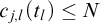


In this case, every
 $G_{l,s+1}$
now contains
 $p^{-r}$
, but none contains
 $p^{-(r+2)}$
. This completes this stage, and the construction.
Of course, each
 $G_l$
is the additive subgroup of
 $\mathbb {Q}$
generated by
 $\cup _s G_{l,s}$
, understanding that each
 $G_{l,s}$
will contain powers of many different primes
 $p_{m,n,k}$
, since we run the construction above for all triples
 $(m,n,k)$
with
 $m<n$
. We now prove the relevant facts about the construction.
Lemma 7.4. Fix any
 $(m,n,k)$
. If
 $c_{m,n}^{-1}(k)$
is infinite (so k received infinitely many chips from
 $c_{m,n}$
), then
 $1$
is divisible by every power of
 $p_{m,n,k}$
in every
 $G_l$
.
We will write “
 $p_{m,n,k}^{-\infty }\in G_l$
” to denote that every power
 $p_{m,n,k}^{-r}$
lies in
 $G_l$
. Of course this is just shorthand: there is no actual element
 $p_{m,n,k}^{-\infty }$
(and there is no finite stage s by which all of these powers have entered
 $G_{l,s}$
).
Proof. Every time k received a chip from
 $c_{m,n}$
, we adjoined new powers of
 $p_{m,n,k}$
to both
 $G_m$
and
 $G_n$
, and ensured that the power in
 $G_m$
also lies in every
 $G_l$
at that stage.
Notice, however, that even if k received only finitely many chips from
 $c_{m,n}$
, it is still conceivable that all powers of
 $p_{m,n,k}$
lie in every
 $G_l$
because the second part of the procedure was activated infinitely often. This could occur if there exist
 $l\in \omega $
and
 $k_0, k_1<N=n+k$
such that
 $c_{m,l}^{-1}(k_0)$
and
 $c_{n,l}^{-1}(k_1)$
are both infinite. In this case, the second part of the procedure may have been forced to increase the power r with
 $p^{-r}\in G_{m,s+1}$
at infinitely many stages s, as a new chip for
 $k_0$
from
 $c_{m,l}$
appeared, followed by a new chip for
 $k_1$
from
 $c_{n,l}$
, and then
 $k_0$
again, and so on. However, in this case,
 $k_0$
and
 $k_1$
guarantee (respectively) that
 $A_m E A_l$
and
 $A_l E A_n$
, so in fact
 $A_m E A_n$
in this case. So, while k itself may have received only finitely many chips from
 $c_{m,n}$
, some other
 $k'>k$
must have received infinitely many. We now state this possibility formally.
Lemma 7.5. The following are equivalent, for each
 $m<n$
and each k.
-
(1) For some l,
$p_{m,n,k}^{-\infty }\in G_l$
. -
(2) For every l,
$p_{m,n,k}^{-\infty }\in G_l$
.


Moreover, if these hold, then
 $A_m E A_n$
.
Proof. (2) trivially implies (1), and (1)
 $\implies $
(2) is clear from the construction for
 $(m,n,k)$
: at every stage s,
 $G_{n,s}$
is “ahead of”
 $G_{m,s}$
by one power of
 $p=p_{m,n,k}$
(meaning that there is some
 $r>0$
with
 $p^{-r}\in G_{n,s}-G_{m,s}$
, while
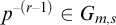 $p^{-(r-1)}\in G_{m,s}$
and
 $p^{-(r+1)}\notin G_{n,s}$
). Moreover, for every other l,
 $G_{l,s}$
is either “behind” with respect to powers of this p, i.e.,
 $G_{l,s}\cap \{ p^{-q} : q>0 \} =G_{m,s}\cap \{ p^{-q} : q>0 \} $
, or else “ahead” with respect to those powers, i.e.,
 $G_{l,s}\cap \{ p^{-q} : q>0 \} =G_{n,s}\cap \{ p^{-q} : q>0 \} $
. So, if any l at all has
 $p_{m,n,k}^{-\infty }\in G_l$
, then so do
 $G_n$
and
 $G_m$
and every other
 $G_j$
.
Suppose now that  . Say that a chip
 $c_{m,n}(s)$
is false if
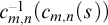 $c_{m,n}^{-1}(c_{m,n}(s))$
is finite. (That is, this chip has the potential to mislead us.) Fixing m, n, k, and
 $N=n+k$
, we see that there is some stage
 $s_0$
such that no
 $c_{j,l}$
with
 $j < l \leq N$
ever gives a false chip
 $c_{j,l}(s)$
to some
 $k' \le N$
at any stage
 $s\geq s_0$
, because there can only be finitely many such false chips given at all. Now let
 $s_1>s_0$
be a stage such that, for each
 $j<l \leq N$
and each
 $i\leq N$
with
 $c_{j,l}^{-1}(i)$
infinite, there is some s between
 $s_0$
and
 $s_1$
with
 $c_{j,l}(s)=i$
. Let
 $s_2>s_1$
be so large that this has happened again between
 $s_1$
and
 $s_2$
, and define
 $s_3<s_4<\cdots $
similarly. (One might say that the chip functions have dealt out a full round of true chips between each
 $s_q$
and
 $s_{q+1}$
.)
Since  , we know that
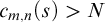 $c_{m,n}(s)>N$
(if
 $c_{m,n}(s)$
is defined) for every
 $s\geq s_0$
. Thus all subsequent stages in the procedure for
 $(m,n,k)$
are non-chip stages. We consider
 $l=0$
first (assuming
 $m\neq 0$
). If any
 $c_{0,m}^{-1}(i)$
with
 $i\leq N$
is infinite, then
 $c_{0,m}(s)=i$
for some s between
 $s_0$
and
 $s_1$
. But then
 $A_0E A_m$
, so
 . It follows that every
 $i'$
is a false chip for
 $c_{0,n}$
, and thus
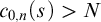 $c_{0,n}(s)>N$
for every
 $s\geq s_0$
. Therefore, by stage
 $s_1$
we will have
 $p_{m,n,k}^{-(r+1)}\notin G_{m,s_1}\cup G_{0,s_1}$
, according to the construction at the non-chip stage
 $s+1$
at which
 $c_{0,m}(s)=i$
, and
 $G_{0,s}$
will stay even with
 $G_{m,s}$
forever after (in terms of powers of
 $p_{m,n,k}$
), because
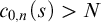 $c_{0,n}(s)>N$
for every
 $s\geq s_0$
, as shown above.
A similar argument shows that if any
 $c_{0,n}^{-1}(i)$
with
 $i\leq N$
is infinite, then
 $p_{m,n,k}^{-(r+1)}\in G_{n,s_1}\cap G_{0,s_1}$
, and
 $G_{0,s}$
will stay even with
 $G_{n,s}$
forever after (in terms of powers of
 $p_{m,n,k}$
). And if no
 $c_{m,0}^{-1}(i)$
nor any
 $c_{0,n}^{-1}(i)$
with
 $i\leq N$
is infinite, then both
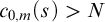 $c_{0,m}(s)>N$
and
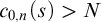 $c_{0,n}(s)>N$
for every
 $s\geq s_0$
, in which case either
 $G_{0,s}$
will stay even forever with
 $G_{m,s}$
(in case
 $G_{m,s_0}=G_{0,s_0}$
), or else it will stay even forever with
 $G_{n,s}$
(since then
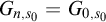 $G_{n,s_0}=G_{0,s_0}$
).
Finally, notice that if
 $m=0$
, then this same argument would hold with
 $1$
in place of
 $0$
(or with
 $2$
in place of
 $0$
, in case
 $n=1$
). It really shows that by stage
 $s_1$
, the next element
 $j_0$
after n in the
 $\prec $
-order must have linked its
 $G_{j_0}$
either to
 $G_m$
or to
 $G_n$
permanently (as far as powers of
 $p_{m,n,k}$
are concerned).
But now the same argument applies to the subsequent element
 $j_1$
in the
 $\prec $
-order, between the stages
 $s_1$
and
 $s_2$
. Once
 $j_0$
has “settled down” this way,
 $j_1$
will either select (by stage
 $s_2$
) which of m, n, and
 $j_0$
to link to, or else it will never link to any of them but will keep the same position that it holds at stage
 $s_1$
. In any case,
 $j_1$
never changes its position after stage
 $s_2$
. Continuing by induction, we see that after stage
 $s_N$
, the final element
 $j_{N-1}$
in the
 $\prec $
-order
 $m\prec n\prec j_0\prec \cdots \prec j_{N-1}$
on
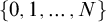 $\{0,1,\ldots ,N\}$
will have never change its position again. Thus, from stage
 $s_N$
on, no new powers of
 $p_{m,n,k}$
are ever added to
 $G_m$
or
 $G_n$
, or to any other
 $G_l$
. This proves the final claim of the lemma.
Lemma 7.6. If  , then
 $G_m\not \cong G_n$
.
Proof. By hypothesis, for every
 $k\in \omega $
,
 $c_{m,n}^{-1}(k)$
is finite. Lemma 7.5 shows that there are only finitely many powers of each
 $p_{m,n,k}$
in each
 $G_l$
, so (for a single fixed k) let r be maximal with
 $p_{m,n,k}^{-r}\in G_m$
, and fix the stage
 $s+1$
at which
 $p_{m,n,k}^{-r}$
was adjoined to
 $G_{m,s+1}$
. By the construction, we have
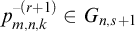 $p_{m,n,k}^{-(r+1)}\in G_{n,s+1}$
. Thus, for every k,
 $1$
is divisible by
 $p_{m,n,k}^{(r+1)}$
in
 $G_n$
(for the r corresponding to this k), but not in
 $G_m$
. It follows that
 $G_m\not \cong G_n$
.
Lemma 7.7. If
 $A_m E A_n$
, then
 $G_m\cong G_n$
.
Proof. For every
 $m'<n'$
and every i, Lemma 7.4 shows that
 $$ \begin{align*}p_{m',n',i}^{-\infty}\in G_m \iff p_{m',n',i}^{-\infty}\in G_n.\end{align*} $$
In particular, if k is the least such that
 $c_{m,n}^{-1}(k)$
is infinite, then for every
 $i\geq k$
,
 $p_{m,n,i}^{-\infty }$
lies in both
 $G_m$
and
 $G_n$
. For the remaining finitely many i, there will be powers r (likely distinct for different i) such that
 $p_{m,n,i}^{-r}$
lies in
 $G_n$
but not
 $G_m$
(assuming without loss of generality that
 $m<n$
). Recall that, to show
 $G_m\cong G_n$
, we need to show that there are only finitely many prime powers
 $p^{-r}$
that lie in one of
 $G_m$
and
 $G_n$
but not in the other, so these finitely many values
 $i<k$
do not upset us. (The initial result made it clear that
 $p_{m,n,i}^{-\infty }$
lies in neither
 $G_m$
nor
 $G_n$
, so these i really do yield only finitely many such prime powers.)
However, there are many more primes to be considered. We claim that for those primes
 $p_{m',n',k'}$
with
 $(m',n')\neq (m,n)$
and
 $n'+k'=N'\geq \max (n,k)$
, each power
 $p_{m',n',k'}^r$
will lie in
 $G_m$
if and only if it lies in
 $G_n$
. Recall our convention that
 $m'<n'$
in all these triples, so there are only finitely many triples
 $(m',n',k')$
with
 $n'+k'<\max (n,k)$
. Consequently, this claim, once proven, will suffice to show that
 $G_m\cong G_n$
.
The claim holds because there are infinitely many s with
 $c_{m,n}(s)=k$
. Each such stage
 $s+1$
is a non-chip stage in the procedure for
 $(m',n',k')$
, because
 $\text {dom}(c_{m,n})\cap \text {dom}(c_{m',n'})=\emptyset $
when
 $(m,n)\neq (m',n')$
. With
 $m<n\leq N'$
and
 $k\leq N'$
, the procedure for
 $(m',n',k')$
at stage
 $s+1$
will set
 $t_n=s$
, the greatest stage
 $\leq s$
at which some
 $j\prec n$
(namely m) has
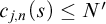 $c_{j,n}(s)\leq N'$
. Using the key exponent r at this stage, this procedure will ask whether
 $$ \begin{align*}(p_{m',n',k'}^{-r}\in G_{m,s} \iff p_{m',n',k'}^{-r}\in G_{n,s}).\end{align*} $$
If not, it will increase the key power by
 $1$
, to
 $r+1$
, and ensure that
 $$ \begin{align*}(p_{m',n',k'}^{-(r+1)}\in G_{m,s} \iff p_{m',n',k'}^{-(r+1)}\in G_{n,s}).\end{align*} $$
(Whether this power is in both these sets or out of them both depends on
 $t_m$
; this is irrelevant to our argument here.) If
 $G_{m,s}$
and
 $G_{n,s}$
were “even” with respect to this prime, it is still possible that the procedure will increase the key power on account of
 $t_l$
for some other
 $l\leq N'$
. But even if it does so, since there are infinitely stages s in
 $c_{m,n}^{-1}(k)$
, and at some later stage
 $s \in c_{m,n}^{-1}(k)$
we will “catch up” and again have
 $$ \begin{align*}(p_{m',n',k'}^{-(r+1)}\in G_{m,s} \iff p_{m',n',k'}^{-(r+1)}\in G_{n,s}).\end{align*} $$
Thus, for every power r,
 $p_{m',n',k'}^{-r}$
lies in
 $G_m$
if and only if it lies in
 $G_n$
. As noted above, this completes the proof.
By Lemmas 7.6 and 7.7, our procedure
 $\Phi $
does indeed compute a countable reduction from E to
 $\operatorname {TFAb}_1$
.
Corollary 7.8. Uniformly for each
 $d>0$
, there is a computable countable reduction from the space
 $\operatorname {FD}_d$
of fields of transcendence degree d over
 $\mathbb {Q}$
to the space
 $\operatorname {TFAb}_1$
of torsion-free abelian groups of rank
 $1$
.
Proof. Note that the isomorphism problem on
 $\operatorname {FD}_d$
is uniformly
 $\Sigma ^0_3$
via
 $$ \begin{align*} F \cong E \Leftrightarrow \exists \bar a\in F, \bar b \in E~[ & (\bar a\text{ is an algebraically independent }d\text{-tuple})\\ &\wedge(\bar b\text{ is an algebraically independent }d\text{-tuple})\\ &\wedge(\bar a\mapsto \bar b\text{ extends to an isomorphism }F \to E)]. \end{align*} $$
Thus, by the previous Theorem 7.3, there is a uniform computable countable reduction from
 $\operatorname {FD}_d$
to
 $\operatorname {TFAb}_1$
.
Since the isomorphism relation on
 $\operatorname {TFAb}_r$
is similarly
 $\Sigma ^0_3$
, uniformly in r, we have a similar corollary for groups, which contrasts with Theorem 1.3 of Hjorth and Thomas.
Corollary 7.9. Uniformly for each
 $r\geq 0$
, there is a computable countable reduction from the space
 $\operatorname {TFAb}_r$
of torsion-free abelian groups of rank r to the space
 $\operatorname {TFAb}_1$
.
Acknowledgments
The authors would like to thank Phillip Dittman, Matthew Harrison-Trainor, Vincent Ye, and Arno Fehm for a useful discussion that led to the proof in Section 5.
Funding
This material is based on work supported by the National Science Foundation under Grant #DMS-1928930 while the authors participated in programs hosted by the Mathematical Sciences Research Institute in Berkeley, CA, during Fall 2020 and Summer 2022. The first author acknowledges support from the National Science Foundation under Grant #DMS-2054558. The second author acknowledges support from the National Science Foundation under Grant #DMS-1800692. The third author acknowledges support from the Simons Foundation under Grant #581896, from the National Science Foundation under Grant #DMS-2348891, and from several grants by The City University of New York PSC-CUNY Research Award Program.



