1. Introduction
Automated guided vehicle (AGV) is widely used in the fields of intelligent logistics, intelligent manufacturing, and warehouse management, and one of its core problems is efficient and reliable path planning [Reference Dash, Parhi, Muni and Das1]. Traditional path planning methods, such as the A* algorithm [Reference Wang, Yang, Huang and He2] and Dijkstra’s algorithm [Reference Su, Wu and Li3], perform well in simple structured environments, but struggle in complex environments [Reference Vlachos, Martinez, George, panagiotis and Mihalis4]. Sampling-based algorithms, especially the rapid exploratory randomized tree (RRT) algorithm [Reference Zhang, Gao, Wang, Zhao, Wu and p.5], offer a promising solution due to their probabilistic completeness and adaptability to complex environments. However, the standard RRT* algorithm [Reference Maza6] is slow to converge, has excessive path oscillations, and is poorly adapted to dynamic environments, limiting its direct application to real-world AGV navigation.
In terms of AGV path planning, the traditional RRT* algorithm has a weak local search capability and may be prone to fall into local optimal solutions in complex environments, making it difficult to quickly find the globally optimal path [Reference Wang, Zhao and Tang7]. The generated paths may not be the optimal geometric paths, and there may be some twists and turns or unnecessary turns, which can satisfy the passage requirements from the starting point to the end point, but are not optimal in terms of path length and other indicators, which is not conducive to the efficient operation of the AGVs and the saving of energy consumption [Reference Wei, Bai and Lu8].
In this paper, an improved APF-QRRT* algorithm is proposed. The improved APF-QRRT* algorithm obtains a set of discrete critical path points connecting the start point and the end point through the Q-RRT* algorithm, and then fine-tunes the paths by using the local optimization ability of the APF, and fine-tunes the paths by using the local optimization ability of the APF algorithm to achieve obstacle avoidance, and to improve the path smoothing and security. The traditional Q-RRT* algorithm is improved, and the fast alternating expansion of two random trees is realized by introducing the two-way search strategy of two random trees and adopting the node greedy expansion, which tries to take the node closest to the vector tree as the reference of this tree expansion during the iterative process of path node generation. This strategy can greatly improve the search efficiency of the algorithm in multiple environments and the safety of path planning.
2. RRT* algorithm
2.1. Basic principles of RRT* algorithm
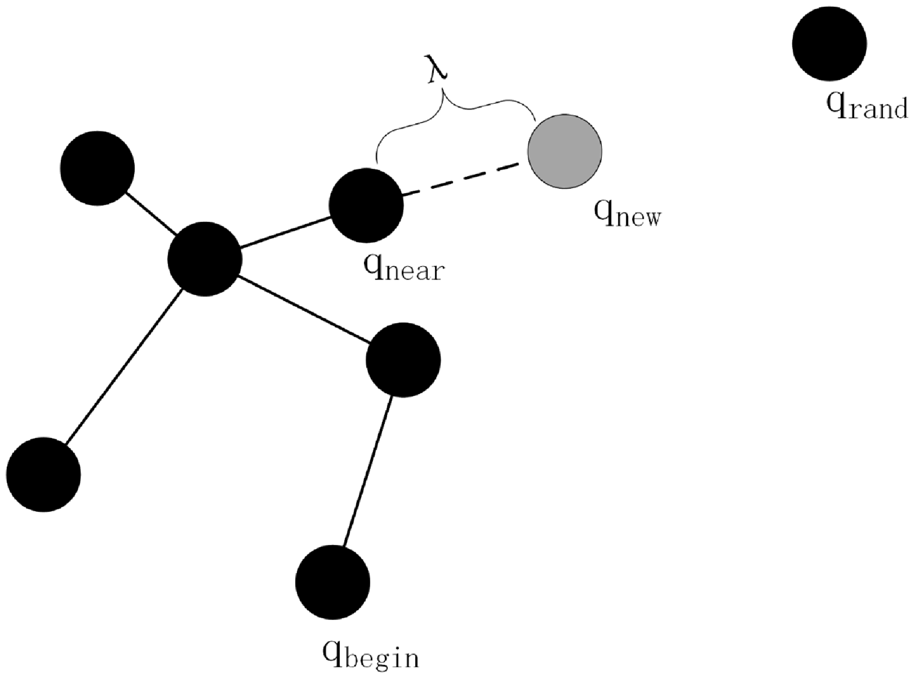
The RRT algorithm is a sampling-based path planning algorithm that explores the space by randomly sampling an extended tree structure to find a path from a starting point to a goal point. Its core advantage is that it can quickly generate feasible paths in high-dimensional spaces, but the generated paths are usually not optimal [Reference Lei, Li, Gao, Xue and Song9]. Assuming that the robot’s starting position is
 $q_{\textit{begin}} , q_{rand}$
is a random sampling point in the space,
 $q_{near}$
is the nearest node to
 $q_{rand}$
in the random tree, the new node obtained after expanding in a straight line between
 $q_{near}$
and
 $q_{rand}$
with step
 $\lambda$
is
 $q_{new}$
, and the ending position is
 $q_{end}$
. The single-step expansion of the RRT algorithm is shown in Figure 1.
Single-step expansion diagram of the RRT algorithm.

The RRT* algorithm introduces the following optimization mechanism based on the RRT algorithm:
(1) Path cost optimization:
RRT* continuously evaluates and optimizes the cost of paths (e.g., path length, energy consumption, etc.) during tree expansion to find better paths [Reference Ganesan, Ramalingam and Mohan10].
The goal of RRT* is to minimize the path cost from the starting point to each node. Assuming that the path cost from the starting point
 $q_{init}$
to node
 $q$
is
 $C(q)$
, the cost function can be expressed as:
 \begin{equation} C\left(q\right)=C\left(q_{\text{parent}}\right)+\text{Cost}\left(q_{\text{parent}},q\right) \end{equation}
where
 $C(q_{\text{parent}})$
is the path cost from the starting point to the parent node
 $q_{\text{parent}}$
and
 $\text{Cost}(q_{\text{parent}},q)$
is the path cost from the parent node
 $q_{\text{parent}}$
to the current node
 $q$
.
(2) Neighboring node reconnection:
Each time a new node is expanded, RRT* checks the neighboring nodes and tries to optimize the paths of the neighboring nodes through the new node [Reference Liu, Hu, Wei, p. Guo and Zhang11].
The set of neighboring nodes
 $Q_{near}$
is the set of nodes within a certain distance from the new node
 $q_{new}$
. It is defined by the following equation:
 \begin{equation} Q_{near}=\left\{q\in T|\textit{Distance}\left(q,q_{near}\right)\leq r\right\} \end{equation}
where
 $\textit{Distance}(q,q_{new})$
is the distance between node
 $q$
and the new node
 $q_{new}$
.
 $r$
is the search radius, which is usually related to the node density and spatial dimension of the tree. The choice of neighborhood radius
 $r$
directly affects the performance of the algorithm. If
 $r$
is too small, the optimal parent node may not be found; if
 $r$
is too large, the computational complexity will increase.
For each neighboring node
 $q\in Q_{near}$
, RRT* tries to optimize its path cost through a new node
 $q_{new}$
. If the path cost of
 $q_{new}$
can be reduced through
 $q$
, its parent node is updated to
 $q_{new}$
. The formula is as follows:
 \begin{equation} if\, C\left(q_{new}\right)+Cost\left(q_{new},q\right)\lt C\left(q\right)\Rightarrow q_{\textit{parent}}=q_{new} \end{equation}
where
 $C(q_{new})$
is the path cost from the starting point to the new node
 $q_{new}$
.
 $\mathrm{Cos}t(q_{new},q)$
is the path cost from the new node
 $q_{new}$
to the neighboring node
 $q$
.
 $C(q)$
is the path cost from the starting point to the neighboring node
 $q$
.
(3) Parent node reselection:
For a newly expanded node, RRT* tries to reselect its parent node to reduce the total cost from the starting point to that node [Reference Dong, Wang, Fang, Ran and Liu12].
When expanding a new node
 $q_{new}$
, RRT* selects a node from the set of neighboring nodes
 $Q_{near}$
as its parent node to minimize the cost of the path from the start point to
 $q_{new}$
. The formula is as follows:
 \begin{equation} q_{\text{parent}}^{*}=argmin_{q\in {Q_{\text{neat}}}}\left(C\left(q\right)+\text{Cost}\left(q,q_{\mathrm{new}}\right)\right) \end{equation}
where
 $q_{\textit{parent}}^{\ast }$
is the optimal parent node that minimizes the path cost.
 $C(q)$
is the path cost from the starting point to node
 $q$
.
 $\mathrm{Cos}t(q_{new},q)$
is the path cost from node
 $q$
to the new node
 $q_{new}$
.
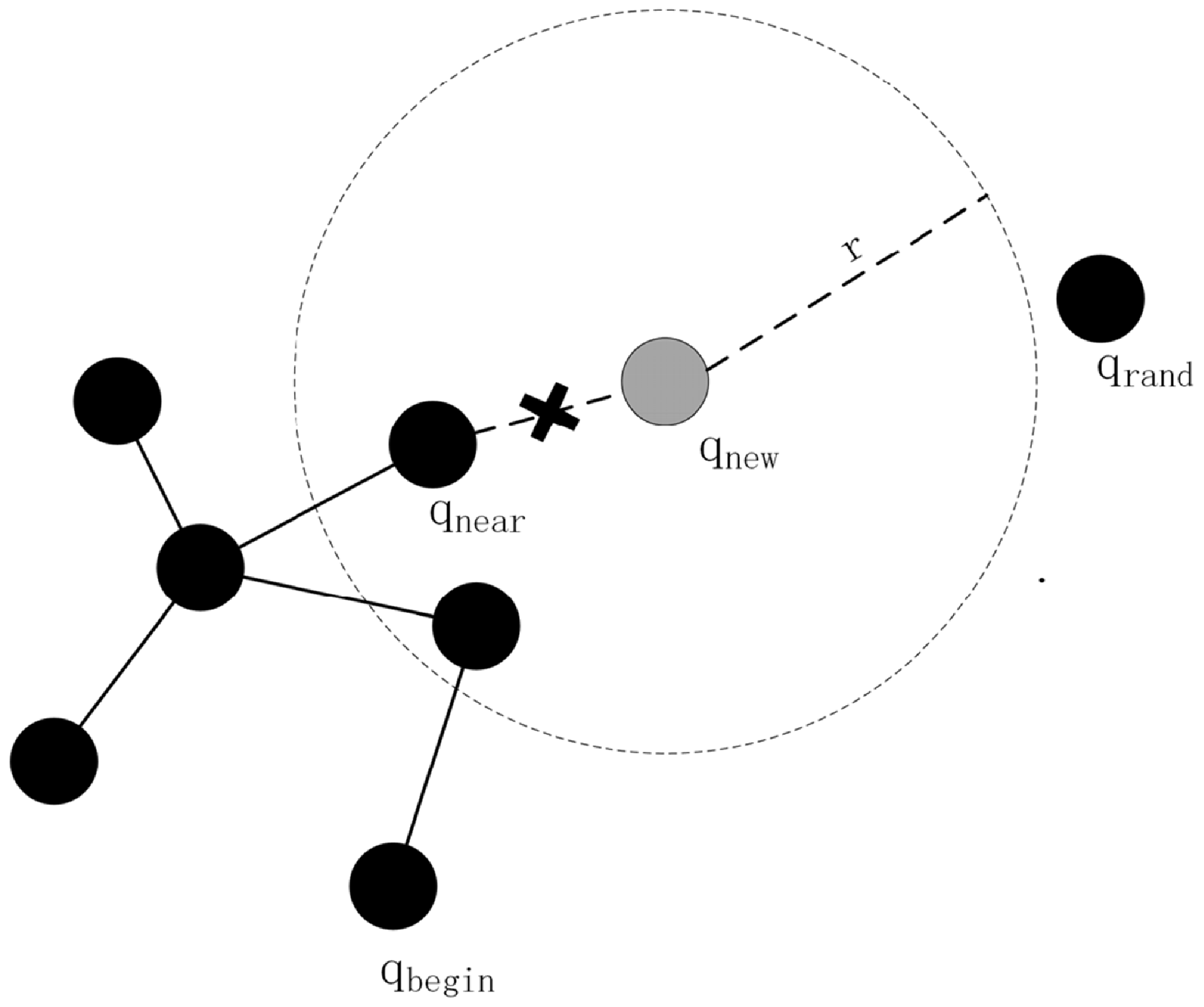
The single-step expansion process of the RRT* algorithm is shown in Figure 2.
RRT* algorithm single-step expansion diagram.

Reselect the parent node:Determine the set of leaf nodes within the radius
 $r$
with the new node
 $q_{new}$
as the center of the circle, calculate the path lengths from the starting position
 $q_{\textit{begin}}$
to the new node
 $q_{new}$
via the nodes in the set of leaf nodes in turn, and select the leaf node with the shortest path length as the parent node of the new node
 $q_{new}$
. Rewiring:Disconnect the new node
 $q_{new}$
from the original parent node
 $q_{near}$
, and connect the new node
 $q_{new}$
to the new parent node.
2.2. Basic principle of Q-RRT* algorithm
The core advantage of the RRT* algorithm is that it can quickly generate feasible paths in high-dimensional spaces, but the generated paths are usually not optimal [Reference Zhang, Wang, Guo, Han and Zhang13]. To address this issue, existing research has introduced the value function (Q-value) into the RRT* algorithm.
The value function
 $Q(q)$
is used to evaluate the potential value of node
 $q$
and usually combines the following two parts:
Path cost: path cost
 $\mathrm{Cos}t(q)$
from the starting point to node
 $q$
; Heuristic information: heuristic estimation
 $h(q)$
from node
 $q$
to the goal point. The formula is as follows:
 \begin{equation} Q\left(q\right)=\alpha \cdot Cost\left(q\right)+\beta \cdot h\left(x\right) \end{equation}
where
 $\alpha$
and
 $\beta$
are weight parameters to balance the path cost and heuristic information.During random sampling, high-value regions are prioritized for sampling. This is realized by a probability distribution:
 \begin{equation} P\left(q_{\text{rand}}\right)\propto Q\left(q_{\text{rand}}\right) \end{equation}
The probability that
 $q_{rand}$
random point a is selected is proportional to its value
 $Q(q_{rand})$
.
In selecting the parent node, not only the path cost is considered but also the value function is introduced:
 \begin{equation} q_{\text{parent}}=argmin_{q\in {q_{\text{near}}}}\left(\text{Cost}\left(q\right)+\|q-q_{\mathrm{new}}\|+\gamma \cdot Q\left(q\right)\right) \end{equation}
where
 $\gamma$
is the weight parameter of the value function.
The value function is used to evaluate potential optimization paths during rewiring:
 \begin{equation} \text{if Cost}\left(q_{\mathrm{new}}\right)+\|q_{\mathrm{new}}-q_{\text{near}}\|+\gamma \cdot Q\left(q_{\mathrm{new}}\right)\lt \text{Cost}\left(q_{\text{near}}\right),\text{then }q_{\text{near}}.\text{parent}=q_{\mathrm{new}} \end{equation}
Considering the ancestor nodes on the basis of the Q-RRT* algorithm, the cost function is optimized with the principle of triangular inequality (in the Euclidean distance field, the commonly used cost function usually satisfies the triangular inequality), and if the paths are collision-free, the ancestor node of the node will become the critical path point [Reference Tengesdal, Pedersen and Johansen14]. In Figure 3(a), traverse the ancestor nodes to get the set of ancestor nodes, take the ancestor node
 $q_{new}$
in the set as the new parent node and compute the path cost from the ancestor node to
 $q_{new}$
until the ancestor node with the optimal path cost is found, and take the ancestor node as the new parent node of
 $q_{new}$
. In Figure 3(b), the ancestor node is used as the new parent node of
 $q_{new}$
, and the path cost from the ancestor node to
 $q_{near}$
is calculated and judged whether the path cost is less than the original path cost, and then choose whether to update the ancestor node as the new parent node of
 $q_{near}$
.
Schematic diagram of the Q-RRT * algorithm. (a) is the graph of the Q-RRT * algorithm for re-selecting parent nodes; (b) is the graph of the Q-RRT * algorithm for rewiring.

3. Improved Q-RRT* algorithm
3.1. Search strategies based on a two-way search
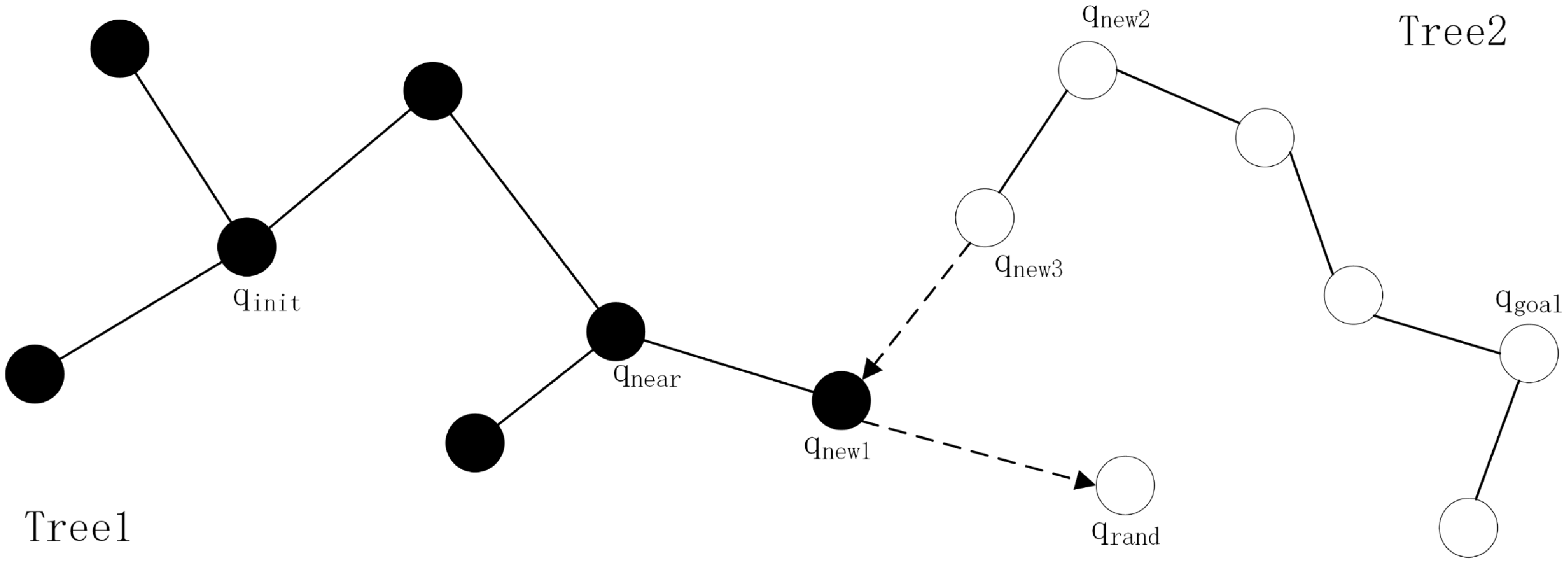
The traditional Q-RRT* algorithm rewiring mechanism and the parent node selection process increase the computational complexity, especially when the number of nodes is large, the algorithm runs for a long time. The asymptotic optimality of Q-RRT* implies that it needs a long running time to find a high-quality path, and the initial paths may be long [Reference Adibeli, Liu, Chao and Awodi15]. To address this problem, this paper introduces two random trees bi-directional search and adopts node greedy expansion. In the iterative process of path node generation, we try to use the nearest node of the pairwise tree as a reference for the expansion of this tree, to realize the fast alternate expansion of the two trees. The bidirectional search node expansion principle of the Q-RRT* algorithm is illustrated in Figure 4.
In the initialization phase, two node ensembles containing the starting point and the end point are defined, respectively, and at each iteration, the nearest point
 $q_{near}$
in the tree is selected by sampling a random point
 $q_{rand}$
in the state space, and if there is no collision between
 $q_{rand}$
and
 $q_{near}$
, a new node
 $q_{near1}$
is generated from the expansion with a certain step length of
 $q_{near}$
. Subsequently, another search tree adopts the greedy strategy and expands in a straight line toward the target point
 $q_{near1}$
until it encounters an obstacle or a newly generated node
 $q_{new3}=q_{new1}$
. If the two search trees are connected, it means that a feasible path is found and the program is finished; otherwise, the next iteration is performed until the end condition is reached. The specific formula of the algorithm after improving the search strategy is expressed as follows.
Node expansion graph of Q-RRT* algorithm for bidirectional search.

3.2. Improved Q-RRT* algorithm strategy flow
Initialization:
 \begin{equation} T_{a}=\left\{q_{\text{start}}\right\},\,\,\,\enspace T_{b}=\left\{q_{\text{goal}}\right\} \end{equation}
Sampling:
 \begin{equation} q_{\text{rand}}=\text{Sample}\left(\right) \end{equation}
Extended tree
 $T_{a}$
:
 \begin{align} q_{{\text{near}_{a}}}=argmin_{q\in {T_{a}}}\|q-q_{\text{rand}}\| \\[-25pt] \nonumber \end{align}
 \begin{equation*} q_{{\mathrm{new}_{a}}}=\text{Steer}\left(q_{{\text{near}_{a}}},q_{\text{rand}}\right) \end{equation*}
If
 $\text{CollisionFree}(q_{{\text{near}_{a}}},q_{{\mathrm{new}_{a}}})$
, then
 $q_{ne{w_{a}}}$
adds
 $T_{a}$
to it:
 \begin{equation} T_{a}=T_{a}\cup \left\{q_{{\mathrm{new}_{a}}}\right\} \end{equation}
Apply Q-RRT* rewiring:
 \begin{equation} Q_{{\text{near}_{a}}}=\left\{q\in T_{a}|\|q-q_{{\mathrm{new}_{a}}}\|\leq r\right\} \end{equation}
For each
 $q\in Q_{ner{a_{a}}}$
:
 \begin{equation} \begin{array}{ll} \mathrm{if} & \text{Cost}\left(q_{{\mathrm{new}_{a}}}\right)+\|q-q_{{\mathrm{new}_{a}}}\|\lt \text{Cost} \end{array}\left(q\right)\, \text{then}\, \text{UpdateParent}\left(q,q_{{\mathrm{new}_{a}}}\right) \end{equation}
Try to connect the tree
 $T_{b}$
:
 \begin{align} q_{{\text{near}_{b}}}=argmin_{q\in {T_{b}}}\|q-q_{{\mathrm{new}_{a}}}\| \\[-25pt] \nonumber \end{align}
 \begin{equation*} q_{{\mathrm{new}_{b}}}=\text{Steer}\left(q_{{\text{near}_{b}}},q_{{\mathrm{new}_{a}}}\right) \end{equation*}
If
 $q_{{\mathrm{new}_{b}}}=q_{{\mathrm{new}_{a}}}$
, the two trees are connected successfully:
 \begin{equation} \begin{array}{l} \text{Path}=\text{ConstructPath}\left(T_{a},T_{b}\right) \end{array} \end{equation}
Swap tree:
 \begin{equation} \mathrm{T}_{\mathrm{a}},\mathrm{T}_{\mathrm{b}}=\mathrm{T}_{\mathrm{b}},\mathrm{T}_{\mathrm{a}} \end{equation}
Termination conditions:
 \begin{align} \mathrm{if}\,\enspace \text{Path}\neq \mathrm{\varnothing }\,\enspace \mathrm{or}\,\,\text{Iterations}\geq \text{MaxIterations}\,\text{then}\,\text{Terminate} \end{align}
Compared with the traditional Q-RRT* algorithm, this paper makes an improvement to the search strategy. The specific process of the improved Q-RRT* algorithm described in this paper is shown in Figure 5.
3.3. Validation of improved Q-RRT* algorithm
The MATLAB software is used to simulate the improved Q-RRT* algorithm as well as the traditional Q-RRT* algorithm and to compare the above two algorithms by the path planning time and the number of nodes expanded during the path planning process, in which the running graph of the traditional Q-RRT* algorithm is shown in Figure 6(a) and the running graph of the improved Q-RRT* algorithm is shown in Figure 6(b).
Flowchart of the improved Q-RRT* algorithm.

Schematic diagram of Q-RRT* algorithm path planning results. (a) The traditional Q-RRT* algorithm; (b) The improved Q-RRT* algorithm.

As shown in Table I, the improved Q-RRT* algorithm reduces path planning time by 15.95% compared to the traditional Q-RRT* algorithm. Regarding node scalability, the improved algorithm achieves a 43.54% reduction in node count compared to the traditional algorithm. In terms of path planning success rate, the improved Q-RRT* algorithm demonstrates a 9% increase. This demonstrates that the improved Q-RRT* algorithm achieves significant operational efficiency gains over the traditional Q-RRT* algorithm, while also validating the effectiveness of the enhanced bidirectional search strategy.
4. Algorithmic fusion
4.1. Artificial potential field method
The artificial potential field method (APF) is a classical algorithm for robot path planning. Its core idea is to abstract the robot’s motion environment as a potential field, where the target point exerts an attractive force on the robot and the obstacle exerts a repulsive force on the robot, and the robot moves by being subjected to these forces, thus realizing obstacle avoidance and navigation [Reference Li, Wu, Li and Wang16].
The gravitational potential field
 $Uatt(q)$
is a function of the distance from the robot’s current position
 $q$
to the target point
 $q_{goal}$
, defined as follows:
 \begin{equation} U_{att}\left(q\right)=\frac{1}{2}k_{att}\cdot d\left(q,q_{goal}\right)^{2} \end{equation}
where
 $k_{att}$
is the gravitational coefficient (positive), which controls the strength of the gravitational field.
 $d(q,q_{goal})$
is the Euclidean distance from the robot’s current position
 $q$
to the target point
 $q_{goal}$
:
 \begin{equation} \mathrm{d}\left(q,q_{goal}\right)=\parallel q-q_{goal}\parallel \end{equation}
The gravitational formula is as follows:
The gravitational force
 $Fatt(q)$
is the negative gradient of the gravitational potential field:
 \begin{equation} F_{att}\left(q\right)=-\nabla U_{att}\left(q\right)=-k_{att}\cdot \left(q-q_{goal}\right) \end{equation}
The gravitational force is directed toward the target point and is proportional in magnitude to the distance.
The repulsive potential field
 $U_{rep}$
is a function of the distance between the robot and the obstacle and is defined as follows:
 \begin{equation} U_{rep}\left(q\right)=\left\{\begin{array}{ccc} \frac{1}{2}k_{rep}\left(\frac{1}{d\left(q,q_{obs}\right)}-\frac{1}{d_{0}}\right)^{2}, & if\, d\left(q,q_{obs}\right)\leq d_{0} & \\ 0, & if\, d\left(q,q_{obs}\right)\gt d_{0} & \end{array}\right. \end{equation}
where
 $k_{rep}$
is the repulsive force coefficient (positive), which controls the strength of the repulsive field.
 $d(q,q_{obs})$
is the distance from the robot’s current position
 $q$
to the obstacle.
 $d_{0}$
is the range of the repulsive field, which is 0 when the distance is greater than
 $d_{0}$
.
 \begin{equation} F_{rep}\left(q\right)=\left\{\begin{array}{ccc} k_{rep}\left(\frac{1}{d\left(q,q_{obs}\right)}-\frac{1}{d_{0}}\right)\cdot \frac{\left(q-q_{obs}\right)}{d\left(q,q_{obs}\right)^{3}}, & if\, d\left(q,q_{obs}\right)\leq d_{0} & \\ 0, & if\, d\left(q,q_{obs}\right)\gt d_{0} & \end{array}\right. \end{equation}
The formula for repulsive force is as follows.
Comparison of path planning performance between two algorithms.

The direction of the repulsive force is away from the obstacle, and its magnitude is inversely proportional to the distance.
The combined force
 $F(q)$
is the vector sum of the gravitational force
 $Fatt(q)$
and the repulsive force
 $F_{rep}(q)$
.
 \begin{equation} {F}\left(q\right)={F}_{att}\left(q\right)+{F}_{rep}\left(q\right) \end{equation}
The robot moves in the direction of the combined force.
The motion of the AGV is determined by the combined force
 $F(q)$
and its position is updated as follows:
 \begin{equation} q\leftarrow q+\eta \cdot \frac{F(q)}{\|F(q)\|} \end{equation}
where
 $\eta$
is the step coefficient, which controls the movement speed of the robot.
 $\frac{F\left(q\right)}{\parallel F\left(q\right)\parallel }$
is the unit direction vector of the combined force.
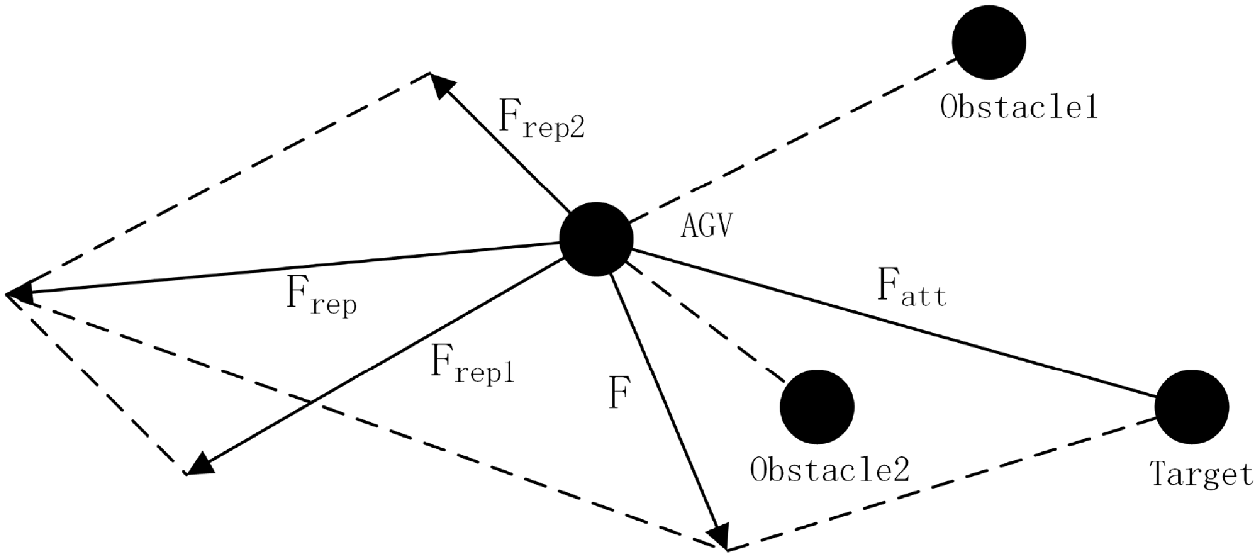
AGV force analysis diagram.

Flowchart of the fusion navigation algorithm.

The schematic diagram of the resultant force acting on the AGV within its workspace is shown in Figure 7.
4.2. Algorithmic navigation fusion
The main purpose of introducing APF into improved Q-RRT* is to combine the advantages of both and find the initial path by utilizing the global searching ability and bidirectional fast convergence of the Improved Q-RRT* algorithm. Use the local optimization ability of APF to fine-tune the path and improve the smoothness and safety of the path. Avoiding the APF from falling into local minima and combining the dynamic obstacle avoidance ability are suitable for dynamic environments [Reference Huang, Li, Dai, Lu and Duan17].
In the sampling process of the improved Q-RRT* algorithm, the gravitational and repulsive fields of the APF are introduced to guide the sampling points; when gravitationally guided, the sampling points tend to be oriented toward the region near the target point to improve the sampling efficiency. When the repulsive force is guided, the sampling point tends to move away from obstacles to reduce invalid sampling [Reference Zhao, Leng, Zhao, Wang, Zeng and Liu18].
Substituting parameters
 $q_{rand} , F(q_{rand})$
and
 $\eta$
into Eq. (25) yields the formula for adjusting the sampling point position. Where
 $q_{rand}$
is the random sampling point.
 $F(q_{rand})$
is the combined force of the APFs.
 $\eta$
is the adjustment step.
During the bi-directional expansion of a random tree, the direction of expansion is optimized using APF. The extension of tree A, toward the gravitational field of tree B, accelerates the connection of the two trees. The extension of tree B, toward the gravitational field of tree A, accelerates the connection of the two trees.
Substituting parameters
 $q_{new} , q_{near} , F(q_{rand})$
and
 $\eta$
is the adjustment step. into Eq. (25) yields the extended direction adjustment formula. Where
 $q_{new}$
is the new position obtained through potential field force calculation.
 $q_{near}$
is the closest node in the tree to the sampling point.
 $F(q_{rand})$
is the resultant force of the APF.
 $\eta$
is the adjustment step.
After path generation, the path is locally optimized using APF. The gravitational force guides the path toward the goal point and reduces the path length. The repulsive force makes the path avoid obstacles and improves the safety of the path.
Substituting parameters
 $q_{opt} , F(q_{opt})$
and
 $\eta$
into Eq. (25) yields the updated formula for the optimal path point. Where
 $q_{opt}$
is the optimization point on the path.
 $F(q_{opt})$
is the synthetic potential field force at point
 $q_{opt}$
on the optimal path.
 $\eta$
is the adjustment step.
In a dynamic environment, the path is dynamically adjusted using the real-time nature of the APF, and when a new obstacle is detected, the path is adjusted in real-time using the repulsive field of the APF to avoid collision. Combined with the global search capability of the improved Q-RRT* algorithm, the path is quickly re-planned. Figure 8 illustrates the operational flow of the fusion navigation algorithm.
4.3. Simulation experiment and result analysis
In order to verify the effectiveness of the improved Q-RRT* algorithm in path planning, this paper uses MATLAB to realize the function of each algorithm and compare and analyze the path planning results.
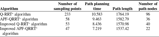
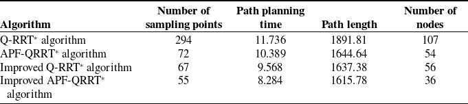
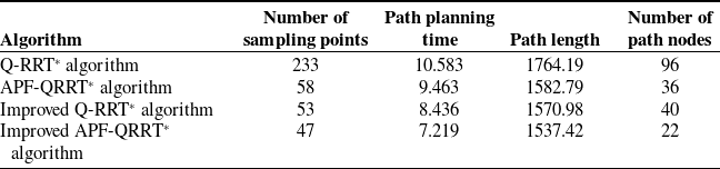
In the simulation experiment, the green part of the simulation map indicates the obstacles, the white part is the feasible space, the pink dot represents the starting point, and the red dot represents the end point. The size of the simulation maps is 1000x1000, the starting point is set to (0, 0), the end point is set to (1000, 1000), the maximum number of iterations are all set to 10,000, and the fixed step size of the traditional Q-RRT* algorithm, the improved Q-RRT* algorithm, APF-QRRT* algorithm, and the improved APF-QRRT* algorithm is set to 20, and the target bias rate is set to 0.3. The sampling times, path planning times, path lengths, and number of path nodes of the traditional Q-RRT* algorithm, the improved Q-RRT* algorithm, the APF-QRRT* algorithm, and the improved APF-QRRT* algorithm are tested in two environments, a small number of obstacles environment and a random multiple obstacles environment. Figure 9 shows the path planning simulation results of the four algorithms in a sparse obstacle environment. Figure 10 shows the path planning simulation results of the four algorithms in a random multi-obstacle environment. To ensure the fairness of the experiments, 20 experiments will be conducted for each of the four algorithms in the same map, and finally, all the experimental results will be summarized and averaged for analysis.
Performance simulation results of the four algorithms under environment 1.
Performance simulation results of the four algorithms under environment 2.

In Table II, it can be seen that in the simple obstacle environment, the improved APF-QRRT* algorithm reduced the path planning time by 31.8%, the path length by 12.9%, the number of path nodes by 77.1%, and the number of sampling points by 96.9% compared to the Q-RRT* algorithm; compared to the APF-QRRT* algorithm, the path planning time decreased by 23.7%, the path length by 2.9%, and the number of sampling points by 19%; compared to the APF-QRRT* algorithm, the number of path nodes is reduced by 38.9%, and the number of sampling points is reduced by 19%; compared with the improved Q-RRT* algorithm, the path planning time is reduced by 14.4%, the path length is reduced by 2.1%, the number of path nodes is reduced by 45%, and the number of sampling points is reduced by 11.3%, which proves the effectiveness of this paper’s improved algorithm for path planning in a small number of obstacle environments.
In Tables III, it can be seen that the improved APF-QRRT* algorithm significantly improves the performance metrics compared to the Q-RRT* algorithm in random multiple obstacle environments, the path planning time is reduced by 29.4%, the path length is reduced by 14.6%, the number of path nodes is reduced by 66.4%, and the number of sampling points is reduced by 81.3%; compared to the APF-QRRT* algorithm, the path planning time is reduced by 20.3%, the path length is reduced by 1.8%, the number of path nodes is reduced by 33.3%, and the number of sampling points is reduced by 23.6%; compared with the improved Q-RRT* algorithm, the path planning time is reduced by 13.4%, the path length is reduced by 1.3%, the number of path nodes is reduced by 35.7%, and the number of sampling points is reduced by 17.9%, which proves that the improved algorithm of this paper has a stronger performance in the random multiple obstacle environments has stronger applicability.
Environment 1 four algorithms path planning result map.

Environment 2 four algorithms path planning result map.

To validate the superiority of the improved APF-RRT* algorithm for AGV path planning in complex dynamic environments, tests were conducted on the values of the attraction coefficient
 $k_{attr}$
and repulsion coefficient
 $k_{rep}$
, which most significantly impact the algorithm’s performance. The results are shown in Figure 11.
As shown in Figure 11(a), when the attraction coefficient is set to 1.0, the algorithm converges most rapidly and achieves the lowest final loss value, reaching a minimum of 0.1. This indicates that this value enables optimal performance in guiding the robot toward the target point. As shown in Figure 11(b), when the repulsive coefficients are 0.1, 0.5, 1.0, and 1.5, respectively, significant differences exist in the rate of decrease and final value of the loss function. When the repulsive coefficient is 0.5, the algorithm converges relatively quickly and achieves the lowest loss value, indicating that this selected value can maintain path validity while avoiding collisions.
Based on this foundation, this study conducted performance comparison experiments. The proposed improved APF-RRT* algorithm was compared with the currently advanced multi-strategy bidirectional RRT* algorithm [Reference Huang, Jiang and Xu19], with results shown in Figure 12.
Parameter value test results.

Performance results testing diagram under complex dynamic environments.

As shown in Figure 12, when obstacle density reaches 36.7%, the obstacle avoidance success rate of the APF-RRT* algorithm drops to only 81.6%. The multi-strategy bidirectional RRT* algorithm achieves 84.1% under high obstacle density conditions, while the improved APF-RRT* algorithm maintains an obstacle avoidance rate of 86.4%, further validating its adaptability and reliability in complex dynamic environments.
5. Multi-AGV real vehicle test system development and testing
5.1. AGV system composition and structure
This research section explores in detail the experimental hardware platform for indoor AGVs. The platform covers a variety of key components, including, but not limited to, the chassis structure of the AGV, the Raspberry Pi as the core control unit, the LIDAR and camera for environment sensing, and the OpenCRP controller that performs precise motion control. In addition, power supply modules are involved as well as other external devices such as voice recognition modules and wireless joystick keyboards. These components work together to realize the high-precision motion control of the AGV through the underlying OpenCRP controller [Reference Chen, Gao, Gao and Guo20]. This hardware configuration not only meets the AGV’s navigation and positioning needs but also provides a solid foundation for the system’s scalability and intelligence, thus ensuring that the AGV is able to adapt to diverse industrial and logistics application scenarios. The specific hardware configuration and layout can be referred to Figure 13.
Block diagram of AGV hardware components.

5.2. Construction of AGV system test platform
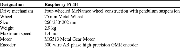
As shown in Figure 14, the host computer used in the establishment of the test platform is an Intel Core i2-11260H processor PC. The AGV is a McNamee Wheel, which has a built-in Raspberry Pi system with an internal wireless network card. Tenda AC100 router is selected. In the whole system, the AGV and the computer are connected through the local area network, and the IP address is set to realize the communication. The specific hardware parameters of the AGV are shown in Table IV.
AGV hardware parameter table.

APF-RRT* algorithm performance data sheet.

Test platforms.

5.3. Pilot test
The single-AGV experiment is the starting point for testing the entire AGV control software system, and it focuses on verifying that the software system performs as expected in terms of path planning. Specifically, the main objective of this experiment is to test whether the system can plan an optimal path for the AGV in a short period of time, as well as a path with fewer turning points. The map of the test field is shown in Figure 15.
Improved APF-RRT* algorithm performance data sheet.

AGV path simulation.

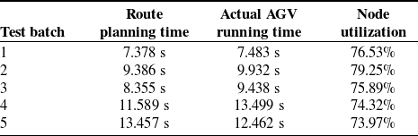
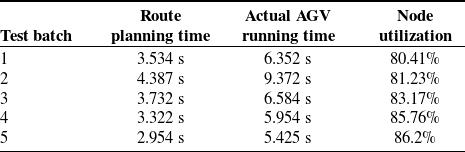
Figure 16 shows the path planned by the APF-RRT* algorithm once, which is transmitted to the AGV through the AGV control system, and the trajectory of the AGV is shown in Figure 17, and the number of its route inflection points is 2. The path planning time, as well as the actual running time of the AGV, is shown in Table V.
APF-RRT* algorithm planning path map.

APF-RRT* algorithm path planning traveling map.

Figure 18 shows the path planned by the improved APF-RRT* algorithm in this paper at one time, which is transmitted to the AGV through the AGV control system, and the trajectory of the AGV is shown in Figure 19, with the number of inflection points of its route being 1. The path planning time as well as the actual running time of the AGV are shown in Table VI.
After five single-AGV test trials, data from Tables V and VI demonstrate that compared to the APF-RRT* algorithm, the improved APF-RRT* algorithm successfully planned the optimal route with the fewest turns and maintained a safe distance from obstacles in all trials. Simultaneously, it achieved a significant improvement in node utilization. The results demonstrate that the improved APF-RRT* algorithm exhibits stable performance and high accuracy in single-AGV path planning, providing a reliable foundation for subsequent system applications and coordinated scheduling of multiple AGVs.
The main purpose of the multi-AGV test is to verify whether the dynamic obstacle avoidance function can be realized when multiple AGVs are in operation, whether the system can detect the occurrence of conflicts, and to determine the driving right of each AGV through the priority level. AGVs with a high level continue to travel, while AGVs with a low level need to stop and wait or re-plan their paths to avoid collisions with other AGVs.
Comparison table of two algorithm characteristics.

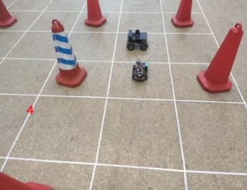
The setup test is shown in Figure 20, setting the AGV1 path from (11,16) to (11,12), setting the AGV2 path from (9,14) to (13,14), and setting the AGV1 priority greater than that of the AGV2. As can be seen in Figure 18, the AGVs will have a conflict at node (11,14). By setting the path through the AGV control system and setting the priority of AGV1 higher than that of AGV2, the trajectories of multiple AGVs and their avoidance process are shown in Figures 21, 22, 23, 24, and 25.
Improved APF-RRT* algorithm for planning path diagrams.

Improved APF-RRT* algorithm path planning traveling map.

Route conflict map.

AGV initial position.

AGV is avoiding dynamic obstacles.

AGV avoidance process.

AGV completes obstacle avoidance.

AGV arrives at target point.

Based on the analysis in Figures 21, 22, 23, 24, and 25, it can be observed that at the conflict point (11,14), AGV1 does not make a stop but continues to follow the planned path. The first AGV2 makes a stop at the neighboring point (10,14) of the conflict point (11,14). AGV2 waits for AGV1 to pass through the conflict area before proceeding. This obstacle avoidance process is as expected and consistent with the simulation results. This shows that the system can effectively handle path conflicts during multi-AGV operation, ensuring the stability and reliability of the system, and verifying the correctness and feasibility of the algorithm.
6. Conclusion
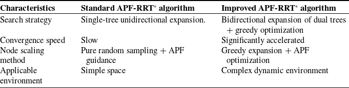
As shown in Table VII, the performance characteristics of the improved APF-RRT* algorithm are compared with those of the standard APF-RRT* algorithm. The comparison results demonstrate that the proposed improved APF-RRT* algorithm exhibits significant advantages in complex dynamic environments.
In this paper, an improved APF-QRRT* algorithm is proposed for mobile robot path planning, taking into account both reachability and safety. Feasible discrete path points are obtained by the Q-RRT* algorithm, the discrete path points are promoted by improving the search strategy of the Q-RRT* algorithm, and the paths are fine-tuned with the help of the APF algorithm to achieve security. The improved APF-QRRT* algorithm theoretically solves the problems of slow convergence speed and redundant nodes of the traditional sampling algorithm. Numerical simulation experiments show that the improved APF-QRRT* algorithm shortens the initial path length and improves the path planning efficiency and security.
Second, this paper completes the construction of the AGV test platform. Through experimental verification, it is shown that the path planning method proposed in this paper can reduce the total operation cost and improve the system operation efficiency. Specifically, the system can quickly and accurately plan the optimal path for each AGV and realize the real-time obstacle avoidance of the trolleys, so as to ensure the smooth execution of the transportation tasks and the efficient operation of the system.
Author contribution
Conceptualization was contributed by W.W., Z.B., and G.C.; methodology was contributed by W.W., Z.B., and G.C.; software was contributed by W.W.; data curation was contributed by Z.B. and G.C.; validation was contributed by Z.B.; formal analysis was contributed by W.W. and Z.B.; investigation was contributed by W.W., Z.B., and G.C.; writing – original draft preparation was contributed by Z.B.; writing – review and editing was contributed by W.W., Z.B., and G.C.; visualization was contributed by G.C.; supervision was contributed by W.W.; project administration was contributed by T.W.; all authors have read and agreed to the published version of the manuscript.
Financial support
This research was funded by the National Natural Science Foundation of China (Grant No. 52105260) as part of the “Hybrid quantitative decoupling research on the in-cylinder mixing performance of gas fuel based on the systematic quantitative evaluation mechanism” project.
Competing interests
The authors declare no conflicts of interest exist.
Ethical approval
Not applicable.