


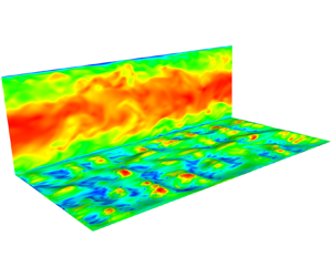



1. Introduction
Studies of turbulent non-Newtonian fluid flow have as many objectives as the nature of the fluids considered and their applications, such as generalized Newtonian (GN) fluids with variable viscosity, power-law (PL) fluids, Casson and Herschel–Bulkley (HB) fluids with a yield stress  $\tau _0$, elastoviscoplastic (EVP) fluids, etc. More than in many other fluid-mechanics problems, direct numerical simulation (DNS) has proven an excellent tool for the exploration of turbulent flow in viscoplastic fluids (Balmforth, Frigaard & Ovarlez Reference Balmforth, Frigaard and Ovarlez2014). The DNS of GN fluids first presented by Rudman & Blackburn (Reference Rudman and Blackburn2006) showed that, in a turbulent pipe flow at a given bulk Reynolds number of 8000, shear thinning reduces the friction factor. In two later contributions of theirs (Singh et al. Reference Singh, Rudman, Blackburn, Chryss, Pullum and Graham2016; Singh, Rudman & Blackburn Reference Singh, Rudman and Blackburn2018), the authors have shown separately the importance of rheology characterization in predicting turbulent pipe flow for these fluids, and the effect of Reynolds number. The DNS study of turbulent PL fluids by Gavrilov & Rudyak (Reference Gavrilov and Rudyak2016) at relatively higher bulk Reynolds number (10 000–20 000) confirmed Reference Singh, Rudman and BlackburnSingh et al.'s results. According to them, shear thinning decreases the turbulent energy transfer from the axial component to others compared with Newtonian fluids. These results validate the general consensus that these fluids significantly enhance anisotropy of the turbulent fluctuations in the near-wall region (Escudier, Nickson & Poole Reference Escudier, Nickson and Poole2009). More recently, Singh, Rudman & Blackburn (Reference Singh, Rudman and Blackburn2017) considered a higher bulk Reynolds number (12 000) that suggested the effect of PL rheology on turbulent pipe flow was mainly significant in the
 $y^+ < 60$ region.
Arosemena, Andersson & Solsvik (Reference Arosemena, Andersson and Solsvik2021) considered GN fluids flowing at a lower bulk Reynolds number. Their statistics revealed that shear-dependent fluid rheology appears to affect the flow within the inner layer and with shear-thinning behaviour; suppressing near-wall structures, thus inhibiting turbulence generating events and leading to different drag reduction features. In a similar investigation, considering now EVP fluids, Izbassarov et al. (Reference Izbassarov, Rosti, Brandt and Tammisola2021) found that the changes in drag are dictated by the Bingham and Weissenberg numbers, depending on the rate of viscoplasticity and elasticity of the fluid. More recently, Karahan, Ranjan & Aidun (Reference Karahan, Ranjan and Aidun2023) performed DNS of GN fluids in a rectangular channel at a relatively low frictional velocity. They observed that the rheology does not play a significant role in the outer layer, and report a strong turbulence anisotropy – as in many previous studies – and larger dissipative structures.
Abdelgawad, Cannon & Rosti (Reference Abdelgawad, Cannon and Rosti2023) showed that the flow in the presence of plastic effects is more intermittent than in a Newtonian fluid, due to the interplay between the classical intermittency of the turbulent dissipation rate and the plastic contribution that instead grows with the Bingham number. Ohta & Miyashita (Reference Ohta and Miyashita2014) performed DNS and large eddy simulations (LES) of wall turbulence of various types of non-Newtonian fluids using a PL type of constitutive laws. They show that the spatial scale of turbulence of these types of fluids can be estimated in the same way as that for Newtonian fluids by normalizing wall turbulence with the locally varying viscosity. Rahgozar & Rival (Reference Rahgozar and Rival2017) studied turbulence decay of a shear-thinning fluid by reference to bulk turbulence in large arteries. Their results not only show modification of the turbulent kinetic energy (TKE) and its dissipation rate, but also indicate significant alteration of the characteristics of the large-scale structures.
The alteration of the turbulent energy cascade by the fluid's plasticity has not known the same interest as in Newtonian fluids. In a thorough study of shear-thinning fluid flow in a pipe, Esmael et al. (Reference Esmael, Nouar, Lefevre and Kabouya2010) showed that a weak chaotic in time and regular in space turbulence prevails in the transitional flow regime. More importantly, the resulting power spectra of the axial velocity fluctuations decay following a two-dimensional turbulence-like power law,  $E \sim k^{-3}$, with
 $k$ being the wavenumber. In their DNS study of a homogeneous isotropic turbulence of an EVP fluid, Abdelgawad et al. (Reference Abdelgawad, Cannon and Rosti2023) addressed the fundamental question as to how the established dissipation theory changes, and how the yield stress affects the energy distribution and balance. Their results showed substantial modifications of the Kolmogorov theory (
 $E \sim k^{-5/3}$ for Newtonian fluids) for Bingham numbers larger than
 $10$, with the emergence of a new scaling law (
 $E \sim k^{-2.3}$), and the dominance of the non-Newtonian flux and dissipation at small and intermediate scales. Thanks to an extensive experimental campaign, Mitishita et al. (Reference Mitishita, MacKenzie, Elfring and Frigaard2021) reported a
 $k^{-7/2}$ scaling in the energy spectra at high wavenumbers for drag-reducing fluid flows compared with the
 $k^{-5/3}$ scaling in the case of water flows. This was attributed either to the decrease in the inertial effect in the presence of polymer solutions, which shrinks the inertial range of scales because of the lower Reynolds numbers, or to the elastic effects that become important at large wavenumbers where the fluid experiences high frequencies.
One of the early attempts to elucidating the role of a complex fluid's rheology on the coherent structures of the underlying turbulence is due to Gampert & Yong (Reference Gampert and Yong1990). The experiment of Peixinho et al. (Reference Peixinho, Nouar, Desaubry and Théron2005) confirmed earlier observations of the flow axisymmetry of yield stress fluids in pipes, which increases with increasing Reynolds number in the transitional regime. In a later paper (Esmael & Nouar Reference Esmael and Nouar2008), a three-dimensional (3-D) description of this asymmetry in transitional flow was demonstrated, accompanied by the characterization of a robust nonlinear coherent structure. Simulation results were then employed by Le Clainche et al. (Reference Le Clainche, Izbassarov, Rosti, Brandt and Tammisola2020), using high-order dynamic mode decomposition, to study the near-wall dynamics, in comparison with Newtonian and viscoelastic fluids. Their work revealed that both elasticity and plasticity have similar effects on the near-wall coherent structures, where the flow is characterized by long streaks disturbed for short periods by localized perturbations. To the best of the authors’ knowledge, the interaction between non-Newtonian fluid flow and wall roughness has never been studied before. For Newtonian fluids, however, the effects of surface roughness in wall-bounded flows has been described thoroughly (Jiménez Reference Jiménez2004; Chung et al. Reference Chung, Hutchins, Schultz and Flack2021) and is not summarized in this introduction. Furthermore, to better position the present study in a practical context, we consider here the case of a rough surface involving small and randomly dispersed elements comparable in size to the inner layer, with  $y^+ < 25$.
In this unprecedented simulation campaign, turbulent flows of Newtonian and non-Newtonian, in particular HB, fluids in smooth and rough channels have been investigated by means of DNS. The focus is on the effect of the non-Newtonian rheology on the flow and its interaction with turbulence and irregular roughness elements; the effect of the particular random roughness type on Newtonian fluid flow is discussed in detail in Narayanan et al. (Reference Narayanan, Nauer, Singh, Belt, Palermo and Lakehal2024). The random roughness with zero skewness chosen here is unique in the sense that it mimics a randomly distorted wall-surface representative of industry-relevant cases, with the relative size of the elements of the order of the inner boundary layer; a differentiating element from most of the previous DNS studies. The results are discussed and compared in a systematic way, from smooth to rough walls, and from Newtonian to non-Newtonian fluids. The effects of shear thinning on the flow are analysed and profiles of turbulence statistics are investigated. In addition, a comparison of the flow structure is presented together with the coherent structures distribution. Finally, energy spectra are compared.
The simulations were carried out using the finite volume computational fluid dynamics (CFD) code TransAT at the TotalEnergies High Performance Computing Center on massively parallel platforms. The simulations were distributed over 1000+ cores. The flow statistics were collected after initial transients for approximately ten flow-through times to ensure that ergodic conditions were attained.
2. Simulation methodology
2.1. Mathematical model
The rough surface is accounted for using a variant of the immersed boundary method of Peskin (Reference Peskin1977) and Mittal & Iaccarino (Reference Mittal and Iaccarino2005), known as the immersed surface technique (IST). Here, the solid object is represented in a Cartesian grid using a solid level set function  $\phi _s(\boldsymbol {x})$; positive values denote the fluid domain, negative values identify the solid domain and the surface of the wall is implicitly represented by
 $\phi _s(\boldsymbol {x})=0$. The fluid domain indicator function
 $H(\boldsymbol {x})$, which has a value of
 $1$ in the fluid and
 $0$ within the solid, varies smoothly as a function of
 $\phi _s(\boldsymbol {x})$, and is given as
 \begin{equation} H(\phi_s) = \frac{1}{2} \left [ 1 + \tanh{ \left ( \frac{2 \phi_s}{\zeta} \right ) } \right ], \end{equation}
where  $\zeta$ is the average mesh size near the fluid–solid surface. The approach, meant to resolve practical flows with complex geometries using a Cartesian mesh, can be used as well to represent segmented roughness elements (Chatzikyriakou et al. Reference Chatzikyriakou, Buongiorno, Caviezel and Lakehal2015) or a continuous rough surface, as in the present study. The discussion of the precise topology of the rough surface used in this study is presented in § 2.3.
The incompressible Navier–Stokes equations are reformulated using the support of the fluid–solid indicator function  $H$. The resulting IST-based mass and momentum conservation equations read
 \begin{gather} \frac{\partial }{\partial x_j} (H u_j)= 0, \end{gather}
 \begin{gather} H\frac{\partial \rho u_i}{\partial t} + \frac{\partial }{\partial x_j} (H \rho u_i u_j) ={-} \frac{\partial p}{\partial x_i} + \frac{\partial }{\partial x_j} ( 2 H \mu S_{ij}) - 2 \mu S_{ij} \frac{\partial H}{\partial x_j}, \end{gather}
where  $\rho$ is the fluid density,
 $\mu$ the viscosity,
 $u_i$ the Cartesian velocity vector and
 $S_{ij}=1/2(u_{i,j}+u_{j,i})$ the strain-rate tensor. In the IST method the no-slip condition at the immersed solid surface is achieved by rewriting the last term in (2.3) as (Beckermann et al. Reference Beckermann, Diepers, Steinbach, Karma and Tong1999)
 \begin{equation} {-}2 \mu S_{ij} \frac{\partial H}{\partial x_j} = \mu \frac{(u_i - u^w_i)}{\zeta} \left | \frac{\partial H}{\partial x_j} \right |, \end{equation}
where  $u^w$ is the wall velocity that is set to zero and
 $| {\partial H}/{\partial x_j} |$ is the surface area density. Note that LES was performed on coarser grids and interpolated on to successively finer grids so as to reach the fully developed turbulent state efficiently.
For the non-Newtonian fluid simulations, the viscosity is prescribed using the HB rheology:
 \begin{equation} \mu = \frac{\tau_0}{\dot{\gamma}} (1 - e^{{-}M \dot{\gamma}}) + K \dot{\gamma}^{(n-1)}, \end{equation}
where  $\dot {\gamma }$ is the magnitude of the rate of strain given as
 $2 \sqrt {S_{ij}\,S_{ij}}$,
 $\tau _0$ is the yield stress,
 $K$ is the consistency index and
 $n$ is the flow index. The above expression includes the Papanastasiou regularization (Mitsoulis & Tsamopoulos Reference Mitsoulis and Tsamopoulos2017) to ensure that the viscosity does not attain unreasonably high values in low strain-rate regions. The constant
 $M$ was set to a value of
 $100$. However, it was noted that due to the fully resolved turbulent fluctuations in all regions of the flow, the regularization was not applied.
2.2. Simulation set-up
Four DNS were performed in this study, namely, Newtonian fluid flow over a smooth wall (NS), Newtonian flow over a rough wall (NR), non-Newtonian flow over a smooth wall (NNS) and non-Newtonian flow over a rough wall (NNR). For all the simulations, the domain consisted of a Cartesian box the size of which was selected to include the largest eddies in the flow and such that the turbulent eddies would not be correlated. Thus, for the smooth-wall flow, the Cartesian box had dimensions  $L_x = 2{\rm \pi} \delta$,
 $L_y = 2\delta$ and
 $L_z ={\rm \pi} \delta$ in the streamwise, spanwise and vertical directions, respectively, where
 $2 \delta$ is the channel height. Since fully developed turbulent channel flow is homogeneous in the streamwise and spanwise directions, periodic boundary conditions were applied in these directions. No-slip boundary conditions were applied both on the upper and lower horizontal planes of the smooth channel. For the rough-wall case, no-slip is enforced by the IST method described earlier.
The flow in the streamwise direction is driven by a constant mean pressure gradient  $\Delta P = \langle -\mathrm {d} p / \mathrm {d}{\kern0.8pt}x \rangle$. The resulting shear Reynolds number is defined as
 $Re_{*} = {\delta u_{*}}/{\nu _w}$, where
 $u_{*} = \sqrt { (\delta /\rho ) \Delta P}$ is the shear velocity and
 $\nu _w$ is the minimum horizontal plane-averaged kinematic viscosity, and variables normalized by
 $u_*$ and
 $\nu _w$ are denoted by the ‘*’ sub or superscript. While in the smooth-wall case the minimum horizontal plane-averaged viscosity is at the wall, in the rough-wall case, it is slightly away from the wall. The
 $Re_*$ for the NNR case is lower than the NNS case due to the higher value of
 $\nu _w$. The wall viscosity for the NNS case was equal to 0.24 Pa s, whereas the lowest viscosity for the NNR case was equal to 0.36 Pa s. For the smooth-wall cases,
 $u_*$ is the same as
 $u_{\tau }$, where
 $u_{\tau } = \sqrt {\tau _w/\rho }$ is the friction velocity and
 $\tau _w$ is the average wall shear stress. Inner scaling is such that the variables are normalized by means of
 $u_\tau$ and
 $\nu _w$, and are denoted by the
 $^+$ superscript or
 $\tau$ subscript. For the rough-wall cases,
 $u_{*}$, in addition to wall shear, also includes the effect of form drag.
The mean pressure gradient was set to  $-5\,{\rm N}\,{\rm m}^{-3}$ for the Newtonian simulations and to
 $-40\,{\rm N}\,{\rm m}^{-3}$ for the non-Newtonian simulations. Due to the nonlinear rheology of non-Newtonian fluids, several iterative simulations with smooth walls were first carried out to estimate the mean pressure gradient that would yield a shear Reynolds number reasonably close to the target value of
 $360$. The final Reynolds numbers achieved for the different cases are presented in table 1.
Reynolds numbers achieved in the simulations.

Turbulent statistics were computed by time averaging the velocity and the pressure fields, once statistically ergodic conditions were obtained. The time-averaged results are further space averaged in the streamwise and spanwise directions throughout the flow domain.
2.3. Surface roughness characterization
Industrial pipes transporting liquid are often hydrodynamically smooth when new; however, over time, the wall surface degrades due to corrosion, erosion and fouling, and its topography becomes irregular with a sand-grain roughness  $r_s$ generally in the range of 30–300
 $\mathrm {\mu }$m. For such sizes at the Reynolds numbers encountered in pipes transporting liquid, the flow is at worst in the transitionally rough regime, i.e. the sand-grain roughness
 $r_s^*$ is generally smaller than 70 wall units. Hence, to get in this study a realistic effect of a randomly distorted wall surface on the turbulent flow, the irregular roughness elements were chosen (i) small enough to satisfy the conditions at which the outer-layer similarity assumption in principle holds, since such conditions also apply to industrial pipes, i.e.
 $\delta / r > 40$, (ii) small enough to stay within the transitionally rough regime (
 $r_s^* < 70$), but at the same time (iii) large enough to observe a reasonable impact on the flow.
In view of that, the roughness was randomly generated with the root-mean-square (r.m.s.) roughness height and spacing between roughness structures as parameters. The standard deviation of the roughness height  $r_{rms}^* = r_{rms} u_*/\nu$ was taken to be
 $7.5$ wall units
 $(\nu /u_*)$ based on
 $Re_{*} = 360$ on each side of the mean surface plane, with the spacing between the structures as
 $100$ wall units. The streamwise and spanwise spacing was chosen to be significantly smaller than the streamwise domain extent of
 $2 {\rm \pi}\delta ^* = 2263$ wall units.
Using these settings, a mesh of  $100$ wall units spacing was created on which random heights were generated with a standard deviation of
 $7.5$ wall units. The rough surface was created by fitting the roughness heights using cubic spline interpolation. This was interpolated onto a sufficiently fine mesh so that the triagulated surface is smooth. This was then exported to a CAD (computer aided design) format supported by the CFD software. Typically, as mentioned in Narayanan et al. (Reference Narayanan, Nauer, Singh, Belt, Palermo and Lakehal2024), organized surface protrusions/obstructions have been considered in the literature. In this case the rough surface consists of both crests and troughs with respect to the mean wall surface at
 $y=0$ and
 $y=2\delta$ of the corresponding smooth-wall simulations. One of the surfaces used in the simulations is presented in figure 1. The maximum crest and trough were found to be
 $23$ wall units with respect to the mean wall surface and the average was found to be
 $5$ wall units.
Surface used for rough channel simulations.

Few references were found addressing similar roughness types, with the closest reference being the work of Busse, Thakkar & Sandham (Reference Busse, Thakkar and Sandham2017) for Newtonian fluids, where the influence of roughness wavenumber filtering on the turbulent profiles is studied for two kinds of surfaces, viz. graphite and grit blasted. Their roughness height distribution is smaller than our work, as shown in figure 2, however, there are notable differences in the surface characteristics. In this study the ratio of the channel half-height to the r.m.s. roughness is  $48$ compared with a highest value of
 $27$ for Busse et al. (Reference Busse, Thakkar and Sandham2017). The roughness height scaled by the outer coordinate is much smaller in the present study. Jiménez (Reference Jiménez2004) states that universal behaviour in the outer layer should be observed for cases where
 $\delta /r > 40$, which is the case here too. More specifically, this similarity hypothesis states that in the outer layer (
 $\delta \ge y \gg \nu /u_{\tau },r$), turbulent quantities normalized by shear velocity scale are independent of the surface condition at sufficiently high Reynolds number, provided that the outer-layer thickness is much greater than the roughness height (
 $\delta \gg r$, see Chung et al. Reference Chung, Hutchins, Schultz and Flack2021).
Comparison of the roughness distribution density function to Busse et al. (Reference Busse, Thakkar and Sandham2017).

Another important difference is that the surface height distributions in Busse et al. (Reference Busse, Thakkar and Sandham2017) had significant skewness (of the two surfaces they studied, one had positive skewness and the other negative), implying that either the crests were higher than the troughs or vice versa. In the current study the surfaces are not skewed (symmetric distribution) as shown in figure 2. Additionally, it appears that our roughness has larger wavelengths (100 wall units) or lower slopes.
2.4. Mesh description
For each DNS, a sequence of LES were performed on successively refined grids for the turbulence to develop quickly on the finer grid. The coarse grid results, on reaching statistical stationarity, were interpolated on to the next finer grid. For the LES, the WALE (wall adapting local eddy-viscosity) subgrid-scale model (Nicoud & Ducros Reference Nicoud and Ducros1999) was used to account for the effect of the unresolved turbulence; the effect of the non-Newtonian rheology on the subgrid model (as discussed in Ohta & Miyashita Reference Ohta and Miyashita2014) was neglected. For the DNS, the subgrid-scale model was switched off and simulations were carried out only with discretized Navier–Stokes equations. Meshes 1 to 4 correspond to increasingly refined LES (table 2 for smooth-wall cases), while mesh 5 is DNS. The size of the DNS grid is consistent with a previous work (Chatzikyriakou et al. Reference Chatzikyriakou, Buongiorno, Caviezel and Lakehal2015, using TransAT and its IST meshing feature for roughness), where it has been shown that the 15 and 26 million-cell runs gave similar results. The advantage of IST in the particular context of hemispherical roughness can be demonstrated by comparing the work of Chatzikyriakou et al. (Reference Chatzikyriakou, Buongiorno, Caviezel and Lakehal2015) to that of Wu, Christensen & Pantano (Reference Wu, Christensen and Pantano2019), the later one using body-fitted spectral elements that required almost nine times more grid cells (normalized by the size of the computational domain) than the first one, even though the two studies used comparable set-ups in terms of roughness distribution and flow conditions.
Mesh used for NS and NNS simulations.

The intermediate and final mesh sizes for the rough-wall cases are detailed in table 3. In the rough-wall case the whole roughness region is refined uniformly, with the mesh size increasing towards the centre only away from the roughness region, thereby requiring a larger number of cells in the wall-normal direction. The presence of the solid object and the IST method means that a few cells are within the solid surface as well. For the normalized mesh intervals, the Newtonian viscous length for  $Re_{\tau } = 360$ is used for both cases.
Mesh used for NR and NNR simulations.

Mesh convergence for the NR case was demonstrated in Narayanan et al. (Reference Narayanan, Nauer, Singh, Belt, Palermo and Lakehal2024) by comparing the mean and streamwise fluctuating velocities for the final three meshes. The lower Reynolds number for the NNR case and the significant reduction in the energy in the higher wavenumbers reported in § 5.6 imply lower resolution requirements for the NNR case as compared with the Newtonian case.
2.5. Fluid properties
The fluid density was specified as  $1000\ {\rm kg}\ {\rm m}^{-3}$ for all the simulations. For the Newtonian cases used for comparison, the viscosity was set to
 $6.944\times 10^{-2}\ {\rm Pa}\ {\rm s}$. For the non-Newtonian fluid, the parameters for the HB law were set as
 $\tau _0 = 2.18\ {\rm Pa}$,
 $K = 1.42\ {\rm Pa}\ {\rm s}^{n}$ and
 $n=0.567$, which are representative of a paraffinic crude oil below the wax appearance temperature (Palermo & Tournis Reference Palermo and Tournis2015). The non-Newtonian behaviour of crude oils below the wax appearance temperature can be explained by the fact that wax crystals aggregate into large porous particles, whose effective volume fraction is larger than the actual volume fraction of the wax crystals due to porosity. The size and the effective volume fraction of the aggregates is a function of the shear stress applied on them, leading to an effective viscosity dependent on the shear rate.
The Bingham number (Bn) for a HB fluid is defined as
 \begin{equation} {Bn} = \frac{\tau_0}{K} \left ( \frac{L}{V} \right )^n, \end{equation}
where  $L$ and
 $V$ are characteristic length and velocity scales, respectively. Using the channel height (
 $2\delta$) and the bulk velocity as the respective scales we obtain
 ${Bn} = 0.83$ for the NNS case. Due to a change in the bulk velocity and wall shear, the Bingham number for the NNR case turns out to be
 $0.95$. Alternatively, the effect of the yield stress can also be characterized as the Bingham number in wall units,
 ${X} = \tau _0/\tau _w$, which gives
 ${X} = 0.11$ for the NNS case and
 $0.135$ for the NNR case.
2.6. Computational algorithm
The simulations were performed with the finite volume CFD code TransAT , which solves (2.2) and (2.3) on a collocated Cartesian grid. The convection terms in the momentum equations are discretized using the third-order QUICK scheme (Leonard Reference Leonard1995) and the diffusion terms by second-order central differences. The higher-order convection schemes are implemented using the deferred correction approach of Rubin & Khosla (Reference Rubin and Khosla1977). The pressure-correction equation is solved using the SIMPLEC pressure-correction method of Van Doormaal & Raithby (Reference Van Doormaal and Raithby1984). The second-order implicit Euler backward time-stepping scheme was used for the time derivative discretization given for one of the velocity components (referred to as
 $u$ in (2.7)) as
 \begin{equation} \left. \frac{{\rm d} u}{{\rm d}t}\right |^{m+1} = \frac{3 u^{m+1} - 4 u^{m} + u^{m-1}}{2 \Delta t}, \end{equation}
where  $\Delta t$ is the time step. The superscripts
 $m+1$,
 $m$ and
 $m-1$ denote the time level being solved and the two previous times, respectively. The time step was adaptive with a Courant number of
 $\approx 0.3$ to guarantee good time accuracy of the simulations.
3. Validation: non-Newtonian fluids
The flow structure in the vicinity of the roughness layer is depicted in figure 3 by the axial velocity normalized to the bulk velocity. For the Newtonian flow case reported in figure 3(a), the behaviour in the roughness region is different from that observed in general for roughness being modelled as structured rows of cubic protrusions, etc. The velocity shows accelerations and recirculations alternating in the troughs, as shown in the zoomed portion of the contour plot. The roughness induces flow separation just downstream of some of the elements, which enhances form-drag contribution of the total drag. For the HB fluid (figure 3b), the flow in the roughness region differs also from the Newtonian fluid result. Again, the velocity shows separation, acceleration and recirculation in the troughs, responsible for the generation of form drag. The fluctuations appear damped in the core flow, as if this were to undergo a process of relaminarisation.
Vertical slice of instantaneous velocity with detail of the wall neighbourhood (zoomed in). (a) NR, (b) NNR.

The non-Newtonian fluid DNS is compared here with equivalent work in the literature. To the best of the authors’ knowledge, simulation data of non-Newtonian fluid flow in rough channels are new and no point of comparison could be found in the published literature. However, our DNS of HB fluid in a smooth channel can be compared with the results from Rudman & Blackburn (Reference Rudman and Blackburn2006). They considered a HB fluid with a yield stress of  $0.1 \tau _w$ and a flow index of
 $n = 0.6$. In the present study the flow index of
 $n=0.567$ is very close and, for the smooth-wall case,
 $\tau _0 = 0.11 \tau _w$ is also very close to their conditions. The Bingham number in their case was
 $0.7$ compared with
 $0.83$ in the present smooth-wall case. Comparison to the data of Rudman & Blackburn (Reference Rudman and Blackburn2006) is presented in figure 4, keeping in mind that their results are for a pipe flow and at a lower frictional Reynolds number (
 $Re_{\tau } = 180$). The mean velocity profiles are close; the slightly higher velocity in the present study is most likely due to a slightly smaller flow index, since the drag reduction increases with a decreasing flow index, at least for PL fluids, according to Singh et al. (Reference Singh, Rudman and Blackburn2017). Although the normal fluctuation profiles do not exactly match the pipe flow near the wall, the match in the outer layer is excellent, thereby instilling confidence in the results obtained in this study.
Profiles for the NNS compared with pipe flow results of Rudman & Blackburn (Reference Rudman and Blackburn2006). (a) Mean velocity profiles, (b) streamwise velocity fluctuations, (c) wall-normal velocity fluctuations, (d) spanwise velocity fluctuations, (e) Reynolds stress profiles.

4. Mean velocity profile for HB fluids
In this section we discuss the mean velocity profile and the structure of the boundary layer through its characteristic parameters in the light of the established wall laws for smooth and rough walls.
4.1. The DNS results for mean streamwise velocity and viscosity
The mean velocity profile for the NNS case is shown in figure 5. The maximum velocity at the channel centre is significantly higher for the non-Newtonian case, which is the sign of drag reduction. As shown in the mean stress balance (see figure 13), the viscous stress remains significant compared with the turbulent stress for the non-Newtonian case. This is due to the fact that as the strain rate decreases away from the wall, the viscosity increases nonlinearly, preventing the viscous stress from decreasing. This means that the mean velocity profile cannot be as flat as in the Newtonian cases, where turbulent mixing dominates immediately beyond the viscous sublayer. The LES results of Zheng et al. (Reference Zheng, Saidoun, Palermo, Mateen and Fogler2017) showed the same behaviour. Fitting a logarithmic law gives the von Kármán  $\kappa = 0.36$ and the intercept
 $B = 8.0$ for the smooth wall.
Comparison of mean streamwise velocity profiles. (a) Newtonian versus non-Newtonian, (b) NNS versus NNR.

The roughness-induced form-drag contribution to the overall drag affects the mean streamwise velocity profile such that the log law can be rewritten as (Durbin et al. Reference Durbin, Medic, Seo, Eaton and Song2001)
 \begin{equation} U^+(y^+) = \frac{1}{\kappa} \ln(y^+) + B + \Delta B_r (r^+), \end{equation}
where  $y^+$ is the non-dimensional distance to the wall. The shift in the mean velocity profile due to roughness is denoted by
 $\Delta B_r$ and depends on the roughness height
 $r^+ = r \,u_{\tau }/\nu _w$. The function
 $\Delta B_r$ for intermediate roughness
 $2.25 \leq r^+ \leq 90$ is given as
 \begin{equation} \left. \begin{gathered} \Delta B_r(r^+) = \xi(r^+) \left [ 8.5 - B - \ln(r^+)/\kappa\right ], \\ \xi(r^+) = \sin \left (\frac{{\rm \pi}/2 \ln(r^+{/}2.25)}{\ln(90/2.25)} \right ), \end{gathered} \right\} \end{equation}
with  $B=5.5$ and
 $8.0$ for Newtonian and non-Newtonian flows in a smooth channel, respectively. For the NNR case, we use the same equation but with the expression for
 $\Delta B_r (r^+)$ modified to take account of the increase in the value of the intercept
 $B$ from
 $5.5$ to
 $8.0$. The value of the constant
 $8.5$ is increased by the same amount to
 $11$ to give
 \begin{equation} \Delta B_r(r^+) = \xi(r^+) \left [ 11.0 - B - \ln(r^+)/\kappa\right ]. \end{equation}
Comparison of the mean velocity profiles for the non-Newtonian cases is presented in figure 5. For calculating  $\Delta B_r$,
 $r^+ = 6.1275$ is used instead of
 $7.5$ based on the
 $Re_*$ being
 $294$ instead of
 $360$ for the Newtonian case. The rough-wall correction matches the DNS results very well with no adjustment to
 $\kappa$ or
 $B$. Based on these results the function
 $\Delta B_r$ can be generalized and written as
 \begin{equation} \Delta B_r(r^+) = \xi(r^+) \left [ 3.0 - \ln(r^+)/\kappa\right ] \end{equation}
to account for both the NR and NNR cases. The bulk velocity is reduced from  $2.94\,\textrm {m}\,\textrm {s}^{-1}$ for the smooth wall to
 $2.33\,\textrm {m}\,\textrm {s}^{-1}$ due the wall roughness (a
 $20\,\%$ decrease). Due to the reduction in the bulk velocity and, therefore, the maximum strain rate, the wall viscosity (in practice, the minimum viscosity near the wall) reaches a value of 0.36 Pa s that is
 $50\,\%$ higher than the smooth-wall viscosity value of 0.24 Pa s.
The variation of the viscosity for the NNS and NNR cases is presented in figure 6, both as original values and normalized values ( $\nu ^+ = \nu /\nu _w$). The viscosity is seen to be similar for both cases when looking at the original values in the outer region. If the viscosity is normalized individually by the respective wall viscosities, the maximum values at the channel centre would appear quite different given the
 $50\,\%$ difference in the wall viscosities. The viscosity at the centre of the channel is somewhat lower for the NNR case indicating higher turbulent activity (since the bulk velocity is lower) in an absolute sense for the imposed pressure gradient of
 $40\,\textrm {Pa}\,\textrm {m}^{-1}$. The near-wall variation of
 $\nu ^+$ is presented in figure 6(b) with respect to
 $y^* = y \,u_*/\nu _w$ using a logarithmic scale. For the NNS case,
 $\nu ^+$ is equal to
 $1$ at the wall and remains constant in the viscous sublayer, where the shear is constant. For the NNR case,
 $\nu ^+$ is equal to
 $1$ at
 $y^* \approx 3\unicode{x2013} 4$, below which viscosity starts to increase in the vicinity of the roughness elements. In the range between
 $4 < y^* < 30$ the variation of the non-dimensional viscosity is similar to the smooth case, after which they deviate in the outer layer due to differences in the bulk velocity.
Variation of viscosity for non-Newtonian flow. (a) Outer scaling. (b) Inner scaling.

The structure of the turbulent boundary layer with regard to satisfying a logarithmic law or a power law can be analysed by plotting the parameters  $\gamma = y^+ \partial U^+/\partial y^+$ and
 $\beta = (y^+/U^+) \partial U^+/\partial y^+$, respectively. Figure 7 shows that for the rough surface, the interval where a log-law behaviour is observed is smaller (also due to the lower
 $Re_*$) with almost the same value of
 $\kappa$. In general, the log-law interval for the non-Newtonian cases is smaller than for the Newtonian cases. The variation of
 $\beta$ shows that for both the smooth and rough non-Newtonian cases, the interval where
 $\beta$ is constant is significantly smaller as compared with the Newtonian case. This is an interesting result and it appears that further work is needed to develop the functional form of the mean velocity profile for non-Newtonian and in particular HB fluids.
Indicators for the analytical form of the mean velocity profile. (a) Diagnostic for log law  $\gamma$. (b) Diagnostic for power law
 $\beta$.

4.2. The DNS results for form drag and friction factor
In this section we present domain-averaged results such as viscous drag, form drag and comparison of friction factors with those obtained using empirical correlations such as those based on the Colebrook–White equation (Menon Reference Menon2014). Before diving into the numbers, qualitative snapshots of the flow are discussed in the context of figure 8, showing the wall shear patterns along with the contours of the streamwise velocity normalized by the bulk velocity  $u_b$.
Instantaneous contours of normalized streamwise velocity and wall friction. Note that the same colour scheme is used for different quantities with vastly different ranges. (a) NNS, (b) NR, (c) NNR.

Figure 8(a) shows the HB fluid case for the smooth wall (NNS), and figure 8(b,c) for the rough wall (NR and NNR). Note that different frictional velocity scales are used in the figures to provide a better appreciation of the simulations and key observations. For the NNS case, streamwise streaks of high and low shear can be observed, with the very peculiar behaviour of continuous, unperturbed streaks occupying the domain length. This differs from the NS case discussed in Narayanan et al. (Reference Narayanan, Nauer, Singh, Belt, Palermo and Lakehal2024), where the streaky structure patterns are more abundant and shorter, and exhibit clearly alternating regions of low- and high-speed fluid.
The case with roughness (NR) suggests that the near-wall streaks are now considerably shortened by the surface crests. The streamwise correlation lengths in the wall region are now smaller and also proportional to the roughness wavelengths. As shown by Ma, Alamé & Mahesh (Reference Ma, Alamé and Mahesh2021), the crests of the undulating wall surface are associated with higher shear stress regions and the troughs/valleys with low-shear stress where reverse flow occurs. The same phenomenon was observed in the DNS of interfacial, sheared air–water flow of Fulgosi et al. (Reference Fulgosi, Lakehal, Banerjee and DeAngelis2003). Furthermore, the coherence of the streaky structures over the rough wall is affected, and the flow establishes in the new patterns sketched by the roughness surface. For the NNR case, the streaky structure observed in the NNS case is broken down by the roughness elements, giving regions of high shear at the crests and low shear at the troughs, although the structure is different from the NR case (as highlighted in § 5.5).
Wall roughness causes an increase in the total drag (viscous and form-drag contributions), resulting in a lower  $Re_{\tau }$ for the same pressure forcing, which also results in a lower bulk (and mean centreline) velocity. The dynamic force balance shown in figure 9 indicates that for the non-Newtonian case, viscous shear at the wall accounts for 81 % of the applied pressure forcing and form drag for 19 % (compared with 25 % for the NR case, see Narayanan et al. Reference Narayanan, Nauer, Singh, Belt, Palermo and Lakehal2024). It appears that the high viscosities in the troughs of the roughness elements and the persistence of viscous shear in the boundary layer reduces the shielding effect of the roughness elements, thereby reducing the form-drag compared with a Newtonian fluid.
Time variation of normalized viscous drag and form drag for the NNR case.

Concerning the averaged quantities, the effect of roughness for the non-Newtonian flow is more significant compared with Newtonian flow. Even though the reduction in the bulk velocity due to roughness is the same for both fluids ( ${\approx }20\,\%$) and the reduction in
 $u_{\tau }$ is higher for the Newtonian case (
 $13\,\%$ vs
 $9\,\%$), the reduction in
 $Re_{\tau }$ is
 $33\,\%$ for the non-Newtonian case compared with
 $13\,\%$ for the Newtonian. This large change in the
 $Re_{\tau }$ is due to the increase in the wall viscosity.
One of the increasingly validated hypotheses in rough-wall turbulence is the one proposed by Napoli, Armenio & De Marchis (Reference Napoli, Armenio and De Marchis2008), which relates the ratio of the form drag to the total drag to the effective slope of the rough surface. In Narayanan et al. (Reference Narayanan, Nauer, Singh, Belt, Palermo and Lakehal2024) it was shown that the present NR data are in very good agreement with the data of Napoli et al. (Reference Napoli, Armenio and De Marchis2008), thus confirming the hypothesis of a universal behaviour of rough walls for Newtonian fluids. However, the data for the HB fluid (figure 10) diverges slightly from that of Napoli et al. (Reference Napoli, Armenio and De Marchis2008) due to the fact that the form drag is lower than in the Newtonian case at 19 % of the total drag, while the effective slope is the same in both cases. The data suggest that this hypothesis may not hold for non-Newtonian flows, thereby motivating further studies for different values of effective slope and differing rheologies.
Comparison of the form-drag coefficient versus the effective slope with data from Napoli et al. (Reference Napoli, Armenio and De Marchis2008).

In order to estimate the friction coefficient for non-Newtonian fluids using the Colebrook–White correlation, a definition of the Reynolds number is required. This is not straightforward since the viscosity varies from low values near the wall to significantly higher values at the channel centre. Metzner & Reed (Reference Metzner and Reed1955) derived a generalized Reynolds number for PL fluids such that the laminar flow friction coefficient of  $64/Re_b$ is satisfied also for such fluids. Madlener, Frey & Ciezki (Reference Madlener, Frey and Ciezki2009) extended their work to derive a generalized Reynolds number for HB fluids (
 $Re_{{gen,HB}}$) satisfying the laminar flow friction coefficient for Newtonian fluids given as
 \begin{equation} Re_{{gen,HB}} = \frac{\rho u_b^{n-1} D^n}{(\tau_0/8)(D/u_b)^n + K ((3m+1)/(4m))^n\, 8^{n-1}}, \end{equation}
where
 \begin{equation} m = \frac{n K (8 u_b/D)^n}{\tau_0 + K (8 u_b/D)^n}. \end{equation}
This definition recovers the generalized Reynolds number for PL fluids given by Metzner & Reed (Reference Metzner and Reed1955) when  $\tau _0 = 0$.
The wall friction in channels and pipes can be estimated using the phenomenological Colebrook–White equation (Menon Reference Menon2014) for the Darcy–Weisbach friction factor (  $f$) given as
 \begin{equation} \frac{1}{\sqrt{f}} ={-}2 \log_{10} \left ( \frac{r/D}{3.7} + \frac{2.51}{{Re} \sqrt{f}} \right ), \end{equation}
where  ${Re}$ is the bulk Reynolds number (
 $=\rho u_b D/\mu$) and
 $D$ is the hydraulic diameter of the conduit. The friction factors were computed using the above defined generalized Reynolds number (4.5) and the Reynolds number based on the wall viscosity given as
 \begin{equation} Re_w = \frac{\rho u_b D_h}{\mu_w}, \end{equation}
where  $\mu _w$ is the minimum dynamic viscosity at or near the wall and
 $D_h = 4 \delta$ is the hydraulic diameter for a channel flow. The nominal viscosity at the wall can be calculated as
 \begin{equation} \mu_w = \frac{\tau_0}{\dot{\gamma}_w} + K \dot{\gamma}_w^{n-1}, \end{equation}
where the strain rate at the wall is calculated as
 \begin{equation} \dot{\gamma}_w = \left [ \frac{(\tau_w - \tau_0)}{K} \right ]^{1/n}. \end{equation}
It is noted that the Reynolds number based on the wall viscosity  $Re_w$ has been preferred in the more recent analyses of experimental data (among others Pinho & Whitelaw Reference Pinho and Whitelaw1990; Peixinho et al. Reference Peixinho, Nouar, Desaubry and Théron2005; Escudier et al. Reference Escudier, Nickson and Poole2009; Esmael & Nouar Reference Esmael and Nouar2008) as well as simulation data (e.g. Singh et al. Reference Singh, Rudman and Blackburn2017).
Since the flow is driven by an imposed pressure gradient of  $40\,\textrm {Pa}\,\textrm {m}^{-1}$, the wall shear is 20 Pa for the smooth-wall case, giving a nominal wall viscosity of 0.228 Pa s. In order to find the bulk Reynolds number, an iterative method is used starting with a guess and calculating the friction factor with the guessed value using the Colebrook–White correlation. The friction factor is used to get the wall shear, wall viscosity and bulk velocity until convergence. The wall shear (without form drag) is estimated using the Colebrook–White equation with the same bulk Reynolds number, but with zero roughness. The values obtained using the Colebrook–White correlation for the Reynolds number based on the nominal wall viscosity is compared with the DNS results in table 4.
Comparison between DNS and Colebrook–White predictions using  $Re_w$.

The  $Re_{\tau }$ values for the NNS case do not match because the viscosity at the wall obtained from the DNS (0.24 Pa s) is higher than the nominal value obtained using (4.9) (0.228 Pa s). The nominal viscosity
 $\mu _w$ is not the same as the mean wall viscosity
 $\bar {\mu }_w$ obtained from DNS by time and space averaging, due to the nonlinear dependence between viscosity and strain rate (Singh et al. Reference Singh, Rudman and Blackburn2018). The mean wall viscosity
 $\bar {\mu }_w$ was reported to be
 $2\,\%$ higher by these authors; in the NNS case,
 $\bar {\mu }_w$ is higher than the nominal value by
 $5\,\%$. The bulk velocity predicted by the Colebrook–White correlation is lower than the DNS, however reasonably accurate to within
 $15\,\%$. The bulk Reynolds number is accurate to within
 $10\,\%$ because the lower bulk velocity prediction is compensated by a lower value for the wall viscosity.
For the NNR case, the predicted  $u_{\tau }$ is within
 $2\,\%$ and the bulk velocity is within
 $10\,\%$ of the DNS result. However, the nominal viscosity at the wall is lower by
 $18\,\%$ compared with the DNS; 0.293 Pa s as compared with 0.36 Pa s. Estimating the wall viscosity accurately is very important to obtain an accurate estimate of the pressure drop. The difference could be potentially associated with the skewness in the velocity fluctuation distribution function and appears to be an interesting avenue for further research. The wall shear is predicted to be 78 %, giving a form-drag component that is 22 %, which is a movement in the direction of the 81-19 % split given by the DNS. Overall, the use of
 $Re_w$ as the input to the Colebrook–White equation seems to give a reasonable estimate for non-Newtonian flows, although improvements may be possible.
The use of  $Re_{{gen,HB}}$ for the turbulent flow regime to predict the friction factor using the Colebrook–White equation did not give accurate results. The comparison to DNS is presented in table 5. Note that
 $Re_{\tau }$ is not presented in this case due to uncertainty in its definition. The predicted values for
 $Re_b$ show that
 $Re_{{gen,HB}}$ is not the correct Reynolds number for using the Colebrook–White equation to predict the friction factor for turbulent non-Newtonian flows.
Comparison between DNS and Colebrook–White predictions using  $Re_{{gen,HB}}$.

5. Turbulence statistics
5.1. Turbulent stress profiles
The normal and shear turbulent stresses are compared in figure 11 for the NS and NNS simulations. The notable observation is the significant increase in the streamwise velocity fluctuations across the channel at the expense of a similar reduction in the spanwise and vertical velocity fluctuations  $\overline {v'^2}$ and
 $\overline {w'^2}$. This matches the results presented by Singh et al. (Reference Singh, Rudman and Blackburn2017) for PL fluids, where they suggest that the reason is a decreased energy transfer from axial velocity fluctuations to transverse components via pressure fluctuations. The variation of the turbulent shear stress
 $\overline {u'v'}$ with inner scaling is presented in figure 11(d). A marked reduction in the turbulent shear stress is observed compared with Newtonian fluid flow, signifying an overall reduction in turbulence intensity.
Comparison of turbulent stresses between Newtonian and non-Newtonian fluid flows, for the smooth-wall case. (a) Streamwise velocity fluctuations. (b) Wall-normal velocity fluctuations. (c) Spanwise velocity fluctuations. (d) Reynolds stress.

Comparison of turbulent stresses between NNS and NNR cases is presented in figure 12; wherein the values normalized by both  $u_{\tau }$ and
 $u_*$ are presented. The influence of roughness on the turbulent fluctuations for non-Newtonian flow is the same as for Newtonian flow in the sense that there is a significant enhancement of the turbulence stresses in the roughness sublayer, in particular for the turbulent Reynolds shear stress (bottom right). Additionally, as observed for the Newtonian case (Narayanan et al. Reference Narayanan, Nauer, Singh, Belt, Palermo and Lakehal2024), the peak value of the streamwise turbulent normal stress is significantly lower than for the smooth-wall case, whereas the transverse components do not show any decrease. It appears that for the roughness height studied, similar to Newtonian fluids, the effect of roughness is not felt in the outer region and a good overlap is observed when scaled with
 $u_*$, even though the
 $Re_*$ values are different for the two non-Newtonian cases due to the difference in the reference near-wall viscosities. Therefore, for a given driving force (pressure gradient), increased turbulence production and intensity is restricted to the inner region. It also shows that the wall roughness does not change the nature of non-Newtonian turbulence, which is different from Newtonian turbulence, in particular, the significance of the mean viscous stress all along the boundary layer (see § 5.2).
Comparison of turbulent stresses between NNS and NNR cases. (a) Streamwise velocity fluctuations. (b) Vertical velocity fluctuations. (c) Spanwise velocity fluctuations. (d) Reynolds stress.

5.2. Mean momentum balance
The mean (time and space-averaged) streamwise momentum equation for a channel flow shows that the mean streamwise pressure gradient is balanced by a cross-stream stress gradient. The sequential averaging referred to as the double-averaging decomposition of the velocity field (Yuan & Aghaei Jouybari Reference Yuan and Aghaei Jouybari2018; Ma et al. Reference Ma, Alamé and Mahesh2021) shows that roughness introduces a dispersive stress in the vicinity of the roughness elements, coming from the spatial variation of the time-averaged quantities. Roughness also adds a pressure drag force to the mean streamwise momentum balance. In order to retrieve the classical form of the balance for smooth walls (which is the way to go for Reynolds-averaged Navier–Stokes type of modelling), it is convenient to combine the pressure drag and the dispersive stress to rewrite them as a single shear stress induced by roughness,  $\tau ^r$, which can be simply calculated for Newtonian fluids as (Yuan & Piomelli Reference Yuan and Piomelli2014; Narayanan et al. Reference Narayanan, Nauer, Singh, Belt, Palermo and Lakehal2024)
 \begin{equation} \tau^r = \left\langle - \frac{\mathrm{d} p}{\mathrm{d}{\kern0.8pt}x} \right\rangle \delta \left( 1 - \frac{y}{\delta} \right) - \tau^{\mu} - \tau^{uv}, \end{equation}
where  $\tau ^{uv}$ is the Reynolds shear stress and
 $\tau ^{\mu }$ the viscous shear stress. For a non-Newtonian fluid, an additional shear stress,
 $\tau ^{vv}=2\overline {\nu ' s_{ij}}$, is present due to fluctuations in the viscosity (Singh et al. Reference Singh, Rudman and Blackburn2017). Thus, for a HB fluid in a rough channel, the total stress can be decomposed into
 \begin{equation} \tau = \tau^{uv} + \tau^{\mu} + \tau^{vv} + \tau^r. \end{equation}
The  $\tau ^r$ in this case includes an additional dispersive stress arising out of the viscosity fluctuations.
The mean stress balance for the NNS and NNR cases is presented in figure 13. The key observation in the mean stress balance for non-Newtonian fluids is that the viscous stress  $\tau ^{\mu }$ always remains significant compared with the Reynolds shear stress
 $\tau ^{uv}$, independent of the surface conditions. This is due to the fact that as the strain reduces away from the wall, the viscosity increases nonlinearly, thereby resulting in a significant value for the mean viscous stress over most of the boundary layer. This particular effect has a significant impact on many of the differences between Newtonian and non-Newtonian turbulent flows. Here
 $\tau ^{vv}$ is found to be non-negligible all along the wall-normal direction, accounting for
 $10\,\%$ of the total stress.
Mean shear stress balances for non-Newtonian fluid. (a) NNS, (b) NNR.

For the rough case, it is first noted that the shear stress induced by roughness,  $\tau ^r$, is equal to
 $0.19$ at the wall, in agreement with the contribution of form drag to the total pressure forcing; see figures 9 and 10. This means that the dispersive stress is not significant for the roughness topography studied, corroborating the study of Yuan & Aghaei Jouybari (Reference Yuan and Aghaei Jouybari2018) and Ma et al. (Reference Ma, Alamé and Mahesh2021) where, for a surface with low skewness, the dispersive stress was negligible. The dispersive stress was however significant for the surface in Yuan & Aghaei Jouybari (Reference Yuan and Aghaei Jouybari2018) with large positive skewness and high effective slope. The main difference with the NNS case is the finite value of the turbulent stress at
 $y=0$ that is counterbalanced by the variable viscosity term. The variable viscosity term is not impacted by the rough surface over the entire channel section. The viscous shear stress and the variable viscosity term start to decrease toward zero approximately when the total stress magnitude is close to the yield stress. However, the velocity profile does not become entirely flat, i.e. no formation of a plug in the centre of the channel, because the velocity fluctuations are large enough to exceed the yield stress.
5.3. Stress anisotropy
As can be already guessed from the turbulent normal stress profiles, the anisotropy is sharply increased in the non-Newtonian HB flow studied here. The degree of anisotropy can be evaluated by the ratio of the individual cross-stream turbulent stress components to the streamwise component, as shown in figure 14 comparing NS and NNS cases, as well as the smooth- and rough-wall cases for non-Newtonian flow. Focusing on the channel centre, the ratios of the cross-stream to the streamwise ratios decrease from  $\approx 0.7$ for the Newtonian case to
 $\approx 0.35$ for the non-Newtonian case. The anisotropy in the free-stream turbulence is virtually doubled for the HB fluid. Near the wall, the anisotropy reaches much higher ratios. As in the case of Newtonian flow, the free-stream anisotropy is unaffected by the roughness, as expected by the roughness height
 $\delta /r > 40$. Near the wall, there is a slight reduction in anisotropy due to the enhancement of cross-stream stress components at the expense of the streamwise component. However, the overall effect is a strong increase in anisotropy of turbulence in a HB fluid.
Comparison of turbulence anisotropy. (a) NS and NNS, (b) NNS and NNR.

5.4. Mean TKE budget
The mean TKE equation for general Reynolds averaged, non-Newtonian fluid flows is described as follows:
 \begin{align} \frac{\partial k}{\partial t} + \bar{u}_j\frac{\partial k}{\partial x_j} &={-}\underbrace{\overline{u'_i u'_j} \frac{\partial \bar{u}_i}{\partial x_j}}_{P} -\underbrace{\frac{\partial \overline{u'_i u'_i u'_j}}{\partial x_j} }_{T} - \underbrace{\frac{1}{\rho} \frac{\partial \overline{p'u'_i}}{\partial x_i}}_{\varPi} \nonumber\\ &\quad + \underbrace{\frac{\partial }{\partial x_j} \left (2 \bar{\nu}\, \overline{u'_i s_{ij}} \right )}_{D} - \underbrace{2 \bar{\nu} \,\overline{s_{ij} \frac{\partial u'_i}{\partial x_j}}}_{\varepsilon} \nonumber\\ &\quad + \underbrace{\frac{\partial }{\partial x_j} \left (2 \overline{u'_i \nu'} \,\bar{S}_{ij} \right )}_{\xi_{vv}} - \underbrace{2 \overline{\nu' \frac{\partial u'_i}{\partial x_j}} \,\bar{S}_{ij}}_{\chi_{vv}} \nonumber\\ &\quad + \underbrace{\frac{\partial }{\partial x_j} \left (2\, \overline{\nu' u'_i s_{ij}} \right )}_{\mathcal{D}_{vv}} - \underbrace{2\, \overline{\nu' s_{ij} \frac{\partial u'_i}{\partial x_j}}}_{\varepsilon_{vv}}. \end{align}
The terms in (5.3) are annotated as follows: turbulence production  $P$, turbulent transport
 $T$, pressure diffusion
 $\varPi$, mean viscous diffusion
 $D$ and mean viscous dissipation
 $\varepsilon$. In these quantities,
 $S_{ij}$ and
 $s_{ij}$ denote the mean and fluctuating rate-of-strain tensors, respectively. The four additional terms resulting from the non-Newtonian rheology have been annotated as in Singh et al. (Reference Singh, Rudman and Blackburn2017), and are named as follows (where the subscript
 $vv$ denotes variable viscosity):
 $\xi _{vv}$, mean shear turbulent viscous transport;
 $\chi _{vv}$, mean shear turbulent viscous dissipation;
 $\mathcal {D}_{vv}$, viscous turbulent transport; and
 $\varepsilon _{vv}$, turbulent viscous dissipation.
For rough-wall flows, when resorting again to the sequential double-averaging decomposition, two additional production terms induced by the dispersive shear, denoted as  $P_m$ and
 $P_w$ (Yuan & Aghaei Jouybari Reference Yuan and Aghaei Jouybari2018), add to
 $P$, besides the turbulent transport term due to wake fluctuations (
 $T_w$), and the viscous (
 $D_r$) and pressure diffusion (
 $\varPi _r$) terms associated with form drag.
Firstly, the variable viscosity terms  $vv$ are presented in figure 15. It is clear that the terms arising due to non-Newtonian rheology are significant contributors to the TKE balance. In particular,
 $\xi _{vv}$ and
 $\chi _{vv}$ are very consequential in the viscous sublayer and
 $\varepsilon _{vv}$ gains in magnitude towards the outer layer. Additionally, the sum of all the terms (not shown here) remains as significant as the largest terms. Singh et al. (Reference Singh, Rudman and Blackburn2017) classify (as evidenced by the names)
 $\chi _{vv}$ and
 $\varepsilon _{vv}$ as dissipation terms, thereby defining a total dissipation
 $\varepsilon _T = \varepsilon + \chi _{vv} + \varepsilon _{vv}$ and
 $\xi _{vv}$ and
 $D_{vv}$ as diffusive transport terms contributing to a total diffusion
 $D_T = D + D_{vv} + \xi _{vv}$. It is noteworthy that both
 $\varepsilon _{vv}$ and
 $\chi _{vv}$ are positive as shown by Singh et al. (Reference Singh, Rudman and Blackburn2017) for shear-thinning fluids and they change sign for shear-thickening fluids based on the expected correlation between the viscosity and the strain rate. Here
 $\xi _{vv}$ and
 $D_{vv}$ change signs several times exhibiting behaviour similar to the Newtonian transport terms such as
 $T$,
 $\varPi$ and
 $D$. One of the questions that arises is the classification of
 $\chi _{vv}$ as dissipation, especially given the interaction of the turbulent viscosity, velocity gradient correlation with the mean strain rate. In the rough-wall case a significant increase in
 $\varepsilon _{vv}$ is observed along with a movement of the peak dissipation towards the wall. In general the movement towards the wall is observed for all quantities, as also observed for the Newtonian case.
Non-Newtonian (variable viscosity) terms in the TKE balance. (a) Smooth wall. (b) Rough wall.

The TKE budgets for NS and NNS (with  $D_T$ and
 $\varepsilon _T$ as defined above) are shown in figure 16(a,b). The qualitative behaviour of the TKE budget for the non-Newtonian case is very similar to the Newtonian case, except that all the quantities have lower values. Turbulence production, in particular, is significantly lower in the non-Newtonian case. This is directly related to the significant reduction in the turbulent stress
 $\overline {u'v'}$ for the non-Newtonian case as shown in figure 11. The balance in the viscous sublayer is between viscous dissipation and turbulent diffusion, as is well known for Newtonian flow. Figure 16(c) shows the balance when
 $\chi _{vv}$ is counted as a production term and added to
 $P$ such that
 $P_T = P + \chi _{vv}$ and
 $\varepsilon _T = \varepsilon + \varepsilon _{vv}$. In this interpretation, the mean viscous dissipation increases back to levels in the Newtonian flow, and the peak production also increases, although still significantly lower than in the Newtonian flow. However, turbulence production does not go to zero in the viscous sublayer (due to
 $\chi _{vv}$) but instead reaches a constant value at the wall. The balance in the viscous sublayer is between viscous dissipation on one hand and production and diffusion on the other.
Turbulent kinetic energy balance. (a) NS, (b) NNS, (c) NNS –  $\chi _{vv}$ as production, (d) NNR.

For smooth walls, the main balance in the viscous sublayer is between mean viscous diffusion and dissipation with turbulence production going to zero rapidly as the wall is approached. For rough walls, turbulent dissipation balances the sum of turbulence production and mean viscous diffusion. In short, the effect of roughness on turbulence is to a large extent independent of the fluid rheology.
The pressure transport term  $\varPi$ is known to redistribute energy from the streamwise component to the cross-stream components, inclining to make the flow isotropic. The term is therefore also called the return-to-isotropy term. Based on the discussion in the preceding section on stress anisotropy, the pressure diffusion term is expected to be significantly smaller for the non-Newtonian flow. The comparison of the pressure diffusion term presented in figure 17 shows, as expected, a reduction by a factor of three, thereby pointing towards increased anisotropy in the turbulent normal stresses.
Comparison of the pressure diffusion term between Newtonian and non-Newtonian flow.

The ratio of turbulence production to dissipation is presented for all the four cases in figure 18. As noted earlier for Newtonian flow, the  $P/\varepsilon$ ratio for the rough wall matches with the smooth-wall case in the outer layer even for the non-Newtonian flow. The profile for non-Newtonian flow is, however, very different from Newtonian flow. Firstly, the peak value near the wall is significantly lower for non-Newtonian flow. Additionally, the ratio continuously reduces in the outer layer in contrast to Newtonian flow where there is a second maximum at
 $y/\delta \approx 0.4$. At
 $y/\delta = 0.6$ the ratio for the Newtonian case is five times larger than the non-Newtonian flow. This is an important parameter in averaged turbulence modelling and will definitely serve as an important behaviour to capture correctly in such models. Figure 18(b) compares the ratio
 $P/\varepsilon$ to
 $P/\varepsilon _T$ and
 $(P+\chi _{vv})/(\varepsilon + \varepsilon _{vv})$. In this case, the ratio is enhanced in the outer layer, however, it is still quite different from the Newtonian profile. It is noteworthy that adding
 $\chi _{vv}$ to
 $P$ and removing from
 $\varepsilon _T$ does not change the ratio significantly.
Ratio of turbulence production to mean viscous dissipation. (a) All cases, (b) NNS case comparison to  $P/\varepsilon _T$ and
 $(P+\chi _{vv})/(\varepsilon + \varepsilon _{vv})$.

5.5. Flow structures
In Newtonian wall-bounded flow, turbulence is sustained by the continuous process of growth and breakdown of streamwise elongated structures. Momentum is extracted from the outer region to the inner region and final dissipation into heat as an effect of the viscous forces. In particular, streamwise velocity streaks are generated by streamwise vortices. Figure 19 compares the  $u$-velocity contours of the Newtonian and HB fluid fields at various near-wall horizontal planes; here we only consider the case of a smooth channel. Figure 19(a,c,e,g,i) shows the footprint of the streamwise vortices usually observed in the turbulence of Newtonian fluid flows, with negative streaks weakening away from the wall. The non-Newtonian fluid flow results (right column) show however a peculiar persistence of these low-speed streaks, along the entire domain, the trace of which suggest larger structures than in Newtonian fluid turbulence. This is mainly due to the significantly lower energy in the smaller scales, whereby the structures appear unbroken and persistent. A similar behaviour was observed by Anbarlooei et al. (Reference Anbarlooei, Cruz, Ramos, Santos and Silva Freire2018).
Instantaneous axial flow velocity in the smooth channel at different heights for Newtonian and non-Newtonian fluids. (a) Newtonian  $y^+ = 5$, (b) non-Newtonian
 $y^+ = 5$, (c) Newtonian
 $y^+ = 10$, (d) non-Newtonian
 $y^+ = 10$, (e) Newtonian
 $y^+ = 20$, ( f) non-Newtonian
 $y^+ = 20$, (g) non-Newtonian
 $y^+ = 30$, (h) non-Newtonian
 $y^+ = 30$, (i) non-Newtonian
 $y^+ = 50$, ( j) non-Newtonian
 $y^+ = 50$.

The negative low-speed streaks seem to persist – aligned but not interacting – up to  $y^+=30$ (and probably
 $y^+=40$ too); positive ones have the tendency to rather dilute or better said, increase in size as was reported by Le Clainche et al. (Reference Le Clainche, Izbassarov, Rosti, Brandt and Tammisola2020). At
 $y^+=50$, the streaks start to dislocate and diffuse, in contrast to the Newtonian case, where no change is to be noticed. The enhancement of the streamwise momentum in high-speed streaks in the
 $y^+< 30$ region should corroborate with the reduction of TKE by viscous dissipation as shown in (5.3), and as also shown by Dubief et al. (Reference Dubief, White, Rerrapon, Shaqfeh, Moin and Lele2004). In addition, this points to more energy being contained in the larger spanwise wavelengths compared with Newtonian flow and also an increase in the viscous layer thickness as discussed earlier. The differences in the spanwise energy spectra are discussed in the following section. Additionally the long unbroken streaks also point to higher correlation along the streamwise direction.
Figure 20 comparing the streamwise velocity contours in the rough channel shows another picture. As before, the contours are plotted at five planes:  $y^+= 5, 10, 20, 30$ and
 $50$. Interestingly, until the farthest plane from the wall
 $y^+=50$, the roughness elements seem incapable of breaking the increased correlation in the structures for the HB fluid, as compared with the Newtonian one. The structures seem to persist along the domain as in the smooth surface discussed earlier; the negative structures being more slender than the positive ones. As a consequence, one might expect less form drag being generated, as evidenced by the little impact of roughness on the mean velocity (minimal shift in the outer layer) and shear stress profiles discussed earlier, compared with Newtonian fluid. A close inspection might reveal though that the roughness elements cause the flow to be diverted in either the positive of negative spanwise direction, which should increase the vertical and spanwise fluctuations in the inner layer.
Instantaneous axial flow velocity in the rough channel at different heights for Newtonian and non-Newtonian fluids. (a) Newtonian  $y^+ = 5$, (b) non-Newtonian
 $y^+ = 5$, (c) Newtonian
 $y^+ = 10$, (d) non-Newtonian
 $y^+ = 10$, (e) Newtonian
 $y^+ = 20$, ( f) non-Newtonian
 $y^+ = 20$, (g) Newtonian
 $y^+ = 30$, (h) non-Newtonian
 $y^+ = 30$, (i) Newtonian
 $y^+ = 50$, ( j) non-Newtonian
 $y^+ = 50$.

5.5.1. Coherent structures
To consolidate the findings about the flow structures discussed previously, this section provides additional results showing the coherent structures near the walls for the different simulations performed. Due to the differences in bulk velocity, shear Reynolds number or viscosity between the simulations, a quantitative analysis is difficult, nonetheless qualitative observations can be made. Here, we rely on the so-called Q-vortex identification criterion (Hunt, Wray & Moin Reference Hunt, Wray and Moin1988), a well-known measure of the balance between the rate-of-rotation tensor  $r_{ij}$ and the rate-of-strain tensor
 $s_{ij}$ within the superimposed fluctuating field, and is defined as
 $Q = 1/2(r_{ij}r_{ij} - s_{ij} s_{ij})$; the positive values of which indicate regions where the strength of the rotation overcomes the strain. For this purpose, the probability density functions (p.d.f.) of the identifier were determined and the isosurface thresholds of p.d.f.
 $0.005$ were selected.
Three-dimensional views of the vortex identification criterion are depicted in figure 21 for the four cases studied. The instantaneous isocontours (taken at a randomly selected frame) of  $Q_{\textit {pdf}=0.005}$ coloured by
 $y^+$ show the nature of the structures and their concentration in the boundary layer. Note that the maximum
 $y^+$ used to colour the p.d.f. is rather low (150). Taking the smooth-wall context, the Newtonian fluid flow reveals a rather dense population of small-scale vortices surrounded by hairpin-like structures. In contrast, in the non-Newtonian case, only the large structures can be detected, regardless of the wall surface. It is as if most of the high-frequency motions vanish. Looking now at the NR case confirms the observation made earlier, that is, in the roughness layer the vortical structures are broken and disrupted by the roughness elements. Furthermore, the structures do not seem to rise towards the outer layer as in the case of large surface asperities. Likewise, the interaction between the flow and the roughness elements is not so obvious, although the lift of the flow due to their blockage effect is perceivable. These results raise the following instructive findings: (i) surface roughness generates a denser population of coherent structures, confined mostly in the affected layer
 $y^+<25$, than in the smooth case; and (ii) the hypothetical penetration of these structures to the outer layer is not evidenced. On the contrary, it rather seems that the outer layer has way less structures than the smooth case, which corroborates with the observation concerning
 $S^*$, made in the context of figure 16. In the NNR case the same observation as in the smooth case holds, that is, most of the small-scale structures seem to be smoothed out; the pertinent large-scale ones are somewhat disrupted in the roughness sublayer, but less than in the Newtonian case.
Contour of the Q-criterion with  $\textrm {p.d.f.} = 0.005$, with
 $y+_{max} = 150$. (a) NS, (b) NNS, (c) NR, (d) NNR.

5.6. Energy spectra
The power spectra of the streamwise and the spanwise velocities along the streamwise direction at two locations (  $y/\delta = 0.12$ and
 $1$) are presented in figure 22. Mitishita et al. (Reference Mitishita, MacKenzie, Elfring and Frigaard2021), in their experiments with an aqueous solution of a polymer additive called Carbopol, observe a
 $k^{-7/2}$ scaling of the energy spectrum at larger wavenumbers. They remark that the scaling of energy for higher wavenumbers (
 $k \delta > 5$) is close to
 $k^{-7/2}$ instead of the usual
 $k^{-5/3}$ for the inertial range in Newtonian fluids, indicating a larger power decay for higher wavenumbers (small scales). Therefore, both the
 $-5/3$ and the
 $-7/2$ slopes are shown in the figures for comparison. The spectra are normalized by
 $u_{\tau }^2$. The spectra of the wall-normal velocity is very similar to the spanwise velocity and are therefore not presented here. The spectra for the non-Newtonian cases also show that the simulations are well resolved with a steep drop in the energy towards the highest wavenumbers.
Power spectra in the streamwise  $x$ direction. (a) Streamwise velocity, NS vs NNS. (b) Spanwise velocity, NS vs NNS. (c) Streamwise velocity, NNS vs NNR. (d) Spanwise velocity, NNS vs NNR.

Comparing the power spectra of the Newtonian with the non-Newtonian fluid (figure 22a), it is observed that the energy is concentrated significantly more in the lower wavenumber range both near the wall and at the channel centre. This becomes clearer if one shifts the spectra so that they match in the lower wavenumbers. This change in the distribution of energy is very significant, but could be visually underestimated due to the logarithmic scale used to present the results. This redistribution directly implies an increase in the slope in the inertial range as shown by Mitishita et al. (Reference Mitishita, MacKenzie, Elfring and Frigaard2021). Even though this increase in slope to  $-7/2$ is clearly observable, the match in a short range of wavenumbers due to the lower Reynolds numbers of the simulations is not as convincing as the experimental results from Mitishita et al. (Reference Mitishita, MacKenzie, Elfring and Frigaard2021) at much higher Reynolds numbers. Exactly the same behaviour is also observed (figure 22b) for the power spectra of the spanwise velocity in the streamwise direction. This appears to be an important point to study further by simulating higher Reynolds numbers and other viscoplastic rheologies.
Similar to the effect on the anisotropy of the normal turbulent stresses (figure 12), the effect of roughness pales in comparison to the non-Newtonian effect (figure 22c,d). Additionally, since the effect of roughness is to enhance the energy in the small scales (shown for Newtonian flow), this effect is significantly less visible due to the significant reduction in the energy at the higher wavenumbers caused by the non-Newtonian effect.
The power spectra of the streamwise and the spanwise velocities along the spanwise direction at two locations (  $y/\delta = 0.12$ and
 $1$) are presented in figure 23. The reduction in the energy in the higher wavenumbers relative to the lower wavenumbers is also observed for the spanwise length scales of turbulence (for both the streamwise and spanwise velocity components). Although the HB rheology increases the anisotropy of turbulence significantly by reduced transfer of energy from the streamwise to the cross-stream fluctuations, the distribution of energy within each component is similar. The qualitative observations comparing near-wall streamwise velocity contours in figure 19 show that the low-speed streaks appear stronger and unbroken, thus pointing to a reduction in the small-scale structure that is quantitatively observable in the power spectra.
Power spectra in spanwise  $z$ direction. (a) Streamwise velocity, NS vs NNS. (b) Spanwise velocity, NS vs NNS. (c) Streamwise velocity, NNS vs NNR. (d) Spanwise velocity, NNS vs NNR.

6. Conclusions
The work is innovative in that it investigates the interaction between a turbulent HB fluid and surface roughness. The roughness chosen consists of randomly irregular intrusions with heights relevant to industrial applications. Direct numerical simulations were performed in a smooth and a rough channel and compared with their Newtonian counterparts. The initial results corroborate with those of Singh et al. (Reference Singh, Rudman and Blackburn2017) in that the turbulence of a non-Newtonian fluid in a smooth channel differs from a Newtonian fluid, exhibiting peculiar flow structures near the wall. As a result, the effect of shear-thinning rheology is to increase the axial Reynolds stress at the expense of the normal and spanwise components. This result is reflected in the TKE budget, which shows a significant reduction in the pressure diffusion term, while the mean viscous stress and the non-Newtonian stress remain non-negligible throughout the boundary layer.
The simulation with a HB fluid in a rough channel indicates that the outer layer is unaffected by the rough wall, confirming thereby that Townsend's wall similarity hypothesis holds for these fluids, too. The distribution of the stresses in the outer layer match those obtained for a smooth wall. This important finding allows extending the model for the mean velocity profile proposed by Durbin et al. (Reference Durbin, Medic, Seo, Eaton and Song2001) to the HB fluids context. However, notable differences have been revealed compared with the effect of roughness on Newtonian fluids. More specifically, the effect of roughness appears to be slightly stronger for HB fluids, in the sense that the bulk Reynolds number, based on the viscosity at the wall, is reduced further due to the increase in viscosity in the wall troughs induced by the low shear. At the same time, for the simulated rough surface, the contribution of form drag to the total pressure drop is reduced from 1/4 to about 1/5 due to the persistence of viscous shear in the boundary layer, reducing its shielding effect. It means that the universal relation between form drag and effective slope proposed by Napoli et al. (Reference Napoli, Armenio and De Marchis2008) does not necessarily hold for HB fluids (note that we showed in an earlier contribution that it was well recovered for a Newtonian fluid, in the same roughness). As for the friction factor, due to the nonlinearity of the HB constitutive relation, its use with the wall shear rate from the mean wall shear stress underpredicts the minimum viscosity at the wall by up to 18 %. This inevitably leads to uncertainties in the prediction of the friction factor. Finally, it is observed that surface roughness is unable to break the peculiar near-wall flow structure of non-Newtonian fluids, which consists of long, persistent, low-speed streaks occupying the entire domain. This means that the small-scale energy is significantly reduced for HB fluids, even in rough channels, with the energy more concentrated in the lower wavenumber range, implying an increase in the slope of the power spectrum to  $-7/2$ in the inertial range, as shown by Mitishita et al. (Reference Mitishita, MacKenzie, Elfring and Frigaard2021).
Funding
This work was supported by TotalEnergies France (grant number FR00070397-4).
Declaration of interests
The authors report no conflict of interest.
Author contributions
C. Narayanan: conceptualization, formal analysis, investigation, methodology, software, validation, visualization, writing (including the original draft and during the review and editing stage). J. S. Singh: formal analysis, visualization. S. Nauer: software, visualization. R. Belt: conceptualization, formal analysis, funding acquisition, writing (original draft/review and editing). T. Palermo: conceptualization, funding acquisition, project administration. D. Lakehal: conceptualization, formal analysis, investigation, methodology, resources, software, supervision, writing (original draft/review and editing).



