1 Introduction
Shock waves in fluids are ubiquitous in nature (e.g. bubble collapse, volcanic eruption, solar wind, interstellar medium) and engineering (e.g. turbo-machinery, high-speed jets, rockets, re-entry systems). They act as robust and immediate energy convertors. Entropy fluctuations are for instance refracted into sound and shear waves, corresponding to a conversion from internal to kinetic energy, where the kinetic energy comprises both dilatational (acoustic) and solenoidal (vortical) motions. Extensive research has been conducted to understand (and control) singular energy transfer mechanisms (e.g. dilatational dissipation, eddy shocklets, shock turbulence interactions) which are often of primary importance in the overall energy budgets (Kida & Orszag Reference Kida and Orszag1990a ,Reference Kida and Orszag b ; Lee, Lele & Moin Reference Lee, Lele and Moin1991, Reference Lee, Lele and Moin1997; Sarkar et al. Reference Sarkar, Erlebacher, Hussaini and Kreiss1991; Lele Reference Lele1994). The canonical problem of an isolated shock wave interacting with a convected disturbance is relevant both for its simplicity, which helps understand elemental aspects of the interaction, and also for many practical and more complex applications (e.g. in supersonic combustion Yang, Kubota & Zukoski Reference Yang, Kubota and Zukoski1993, Huete et al. Reference Huete, Sánchez, Williams and Urzay2015 or jet noise Tam Reference Tam1995). This problem has been investigated for approximately 60 years both analytically (Moore Reference Moore1954; Ribner Reference Ribner1954, Reference Ribner1987; Wouchuk, Huete & Velikovich Reference Wouchuk, Huete and Velikovich2009) and numerically (Lee et al. Reference Lee, Lele and Moin1997; Mahesh, Lele & Moin Reference Mahesh, Lele and Moin1997; Larsson & Lele Reference Larsson and Lele2009; Donzis Reference Donzis2012; Larsson, Bermejo-Moreno & Lele Reference Larsson, Bermejo-Moreno and Lele2013; Ryu & Livescu Reference Ryu and Livescu2014; Quadros, Sinha & Larsson Reference Quadros, Sinha and Larsson2016), for turbulent and isolated disturbances. Whilst significant progress has been achieved in the understanding of the energy transfers driven by this interaction in ideal gases; little is known about such transfers when a non-ideal equation of state (EOS) is considered.
Most of the existing studies reporting flows featuring non-classical shock waves (i.e. departing from the ideal-gas theory) are concerned with steady-state conditions. In fact, solutions to classical problems of gas dynamics (e.g. wave steepening and shock formation process, Riemann problem) are for the most part dependent on the EOS. The ideal-gas picture is generally enriched with new scenarios when a non-ideal EOS is considered. A classical problem, extensively studied for its importance in engineering applications, is that of the dynamics of dense vapours close to the thermodynamic critical point (TCP). These fluids are made of complex molecules (i.e. with a high number of active degrees of freedom) which translates in large values of isochoric heat capacity,
 $c_{v}$
, relative to the gas constant,
 $R$
. Bethe (Reference Bethe1942) and Thompson (Reference Thompson1971) have demonstrated that for large enough values of
 $c_{v}/R$
, the isentropes converge towards the isotherms in the
 $(p,\unicode[STIX]{x1D717})$
diagram. This implies the existence of a finite region in the vapour phase close to the TCP where the isentropes can change curvature (the isotherms featuring a saddle point at the TCP). The fundamental derivative of gas dynamics, introduced by Hayes (Reference Hayes and Emmons1960):
 $$\begin{eqnarray}\unicode[STIX]{x1D6E4}(\unicode[STIX]{x1D717},s)\equiv \frac{\unicode[STIX]{x1D717}^{3}}{2c_{s}^{2}}\left(\frac{\unicode[STIX]{x2202}^{2}p}{\unicode[STIX]{x2202}\unicode[STIX]{x1D717}^{2}}\right)_{s}=1+\frac{\unicode[STIX]{x1D70C}}{c_{s}}\left(\frac{\unicode[STIX]{x2202}c_{s}}{\unicode[STIX]{x2202}\unicode[STIX]{x1D70C}}\right)_{s},\end{eqnarray}$$
can then become negative. In this expression,
 $\unicode[STIX]{x1D717}$
,
 $\unicode[STIX]{x1D70C}$
,
 $s$
,
 $c_{s}$
and
 $p$
are the specific volume, the density, the specific entropy, the isentropic sound speed and the thermodynamic pressure of the fluid, respectively. The value of
 $\unicode[STIX]{x1D6E4}$
is always positive in an ideal gas, a property commonly referred to as positive nonlinearity, which corresponds to the behaviour of classical gas dynamics found in textbooks. Conversely, a negative value of
 $\unicode[STIX]{x1D6E4}$
(negative nonlinearity) translates in a non-classical behaviour of the hyperbolic part of the laws of motion. Together with the early work of Bethe (Reference Bethe1942), Zel’dovich (Reference Zel’dovich1946), Thompson (Reference Thompson1971), Thompson & Lambrakis (Reference Thompson and Lambrakis1973) and Landau & Lifshitz (Reference Landau and Lifshitz1987) characterised the conditions for which
 $\unicode[STIX]{x1D6E4}$
can become negative in the vapour phase close to the TCP (such fluids are often called BZT fluids). The Riemann problem therefore exhibits the existence of richer wave structures (e.g. composite waves, isentropic compression fans) than in ideal gas (Menikoff & Plohr Reference Menikoff and Plohr1989; Quartapelle et al.
Reference Quartapelle, Castelletti, Guardone and Quaranta2003). The most prominent is certainly the occurrence of admissible expansion shock waves which has been a subject of research for the last 40 years (Thompson & Lambrakis Reference Thompson and Lambrakis1973; Borisov et al.
Reference Borisov, Borisov, Kutateladze and Nakoryakov1983; Cramer & Kluwick Reference Cramer and Kluwick1984; Cramer & Sen Reference Cramer and Sen1986; Guardone & Argrow Reference Guardone and Argrow2005; Zamfirescu, Guardone & Colonna Reference Zamfirescu, Guardone and Colonna2008; Guardone, Zamfirescu & Colonna Reference Guardone, Zamfirescu and Colonna2010). The existence, uniqueness (Lax Reference Lax1957; Oleinik Reference Oleinik1959; Lax Reference Lax1971; Liu Reference Liu1975, Reference Liu1976) and stability properties of discontinuous solutions are largely dependent on the choice of EOS (D’yakov Reference D’yakov1954; Kontorovich Reference Kontorovich1957; Oleinik Reference Oleinik1959; Erpenbeck Reference Erpenbeck1962). Together with these mathematical studies, much effort has been aimed at understanding and exploiting non-ideal discontinuous solutions for practical applications on fluid flows (Cramer & Kluwick Reference Cramer and Kluwick1984; Cramer & Sen Reference Cramer and Sen1986, Reference Cramer and Sen1987; Cramer Reference Cramer1989; Cramer & Crickenberger Reference Cramer and Crickenberger1991; Kluwick Reference Kluwick1993; Cramer & Park Reference Cramer and Park1999; Brown & Argrow Reference Brown and Argrow2000; Guardone & Argrow Reference Guardone and Argrow2005; Cinnella & Congedo Reference Cinnella and Congedo2007; Guardone, Parsani & Vigevano Reference Guardone, Parsani and Vigevano2007; Cinnella & Congedo Reference Cinnella and Congedo2008; Kluwick & Meyer Reference Kluwick and Meyer2011). These studies focused on the effects non-ideal steady shock waves have on the steady-flow properties (e.g. reduction of shock strength, suppression of shock-induced boundary-layer separation).
Recently, Alferez & Touber (Reference Alferez and Touber2017a ) have explored the response of stable shocks in non-ideal gases continuously forced by upstream one-dimensional perturbations. Particular attention was given to the transmission of entropy perturbations, and amplification factors two orders of magnitude larger than those of ideal substances (for similar shock strengths) were reported. Remarkably, such amplification factors would be achieved over a relatively narrow range of shock speeds, clearly conferring a selective character to non-ideal shocks. Moreover, some shocks were shown to be ‘silent’, whereby the refraction of the entropy perturbation into acoustic waves, which is unavoidable in ideal gases, could be entirely suppressed. Whilst promising, such results were not discussed in light of their robustness against an extension to multiple spatial dimensions. Does the selective (in shock speed) amplification of entropy apply to all incidence angles? Can acoustic emissions really be suppressed in all directions? Are these modes affected by the emergence of shear waves (not present in one dimension but of primary importance to the post-shock solenoidal kinetic energy)? Is the production of the solenoidal field affected by the thermodynamic properties of the substances? These are key questions this work will address.
The paper is organised as follows. First, the Euler equations are projected onto their eigenmode basis about a specific base flow (following the work by Kovásznay Reference Kovásznay1953; Alferez & Touber Reference Alferez and Touber2017a
). Particular attention is paid to the effect locally concave isentropes have on the eigenmodes. Then, the transmission of the eigenmode basis across isolated shocks is considered, defining the refraction coefficients, the emergence of a non-propagative regime, the existence (and uniqueness) of a ‘resonance’ angle not present in ideal gases (and restricted to the propagative regime). The modal response to entropy perturbations is then studied in detail, focusing on non-ideal-gas effects on entropy amplification and acoustic/vorticity production. The modal analysis is then used as building block in the linear interaction analysis (LIA) framework (originally introduced by Moore Reference Moore1954; Ribner Reference Ribner1954) to predict the post-shock flow originating from the impingement of a Gaussian hot spot (following the work by Fabre, Jacquin & Sesterhenn Reference Fabre, Jacquin and Sesterhenn2001, in ideal gases) onto both compression and expansion shocks in BZT fluids with Hugoniot lines (
 ${\mathcal{H}}$
lines) in the vicinity of the TCP. The linear theory is compared with direct numerical simulations (DNS) of the Euler equations. Finally, the refraction patterns discussed on the basis of analytical thermodynamic models are illustrated in siloxane D6 to demonstrate the feasibility of controlling shock-induced energy transfers in real substances.
2 Shock-refraction theory
2.1 Base-flow definition
The present study concerns fluctuations evolving on top of a deformable substance undergoing a steady and uniform motion on either side of an isolated planar shock wave, thereafter referred to as ‘base flow’ and denoted by an overbar,
 $\bar{(\cdot )}$
. The thermodynamic properties of the substance (assumed to be in local thermodynamic equilibrium) are defined by its canonical equation of state,
 $e_{s}(s,\unicode[STIX]{x1D717})$
, where
 $s$
is the specific entropy and
 $\unicode[STIX]{x1D717}$
is the specific volume, which is recast in the form
 $e=e(p,\unicode[STIX]{x1D717})$
, where
 $p=p(\unicode[STIX]{x1D717},T)$
is the thermal equation of state (the thermodynamic pressure) and
 $T$
is the temperature.
The motion of the substance is assumed to follow from the Euler equations supplemented by the classical Rankine–Hugoniot relations at the location of the shock (and written in the reference frame attached to the shock):
 $$\begin{eqnarray}\left.\begin{array}{@{}c@{}}\bar{p}_{2}=\bar{p}_{1}-j^{2}(\bar{\unicode[STIX]{x1D717}}_{2}-\bar{\unicode[STIX]{x1D717}}_{1}),\\ \bar{p}_{2}=p_{h}(\bar{\unicode[STIX]{x1D717}}_{2},\bar{\unicode[STIX]{x1D717}}_{1},\bar{p}_{1}),\\ \end{array}\right\}\end{eqnarray}$$
where subscripts
 $(\cdot )_{1}$
and
 $(\cdot )_{2}$
stand for upstream and downstream quantities, respectively,
 $j\equiv \bar{u}_{1}/\bar{\unicode[STIX]{x1D717}}_{1}=c_{1}M_{1}/\bar{\unicode[STIX]{x1D717}}_{1}=\bar{u}_{2}/\bar{\unicode[STIX]{x1D717}}_{2}=c_{2}M_{2}/\bar{\unicode[STIX]{x1D717}}_{2}$
is the mass flow rate across the shock,
 $\bar{u}$
is the base-flow speed,
 $c\equiv c_{s}(\bar{s},\bar{\unicode[STIX]{x1D717}})$
where
 $c_{s}\equiv \sqrt{(\unicode[STIX]{x2202}p/\unicode[STIX]{x2202}\unicode[STIX]{x1D70C})_{s}}$
is the isentropic sound speed and
 $M\equiv \bar{u}/c$
is the Mach number. When a quantity is defined with base-flow properties (rather than instantaneous ones, such as
 $j$
,
 $c$
,
 $M$
), it is not written with an overbar to lighten the notations. Note that the above form of the jump relations assumes that
 ${\mathcal{L}}\neq 1$
where
 ${\mathcal{L}}\equiv \bar{G}_{2}(\bar{\unicode[STIX]{x1D717}}_{1}-\bar{\unicode[STIX]{x1D717}}_{2})/(2\bar{\unicode[STIX]{x1D717}}_{2})$
and
 $G\equiv \unicode[STIX]{x1D717}(\unicode[STIX]{x2202}p/\unicode[STIX]{x2202}e)_{\unicode[STIX]{x1D717}}$
is the Grüneisen parameter (see § 2.1 in Alferez & Touber Reference Alferez and Touber2017a
). The present study is restricted to substances and base flows satisfying the constraint:
 ${\mathcal{L}}<1$
(otherwise the shock is not linearly stable, see appendix B for more details). In addition, note that
 $\unicode[STIX]{x1D70C}>0$
,
 $p>0$
,
 $T>0$
,
 $c_{s}^{2}>0$
and
 $(\unicode[STIX]{x2202}p/\unicode[STIX]{x2202}\unicode[STIX]{x1D717})_{T}<0$
for the Euler equations to be hyperbolic (and therefore produce or sustain shocks) – see page 51 in Blokhin & Trakhinin (Reference Blokhin and Trakhinin2003) for details.
The first relation in (2.1) expresses the mass-conservation and momentum-balance requirements across the discontinuity. In the
 $(p,\unicode[STIX]{x1D717})$
diagram this equation defines a straight line (the Rayleigh line, denoted
 ${\mathcal{R}}$
line), passing through the pre-shock state (
 $\bar{p}_{1},\bar{\unicode[STIX]{x1D717}}_{1}$
) with its slope (
 $-j^{2}$
) set by the mass flow rate across the discontinuity. The second equation describes the Hugoniot line (denoted
 ${\mathcal{H}}$
line thereafter) that joins the pre-shock state (
 $\bar{p}_{1},\bar{\unicode[STIX]{x1D717}}_{1}$
) to all thermodynamic states satisfying the conservation of total enthalpy.
Solutions to (2.1) correspond to the intersection points between the
 ${\mathcal{R}}$
and
 ${\mathcal{H}}$
lines. The assumptions on the substance (i.e.
 $\unicode[STIX]{x1D70C}>0$
,
 $p>0$
,
 $T>0$
,
 $c_{s}^{2}>0$
and
 $(\unicode[STIX]{x2202}p/\unicode[STIX]{x2202}\unicode[STIX]{x1D717})_{T}<0$
) do not preclude the existence of multiple intersection points satisfying the entropy conditions
 $\bar{s}_{2}-\bar{s}_{1}\geqslant 0$
, leading to the well-known issue of finding one (and only one) admissible solution to (2.1) (on either the compression or expansion branch). A unique solution (
 $\bar{p}_{2},\bar{\unicode[STIX]{x1D717}}_{2}$
) on the compression (or expansion, see § 4.2.4) branch of the
 ${\mathcal{H}}$
line is found using Landau’s wave-orienting criteria and the general Lax–Oleinik (or Liu–Oleinik) admissibility criteria (Oleinik Reference Oleinik1959; Lax Reference Lax1971; Liu Reference Liu1975, Reference Liu1976; Landau & Lifshitz Reference Landau and Lifshitz1987), as described in Alferez & Touber (Reference Alferez and Touber2017a
).
Of primary importance to the shock-refraction properties is the realisation that although the
 ${\mathcal{H}}$
line describes a continuous path in
 $(p,\unicode[STIX]{x1D717})$
space, its admissible part is not necessarily continuous and may consist of non-contiguous segments of the
 ${\mathcal{H}}$
line. This implies that the shock-refraction coefficients can also feature (not necessarily small) discontinuities at a given
 $M_{1}$
value, as demonstrated by Alferez & Touber (Reference Alferez and Touber2017a
). It is this very property (or more generally its impending occurrence on the operating
 ${\mathcal{H}}$
line) that we will exploit in order to control the conversion of entropy fluctuations into acoustic or shear waves through minute changes to the base flow.
2.2 Eigenmode basis
A perturbation (
 $\unicode[STIX]{x1D741}^{\prime }$
) is added to the base flow (
 $\bar{\unicode[STIX]{x1D741}}$
):
 $$\begin{eqnarray}\unicode[STIX]{x1D741}=\bar{\unicode[STIX]{x1D741}}+\unicode[STIX]{x1D700}\unicode[STIX]{x1D741}^{\prime },\end{eqnarray}$$
where
 $\unicode[STIX]{x1D741}\equiv [\unicode[STIX]{x1D70C},\boldsymbol{u}^{\intercal },p]^{\intercal }$
,
 $\bar{\unicode[STIX]{x1D741}}\equiv [\bar{\unicode[STIX]{x1D70C}},\bar{\boldsymbol{u}}^{\intercal },\bar{p}]^{\intercal }$
,
 $\unicode[STIX]{x1D741}^{\prime }\equiv [\unicode[STIX]{x1D70C}^{\prime },{\boldsymbol{u}^{\prime }}^{\intercal },p^{\prime }]^{\intercal }$
are the vectors of dimensionless primitive variables (respectively for the perturbed flow, the base flow and the perturbation), where
 $\unicode[STIX]{x1D70C}\equiv \unicode[STIX]{x1D70C}\text{}^{\ast }/\unicode[STIX]{x1D70C}\text{}_{1}^{\ast }$
,
 $\boldsymbol{u}\equiv \boldsymbol{u}\text{}^{\ast }/\Vert \bar{\boldsymbol{u}}\text{}_{1}^{\ast }\Vert$
and
 $p\equiv p\text{}^{\ast }/(\unicode[STIX]{x1D70C}\text{}_{1}^{\ast }\bar{\boldsymbol{u}}\text{}_{1}^{\ast }\boldsymbol{\cdot }\bar{\boldsymbol{u}}\text{}_{1}^{\ast })$
are respectively the dimensionless density, velocity and thermodynamic pressure fields (where
 $(\cdot )\text{}^{\ast }$
denotes that the quantity is expressed in its dimensional form). The constant
 $\unicode[STIX]{x1D700}$
is a control parameter which in practice is chosen such that
 $\unicode[STIX]{x1D700}\unicode[STIX]{x1D741}^{\prime }\ll \bar{\unicode[STIX]{x1D741}}$
.
The fields are restricted to two-dimensional space (extension to three-dimensional space is straightforward), with
 $\unicode[STIX]{x1D70C}=\unicode[STIX]{x1D70C}(\boldsymbol{x},t)$
,
 $\boldsymbol{u}=u(\boldsymbol{x},t)\boldsymbol{e}_{x}+v(\boldsymbol{x},t)\boldsymbol{e}_{y}$
,
 $p=p(\boldsymbol{x},t)$
where
 $\boldsymbol{x}=[x,y]^{\intercal }$
is the position vector in a Cartesian system with dimensionless coordinates
 $x\equiv x\text{}^{\ast }/\ell \text{}^{\ast }$
and
 $y\equiv y\text{}^{\ast }/\ell \text{}^{\ast }$
in the
 $\boldsymbol{e}_{x}$
and
 $\boldsymbol{e}_{y}$
directions (where
 $\ell \text{}^{\ast }$
is an arbitrary reference length), and
 $t\equiv t\text{}^{\ast }\Vert \bar{\boldsymbol{u}}\text{}_{1}^{\ast }\Vert /\ell \text{}^{\ast }$
is the non-dimensional time variable.
Injecting equation (2.2) into the non-dimensional Euler equations (written in terms of the primitive variables) and matching first-order terms in
 $\unicode[STIX]{x1D700}$
gives:
 $$\begin{eqnarray}\left[\begin{array}{@{}cccc@{}}1 & 0 & 0 & 0\\ 0 & 1 & 0 & 0\\ 0 & 0 & 1 & 0\\ 0 & 0 & 0 & 1\end{array}\right]{\displaystyle \frac{\unicode[STIX]{x2202}\unicode[STIX]{x1D741}^{\prime }}{\unicode[STIX]{x2202}t}}+\left[\begin{array}{@{}cccc@{}}\bar{u} & \bar{\unicode[STIX]{x1D70C}} & 0 & 0\\ 0 & \bar{u} & 0 & 1/\bar{\unicode[STIX]{x1D70C}}\\ 0 & 0 & \bar{u} & 0\\ 0 & \bar{\unicode[STIX]{x1D70C}}c^{2} & 0 & \bar{u}\end{array}\right]{\displaystyle \frac{\unicode[STIX]{x2202}\unicode[STIX]{x1D741}^{\prime }}{\unicode[STIX]{x2202}x}}+\left[\begin{array}{@{}cccc@{}}\bar{v} & 0 & \bar{\unicode[STIX]{x1D70C}} & 0\\ 0 & \bar{v} & 0 & 0\\ 0 & 0 & \bar{v} & 1/\bar{\unicode[STIX]{x1D70C}}\\ 0 & 0 & \bar{\unicode[STIX]{x1D70C}}c^{2} & \bar{v}\end{array}\right]{\displaystyle \frac{\unicode[STIX]{x2202}\unicode[STIX]{x1D741}^{\prime }}{\unicode[STIX]{x2202}y}}=\mathbf{0},\end{eqnarray}$$
where the assumptions of steady (
 $\unicode[STIX]{x2202}\bar{\unicode[STIX]{x1D741}}/\unicode[STIX]{x2202}t=\mathbf{0}$
) and uniform (
 $\unicode[STIX]{x2202}\bar{\unicode[STIX]{x1D741}}/\unicode[STIX]{x2202}x=\unicode[STIX]{x2202}\bar{\unicode[STIX]{x1D741}}/\unicode[STIX]{x2202}y=\mathbf{0}$
) base flow have been used. Note that the above is valid everywhere except at the shock.
A normal-mode decomposition of the perturbation is assumed:
 $$\begin{eqnarray}\unicode[STIX]{x1D741}^{\prime }(\boldsymbol{x},t)=\left[\unicode[STIX]{x1D709}_{\unicode[STIX]{x1D70C}},\unicode[STIX]{x1D709}_{u},\unicode[STIX]{x1D709}_{v},\unicode[STIX]{x1D709}_{p}\right]^{\intercal }\text{exp}\left[\text{i}\left(\boldsymbol{k}\boldsymbol{\cdot }\boldsymbol{x}-\unicode[STIX]{x1D714}t\right)\right],\end{eqnarray}$$
where
 $\boldsymbol{k}=[k_{x},k_{y}]^{\intercal }$
is the vector of (complex) wavenumbers in the
 $\boldsymbol{e}_{x}$
and
 $\boldsymbol{e}_{y}$
directions and
 $\unicode[STIX]{x1D714}$
is the angular frequency (assumed to be real). The vector
 $[\unicode[STIX]{x1D709}_{\unicode[STIX]{x1D70C}},\unicode[STIX]{x1D709}_{u},\unicode[STIX]{x1D709}_{v},\unicode[STIX]{x1D709}_{p}]^{\intercal }$
contains the wave amplitudes of the primitive variables. Injecting equation (2.4) into (2.3) produces a generalised eigenvalue problem, the solution of which is the well-known Kovásznay eigenmode basis (Kovásznay Reference Kovásznay1953) (and accompanying dispersion relations).
The entropy and the vorticity modes are convected with the mean flow and assume the same dispersion relation (hereafter denoted entropy-vorticity wave):
 $$\begin{eqnarray}\boldsymbol{k}\boldsymbol{\cdot }\bar{\boldsymbol{u}}-\unicode[STIX]{x1D714}=0\quad \text{with }\boldsymbol{e}_{s}=\left[1,0,0,0\right]^{\intercal }\quad \text{and}\quad \boldsymbol{e}_{\unicode[STIX]{x1D6FA}}=\left[0,{\displaystyle \frac{k_{y}}{\Vert \boldsymbol{k}\Vert }},-{\displaystyle \frac{k_{x}}{\Vert \boldsymbol{k}\Vert }},0\right]^{\intercal },\end{eqnarray}$$
where
 $\boldsymbol{e}_{s}$
and
 $\boldsymbol{e}_{\unicode[STIX]{x1D6FA}}$
are the (unitary) entropy and vorticity eigenvectors, respectively. The vortical velocity field is solenoidal and does not depend explicitly on the thermodynamic variables.
The dilatational velocity is included in the downstream-propagating (
 $+$
) and upstream-propagating (
 $-$
) acoustic modes, defined by the following pairs of dispersion relations and (non-unitary) eigenvectors:
 $$\begin{eqnarray}\boldsymbol{k}\boldsymbol{\cdot }\bar{\boldsymbol{u}}-\unicode[STIX]{x1D714}=\mp c\Vert \boldsymbol{k}\Vert ,\quad \text{with }\boldsymbol{e}_{a^{\pm }}=\left[1,\pm {\displaystyle \frac{k_{x}}{\Vert \boldsymbol{k}\Vert }}{\displaystyle \frac{c}{\bar{\unicode[STIX]{x1D70C}}}},\pm {\displaystyle \frac{k_{y}}{\Vert \boldsymbol{k}\Vert }}{\displaystyle \frac{c}{\bar{\unicode[STIX]{x1D70C}}}},c^{2}\right]^{\intercal }.\end{eqnarray}$$
For a given (
 $k_{y}$
,
 $\unicode[STIX]{x1D714}$
) pair in real space (e.g. imposed boundary conditions at the shock front, see § 2.3), the acoustic dispersion relations may sustain complex
 $k_{x}$
values. This reflects the existence of two possible acoustic regimes: a purely propagating regime (with
 $k_{x}$
in real space) and an evanescent acoustic regime (with
 $k_{x}$
in complex space). Thus, in the above equations,
 $\Vert \boldsymbol{k}\Vert \equiv (k_{x}^{2}+k_{y}^{2})^{1/2}$
, where the square root is taken as the principal square root.
Note that the eigenmode basis
 $(\boldsymbol{e}_{s},\boldsymbol{e}_{\unicode[STIX]{x1D6FA}},\boldsymbol{e}_{a^{+}},\boldsymbol{e}_{a^{-}})$
is not orthogonal and its deformation along particular paths in
 $(p,\unicode[STIX]{x1D717})$
space has been discussed in one-dimensional space by Alferez & Touber (Reference Alferez and Touber2017a
). To capture some unique features of non-ideal gases the authors considered the multiple degeneracy occurring at the thermodynamic critical point when
 $c_{v}/R\rightarrow +\infty$
(giving
 $c_{s}\rightarrow 0$
). In this limit the acoustic modes align with the entropy mode (
 $\boldsymbol{e}_{a^{+}}\rightarrow \boldsymbol{e}_{s}$
and
 $\boldsymbol{e}_{a^{-}}\rightarrow \boldsymbol{e}_{s}$
) and the velocity field becomes solenoidal (
 $\unicode[STIX]{x1D6FB}\boldsymbol{\cdot }\boldsymbol{u}^{\prime }\rightarrow 0$
whilst
 $\unicode[STIX]{x1D6FB}\times \boldsymbol{u}^{\prime }$
does not explicitly depend on the thermodynamic properties). It is therefore expected that in the vicinity of the TCP (where
 $c_{s}$
drops substantially) the velocity will assume a near-solenoidal behaviour whilst the density contribution from the nearly degenerated acoustic modes may appear large. This leads to two important comments: first, observing solenoidal-like properties near the critical point should not be interpreted as implying that density gradients are negligible, they can still be significant (e.g. they are responsible for light scattering and the observed critical opalescence near the TCP); second, in the context of controlling shock-induced energy transfers, this observation on the eigenmode basis is a clear indication that post-shock states falling near the TCP offer the opportunity to choose how much kinetic energy is deposited into solenoidal modes (shear wave) relatively to the dilatational modes (acoustic wave) by careful selection of the post-shock state (this is not achievable in ideal gases owing to the strict dependency of
 $c_{s}$
on temperature rendering the degeneracy
 $\boldsymbol{e}_{a^{\pm }}\rightarrow \boldsymbol{e}_{s}$
impossible).
2.3 Refraction coefficients
Owing to the linearisation in
 $\unicode[STIX]{x1D700}$
(see (2.3)) no eigenmode can generate another eigenmode, except of course at a boundary, e.g. a shock. The transfer of one eigenmode to another eigenmode defines the refraction problem associated with an isolated planar shock wave. It is expressed following the general formulation of McKenzie & Westphal (Reference McKenzie and Westphal1968). A major difference is the modification of the perturbed energy equation to include derivatives of
 ${\mathcal{H}}$
lines in the
 $(p,\unicode[STIX]{x1D717})$
diagram. This facilitates the interpretation of non-ideal-gas effects such as the ones observed near the TCP (Alferez & Touber Reference Alferez and Touber2017a
). Contrary to the discussions in McKenzie & Westphal (Reference McKenzie and Westphal1968), the proposed derivation is valid for both the propagative and the non-propagative acoustic regimes. Details of the derivation are provided in appendix A. The perturbation of the base flow is projected onto Kovásznay’s eigenmode basis (§ 2.2) on either side of the shock. In here an incoming supersonic entropy mode is assumed. This choice is guided by the objective of extending the one-dimensional results of Alferez & Touber (Reference Alferez and Touber2017a
) and motivated by its relevance to shock/turbulence interactions (Mahesh et al.
Reference Mahesh, Lele and Moin1997).
Owing to the choice of base flow (steady and piecewise uniform), the planar shock travels at constant velocity
 $\bar{\boldsymbol{u}}_{s}$
(in the absence of the perturbation). Without loss of generality, the Cartesian system is defined with respect to the normal to the unperturbed plane shock such that
 $\bar{\boldsymbol{u}}_{s}=-\bar{u}_{s}\boldsymbol{e}_{x}$
with its origin
 $(x=0,y=0)$
placed arbitrarily on the unperturbed shock, as shown in figure 1.
A unitary entropy mode with prescribed
 $(\boldsymbol{k}_{1},\unicode[STIX]{x1D703}_{1})$
pair is refracted at the shock into downstream-propagating acoustic
 $(\boldsymbol{k}_{2},\unicode[STIX]{x1D703}_{2})$
and entropy-vorticity
 $(\boldsymbol{k}_{3},\unicode[STIX]{x1D703}_{3})$
waves with (complex) refraction coefficients
 $\unicode[STIX]{x1D712}_{s}$
,
 $\unicode[STIX]{x1D712}_{\unicode[STIX]{x1D6FA}}$
and
 $\unicode[STIX]{x1D712}_{a^{+}}$
.

The refraction problem is defined by (assuming no upstream-propagating acoustic mode impinges the downstream side of the shock):
(i) The disturbed shock front (expressed in the
 $x$
axis): (2.7)where$$\begin{eqnarray}x_{s}=\unicode[STIX]{x1D6FF}\,\text{exp}\left[\text{i}\left(k_{y}y-\unicode[STIX]{x1D714}t\right)\right],\end{eqnarray}$$
$k_{y}$
and
$\unicode[STIX]{x1D714}$
are real-valued input parameters. The amplitude of the perturbation of the shock,
$\unicode[STIX]{x1D6FF}$
, is an unknown to find.
(ii) The continuous forcing by a unitary entropy mode on the upstream supersonic side of the shock (i.e.
$x<x_{s}$
): (2.8)where$$\begin{eqnarray}\unicode[STIX]{x1D741}_{1}^{\prime }=\unicode[STIX]{x1D743}_{1}\text{exp}\left[\text{i}\left(\boldsymbol{k}_{1}\boldsymbol{\cdot }\boldsymbol{x}-\unicode[STIX]{x1D714}t\right)\right],\end{eqnarray}$$
$\unicode[STIX]{x1D743}_{1}\equiv [1,0,0,0]^{\intercal }$
and
$\boldsymbol{k}_{1}\equiv [k_{1x},k_{y}]^{\intercal }$
is such that
$\boldsymbol{k}_{1}\boldsymbol{\cdot }\bar{\boldsymbol{u}}_{1}=\unicode[STIX]{x1D714}$
.(iii) The acoustic mode leaving the shock and the post-shock entropy-vorticity wave on the downstream subsonic side of the shock (i.e.
$x>x_{s}$
): (2.9)where$$\begin{eqnarray}\unicode[STIX]{x1D741}_{2}^{\prime }=\unicode[STIX]{x1D743}_{2}\text{exp}\left[\text{i}\left(\boldsymbol{k}_{2}\boldsymbol{\cdot }\boldsymbol{x}-\unicode[STIX]{x1D714}t\right)\right]+\unicode[STIX]{x1D743}_{3}\text{exp}\left[\text{i}\left(\boldsymbol{k}_{3}\boldsymbol{\cdot }\boldsymbol{x}-\unicode[STIX]{x1D714}t\right)\right],\end{eqnarray}$$
$\boldsymbol{k}_{2}\equiv [k_{2x},k_{y}]^{\intercal }$
,
$\boldsymbol{k}_{3}\equiv [k_{3x},k_{y}]^{\intercal }$
are such that
$\boldsymbol{k}_{2}\boldsymbol{\cdot }\bar{\boldsymbol{u}}_{2}=\unicode[STIX]{x1D714}-c_{2}\Vert \boldsymbol{k}_{2}\Vert$
,
$\boldsymbol{k}_{3}\boldsymbol{\cdot }\bar{\boldsymbol{u}}_{2}=\unicode[STIX]{x1D714}$
, and: (2.10)where$$\begin{eqnarray}\left.\begin{array}{@{}c@{}}\unicode[STIX]{x1D743}_{2}\equiv \unicode[STIX]{x1D712}_{a^{+}}\left[1,{\displaystyle \frac{k_{2x}}{\Vert \boldsymbol{k}_{2}\Vert }}{\displaystyle \frac{c_{2}}{\bar{\unicode[STIX]{x1D70C}}_{2}}},{\displaystyle \frac{k_{y}}{\Vert \boldsymbol{k}_{2}\Vert }}{\displaystyle \frac{c_{2}}{\bar{\unicode[STIX]{x1D70C}}_{2}}},c_{2}^{2}\right]^{\intercal },\\ \unicode[STIX]{x1D743}_{3}\equiv \unicode[STIX]{x1D712}_{s}\left[1,0,0,0\right]^{\intercal }+\unicode[STIX]{x1D712}_{\unicode[STIX]{x1D6FA}}\left[0,{\displaystyle \frac{k_{y}}{\Vert \boldsymbol{k}_{3}\Vert }},-{\displaystyle \frac{k_{3x}}{\Vert \boldsymbol{k}_{3}\Vert }},0\right]^{\intercal },\end{array}\right\}\end{eqnarray}$$
$\unicode[STIX]{x1D712}_{a^{+}}$
,
$\unicode[STIX]{x1D712}_{s}$
,
$\unicode[STIX]{x1D712}_{\unicode[STIX]{x1D6FA}}$
are the (complex) acoustic, entropy and vorticity refraction coefficients. They represent the (complex) coordinates in the post-shock eigenmode basis. Note that these coordinates may be modulated by the imaginary part of
$k_{2x}$
when moving away from the shock.


The vector of unknown
 $\left[\unicode[STIX]{x1D712}_{s},\unicode[STIX]{x1D712}_{a^{+}},\unicode[STIX]{x1D712}_{\unicode[STIX]{x1D6FA}},\unicode[STIX]{x1D6FF}\right]^{\intercal }$
is related to the base-flow properties and choice of impinging entropy mode
 $(\unicode[STIX]{x1D714},\boldsymbol{k}_{1})$
through the linearised Rankine–Hugoniot equations (forming a boundary-value problem, see appendix A for details) by injecting (2.8) and (2.9) in (A 6), leading to the following system of algebraic equations (valid for any equation of state):
 $$\begin{eqnarray}\underbrace{\left[\begin{array}{@{}cccc@{}}\bar{u}_{2} & \bar{\unicode[STIX]{x1D717}}_{2}\left(M_{2}+k_{2x}/\Vert \boldsymbol{k}_{2}\Vert \right) & {\displaystyle \frac{1}{\bar{\unicode[STIX]{x1D717}}_{2}}}{\displaystyle \frac{k_{y}}{\Vert \boldsymbol{k}_{3}\Vert }} & \text{i}\unicode[STIX]{x1D714}\unicode[STIX]{x27E6}1/\bar{\unicode[STIX]{x1D717}}\unicode[STIX]{x27E7}\\ \bar{u}_{2}^{2} & c_{2}\bar{\unicode[STIX]{x1D717}}_{2}\left(M_{2}^{2}+2M_{2}k_{2x}/\Vert \boldsymbol{k}_{2}\Vert +1\right) & 2{\displaystyle \frac{\bar{u}_{2}}{\bar{\unicode[STIX]{x1D717}}_{2}}}{\displaystyle \frac{k_{y}}{\Vert \boldsymbol{k}_{3}\Vert }} & 0\\ 0 & \bar{\unicode[STIX]{x1D717}}_{2}^{2}k_{y}/\Vert \boldsymbol{k}_{2}\Vert & -k_{3x}/\Vert \boldsymbol{k}_{3}\Vert & \text{i}k_{y}\unicode[STIX]{x27E6}\bar{u}\unicode[STIX]{x27E7}\\ \bar{\unicode[STIX]{x1D717}}_{2}^{2}{\displaystyle \frac{\unicode[STIX]{x2202}\bar{p}_{2}}{\unicode[STIX]{x2202}\bar{\unicode[STIX]{x1D717}}_{2}}} & {\displaystyle \frac{\bar{\unicode[STIX]{x1D717}}_{2}}{c_{2}}}\left(c_{2}^{2}+\bar{\unicode[STIX]{x1D717}}_{2}^{2}{\displaystyle \frac{\unicode[STIX]{x2202}\bar{p}_{2}}{\unicode[STIX]{x2202}\bar{\unicode[STIX]{x1D717}}_{2}}}\right) & 0 & 0\end{array}\right]}_{\displaystyle \unicode[STIX]{x1D647}}\left[\begin{array}{@{}c@{}}\unicode[STIX]{x1D712}_{s}\\ \unicode[STIX]{x1D712}_{a^{+}}\\ \unicode[STIX]{x1D712}_{\unicode[STIX]{x1D6FA}}\\ \unicode[STIX]{x1D6FF}\end{array}\right]=\left[\begin{array}{@{}c@{}}\bar{u}_{1}\\ \bar{u}_{1}^{2}\\ 0\\ -\bar{\unicode[STIX]{x1D717}}_{1}^{2}{\displaystyle \frac{\unicode[STIX]{x2202}\bar{p}_{2}}{\unicode[STIX]{x2202}\bar{\unicode[STIX]{x1D717}}_{1}}}\end{array}\right],\end{eqnarray}$$
where
 $\unicode[STIX]{x27E6}(\cdot )\unicode[STIX]{x27E7}\equiv (\cdot )_{2}-(\cdot )_{1}$
. Matrix
 $\unicode[STIX]{x1D647}$
is evaluated once the dispersion relations are solved: for a given (
 $\unicode[STIX]{x1D714}$
,
 $k_{y}$
) pair,
 $k_{1x}$
is computed from
 $\boldsymbol{k}_{1}\boldsymbol{\cdot }\bar{\boldsymbol{u}}_{1}=\unicode[STIX]{x1D714}$
,
 $k_{2x}$
from
 $\boldsymbol{k}_{2}\boldsymbol{\cdot }\bar{\boldsymbol{u}}_{2}=\unicode[STIX]{x1D714}-c_{2}\Vert \boldsymbol{k}_{2}\Vert$
and
 $k_{3x}$
from
 $\boldsymbol{k}_{3}\boldsymbol{\cdot }\bar{\boldsymbol{u}}_{2}=\unicode[STIX]{x1D714}$
, together with the constraint that
 $\unicode[STIX]{x1D714}$
and
 $k_{y}$
be continuous across the shock. The above system is then inverted, provided that
 $\text{det}(\unicode[STIX]{x1D647})\neq 0$
(see § 2.5).
2.4 Acoustic critical angle
The incoming (entropy) eigenmode impinges the shock with incidence angle
 $\unicode[STIX]{x1D703}_{1}$
, defined positive in the anti-clockwise direction starting from
 $\boldsymbol{e}_{x}$
, producing acoustic and entropy-vorticity waves with refraction angles
 $\unicode[STIX]{x1D703}_{2}$
,
 $\unicode[STIX]{x1D703}_{3}$
(as shown in figure 1). Inspecting the post-shock acoustic dispersion relation reveals that
 $k_{2x}$
is a non-real root of a second-order polynomial if
 $|\unicode[STIX]{x1D703}_{1}|>\unicode[STIX]{x1D703}_{1c}$
, where
 $\unicode[STIX]{x1D703}_{1c}\in [0,\unicode[STIX]{x03C0}/2]$
(see appendix B.1 for details and (B 4) for an explicit expression for
 $\unicode[STIX]{x1D703}_{1c}$
). Thus:

in which case the acoustic mode is evanescent. The angle
 $\unicode[STIX]{x1D703}_{1c}$
is referred to as the acoustic critical angle, and the corresponding acoustic and entropy-vorticity refraction angles downstream of the shock are denoted
 $\unicode[STIX]{x1D703}_{2c}$
,
 $\unicode[STIX]{x1D703}_{3c}$
. For a given base flow, this angle delimits the propagating and non-propagating acoustic regimes (Moore Reference Moore1954; Ribner Reference Ribner1954; Mahesh et al.
Reference Mahesh, Lele and Moin1997; Fabre et al.
Reference Fabre, Jacquin and Sesterhenn2001).
Remarkably, the magnitude of
 $M_{2}$
can be directly read from the geometrical properties of the
 ${\mathcal{R}}$
and
 ${\mathcal{H}}$
lines on the
 $(p,\unicode[STIX]{x1D717})$
diagram (see Alferez & Touber Reference Alferez and Touber2017a
). In particular, if the
 ${\mathcal{R}}$
line joining the pre- and post-shock states is tangent to the
 ${\mathcal{H}}$
line at the post-shock state, then
 $M_{2}=1$
, i.e. the post-shock state is sonic. When
 $M_{2}\rightarrow 1$
,
 $\unicode[STIX]{x1D703}_{1c}\rightarrow \unicode[STIX]{x03C0}/2$
, i.e. the post-shock acoustic field becomes entirely propagative (a situation never encountered in ideal gases). Approaching so-called sonic points on
 ${\mathcal{H}}$
lines is possible near the TCP (the main motivation of this work) but also in detonations (e.g. see Chapman–Jouguet point), ionising shocks or shock-induced phase transitions. We will see that this property can be exploited to control the post-shock acoustic waves.
2.5 D’yakov–Kontorovich (DK) regime and angles
The boundary-value problem in § 2.3 is well posed if and only if:
 $\text{det}(\unicode[STIX]{x1D647})\neq 0$
. Unlike for ideal gases, base flows of arbitrary substances, and for specific incidence angles, can violate this condition. Specifically, for a given
 $(\unicode[STIX]{x1D714},k_{y})$
pair,
 $\text{det}(\unicode[STIX]{x1D647})=0$
translates to:
 $$\begin{eqnarray}2\unicode[STIX]{x1D714}{\displaystyle \frac{\unicode[STIX]{x2202}\bar{p}_{2}}{\unicode[STIX]{x2202}\bar{\unicode[STIX]{x1D717}}_{2}}}(k_{y}^{2}\bar{u}_{2}^{2}+\unicode[STIX]{x1D714}^{2})-\left(\unicode[STIX]{x1D714}^{2}+k_{y}^{2}\bar{u}_{1}\bar{u}_{2}\right)\left(\unicode[STIX]{x1D714}-\bar{u}_{2}k_{2x}\right)\left({\displaystyle \frac{\unicode[STIX]{x2202}\bar{p}_{2}}{\unicode[STIX]{x2202}\bar{\unicode[STIX]{x1D717}}_{2}}}+j^{2}\right)=0,\end{eqnarray}$$
which is consistent with equation (25) in Swan & Fowles (Reference Swan and Fowles1975). After some algebraic manipulations (see appendix B.2), the following more insightful conditions on the D’yakov parameter (D’yakov Reference D’yakov1954),
 $h\equiv j^{2}/(\unicode[STIX]{x2202}\bar{p}_{2}/\unicode[STIX]{x2202}\bar{\unicode[STIX]{x1D717}}_{2})$
, are obtained:
 $$\begin{eqnarray}-\!1<h_{c}\leqslant h<h_{o}<3\,\Rightarrow \,\exists !\,\unicode[STIX]{x1D703}_{1dk}\in [0,\unicode[STIX]{x1D703}_{1c}]\,:\,\text{det}(\unicode[STIX]{x1D647})=0,\end{eqnarray}$$
where
 $h_{c}\equiv [1-M_{2}^{2}(\bar{\unicode[STIX]{x1D717}}_{1}/\bar{\unicode[STIX]{x1D717}}_{2}+1)]/[1+M_{2}^{2}(\bar{\unicode[STIX]{x1D717}}_{1}/\bar{\unicode[STIX]{x1D717}}_{2}-1)]$
is the critical D’yakov parameter introduced by Kontorovich (Reference Kontorovich1957), and
 $h_{o}\equiv 1+2M_{2}$
.
Any base flow with a D’yakov parameter satisfying conditions (2.14) will therefore feature one (and only one) positive incidence angle
 $\unicode[STIX]{x1D703}_{1d}\in [0,\unicode[STIX]{x1D703}_{1c}]$
for which
 $\text{det}(\unicode[STIX]{x1D647})=0$
(case
 $\unicode[STIX]{x1D703}_{1}=-\unicode[STIX]{x1D703}_{1dk}$
will experience the same singularity by symmetry of the base flow about the
 $x$
axis). Its explicit expression is provided in (B 12), and the corresponding acoustic and entropy-vorticity refraction angles downstream of the shock are denoted
 $\unicode[STIX]{x1D703}_{2dk}$
,
 $\unicode[STIX]{x1D703}_{3dk}$
. In particular, if
 $h=h_{c}$
, then
 $\unicode[STIX]{x1D703}_{1dk}=\unicode[STIX]{x1D703}_{1c}$
. Base flows such that
 $-1<h<h_{c}$
are always well posed. Base flows such that
 $h\leqslant -1$
or
 $h\geqslant h_{o}$
are linearly unstable and should be discarded (see Swan & Fowles Reference Swan and Fowles1975, amongst others). In this work, shocks satisfying (2.14) will be labelled DK and the
 ${\mathcal{H}}$
line thickened in the
 $(p,\unicode[STIX]{x1D717})$
diagram. See Alferez & Touber (Reference Alferez and Touber2017a
) for more graphical representations of such lines.
A direct consequence of condition (2.14) is that the refraction coefficients
 $\unicode[STIX]{x1D712}_{a^{+}}$
,
 $\unicode[STIX]{x1D712}_{s}$
,
 $\unicode[STIX]{x1D712}_{\unicode[STIX]{x1D6FA}}$
are singular for
 $|\unicode[STIX]{x1D703}_{1}|=\unicode[STIX]{x1D703}_{1dk}$
. This should not be interpreted as suggesting that the incident mode is refracted onto unbounded modes, or a failure of the linear theory. Rather, the refraction problem must be projected onto an adequate basis, as demonstrated by Semenko (Reference Semenko2017), Semenko & Semenko (Reference Semenko and Semenko2017). In other words, the re-combined field is still finite. The present study mostly exploits non-DK cases and therefore retains the above formalism. Indeed, base flows in the neighbourhood of a DK region provide opportunities to control shock-induced energy transfers. Yet, some DK cases will also be provided using DNS results, in support to the arguments made by Semenko (Reference Semenko2017), Semenko & Semenko (Reference Semenko and Semenko2017).
3 Modal response to entropy perturbations
The refraction coefficients (defined in § 2.3) provide a complete picture of the modal response of the shock to entropy perturbations (in the linear regime), revealing the selective nature of the energy transfers operated at the shock. They give valuable insights into the understanding of complex interactions, such as that of turbulence, and ultimately their controllability (see §§ 4 and 5). This section portrays some attributes of acoustic emission, entropy amplification and vorticity production associated with the existence of locally concave
 ${\mathcal{H}}$
lines. Those attributes are illustrated by exploring a region of the phase diagram in the vicinity of the thermodynamic critical point, where
 $p_{c}$
,
 $\unicode[STIX]{x1D717}_{c}$
,
 $T_{c}$
are, respectively, the critical pressure, temperature and specific volume, building on the one-dimensional analysis presented in Alferez & Touber (Reference Alferez and Touber2017a
). For simplicity, the thermal EOS is that of a van der Waals (vdW) gas with constant heat capacity
 $c_{v}/R=78.2$
. This choice is motivated by the ability of this simplistic model to qualitatively represent near-TCP phenomena. Yet, § 5 demonstrates that any peculiar modal response discussed below is also achievable in substances modelled by more quantitative EOSs.
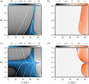
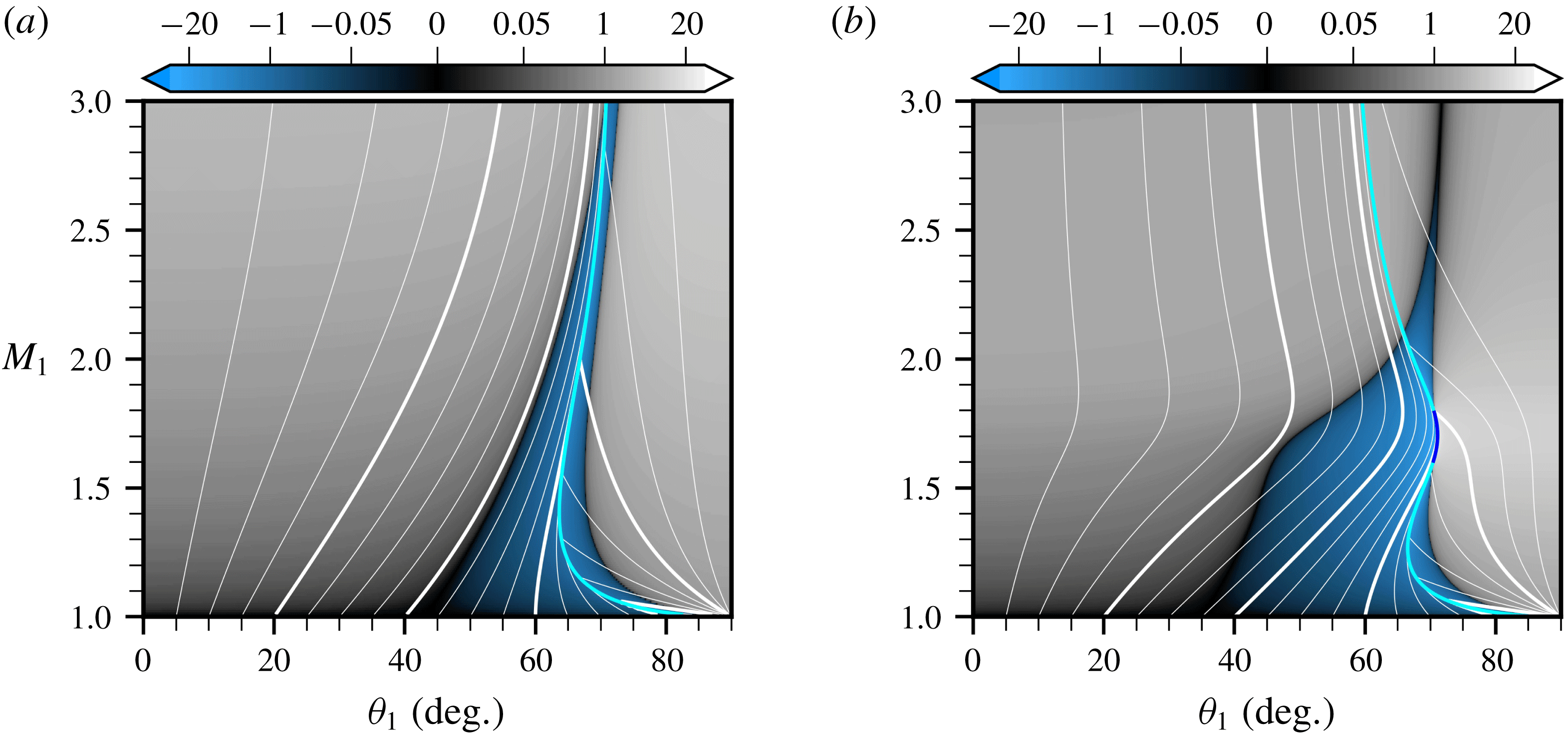
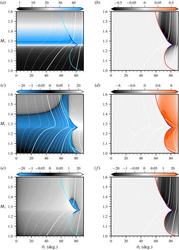
Towards controlling shock-driven acoustic emissions using TCP effects. Acoustic refraction coefficient in the
 $(M_{1},\unicode[STIX]{x1D703}_{1})$
plane:
 $\text{Re}(\unicode[STIX]{x1D712}_{a^{+}})$
(a,c),
 $\text{Im}(\unicode[STIX]{x1D712}_{a^{+}})$
(b,d). Ideal (a,b) versus vdW (c,d) gases with
 $\bar{p}_{1}/p_{c}=0.55$
,
 $\bar{T}_{1}/T_{c}=1.00$
and
 $c_{v}/R=78.2$
. The light blue (a,c) and red (b,d) lines indicate
 $\unicode[STIX]{x1D703}_{1c}(M_{1})$
and the dark blue lines
 $\unicode[STIX]{x1D703}_{1dk}(M_{1})$
. The network of white lines give iso-
 $\unicode[STIX]{x1D703}_{2}$
values in the range
 $[10\text{}^{\circ },170\text{}^{\circ }]$
from left to right (thin lines are spaced by
 $10\text{}^{\circ }$
, thick lines by
 $40\text{}^{\circ }$
). Note the region where
 $\text{Re}(\unicode[STIX]{x1D712}_{a^{+}})\approx 0$
(in black) emerging from the
 $M_{1}\approx 1.35$
mark in the vdW case and extending over
 $20\text{}^{\circ }$
in
 $\unicode[STIX]{x1D703}_{2}$
, defining a ‘cone of silence’ in the emitted sound.

3.1 Cones of silence
The real and imaginary parts of
 $\unicode[STIX]{x1D712}_{a^{+}}$
along the compression branch of the
 ${\mathcal{H}}$
line starting from
 $\bar{p}_{1}/p_{c}=0.55$
and
 $\bar{T}_{1}/T_{c}=1.00$
are shown in figure 2 for both the ideal and vdW gases (the actual
 ${\mathcal{H}}$
line is shown in figure 8). These
 $(M_{1},\unicode[STIX]{x1D703}_{1})$
maps extend figure 14(a) in Alferez & Touber (Reference Alferez and Touber2017a
) (where
 $\unicode[STIX]{x1D703}_{1}=0$
) to all incidence angles (
 $\unicode[STIX]{x1D703}_{1}\in [0,\unicode[STIX]{x03C0}/2]$
).
At zero incidence,
 $\unicode[STIX]{x1D712}_{a^{+}}$
is proportional to
 $\text{sign}(h)[(\unicode[STIX]{x2202}\bar{p}_{2}/\unicode[STIX]{x2202}\bar{\unicode[STIX]{x1D717}}_{2})_{\bar{\unicode[STIX]{x1D717}}_{1},\bar{p}_{1}}+(\unicode[STIX]{x2202}\bar{p}_{2}/\unicode[STIX]{x2202}\bar{\unicode[STIX]{x1D717}}_{1})_{\bar{\unicode[STIX]{x1D717}}_{2},\bar{p}_{1}}]$
(for stable shocks, i.e.
 $-1<h<1+2M_{2}$
). In ideal gases, this term is always strictly positive: acoustic waves in the normal direction to the shock are always emitted, and are in phase with the incoming perturbation. In contrast, the vdW case is chosen such that the sum vanishes twice along the
 ${\mathcal{H}}$
line (the two dark regions in
 $\text{Re}(\unicode[STIX]{x1D712}_{a^{+}})$
). Therefore, acoustic emission in the normal direction to the shock can be suppressed for two values of
 $M_{1}$
. Note that any intermediate value produces acoustic waves in opposite phase to that of the incoming perturbation (see the blue
 $\text{Re}(\unicode[STIX]{x1D712}_{a^{+}})<0$
region near
 $\unicode[STIX]{x1D703}_{1}=0$
).
The
 $\text{Re}(\unicode[STIX]{x1D712}_{a^{+}})=0$
contours emerging at
 $\unicode[STIX]{x1D703}_{1}=0$
extend at almost constant
 $M_{1}$
values over a range of incidence angles (i.e. in the
 $\unicode[STIX]{x1D703}_{1}$
direction). To this
 $\unicode[STIX]{x1D703}_{1}$
range corresponds a
 $\unicode[STIX]{x1D703}_{2}$
range (shown by the white lines) over which no or very weak acoustic waves are emitted. Thus, the sound produced by the impinging entropy mode at these
 $M_{1}$
values will be nearly suppressed within a wedge centred about the normal direction to the shock. For this particular
 ${\mathcal{H}}$
line, this wedge extends from approximately
 $-20\text{}^{\circ }$
to
 $+20\text{}^{\circ }$
. In three-dimensional space, this will translate into a quiet cone, or ‘cone of silence’. This is to contrast with the ideal-gas map, where the region in the normal direction to the shock is home to some of the loudest sounds, whilst a quiet wedge forms in the direction normal to the flow (as shown by the
 $\text{Re}(\unicode[STIX]{x1D712}_{a^{+}})=0$
region that tracks the
 $\unicode[STIX]{x1D703}_{2}\approx 90\text{}^{\circ }$
iso-contour). This quiet wedge precedes the transition to the non-propagating regime across which
 $\text{Re}(\unicode[STIX]{x1D712}_{a^{+}})$
reaches a local (negative) minimum (in blue), as documented by Ribner (Reference Ribner1954), Mahesh et al. (Reference Mahesh, Lele and Moin1997), Fabre et al. (Reference Fabre, Jacquin and Sesterhenn2001), Larsson & Lele (Reference Larsson and Lele2009), Wouchuk et al. (Reference Wouchuk, Huete and Velikovich2009). Note that the ideal-gas map is provided over a greater range of
 $M_{1}$
values to illustrate its relative monotonicity over a range of shock speeds, as opposed to the vdW gas (however,
 $\unicode[STIX]{x1D703}_{1c}$
is not a monotonous function of
 $M_{1}$
, as seen by the presence of a local minimum at
 $M_{1}\approx 1.4$
, also shown in Quadros et al.
Reference Quadros, Sinha and Larsson2016).
Thus, non-ideal-gas effects can give much freedom over the properties of the
 $\text{Re}(\unicode[STIX]{x1D712}_{a^{+}})=0$
contours. These ‘contours of silence’ can break free from simply tracking a
 $\unicode[STIX]{x1D703}_{2}<\unicode[STIX]{x1D703}_{2c}$
contour (ideal gas) and instead be made to explore the entire
 $\unicode[STIX]{x1D703}_{2}$
range, from zero to far into the non-propagative regime (
 $\unicode[STIX]{x1D703}_{2}>\unicode[STIX]{x1D703}_{2c}$
). Remarkably, this is achieved for variations in shock speeds of just a few per cent (see figure 2). Undoubtedly, this observation will have significant implications on the directivity (and controllability) of the emitted sound in shock/turbulence interactions. The transition from the ideal-gas behaviour to one that can be controlled is illustrated in figure 3 by tracking two
 ${\mathcal{H}}$
lines starting at same pre-shock pressures as in figure 2 but more diluted states. The contours of silence are seen to depart from their ideal-gas properties at larger incidence first. This suggests that the one-dimensional analysis presented in Alferez & Touber (Reference Alferez and Touber2017a
) gives the most restrictive picture of non-ideal-gas effects. Multi-dimensional interactions first display their non-ideal-gas ‘pathologies’ at non-zero incidence angles. This attribute is directly related to the curvature of the
 ${\mathcal{H}}$
line, particularly the imminent existence of a sonic point along the
 ${\mathcal{H}}$
line or the neighbouring ones (thereby pushing
 $\unicode[STIX]{x1D703}_{1c}\rightarrow \unicode[STIX]{x03C0}/2$
at a given
 $M_{1}>1$
value, which then acts as a ‘focal’ point on the
 $\unicode[STIX]{x1D703}_{2}(\unicode[STIX]{x1D703}_{1},M_{1})$
map).
Emergence of the silent cone for
 ${\mathcal{H}}$
lines approaching the TCP:
 $(M_{1},\unicode[STIX]{x1D703}_{1})$
maps of
 $\text{Re}(\unicode[STIX]{x1D712}_{a^{+}})$
for the vdW gas with
 $c_{v}/R=78.2$
at
 $\bar{p}_{1}/p_{c}=0.55$
and
 $\bar{\unicode[STIX]{x1D717}}_{1}/\unicode[STIX]{x1D717}_{c}=10$
(a),
 $\bar{\unicode[STIX]{x1D717}}_{1}/\unicode[STIX]{x1D717}_{c}=5$
(b). See figure 2 for full caption and case
 $\bar{\unicode[STIX]{x1D717}}_{1}/\unicode[STIX]{x1D717}_{c}=3.9$
.

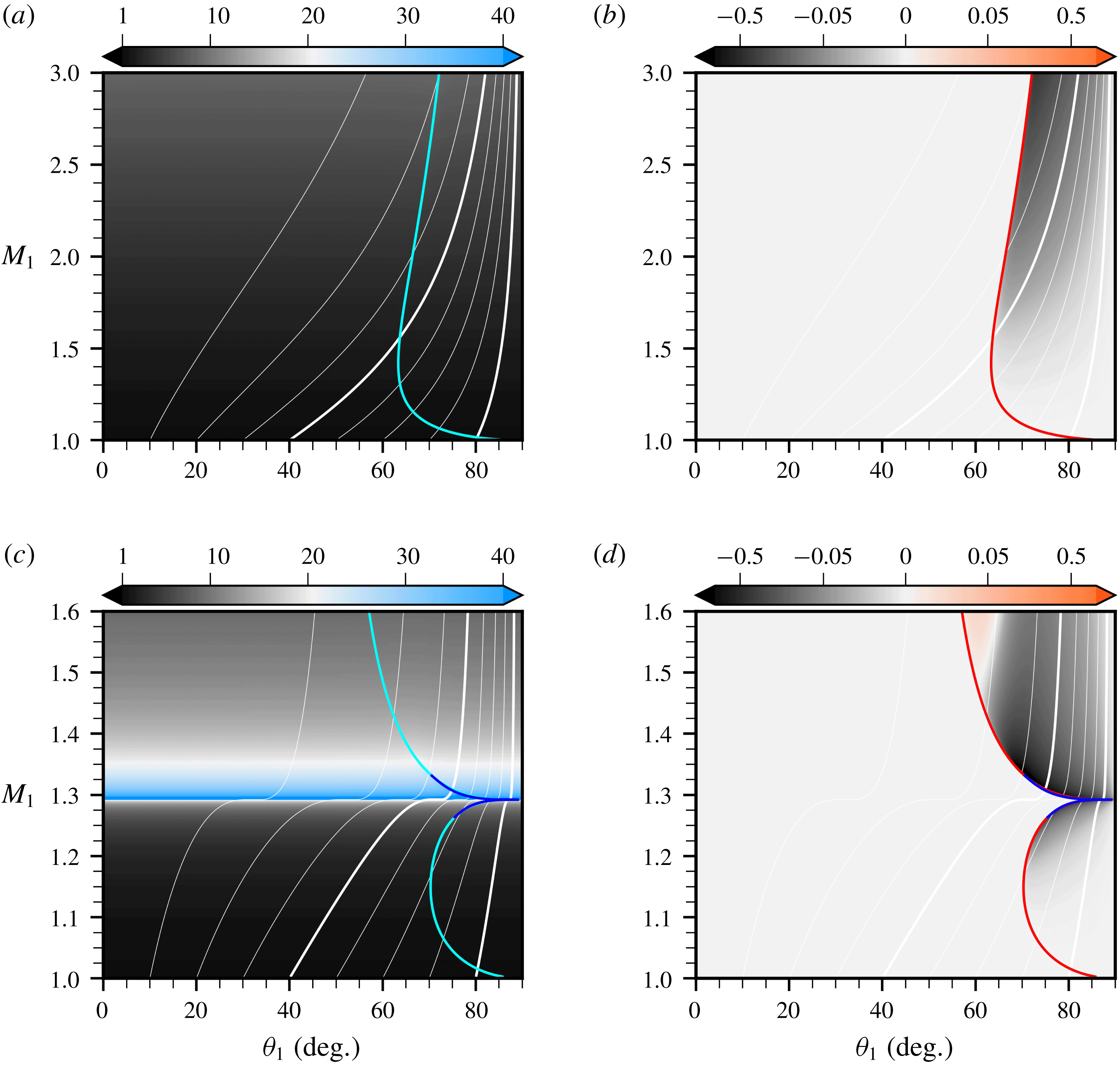
3.2 Selective amplifiers
The pre-shock entropy perturbation is transferred into a post-shock entropy perturbation. The associated transfer functions,
 $\unicode[STIX]{x1D712}_{s}$
, are shown in figure 4. The
 $\text{Re}(\unicode[STIX]{x1D712}_{s})$
maps suggest that one-dimensional results (i.e. obtained for
 $\unicode[STIX]{x1D703}_{1}=0$
) hold regardless of the incidence angles (i.e. the maps are relatively uniform in
 $\unicode[STIX]{x1D703}_{1}$
). This observation implies that, for a given shock speed, the refracted entropy perturbation inherits the same geometrical properties as the incident perturbation, albeit the compression (or stretching) along the flow direction due to the base-flow compression ratio. Furthermore, this observation also implies that the results discussed in Alferez & Touber (Reference Alferez and Touber2017a
) remain valid in multi-dimensions, namely: (i) entropy modes may be amplified by several orders of magnitude over a narrow range of Mach numbers (contrary to ideal gases where the amplification is an increasing function of
 $M_{1}$
); (ii) if the curvature of the
 ${\mathcal{H}}$
line gives rise to a sonic point, then the admissible path is discontinuous and so is the transfer function. Non-ideal shocks can therefore selectively amplify entropy modes. This occurs for example near the
 $M_{1}\approx 1.29$
mark in figure 4 (e.g. blue band corresponding to amplification factors greater than
 $40$
– this is to compare with figure 10(a) in Alferez & Touber Reference Alferez and Touber2017a
). Thus, the curvature of the
 ${\mathcal{H}}$
line plays a central role in transmitting and amplifying entropy modes across the shock, and could be used to promote certain structures in turbulent flows with base flows such that the post-shock state lies near a sonic point.
Towards large and selective entropy-mode amplifications across the shock. Entropy refraction coefficient in the
 $(M_{1},\unicode[STIX]{x1D703}_{1})$
plane:
 $\text{Re}(\unicode[STIX]{x1D712}_{s})$
(a,c),
 $\text{Im}(\unicode[STIX]{x1D712}_{s})$
(b,d). Ideal (a,b) versus vdW (c,d) gases with
 $\bar{p}_{1}/p_{c}=0.55$
,
 $\bar{T}_{1}/T_{c}=1.00$
and
 $c_{v}/R=78.2$
. The light blue (a,c) and red (b,d) lines indicate
 $\unicode[STIX]{x1D703}_{1c}(M_{1})$
and the dark blue lines
 $\unicode[STIX]{x1D703}_{1dk}(M_{1})$
. The network of white lines give iso-
 $\unicode[STIX]{x1D703}_{3}$
values in the range
 $[10\text{}^{\circ },80\text{}^{\circ }]$
from left to right (thin lines are spaced by
 $10\text{}^{\circ }$
, thick lines by
 $40\text{}^{\circ }$
). Note the ‘jump’ in
 $\text{Re}(\unicode[STIX]{x1D712}_{s})$
(vdW case) corresponding to a discontinuity in the admissible path along the
 ${\mathcal{H}}$
line (see Alferez & Touber Reference Alferez and Touber2017a
, for details) and the uniformity of the response to the incidence angle.

3.3 Vorticity generators
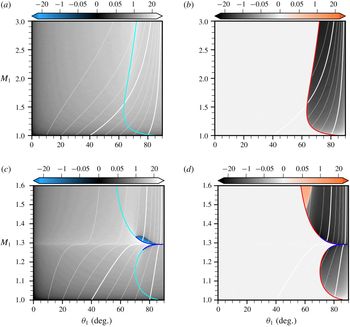
Towards controlling shock-induced energy transfers into solenoidal kinetic energy. Vorticity refraction coefficient in the
 $(M_{1},\unicode[STIX]{x1D703}_{1})$
plane:
 $\text{Re}(\unicode[STIX]{x1D712}_{\unicode[STIX]{x1D6FA}})$
(a,c),
 $\text{Im}(\unicode[STIX]{x1D712}_{\unicode[STIX]{x1D6FA}})$
(b,d). Ideal (a,b) versus vdW (c,d) gases with
 $\bar{p}_{1}/p_{c}=0.55$
,
 $\bar{T}_{1}/T_{c}=1.00$
and
 $c_{v}/R=78.2$
. The light blue (a,c) and red (b,d) lines indicate
 $\unicode[STIX]{x1D703}_{1c}(M_{1})$
and the dark blue lines
 $\unicode[STIX]{x1D703}_{1dk}(M_{1})$
. The network of white lines give iso-
 $\unicode[STIX]{x1D703}_{3}$
values in the range
 $[10\text{}^{\circ },80\text{}^{\circ }]$
from left to right (thin lines are spaced by
 $10\text{}^{\circ }$
, thick lines by
 $40\text{}^{\circ }$
). Note the ‘jump’ in
 $\text{Re}(\unicode[STIX]{x1D712}_{\unicode[STIX]{x1D6FA}})$
(vdW case) before
 $M_{1}\approx 1.3$
, after which the refraction coefficient becomes both large and sensitive to the incidence angle, particularly past or around the critical angle.

Unlike in one dimension, the refraction problem in multi-dimensions enables the production of shear modes, corresponding to a production of solenoidal kinetic energy. The generation coefficients in
 $(M_{1},\unicode[STIX]{x1D703}_{1})$
space are shown in figure 5. The ideal-gas map is similar to that of Mahesh et al. (Reference Mahesh, Lele and Moin1997), despite the different heat-capacity ratios used (
 $\unicode[STIX]{x03B3}=1.013$
here, instead of
 $1.4$
). Vorticity production increases monotonically with incidence angle up to the acoustic critical angle, from which the imaginary part of
 $\unicode[STIX]{x1D712}_{\unicode[STIX]{x1D6FA}}$
is negative and of similar magnitude as for the real part. These features remain unchanged along the
 ${\mathcal{H}}$
line.
In contrast, the distortion of the
 ${\mathcal{H}}$
line by non-ideal-gas effects strongly influences vorticity production. The amplitude of both
 $\text{Re}(\unicode[STIX]{x1D712}_{\unicode[STIX]{x1D6FA}})$
and
 $\text{Im}(\unicode[STIX]{x1D712}_{\unicode[STIX]{x1D6FA}})$
can be significantly higher than in ideal gases, in addition to their sensitivity to changes in both
 $\unicode[STIX]{x1D703}_{1}$
and
 $M_{1}$
. The sensitivity to
 $M_{1}$
mirrors that of
 $\unicode[STIX]{x1D712}_{a^{+}}$
and
 $\unicode[STIX]{x1D712}_{s}$
, and is exacerbated for discontinuous admissible
 ${\mathcal{H}}$
line (e.g. across the BZT region of a dense gas). The sensitivity to
 $\unicode[STIX]{x1D703}_{1}$
combines the ideal-gas behaviour (i.e. tendency to increase near the acoustic critical angle) with the existence of a DK angle. This can be seen for example at
 $\unicode[STIX]{x1D703}_{1}\approx 70\text{}^{\circ }$
and
 $M_{1}\approx 1.33$
where
 $\unicode[STIX]{x1D703}_{1dk}\approx \unicode[STIX]{x1D703}_{1c}$
(the generation coefficient
 $\text{Re}(\unicode[STIX]{x1D712}_{\unicode[STIX]{x1D6FA}})$
can increase by orders of magnitude in these confined regions of
 $(M_{1},\unicode[STIX]{x1D703}_{1})$
space). Interestingly, the sign of
 $\text{Re}(\unicode[STIX]{x1D712}_{\unicode[STIX]{x1D6FA}})$
changes in that region past the critical angle. Whilst the sign can be related to the sign of the produced shear wave, it is not straightforward to see this directly from the
 $(M_{1},\unicode[STIX]{x1D703}_{1})$
map due to the additional contributions of the eigenvector components. A similar argument holds for the change of sign in
 $\text{Im}(\unicode[STIX]{x1D712}_{\unicode[STIX]{x1D6FA}})$
at higher Mach. The net impact on the solenoidal field will be illustrated later (e.g. figure 8).
Remarkably, the curvature of the
 ${\mathcal{H}}$
line offers a degree of freedom by which more intense solenoidal modes can be produced. This remark has practical implications since intense shear waves transition to turbulence more easily and therefore mixing could be promoted via non-ideal shocks. This is illustrated next using a density spot.
4 Energy transfers triggered by entropy spots
Interactions of entropy fluctuations with shocks are common to many real-life scenarios: from cosmological (e.g. shocked interstellar medium) to microscopic (e.g. micronisation by rapid expansion process) scales. Such interactions repeatedly occur in propulsion (e.g. combustion chamber) and power generation (e.g. organic Rankine cycle (ORC) turbines) systems. It is therefore of particular interest to study how the energy of the entropy perturbation is transferred to the fluctuating post-shock kinetic energy. In the linear regime, the refraction process is entirely determined by the previously described transmission and generation maps via linear combinations. Perhaps the most obvious perturbation bearing both a degree of realism whilst maintaining a degree of simplicity is the entropy spot discussed in Fabre et al. (Reference Fabre, Jacquin and Sesterhenn2001). It is realistic in that complex interactions can be seen as the sum of entropy spots of various sizes and strengths. It is simple in that the azimuthal symmetry of the spot excites all incidences angles with equal strength, easing the connection with the
 $(M_{1},\unicode[STIX]{x1D703}_{1})$
maps from § 3. The objective of this section is twofold: first, to illustrate the singular response of non-ideal shocks to the entropy-spot perturbation; second, to illustrate the predictive nature of the linear theory.
4.1 Flow configuration and methodology
A 1 % low-density perturbation with uniform pressure and velocity is introduced in a gas at rest and impinged by a shock wave, i.e.
 $\unicode[STIX]{x1D741}_{1}=\bar{\unicode[STIX]{x1D741}}_{1}+\unicode[STIX]{x1D700}\unicode[STIX]{x1D741}_{1}^{\prime }$
with
 $\unicode[STIX]{x1D700}=10^{-2}$
. The perturbation assumes a Gaussian shape with unitary mid-high width and amplitude:
 $$\begin{eqnarray}\unicode[STIX]{x1D741}_{1}^{\prime }=\left[\begin{array}{@{}c@{}}\unicode[STIX]{x1D70C}^{\prime }\\ \boldsymbol{u}^{\prime }\\ p^{\prime }\end{array}\right]=\left[\begin{array}{@{}c@{}}-\text{exp}\left\{-{\displaystyle \frac{1}{2}}\left[\left({\displaystyle \frac{x-x_{0}}{r_{0}}}\right)^{2}+\left({\displaystyle \frac{y-y_{0}}{r_{0}}}\right)^{2}\right]\right\}\\ \mathbf{0}\\ 0\end{array}\right],\end{eqnarray}$$
where
 $(x_{0},y_{0})$
are the coordinates of the centre of the Gaussian spot and
 $r_{0}\equiv r\text{}_{0}^{\ast }/\ell \text{}^{\ast }$
with
 $r\text{}_{0}^{\ast }=\ell \text{}^{\ast }/(2\sqrt{2\text{ln}2})$
to ensure a full width at half-maximum of length
 $\ell \text{}^{\ast }$
(i.e. the reference length scale used to obtain the dimensionless form of the equations, see § 2.2).
The current study builds on that of Fabre et al. (Reference Fabre, Jacquin and Sesterhenn2001) for ideal gases by commenting on salient effects associated with the curvature of the
 ${\mathcal{H}}$
line, as discussed in § 3. The Gaussian profile enables the study of the anisotropic nature of the refracted field since it precludes forcing any particular incident angle
 $\unicode[STIX]{x1D703}_{1}$
. A series of shock waves (i.e. with different speeds and pre-shock states) is first considered using the van der Waals EOS. The resulting analytical expressions allow for an easy comparison between theory and numerical simulations of the Euler equations. A graphical summary is given in figures 8 and 13. A more realistic and accurate EOS (i.e. Span–Wagner for siloxane D6) is investigated (solely from the perspective of the linear theory) in a separate section (see § 5) to illustrate the generality of the results obtained using the vdW EOS.
4.1.1 Linear interaction analysis
Analytical solutions to the density-spot/shock wave interaction problem are built based on the LIA formalism first proposed by Ribner (Reference Ribner1954) to study vortex/shock interactions and extended by Fabre et al. (Reference Fabre, Jacquin and Sesterhenn2001) to the density-spot/shock interaction. A Fourier transform is applied to the initial density spot and the interaction of the resulting individual wave modes considered independently from each other. The analytical derivation with the Gaussian spot is facilitated by the analytical nature of its Fourier transform. The refracted solution is obtained as the superposition of each individual wave-mode response. This superposition is done through a numerical integration in Fourier space. Details of the procedure are given in Fabre et al. (Reference Fabre, Jacquin and Sesterhenn2001). In the present study, the general non-ideal gas transmission and generation coefficients, obtained in § 2.3, are used as input of the above superposition procedure. The density-spot/shock wave interaction problem is therefore solved for an arbitrary equation of state. Note that for cases satisfying condition (2.14) (existence of a DK angle), the summation procedure in Fourier space fails (
 $\unicode[STIX]{x1D712}_{s}$
,
 $\unicode[STIX]{x1D712}_{a^{+}}$
,
 $\unicode[STIX]{x1D712}_{\unicode[STIX]{x1D6FA}}$
are singular). Instead, results from direct numerical simulations of the Euler equations will be presented for these cases (the recombination of the modes is not singular, as discussed by Semenko Reference Semenko2017; Semenko & Semenko Reference Semenko and Semenko2017).
4.1.2 Direct numerical simulations
The LIA results are compared and extended with solutions of the density-spot/shock wave interaction obtained by direct numerical integration of the two-dimensional Euler equations on a Cartesian grid with
 $3048\times 4464$
points. The equations are integrated in time explicitly using a third-order total variation diminishing Runge–Kutta scheme (Shu & Osher Reference Shu and Osher1989). Spatial derivatives are evaluated with a fourth-order centred finite difference dispersion-relation-preserving scheme (Tam & Webb Reference Tam and Webb1993) using a 13-point stencil (a four points per wavelength cutoff is used for the dispersion optimisation process). The centred finite difference scheme is stabilised with a centred 13-point eighth-order explicit discrete filter optimised in spectral space to minimise small-scale dissipation up to a cutoff wavenumber, following the methodology developed by Bogey & Bailly (Reference Bogey and Bailly2004) (a five points per wavelength cutoff is used).
The shock is captured by adding explicit bulk-viscosity and thermal-conductivity terms to the momentum and energy equations in the region of the shock (easily located due to its fixed and isolated nature), in the same spirit as Cook & Cabot (Reference Cook and Cabot2004), Kawai & Lele (Reference Kawai and Lele2008), Kawai, Shankar & Lele (Reference Kawai, Shankar and Lele2010), Terashima, Kawai & Koshi (Reference Terashima, Kawai and Koshi2013). Contrary to these works, where artificial transport coefficients are dynamically set, the present work uses constant and uniform values to spread the shock over a target number of points so as to directly control spurious-noise levels. Whilst shock/turbulence interaction studies operate with noise levels of approximately 1 % of the jump amplitude (Johnsen et al. Reference Johnsen, Larsson, Bhagatwala, Cabot, Moin, Olson, Rawat, Shankar, Sjögreen, Yee, Zhong and Lele2010), the present work is based on noise levels set to 0.01 % of the jump amplitude. This is necessary in order to capture the refraction of a perturbation set at 1 % of the pre-shock state (and the presumed ability of non-ideal shocks to suppress the emitted sound for example).
A mapping between the computational grid and the physical space is applied (grid stretching) to control the actual shock thickness,
 $\unicode[STIX]{x1D6E5}$
, in physical space. In this work, the numerical shock is set to span
 $25$
grid points but is mapped to a physical space of
 $\unicode[STIX]{x1D6E5}/\ell =2\times 10^{-2}$
(where
 $\ell$
is the incoming perturbation mid-high width). This methodology has been validated in one-dimensional flows in Alferez & Touber (Reference Alferez and Touber2017b
). Supersonic inflow and non-reflective boundary conditions (Okong’o & Bellan Reference Okong’o and Bellan2002) are used in the streamwise direction. Periodic boundary conditions (with periodic length
 $L_{y}/\ell =90$
) are imposed along the shock direction.
4.2 Internal to kinetic energy transfers
Time lapses extracted from the numerical simulations of the entropy-spot/shock interactions (
 $\bar{p}_{1}/p_{c}=0.55$
and
 $\bar{T}_{1}/T_{c}=1.0$
). Ideal gas (a, movie 1) with
 $M_{1}=1.33907$
; vdW gas with
 $M_{1}=1.34900$
(b, movie 2) and
 $M_{1}=1.29222$
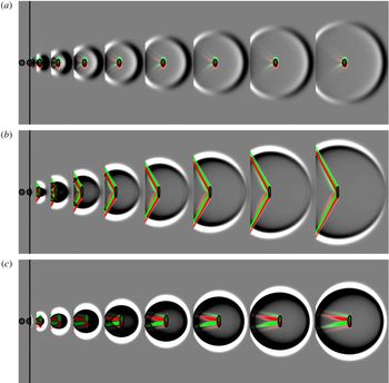
(c, movie 3). Length scales and colour bars (given in figure 7) are identical for each strip. Movies are available online at https://doi.org/10.1017/jfm.2019.25.

4.2.1 Generic transfers
Instantaneous refracted field in ideal gas for
 $M_{1}=1.33907$
and
 $\unicode[STIX]{x03B3}=1.013$
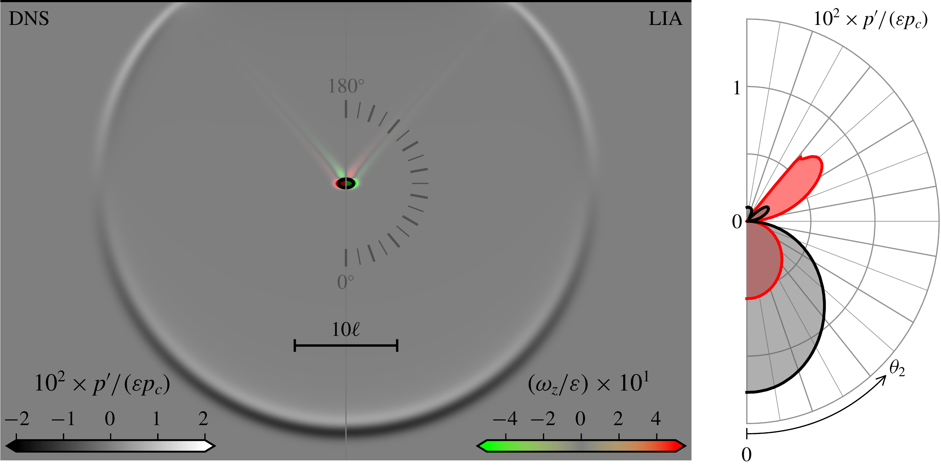
. Panel (a) gives the vorticity (
 $\unicode[STIX]{x1D714}_{z}\equiv (\unicode[STIX]{x1D735}\text{}^{\ast }\times \boldsymbol{u}\text{}^{\ast })\boldsymbol{\cdot }\boldsymbol{e}_{z}\,\ell \text{}^{\ast }/\sqrt{p_{c}/\unicode[STIX]{x1D70C}_{c}}$
, in colour) and fluctuating pressure (
 $p^{\prime }$
, in grey scale) fields. The isocontour
 $\unicode[STIX]{x1D70C}^{\prime }/\bar{\unicode[STIX]{x1D70C}}_{2}=10^{-1}\unicode[STIX]{x1D700}$
(black line with internal shading) is also shown to visualise the refracted entropy spot (with the LIA only showing the entropy-mode contribution to
 $\unicode[STIX]{x1D70C}^{\prime }$
). The field is cut along the symmetry line to show the numerical simulation (DNS) on the left against the linear theory (LIA) on the right (each side corresponds to the true field of view, i.e. no mirroring is applied, hence the opposite signs on
 $\unicode[STIX]{x1D714}_{z}$
). Panel (b) gives the maximum (red) and minimum (black) pressure fluctuations in terms of observation angles
 $\unicode[STIX]{x1D703}_{2}\in [0,\unicode[STIX]{x03C0}]$
as seen from an observer attached to the refracted spot in the numerical simulation (solid lines) and linear theory (filled contours). The LIA is in perfect agreement with the DNS.

The compression front turns the low-density spot into an ellipse. The spot induces a deformation of the shock that runs in both directions along the front (with speed
 $\sqrt{c_{2}^{2}-\bar{u}_{2}^{2}}$
) so as to emit a ‘cylindrical’ acoustic wave together with ‘parallel’ shear waves. Figure 6 presents time snapshots (extracted from the numerical simulations) of the perturbed pressure, density and vorticity fields for varying upstream Mach numbers in both ideal and non-ideal gases. The generated vorticity field is made of a vortex dipole and two distinct shear waves corresponding to the local maximum of
 $|\unicode[STIX]{x1D712}_{\unicode[STIX]{x1D6FA}}|$
around the critical acoustic angle. In the linear regime, the dipole and shear waves are advected as a frozen pattern at speed
 $\bar{u}_{2}$
(see figure 6). Nonlinear effects eventually distort the pattern and some early signs are visible in the vdW case at
 $M_{1}=1.29222$
, e.g. the symmetry of the elliptic density contour is progressively broken (see also appendix C for the
 $M_{1}=1.34900$
case with a 10 % perturbation). The cylindrical acoustic wave is centred around the refracted spot and propagates away from it at speed
 $c_{2}$
.
This generic topology (compressed spot, vortex dipole, linear shear waves, cylindrical acoustic wave) is maintained regardless of the thermodynamic properties of the substance. The detailed structure and amplitude of the shear and acoustic waves, however, depend on the equation of state (more generally on the curvature of the
 ${\mathcal{H}}$
lines). Owing to the axisymmetric nature of the perturbation, the shear- and acoustic-wave properties can be directly anticipated from the
 $(M_{1},\unicode[STIX]{x1D703}_{1})$
maps (this will prove useful when interpreting the non-ideal-gas results). To do so, one must use the geometrical reconstruction proposed by Ribner (Reference Ribner1954) and extended by Fabre et al. (Reference Fabre, Jacquin and Sesterhenn2001). A key aspect is to select the polar coordinates system attached to the refracted entropy spot, with
 $\unicode[STIX]{x1D703}=0^{\circ }$
placed in the forward direction (see the grey coloured compass in figure 7). The angular values in this polar coordinates correspond to
 $\unicode[STIX]{x1D703}_{2}$
and
 $\unicode[STIX]{x1D703}_{3}$
(the white lines in figure 2 to 5). For example, reading the
 $M_{1}=1.33907$
line in figure 2 for the ideal gas reveals that the cylindrical acoustic wave is more intense in the flow direction (
 $\unicode[STIX]{x1D703}=0^{\circ }$
), vanishes at
 $\unicode[STIX]{x1D703}=90^{\circ }$
, and changes sign afterwards, as also seen in figure 7.
The ideal-gas response (figure 6
a) reproduces the flow topology commented in Fabre et al. (Reference Fabre, Jacquin and Sesterhenn2001). As expected, the characteristics of the corresponding acoustic pressure perturbation reflects the anisotropic nature of the interaction commented in § 3.1. At this Mach number (
 $M_{1}=1.33907$
) the value of
 $\text{Re}(\unicode[STIX]{x1D712}_{a^{+}})$
is positive for
 $\unicode[STIX]{x1D703}_{1}=0^{\circ }$
. This positive sign implies that, at the shock location, the generated acoustic perturbation is in phase with the impinging entropy perturbation, i.e. the generated pressure fluctuation will carry the sign of
 $\unicode[STIX]{x1D70C}_{1}^{\prime }$
at the shock location. Depending on the incidence angle, the sign of
 $\text{Re}(\unicode[STIX]{x1D712}_{a^{+}})$
may change and out-of-phase pressure fluctuations be generated at the shock. In the Gaussian-spot problem, the sign of the generated acoustic fluctuations can then be anticipated near the shock front at the early stage of the interaction. For the ideal gas, the in-phase part of the propagating acoustic wave (i.e. for low values of
 $\unicode[STIX]{x1D703}_{2}$
) is indeed a negative pressure fluctuation (i.e. inherited from the impinged negative density fluctuation, see (4.1)). Furthermore, at this Mach number in the
 $(M_{1},\unicode[STIX]{x1D703}_{1})$
map,
 $\text{Re}(\unicode[STIX]{x1D712}_{a^{+}})$
changes sign at
 $\unicode[STIX]{x1D703}_{2}\approx 90^{\circ }$
. The generated acoustic wave hence features a silent wedge around this direction and a sign change for the fluctuating pressure is observed for
 $\unicode[STIX]{x1D703}_{2}$
exceeding
 $90^{\circ }$
. The resulting acoustic emission is therefore similar to that of an acoustic dipole.
The formation of shear waves (following the hot-spot refraction) is interpreted as a transfer from internal energy to solenoidal kinetic energy. Similarly, the emitted acoustic wave is interpreted as a transfer to dilatational kinetic energy. The next two sections demonstrate that the thermal equation of state can be used to control the transfer to both types of kinetic energy, as suggested by figure 6.
4.2.2 Controlling the dilatational kinetic energy
In ideal gases, transfers of entropy (internal energy) perturbations to acoustic (dilatational kinetic) energy increase monotonously with the shock speed (
 $M_{1}$
), as seen from
 $\text{Re}(\unicode[STIX]{x1D712}_{a^{+}})$
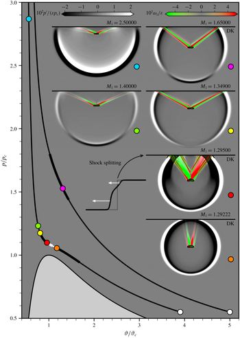
in figure 2. Dense vapours considered here provide an additional degree of freedom (namely, the proximity of the post-shock state to a saddle point on the isotherm map) allowing the transfers to dilatational kinetic energy to be controlled. Section 3.1 has for example anticipated the possibility of suppressing the sound emitted in the shock-normal direction. This is illustrated in figure 6 (b). Conversely, transfers to the dilatational kinetic energy may be promoted, as shown in figure 6 (c). Note that the variety of energy transfers shown here is achieved for variations in shock speeds of less than
 $5\,\%$
(such degree of control is simply not possible in ideal substances). This feat is achievable thanks to the curvature of the selected
 ${\mathcal{H}}$
line, shown in figure 8. The loudest field is obtained when approaching a sonic point (
 $M_{2}\approx 0.99$
at
 $M_{1}=1.29222$
, as may be seen from the near-circular shape of the acoustic wave – the perturbation along the shock front is almost stationary, i.e.
 $\sqrt{c_{2}^{2}-\bar{u}_{2}^{2}}\ll 1$
). This is also visible from the large values of
 $|\text{Re}(\unicode[STIX]{x1D712}_{a^{+}})|$
(figure 2). Past the non-admissible section (shown in white in figure 8), the quietest field is obtained. Going further along the
 ${\mathcal{H}}$
line, acoustic fields similar to that of the ideal gas may be recovered (e.g.
 $M_{1}=1.40000$
), and even suppressed along the shock (e.g.
 $M_{1}=2.50000$
). It is therefore evident that the magnitude of the post-shock dilatational kinetic energy is controllable (note that the present diversity in the emitted acoustic is based on a single
 ${\mathcal{H}}$
line and that further diversity may be obtained from neighbouring operating conditions).
Diversity of refracted spots (obtained by DNS) identified by the coloured circles along the
 ${\mathcal{H}}$
lines originating at
 $\bar{p}_{1}/p_{c}=0.55$
,
 $\bar{T}_{1}/T_{c}=1.00$
; and
 $\bar{p}_{1}/p_{c}=0.55$
,
 $\bar{\unicode[STIX]{x1D717}}_{1}/\unicode[STIX]{x1D717}_{c}=5.0$
(white circles). Non-admissible portions of the
 ${\mathcal{H}}$
lines are shown in white, and those satisfying the DK criterion are made thicker. See figure 7 for further details.

Silencing a shock in the normal direction: vdW gas at
 $M_{1}=1.33907$
(
 $\unicode[STIX]{x03B3}=1.013$
,
 $\bar{p}_{1}/p_{c}=0.55$
,
 $\bar{T}_{1}/T_{c}=1.0$
). See figure 7 for full caption.

The predictability of the linear theory for a 1 % perturbation is evaluated with DNS results in figure 9 at
 $M_{1}=1.33907$
(along the
 ${\mathcal{H}}$
line starting at
 $\bar{p}_{1}/p_{c}=0.55$
,
 $\bar{T}_{1}/T_{c}=1.0$
for a vdW gas with
 $c_{v}/R=78.2$
), the theoretical value for which no sound is emitted in the shock-normal direction (as seen from the vanishing of
 $p^{\prime }$
about the
 $\unicode[STIX]{x1D703}=0^{\circ }$
direction in the LIA). The LIA and DNS are in good agreement (e.g. loudest sound at
 $\unicode[STIX]{x1D703}_{2}\approx 120^{\circ }$
, quietest sound at
 $\unicode[STIX]{x1D703}_{2}\approx 0^{\circ }$
). The acoustic signature in the shock-normal direction is not completely suppressed in the DNS, and contrasts with the perfect LIA–DNS match obtained in ideal gases (for same
 $\unicode[STIX]{x03B3}$
,
 $M_{1}$
values and perturbation amplitude). Silent-shock properties form a path in
 $(p,\unicode[STIX]{x1D717})$
space across families of
 ${\mathcal{H}}$
lines, as shown in figures 15 and 21(b) of Alferez & Touber (Reference Alferez and Touber2017a
), corresponding to just one or two points along a given
 ${\mathcal{H}}$
line. Any finite displacement in
 $(p,\unicode[STIX]{x1D717})$
space suffices to miss the silent-shock properties. The shock-capturing strategy employed here gives a maximum error on
 $\bar{p}_{2}$
and
 $\bar{\unicode[STIX]{x1D717}}_{2}$
(due to the viscous structure of the shock) below 0.001 %, and is not believed to contribute much to the discrepancies. The 1 % perturbation, however, is large enough to provoke displacements in
 $(p,\unicode[STIX]{x1D717})$
space that highlight the local nature of the condition
 $(\unicode[STIX]{x2202}\bar{p}_{2}/\unicode[STIX]{x2202}\bar{\unicode[STIX]{x1D717}}_{2})_{\bar{\unicode[STIX]{x1D717}}_{1},\bar{p}_{1}}=(\unicode[STIX]{x2202}\bar{p}_{2}/\unicode[STIX]{x2202}\bar{\unicode[STIX]{x1D717}}_{1})_{\bar{\unicode[STIX]{x1D717}}_{2},\bar{p}_{1}}$
(recall that the LIA assumes
 $\unicode[STIX]{x1D700}\rightarrow 0$
). The occurrence of nonlinear effects earlier on in
 $\unicode[STIX]{x1D700}$
values (compared to an ideal gas) is discussed further in appendix C. Note that for a constant perturbation amplitude (
 $\unicode[STIX]{x1D700}=10^{-2}$
here), exploring the neighbourhood of a truly silent shock can also deliver quieter refractions (when considering all
 $\unicode[STIX]{x1D703}_{2}$
values), as demonstrated by case
 $M_{1}=1.34900$
(figure 10, DNS), illustrating the degree of control non-ideal fluids may offer on the post-shock sound intensity and directivity.
Silencing a shock further (vdW gas):
 $M_{1}=1.34900$
(DNS) and
 $M_{1}=1.33907$
(LIA) (
 $\unicode[STIX]{x03B3}=1.013$
,
 $\bar{p}_{1}/p_{c}=0.55$
,
 $\bar{T}_{1}/T_{c}=1.0$
). See figure 7 for full caption.

Finally, note that both the silent and loud shocks feature negative values of
 $\text{Re}(\unicode[STIX]{x1D712}_{a^{+}})$
over the entire propagative regime (see the blue region in figure 2). Thus, the observed acoustic signature is that of a monopole (in phase opposition with the incident perturbation), as opposed to the acoustic dipole in ideal gas (in phase with the incident perturbation).
4.2.3 Controlling the solenoidal kinetic energy
In ideal gases, the relative amount of energy transferred (from the entropy spot) to the solenoidal and dilatational kinetic energies is set by the shock speed (and
 $\unicode[STIX]{x03B3}$
). This is no longer the case in non-ideal fluids, as was already commented at the level of the eigenmode basis (see § 2.2). Thus, both the silent and loud shocks studied in the previous section can be associated with either energetic or weak shear waves.
For example, base flows at
 $M_{1}=1.29222$
and
 $M_{1}=1.29500$
(shown in figure 8) both give rise to loud acoustic monopoles, but feature strikingly different post-shock vorticity patterns: the
 $M_{1}=1.29222$
case produces low-amplitude shear waves almost normal to the shock (see figure 6
c and movie 3 for later times as well) whereas the
 $M_{1}=1.29500$
case produces wide and intense vorticity sheets. Both base flows satisfy the DK criterion (see (2.14)), preventing the LIA to be applied at the DK angle.
Note that neither the loud sound nor the wide vorticity sheets of these DK cases should be interpreted as evidence of the so-called ‘spontaneous acoustic emission’ for shocks satisfying the DK criteria (see D’yakov Reference D’yakov1954; Bates Reference Bates2000, for example). A case with no sonic point but satisfying the DK criterion is shown in figure 8 (magenta dot) as counter example (the refracted field is similar to that of the ideal gas), and confirms the work by Semenko (Reference Semenko2017), Semenko & Semenko (Reference Semenko and Semenko2017), i.e. the inapplicability of the LIA at the DK angle is an artefact of the eigenmode decomposition.
Nevertheless, the
 $(M_{1},\unicode[STIX]{x1D703}_{1})$
maps of
 $\unicode[STIX]{x1D712}_{\unicode[STIX]{x1D6FA}}$
in figure 5 may be used to anticipate these results: at
 $M_{1}=1.29222$
,
 $|\text{Re}(\unicode[STIX]{x1D712}_{\unicode[STIX]{x1D6FA}})|$
remains low (of the order of unity) for all post-shock entropy-vorticity-wave angles
 $\unicode[STIX]{x1D703}_{3}$
(there is indeed a maximum towards
 $\unicode[STIX]{x1D703}_{3}=90^{\circ }$
when
 $M_{2}\rightarrow 1$
). In contrast, at
 $M_{1}=1.29500$
(i.e. just after the discontinuity along the admissible
 ${\mathcal{H}}$
line), high
 $|\text{Re}(\unicode[STIX]{x1D712}_{\unicode[STIX]{x1D6FA}})|$
values (of the order of ten) are observed over all incidence angles below the critical acoustic angle, giving rise to the wide vorticity sheets observed in the direct numerical simulations. Simulations of cases with post-shock states set marginally behind the non-admissible segment of the
 ${\mathcal{H}}$
line are prone to shock splitting (see Cramer & Crickenberger Reference Cramer and Crickenberger1991) into two forward-propagating shocks (with the first one being the fastest and delivering a sonic post-shock state, see the actual initial and later shock profiles in figure 8).
Recovering ideal-gas-like features near the TCP: vdW gas at
 $M_{1}=1.40000$
(
 $\unicode[STIX]{x03B3}=1.013$
,
 $\bar{p}_{1}/p_{c}=0.55$
,
 $\bar{T}_{1}/T_{c}=1.0$
). See figure 7 for full caption.

Moving up the
 ${\mathcal{H}}$
line (in
 $M_{1}$
), the silent shock discussed previously is found to come with energetic shear waves. In the nonlinear regime, these shear waves will transition to turbulence (see also appendix C), making the silent shock particularly interesting for applications seeking to reduce shock-induced noise whilst enhancing turbulent mixing (e.g. scramjet, jet engines). The strong shear wave is produced at the acoustic critical angle and beyond (see figure 5). Increasing
 $M_{1}$
further (i.e. to
 $M_{1}=1.40000$
) delivers a flow topology similar to that of the ideal gas: acoustic dipole with (weaker) shear waves positioned around the critical acoustic angle, see figure 11. This can again be anticipated from the refraction coefficient maps in § 3. This case serves as a reminder that it is possible to obtain ideal-gas-like results despite being relatively close to the TCP (this does not mean that theories based on the ideal-gas EOS should be applied there – instead, this is fortuitous and reflects the very local property of the
 ${\mathcal{H}}$
line which mimics that of the ideal gas). The LIA/DNS agreement is indeed less favourable than in the truly ideal-gas scenario, owing to the sensitivity (in
 $M_{1}$
) of the refraction map, which is actually probed by the 1 % perturbation amplitude (see appendix C).
Finally, when considering stronger shocks (e.g.
 $M_{1}=2.50000$
), yet another peculiar vorticity pattern is observed, which is characterised by the presence of additional and distinct shear waves, as shown in figure 12. These are associated with a sign change in
 $\text{Im}(\unicode[STIX]{x1D712}_{\unicode[STIX]{x1D6FA}})$
(red region in figure 5) together with a local maximum in
 $\text{Re}(\unicode[STIX]{x1D712}_{\unicode[STIX]{x1D6FA}})$
over the same region. (These features extend beyond the
 $M_{1}$
range given in figure 5, and in particular for the shock speed shown in figure 12.)
Suppressing the acoustic wave on the shock and adding more shear waves: vdW gas at
 $M_{1}=2.50000$
(
 $\unicode[STIX]{x03B3}=1.013$
,
 $\bar{p}_{1}/p_{c}=0.55$
,
 $\bar{T}_{1}/T_{c}=1.0$
). See figure 7 for full caption. See movie 4 for the corresponding DNS-based animation.

The diversity of the refracted fields, and therefore the associated energy redistribution into dilatational (acoustic) versus solenoidal (vortical) motions, is striking given that it is achieved over shock speed variations of less than
 $10\,\%$
. Whilst the energy redistribution process is locked in ideal gases (it is set by
 $\unicode[STIX]{x03B3}$
and remains virtually unchanged over the range of shock speed considered here), non-ideal thermodynamic properties may unlock these transfers. Shock speed variations of few per cent are achievable in shock/turbulence interactions, suggesting that the post-shock turbulence kinetic energy could be controlled through thermodynamics alone. The linear theory is remarkably accurate in order to identify and select promising configurations. Finally, given that the controllability of shock-induced energy transfers is rooted in the properties of the
 ${\mathcal{H}}$
lines, the results presented here extend beyond dense vapours near the TCP and are applicable to substances featuring similar
 ${\mathcal{H}}$
lines (e.g. shock-induced phase transition, reacting fronts, systems of self-propelled particles).
4.2.4 Energy transfers specific to expansion shocks
Entropy-spot refraction patterns (obtained by DNS) along the
 ${\mathcal{H}}$
line starting at
 $\bar{p}_{1}/p_{c}=1.012$
and
 $\bar{T}_{1}/T_{c}=1.0029$
(white circle) for a vdW gas (for
 $c_{v}/R=78.2$
). The plot follows the same convention as in figure 8 except for the choice of density isocontours (taken at
 $\unicode[STIX]{x1D70C}^{\prime }/\bar{\unicode[STIX]{x1D70C}}_{2}=10^{-4}$
) and clipping of pressure fluctuations (see grey scale colour bar). Note that the pre-shock state is chosen in a positive
 $\unicode[STIX]{x1D6E4}$
region, making weak expansion shocks non-admissible (they fail to satisfy the entropy condition).

A distinctive feature of non-ideal gas dynamics is the ability to steepen expansion waves to form admissible expansion shock waves (Thompson & Lambrakis Reference Thompson and Lambrakis1973; Cramer & Kluwick Reference Cramer and Kluwick1984; Cramer & Sen Reference Cramer and Sen1986; Guardone & Argrow Reference Guardone and Argrow2005; Zamfirescu et al.
Reference Zamfirescu, Guardone and Colonna2008; Guardone et al.
Reference Guardone, Zamfirescu and Colonna2010). This section presents the refraction properties of an expansion shock typically formed for thermodynamic conditions surrounding the BZT region of a dense gas (see
 $\unicode[STIX]{x1D6E4}<0$
region in figure 13). Contrary to classical compression shocks, expansion shocks formed in dense gases possess a maximum strength beyond which no admissible shocks can exist (
 ${\mathcal{H}}$
lines can only be concave over a finite region of
 $(p,\unicode[STIX]{x1D717})$
space to satisfy the thermodynamic constraint that dilute gases converge to the ideal-gas law, see Guardone et al.
Reference Guardone, Zamfirescu and Colonna2010). The corresponding admissible
 ${\mathcal{H}}$
lines are then restricted to finite segments (in
 $(p,\unicode[STIX]{x1D717})$
space), as illustrated for example in figure 13 (admissible sections are shown in black, portions satisfying the DK criteria are made thicker).
Figure 14 gives the
 $(M_{1},\unicode[STIX]{x1D703}_{1})$
map of the refraction coefficients corresponding to the admissible
 ${\mathcal{H}}$
line in figure 13. Some features are similar to that of compression shocks:
 $\text{Re}(\unicode[STIX]{x1D712}_{s})$
does not depend much on the incidence angle, the sonic point on the
 ${\mathcal{H}}$
line (corresponding to the strongest admissible expansion shock) pushes the acoustic critical angle towards
 $\unicode[STIX]{x03C0}/2$
(all modes then become propagative) and acts as a focal point on the map (the refraction coefficients are most sensitive in
 $M_{1}$
there). The strongest vorticity production is observed at the strongest shock and at wide angles, i.e.
 $\unicode[STIX]{x1D703}_{3}>80^{\circ }$
(see case
 $M_{1}=1.29248$
in figure 13 for example). The acoustic field is that of a monopole in phase (the sign of
 $\text{Re}(\unicode[STIX]{x1D712}_{a^{+}})$
is positive across the entire propagating regime). Contrary to compression shocks, the entropy mode is never amplified (
 $\text{Re}(\unicode[STIX]{x1D712}_{s})<1$
) and almost not transmitted when reaching the strongest shock. This implies that achieving a (near) homentropic flow downstream of a strong expansion shock subjected to incoming entropy perturbations is theoretically possible. Also, note that the
 ${\mathcal{H}}$
line near the pre-shock state being non-admissible (owing to the choice of a pre-shock state in a region where
 $\unicode[STIX]{x1D6E4}>0$
), the transmission coefficient is not unitary when
 $M_{1}\rightarrow 1$
(
 $\bar{\unicode[STIX]{x1D717}}_{2}$
does not go to
 $\bar{\unicode[STIX]{x1D717}}_{1}$
in this limit).
Refraction coefficients
 $\unicode[STIX]{x1D712}_{s}$
(a,b),
 $\unicode[STIX]{x1D712}_{a^{+}}$
(c,d) and
 $\unicode[STIX]{x1D712}_{\unicode[STIX]{x1D6FA}}$
(e,f) for expansion shocks in vdW (
 $c_{v}/R=78.2$
) starting from
 $\bar{p}_{1}/p_{c}=1.012$
,
 $\bar{T}_{1}/T_{c}=1.0029$
. Real (a,c,e) and imaginary (b,d,f) parts. See figure 2, 4 and 5 for full caption.

Figure 15 compares the LIA and the DNS at
 $M_{1}=1.2000$
. The acoustic monopole signature and the vorticity fields are in good agreement. Note that owing to the expansion ratio, the refracted pulse is now stretched in the flow direction. This implies that spurious noise (initially unresolved) can expand to wavelengths no longer discriminated by the numerical stabilisation technique (explicit filters in our case). This effect is mitigated here by resolving the artificial shock structure (with approximately 25 points) and refining the mesh to ensure a proper scale separation between the shock thickness and the perturbation wavelength (see § 4.1.2).
The solenoidal field bears the signature of two local maxima in
 $|\text{Re}(\unicode[STIX]{x1D712}_{\unicode[STIX]{x1D6FA}})|$
. The first (and weaker) one occurs below the acoustic critical angle. The second occurs past the acoustic critical angle (and is further reinforced by
 $|\text{Im}(\unicode[STIX]{x1D712}_{\unicode[STIX]{x1D6FA}})|$
) with an associated wave vector angle at
 $\unicode[STIX]{x03C0}/2$
. The production of solenoidal energy increases when approaching the fastest expansion shocks. This gives the alternating green/red pattern seen in the normal direction to the shock in figure 13 (e.g. case
 $M_{1}=1.29248$
). This unusual solenoidal field comes with a strong dilatational (acoustic) field and a largely damped entropy mode. Thus, the energy of impinging entropy perturbations is converted almost entirely into (solenoidal and dilatational) kinetic energy, primarily in the direction of the shock plane and with little or no damping (propagative regime). This topology is not observed with the compression shocks discussed earlier, and fast expansion shocks in turbulent flows will be shown (in a future communication) to provide a unique way of transferring turbulence kinetic energy across different scales within the inertial range. The theoretical considerations presented so far would greatly benefit from real-life observations. The next (and final) section thus explores this important aspect by using accurate thermodynamic models of siloxanes, in view of potential laboratory experiments.
Entropy-spot refraction on an expansion shock (vdW gas) at
 $M_{1}=1.20000$
(
 $\unicode[STIX]{x03B3}=1.013$
,
 $\bar{p}_{1}/p_{c}=1.012$
,
 $\bar{T}_{1}/T_{c}=1.0029$
). See figure 7 for full caption, except for the density isocontour, which is taken at
 $\unicode[STIX]{x1D70C}^{\prime }/\bar{\unicode[STIX]{x1D70C}}_{2}=10^{-2}\unicode[STIX]{x1D700}$
. See movie 5 for the corresponding DNS-based animation.

5 Towards manufactured shock-induced energy transfers
Entropy-spot refraction patterns (obtained by LIA) along the
 ${\mathcal{H}}$
line starting at
 $\bar{p}_{1}/p_{c}=0.55$
and
 $\bar{\unicode[STIX]{x1D717}}_{1}/\unicode[STIX]{x1D717}_{c}=4.46$
(white circle) for siloxane D6. The plot follows the same convention as in figure 8.

Although the van der Waals EOS features a critical point, it is quantitatively inaccurate in the region explored in § 4 (for example the
 $\unicode[STIX]{x1D6E4}<0$
region in the gas phase is greatly overestimated). To illustrate the generality of the results presented in § 4 with a quantitatively accurate EOS, the 12-parameter Span–Wagner EOS (Span Reference Span2000) for siloxane D6 by Colonna, Nannan & Guardone (Reference Colonna, Nannan and Guardone2008) is employed. This choice is based on the existence of a BZT region close to the TCP, the use of siloxanes as working fluids in experimental facilities operating in supersonic regime with thermodynamic conditions close to the TCP (relevant for ORC applications, see Guardone, Spinelli & Dossena Reference Guardone, Spinelli and Dossena2013; Colonna et al.
Reference Colonna, Casati, Trapp, Mathijssen, Larjola, Turunen-Saaresti and Uusitalo2015; Spinelli et al.
Reference Spinelli, Guardone, Cozzi, Carmine, Cheli, Zocca, Gaetani and Dossena2015; Rinaldi, Pecnik & Colonna Reference Rinaldi, Pecnik and Colonna2016; Head et al.
Reference Head, De Servi, Casati, Pini and Colonna2016), and follows from the work by the authors (Alferez & Touber Reference Alferez and Touber2017a
; Touber & Alferez Reference Touber and Alferez2019). Note that the region about the critical point where the theory of critical exponents should be applied and the Span–Wagner EOS is no longer valid is not reached here and need not be considered (see Nannan et al.
Reference Nannan, Sirianni, Mathijssen, Guardone and Colonna2016, for details). The limit of thermal stability, from which the molecules start a degradation process (modifying the thermodynamic properties), is of primary importance to the observation of non-ideal gas behaviour. It is fixed at
 $673~\text{K}$
(Colonna et al.
Reference Colonna, Nannan and Guardone2008) for siloxane D6 and included in figure 16 (the present study is restricted to the thermally stable region).
The one-dimensional shock-refraction properties of siloxane D6 have been shown in Alferez & Touber (Reference Alferez and Touber2017a
) to qualitatively match the peculiarities found using the vdW model. Following the same procedure,
 ${\mathcal{H}}$
lines are extracted using the REFPROP library (Lemmon, Huber & McLinden Reference Lemmon, Huber and McLinden2013) and each input variable of (2.11) is evaluated along the
 ${\mathcal{H}}$
line starting at
 $\bar{p}_{1}/p_{c}=0.55$
,
 $\bar{T}_{1}/T_{c}=0.97$
(see figure 16); and then solved to obtain the refraction coefficient maps shown in figure 17. The choice of
 ${\mathcal{H}}$
line is based on the ability to obtain silent shocks, as can be seen from
 $\text{Re}(\unicode[STIX]{x1D712}_{a^{+}})$
in figure 17 (c). Note the many similarities with the vdW gas map in figure 2 (c). Most discrepancies originate from the absence of a sonic point along this particular
 ${\mathcal{H}}$
line, making the map continuous (unlike in the vdW case). Overall though, every single non-ideal-gas feature presented on the basis of the vdW EOS is also present in siloxane D6. Namely, the ability to silence the shock about the shock-normal direction (§ 3.1), the ability to selectivity amplify entropy modes over all incidence angles (§ 3.2), and the ability to produce vast amounts of vorticity when approaching a sonic point (§ 3.3).
Refraction coefficients
 $\unicode[STIX]{x1D712}_{s}$
(a,b),
 $\unicode[STIX]{x1D712}_{a^{+}}$
(c,d) and
 $\unicode[STIX]{x1D712}_{\unicode[STIX]{x1D6FA}}$
(e,f) for compression shocks in siloxane D6 starting from
 $\bar{p}_{1}/p_{c}=0.55$
and
 $\bar{\unicode[STIX]{x1D717}}_{1}/\unicode[STIX]{x1D717}_{c}=4.46$
. Real (a,c,e) and imaginary (b,d,f) parts. See figures 2, 4 and 5 for full caption.

The variety of refraction patterns out of the Gaussian entropy spot (and associated energy conversion) described in § 4 is reproduced in siloxane D6 in figure 16 using the LIA reconstruction approach (therefore excluding shocks satisfying the DK criteria). Case
 $M_{1}=1.22000$
is close to sonic and produces a loud acoustic wave (monopole in phase opposition) with little vorticity, mirroring case
 $M_{1}=1.29222$
in vdW (see figure 8). Case
 $M_{1}=1.39200$
suppresses the acoustic wave (in the shock-normal direction) and comes with energetic shear waves, mirroring case
 $M_{1}=1.34900$
in vdW. Case
 $M_{1}=1.50000$
gives an acoustic signature similar to an ideal gas (dipole), mirroring case
 $M_{1}=1.40000$
in vdW. Case
 $M_{1}=1.80003$
gives a loud acoustic wave (in-phase monopole) and shear-wave ‘duplicates’ similar to case
 $M_{1}=2.50000$
in vdW (due to a second local maximum of
 $\text{Re}(\unicode[STIX]{x1D712}_{\unicode[STIX]{x1D6FA}})$
for
 $\unicode[STIX]{x1D703}_{1}>\unicode[STIX]{x1D703}_{1c}$
).
Entropy-spot refraction patterns (obtained by LIA) along the
 ${\mathcal{H}}$
line starting at
 $\bar{p}_{1}/p_{c}=0.985$
and
 $\bar{\unicode[STIX]{x1D717}}_{1}/\unicode[STIX]{x1D717}_{c}=1.35$
(white circle) for siloxane D6. The plot follows the same convention as in figure 13.

The vdW EOS notoriously over-estimates the BZT region, making the observation of expansion shock waves rather elusive (direct observations of expansion shocks in gases still is an active endeavour, see Nannan et al.
Reference Nannan, Sirianni, Mathijssen, Guardone and Colonna2016, for example). Siloxane D6 (modelled with the Span–Wagner EOS) features a BZT region (see figure 18) but its limited extent strongly constrains expansion shocks to a range of marginally supersonic shocks (the fastest admissible shock on the
 ${\mathcal{H}}$
line shown in figure 18 is
 $M_{1}=1.00770$
). Nevertheless, similar refraction patterns as in vdW are observed along the
 ${\mathcal{H}}$
line starting at
 $\bar{p}_{1}/p_{c}=0.985$
,
 $\bar{\unicode[STIX]{x1D717}}_{1}/\unicode[STIX]{x1D717}_{c}=1.35$
(once again, note that the pre-shock state is taken in a positive
 $\unicode[STIX]{x1D6E4}$
region, making weak expansion shocks non-admissible, and the fastest admissible expansion shocks connect two regions of the phase diagram with positive
 $\unicode[STIX]{x1D6E4}$
values). In particular, the entropy perturbation is converted into an (in-phase) acoustic monopole and shear waves perpendicular to the shock, propagating along the shock.
This section therefore illustrates that the unusual refraction patterns discussed on the basis of the vdW EOS are not specific to the vdW model. Rather, the vdW model offers a convenient theoretical basis to study and control shock-induced energy transfers. It is then a matter of finding
 ${\mathcal{H}}$
lines with similar curvatures in real-life substances. In the context of gases, the success of finding a suitable
 ${\mathcal{H}}$
line curvature is rooted in the fact that the isotherm map gives a wider plateau (in
 $\unicode[STIX]{x1D717}/\unicode[STIX]{x1D717}_{c}$
) near the TCP than in vdW (see figure 1b of Touber & Alferez Reference Touber and Alferez2019, for example), which combined with the significant increase in
 $c_{v}/R$
values in the same region (thereby forcing the shock adiabats to better track the isotherms, see Alferez & Touber Reference Alferez and Touber2017a
) provides the necessary ingredients to ‘bend’ the
 ${\mathcal{H}}$
line to similar or even greater extents than in a vdW gas. This is precisely the effect used in Alferez & Touber (Reference Alferez and Touber2017a
) to achieve amplification factors of more than two orders of magnitude on the entropy mode. This work will hopefully motivate future experimental investigations, eventually for flow-control purposes.
6 Summary
Energy-conversion properties of shocks propagating in arbitrary substances were presented. Substances in which the thermodynamic pressure varies nonlinearly with density (i.e.
 $p\neq \unicode[STIX]{x1D70C}RT$
) were shown to offer much more control over the conversion from internal to solenoidal and dilatational kinetic energies. This is made possible through the combination of two effects:
(i) The distortion of the eigenmode basis: the dependency of Kovásznay’s eigenmode basis (entropy mode, upstream- and downstream-propagating acoustic modes, vortical mode) on the thermodynamic properties is best viewed in terms of its dependency on the sound speed. In the limit of vanishing sound speeds (such as near the thermodynamic critical point) both acoustic modes converge towards the entropy mode, as discussed in Alferez & Touber (Reference Alferez and Touber2017a ). The relative alignment (compared to ideal substances) between acoustic and entropy eigenvectors facilitates transfers from/to internal to/from kinetic energy (note that in the linear regime, such transfers only occur at boundaries, shocks in particular). Remarkably, the vortical eigenmode does not explicitly depend on thermodynamic properties. Thus, the energy contained in solenoidal modes can be set independently from the others anywhere in the phase diagram, providing useful freedom over the amount of kinetic energy contained in acoustic waves relative to that contained in vortical motions.
(ii) The curvatures of the shock adiabats: shocks are moving boundary conditions through which the energy of one eigenmode is redistributed across all other eigenmodes. The nonlinearities of the thermal equation of state (i.e.
$p(\unicode[STIX]{x1D70C})$
at constant
$T$
) are foot-printed onto the shock adiabats if
$c_{v}/R$
becomes large. Thus, the curvature of the shock adiabats can significantly depart from that of the ideal fluid, thereby provoking very specific conversion rates between impinging and refracted eigenmodes.


Combinations of the above effects were exploited in the context of small-amplitude (i.e.
 $1\,\%$
of the pre-shock density) Gaussian-shaped entropy perturbations passing through compression and expansion shocks. The possibility of amplifying (or damping in the case of expansion shocks) the entropy perturbations, as discussed in Alferez & Touber (Reference Alferez and Touber2017a
), is confirmed almost independently of the incidence angle. Of major interest is the demonstrated ability to redirect the entropy perturbation into any combination of silent/loud post-shock acoustic waves with/without energetic shear waves through minor (less than 10 %) changes in shock speeds. The produced acoustic waves could be made either in phase or in phase opposition with the incoming perturbation. The shear waves could be made to cover a wide region of the post-shock flow or be confined around particular angles. These findings suggest that supersonic flows of non-ideal substances can be designed at will to deliver louder/quieter environments with/without enhanced turbulence mixing. Importantly, the results were shown to be general and not an artefact of the specific thermodynamic model used to illustrate these transfers. This implies that controlling and exploiting shock-induced energy transfers is not only possible in dense vapours but most generally in substances featuring locally non-convex adiabats such as multiphase flows (where local dips in sound speeds are common), reacting and/or ionising flows or systems of self-propelled particles (active fluids such as bacterial flows where rarefaction waves may be observed). This paper is a first step towards designing and exploiting shock-induced energy transfers in a general fluid. It demonstrates the predictive capabilities of linear theory (even for perturbation amplitudes commonly found in turbulence), and the authors hope that this work can motivate further theoretical and experimental investigations.
Acknowledgements
This work was supported by the UK Engineering and Physical Sciences Research Council (EPSRC) grants EP/L021676/1 and EP/K503733/1, and Imperial College Research Computing Service (https://doi.org/10.14469/hpc/2232).
Supplementary movies
Supplementary movies are available at https://doi.org/10.1017/jfm.2019.25.
Appendix A. Linearised Rankine–Hugoniot equations in arbitrary media
A planar shock wave is assumed to propagate in a laboratory reference frame at velocity
 $\boldsymbol{u}_{s}$
in a flow with velocity
 $\boldsymbol{u}$
. The Rankine–Hugoniot relations to be satisfied at the surface of discontinuity, expressed in this reference frame, are:
 $$\begin{eqnarray}-u_{s}\left.\unicode[STIX]{x27E6}\begin{array}{@{}c@{}}\unicode[STIX]{x1D70C}\\ \unicode[STIX]{x1D70C}u_{n}\\ \boldsymbol{ 0}\\ \unicode[STIX]{x1D70C}e_{t}\end{array}\right.\unicode[STIX]{x27E7}+\left.\unicode[STIX]{x27E6}\begin{array}{@{}c@{}}\unicode[STIX]{x1D70C}u_{n}\\ \unicode[STIX]{x1D70C}u_{n}^{2}+p\\ \boldsymbol{ u}_{t}\\ (\unicode[STIX]{x1D70C}e_{t}+p)u_{n}\end{array}\right.\unicode[STIX]{x27E7}=\mathbf{0},\end{eqnarray}$$
where
 $u_{n}=\boldsymbol{u}\boldsymbol{\cdot }\boldsymbol{n}_{\boldsymbol{u}}$
and
 $u_{s}=-\boldsymbol{u}_{s}\boldsymbol{\cdot }\boldsymbol{n}_{\boldsymbol{u}}$
are the fluid velocity component and shock speed normal to the discontinuity (which is defined with the unitary vector
 $\boldsymbol{n}_{\boldsymbol{u}}$
pointing in the shock-propagation direction) and
 $\boldsymbol{u}_{t}$
is the contribution along the direction of the shock wave. The notation
 $\unicode[STIX]{x27E6}f\unicode[STIX]{x27E7}\equiv f_{2}-f_{1}$
stands for the jump of a function
 $f$
across the discontinuity, where
 $(.)_{2}$
and
 $(.)_{1}$
denote the downstream and upstream quantities, respectively. These relations can be rearranged as:
 $$\begin{eqnarray}\left.\begin{array}{@{}c@{}}(u_{n_{2}}-u_{s})/\unicode[STIX]{x1D717}_{2}=(u_{n_{1}}-u_{s})/\unicode[STIX]{x1D717}_{1},\\ p_{2}+(u_{n_{2}}-u_{s})^{2}/\unicode[STIX]{x1D717}_{2}=p_{1}+(u_{n_{1}}-u_{s})^{2}/\unicode[STIX]{x1D717}_{1},\\ \boldsymbol{ u}_{t_{2}}=\boldsymbol{u}_{t_{1}},\\ p_{2}=p_{h}(\unicode[STIX]{x1D717}_{2},\unicode[STIX]{x1D717}_{1},p_{1}).\end{array}\right\}\end{eqnarray}$$
The last equation in (A 2) stipulates that the post-shock pressure
 $p_{2}$
must be on the shock adiabat
 $p_{h}$
(see § 2.1). At
 $t=0$
, a small perturbation is introduced to the base flow. An arbitrary point,
 $O$
, is chosen along the unperturbed shock front and a (direct) Cartesian coordinate system
 $\left(O,\boldsymbol{e}_{x},\boldsymbol{e}_{y}\right)$
is defined (see § 2.3). For any given
 $y$
coordinate and time
 $t>0$
, the position of the perturbed shock surface,
 $x_{s}$
, can then be parametrised on this coordinate system:
 $$\begin{eqnarray}x_{s}=\unicode[STIX]{x1D700}\,x_{s}^{\prime }(y,t),\end{eqnarray}$$
from which the perturbed shock velocity, aligned with
 $\boldsymbol{e}_{x}$
, can then be deduced,
 $u_{s}^{\prime }=\unicode[STIX]{x2202}x_{s}/\unicode[STIX]{x2202}t$
. At any point
 $(x_{s},y)$
on the perturbed shock surface, a local and direct coordinate axis is defined with vector base
 $(\boldsymbol{n},\boldsymbol{t})$
where
 $\boldsymbol{n}$
and
 $\boldsymbol{t}$
are vectors oriented along the local normal (to the downstream) and tangential direction of the surface. The components of a normal vector
 $\boldsymbol{n}$
on the
 $\left(\boldsymbol{e}_{x},\boldsymbol{e}_{y}\right)$
basis are given by:
 $$\begin{eqnarray}\boldsymbol{n}(y,t)=\left[\begin{array}{@{}c@{}}1\\ -{\displaystyle \frac{\unicode[STIX]{x2202}x_{s}}{\unicode[STIX]{x2202}y}}\end{array}\right].\end{eqnarray}$$
The normal and tangential parts of the flow velocity can then be obtained. Let
 $\boldsymbol{u}=[u_{x},u_{y}]^{\intercal }$
be the components of the local flow velocity vector in the basis
 $(\boldsymbol{e}_{x},\boldsymbol{e}_{y})$
and
 $\Vert \boldsymbol{n}\Vert ^{2}=1+(\unicode[STIX]{x2202}x_{s}/\unicode[STIX]{x2202}y)^{2}$
. Then, the shock-normal and tangential components are:
 $$\begin{eqnarray}\left.\begin{array}{@{}c@{}}u_{n}={\displaystyle \frac{1}{\Vert \boldsymbol{n}\Vert }}\left(u_{x}-u_{y}{\displaystyle \frac{\unicode[STIX]{x2202}x_{s}}{\unicode[STIX]{x2202}y}}\right),\\ \boldsymbol{u}_{t}=\left[\begin{array}{@{}c@{}}u_{x}-{\displaystyle \frac{u_{n}}{\Vert \boldsymbol{n}\Vert }}\\ u_{y}+{\displaystyle \frac{u_{n}}{\Vert \boldsymbol{n}\Vert }}{\displaystyle \frac{\unicode[STIX]{x2202}x_{s}}{\unicode[STIX]{x2202}y}}\end{array}\right].\end{array}\right\}\end{eqnarray}$$
Let
 $(u,v)$
be the components in the basis
 $(\boldsymbol{e}_{x},\boldsymbol{e}_{y})$
of the local velocity expressed in the reference frame moving with the unperturbed shock front (i.e.
 $u=u_{x}-\bar{u}_{s}$
and
 $v=v_{y}$
). The perturbed Rankine–Hugoniot conditions expressed in the reference frame attached to the shock wave can then be obtained by injecting (A 3) and
 $\unicode[STIX]{x1D741}=\bar{\unicode[STIX]{x1D741}}+\unicode[STIX]{x1D700}\unicode[STIX]{x1D741}^{\prime }$
(see (2.2)) in (A 2), only retaining first-order terms in
 $\unicode[STIX]{x1D700}$
, considering the assumed absence of a tangential base-flow velocity (
 $\bar{v}=0$
) together with the assumed uniformity of the base flow (
 $\unicode[STIX]{x1D735}\bar{\unicode[STIX]{x1D741}}=\mathbf{0}$
) on each side of the shock. The linearised Rankine–Hugoniot equations are then given by:
 $$\begin{eqnarray}\left.\begin{array}{@{}c@{}}\bar{\unicode[STIX]{x1D70C}}_{1}u_{1}^{\prime }-\bar{\unicode[STIX]{x1D70C}}_{1}{\displaystyle \frac{\unicode[STIX]{x2202}x_{s}^{\prime }}{\unicode[STIX]{x2202}t}}+\bar{u}_{1}\unicode[STIX]{x1D70C}_{1}^{\prime }=\bar{\unicode[STIX]{x1D70C}}_{2}u_{2}^{\prime }-\bar{\unicode[STIX]{x1D70C}}_{2}{\displaystyle \frac{\unicode[STIX]{x2202}x_{s}^{\prime }}{\unicode[STIX]{x2202}t}}+\bar{u}_{2}\unicode[STIX]{x1D70C}_{2}^{\prime },\\ p_{1}^{\prime }+2\bar{\unicode[STIX]{x1D70C}}_{1}\bar{u}_{1}u_{1}^{\prime }-2\bar{\unicode[STIX]{x1D70C}}_{1}\bar{u}_{1}{\displaystyle \frac{\unicode[STIX]{x2202}x_{s}^{\prime }}{\unicode[STIX]{x2202}t}}+\bar{u}_{1}^{2}\unicode[STIX]{x1D70C}_{1}^{\prime }=p_{2}^{\prime }+2\bar{\unicode[STIX]{x1D70C}}_{2}\bar{u}_{2}u_{2}^{\prime }-2\bar{\unicode[STIX]{x1D70C}}_{2}\bar{u}_{2}{\displaystyle \frac{\unicode[STIX]{x2202}x_{s}^{\prime }}{\unicode[STIX]{x2202}t}}+\bar{u}_{2}^{2}\unicode[STIX]{x1D70C}_{2}^{\prime },\\ v_{1}^{\prime }+\bar{u}_{1}{\displaystyle \frac{\unicode[STIX]{x2202}x_{s}^{\prime }}{\unicode[STIX]{x2202}y}}=v_{2}^{\prime }+\bar{u}_{2}{\displaystyle \frac{\unicode[STIX]{x2202}x_{s}^{\prime }}{\unicode[STIX]{x2202}y}},\\ {\displaystyle \frac{\unicode[STIX]{x2202}\bar{p}_{2}}{\unicode[STIX]{x2202}\bar{\unicode[STIX]{x1D70C}}_{1}}}\unicode[STIX]{x1D70C}_{1}^{\prime }+{\displaystyle \frac{\unicode[STIX]{x2202}\bar{p}_{2}}{\unicode[STIX]{x2202}\bar{p}_{1}}}p_{1}^{\prime }=p_{2}^{\prime }-{\displaystyle \frac{\unicode[STIX]{x2202}\bar{p}_{2}}{\unicode[STIX]{x2202}\bar{\unicode[STIX]{x1D70C}}_{2}}}\unicode[STIX]{x1D70C}_{2}^{\prime }.\end{array}\right\}\end{eqnarray}$$
Appendix B. Critical and DK angles
For convenience, let
 $m\equiv M_{2}$
,
 $z\equiv \unicode[STIX]{x1D714}/(k_{y}c_{2})$
,
 $k\equiv k_{2x}/k_{y}$
,
 $\unicode[STIX]{x1D702}\equiv \bar{u}_{1}/\bar{u}_{2}=\bar{\unicode[STIX]{x1D70C}}_{2}/\bar{\unicode[STIX]{x1D70C}}_{1}$
(shock compression ratio),
 $h\equiv j^{2}/(\unicode[STIX]{x2202}\bar{p}_{2}/\unicode[STIX]{x2202}\bar{\unicode[STIX]{x1D717}}_{2})$
(D’yakov parameter) and
 $r\equiv z^{2}+m^{2}-1$
. In this section the incident mode impinges the shock with a strictly positive incidence (
 $\unicode[STIX]{x1D703}_{1}>0$
) so that
 $k_{y}>0$
(the case
 $k_{y}=0$
is discussed in Alferez & Touber Reference Alferez and Touber2017a
, and the case
 $k_{y}<0$
is deduced from the present analysis by symmetry of the problem arising from the choice of
 $\bar{v}=0$
), the angular frequency (
 $\unicode[STIX]{x1D714}$
) and sound speed (
 $c_{2}$
) are strictly positive reals, so that
 $z\in \mathbb{R}_{{>}0}$
. Post-shock flows are strictly subsonic (i.e.
 $m\neq 1$
). The shock compression ratio is strictly positive (this follows from the requirement that
 $\unicode[STIX]{x1D70C}>0$
) but is not necessarily greater than one (e.g. expansion shocks). Finally, recall that the
 ${\mathcal{H}}$
and
 ${\mathcal{R}}$
lines are related by (see equation (55) in Swan & Fowles Reference Swan and Fowles1975, for example):
 $$\begin{eqnarray}\frac{1}{j^{2}}\frac{\unicode[STIX]{x2202}\bar{p}_{2}}{\unicode[STIX]{x2202}\bar{\unicode[STIX]{x1D717}}_{2}}+1=\frac{m^{2}-1}{m^{2}}\frac{1}{1-{\mathcal{L}}}.\end{eqnarray}$$
Thus, the assumption that
 ${\mathcal{L}}<1$
(see § 2.1) together with the constraint
 $0<m<1$
ensure that the D’yakov parameter (
 $h$
) is strictly greater than
 $-1$
. In addition, it shows that horizontal
 ${\mathcal{H}}$
lines are not permitted (since
 $j^{2}>0$
and
 $0<m<1$
, setting
 $\unicode[STIX]{x2202}\bar{p}_{2}/\unicode[STIX]{x2202}\bar{\unicode[STIX]{x1D717}}_{2}=0$
implies that
 ${\mathcal{L}}>1$
, contradicting the assumption that
 ${\mathcal{L}}<1$
). To summarise, the parameters used in this section are defined over the following domains:
 $$\begin{eqnarray}\displaystyle & & \displaystyle m\in ]0,1[,\,z\in ]0,+\infty [,\,\unicode[STIX]{x1D702}\in ]0,+\infty [,\,h\in ]-1,+\infty [,\nonumber\\ \displaystyle & & \displaystyle \qquad r\in ]-1,+\infty [,\,k\in \mathbb{C},\frac{\unicode[STIX]{x2202}\bar{p}_{2}}{\unicode[STIX]{x2202}\bar{\unicode[STIX]{x1D717}}_{2}}\in \mathbb{R}_{\neq 0}.\end{eqnarray}$$
B.1 Acoustic critical angle
Dividing the post-shock acoustic dispersion relation
 $\boldsymbol{k}_{2}\boldsymbol{\cdot }\bar{\boldsymbol{u}}_{2}=\unicode[STIX]{x1D714}-c_{2}\Vert \boldsymbol{k}_{2}\Vert$
by
 $k_{y}c_{2}$
throughout gives
 $z-mk=\sqrt{1+k^{2}}$
. Squaring the last equation and solving for
 $k$
gives:
 $$\begin{eqnarray}k=\frac{-zm\pm \sqrt{r}}{1-m^{2}}\quad (0<m<1,\,z>0)\end{eqnarray}$$
If
 $r<0$
then
 $k\in \mathbb{C}$
. The acoustic critical angle corresponds to the value of
 $\unicode[STIX]{x1D703}_{1}\in [0,\unicode[STIX]{x03C0}/2]$
for which
 $r=0$
(i.e.
 $z^{2}+m^{2}=1$
). Noting that
 $z=\unicode[STIX]{x1D702}m\cot \unicode[STIX]{x1D703}_{1}$
:
 $$\begin{eqnarray}\unicode[STIX]{x1D703}_{1c}=\cot ^{-1}\left(\frac{z}{\unicode[STIX]{x1D702}m}\right),\quad \text{where: }z=\sqrt{1-m^{2}}.\end{eqnarray}$$
B.2 DK angle
Dividing (2.13) by
 $k_{y}^{3}c_{2}^{3}\,(\unicode[STIX]{x2202}\bar{p}_{2}/\unicode[STIX]{x2202}\bar{\unicode[STIX]{x1D717}}_{2})$
gives:
 $$\begin{eqnarray}2z(m^{2}+z^{2})-(z^{2}+\unicode[STIX]{x1D702}m^{2})(z-mk)(1+h)=0.\end{eqnarray}$$
Note that
 $(m,z,\unicode[STIX]{x1D702},h)\in \mathbb{R}^{4}$
and
 $k\in \mathbb{C}$
. Taking the imaginary part of the above equation reveals that
 $\text{Im}(k)=0$
, i.e.
 $k$
must be real if
 $\text{det}(\unicode[STIX]{x1D647})=0$
. If
 $k\in \mathbb{R}$
, then
 $r\geqslant 0$
(from (B 3)). This result also implies that in the non-propagating regime (
 $\unicode[STIX]{x1D703}_{1}>\unicode[STIX]{x1D703}_{1c}$
) the boundary-value problem in § 2.3 is always well posed. Injecting (B 3) in the last equation and rearranging gives:
 $$\begin{eqnarray}2z(m^{2}+z^{2})(1-m^{2})-(z^{2}+\unicode[STIX]{x1D702}m^{2})(z-m\sqrt{r})(1+h)=0,\end{eqnarray}$$
where we took the ‘
 $+$
’ root in (B 3) since for
 $r\geqslant 0$
it is the only one satisfying the original dispersion relation
 $z-mk=\sqrt{1+k^{2}}$
(whereas the ‘
 $-$
’ root is solution to
 $z-mk=-\sqrt{1+k^{2}}$
).
Noting that
 $(z+m\sqrt{r})(z-m\sqrt{r})=(z^{2}+m^{2})(1-m^{2})$
enables (B 6) to be factorised (
 $z>0$
and
 $m\sqrt{r}>0$
, hence
 $z+m\sqrt{r}\neq 0$
):
 $$\begin{eqnarray}(m^{2}+z^{2})(1-m^{2})\underbrace{\left[2z-(1+h)\frac{z^{2}+\unicode[STIX]{x1D702}m^{2}}{z+m\sqrt{r}}\right]}_{\displaystyle K}=0.\end{eqnarray}$$
Since
 $z\in \mathbb{R}_{{>}0}$
and
 $0\leqslant m<1$
, solving
 $\text{det}(\unicode[STIX]{x1D647})=0$
is equivalent to solving
 $K=0$
. After substituting
 $z^{2}$
with
 $r-m^{2}+1$
and rearranging,
 $K=0$
gives:
 $$\begin{eqnarray}2zm\sqrt{r}=r(h-1)+\unicode[STIX]{x1D6FD}(h-h_{c}),\end{eqnarray}$$
where
 $\unicode[STIX]{x1D6FD}\equiv 1+m^{2}(\unicode[STIX]{x1D702}-1)$
and
 $h_{c}\equiv [1-m^{2}(\unicode[STIX]{x1D702}+1)]/\unicode[STIX]{x1D6FD}$
is the critical D’yakov parameter introduced by Kontorovich (Reference Kontorovich1957).
Since
 $z>0$
,
 $m>0$
and
 $r\geqslant 0$
, the left-hand side of (B 8) is positive. In addition,
 $\unicode[STIX]{x1D6FD}>0$
(given that
 $\unicode[STIX]{x1D702}>0$
and
 $0<m<1$
). If
 $h<h_{c}$
, it follows from (B 8) that
 $h>1$
, implying that
 $h_{c}>1$
. However,
 $h_{c}$
cannot exceed unity (this would give
 $-\unicode[STIX]{x1D702}>\unicode[STIX]{x1D702}$
). Therefore,
 $h\geqslant h_{c}$
is a necessary condition for
 $K=0$
.
Squaring equation (B 8) and rearranging gives a quadratic equation in
 $r$
:
 $$\begin{eqnarray}r^{2}\underbrace{[4m^{2}-(h-1)^{2}]}_{\displaystyle a}+r\underbrace{\left[4m^{2}(1-m^{2})-2\unicode[STIX]{x1D6FD}(h-h_{c})(h-1)\right]}_{\displaystyle b}\underbrace{-\left[\unicode[STIX]{x1D6FD}(h-h_{c})\right]^{2}}_{\displaystyle d<0}=0.\end{eqnarray}$$
The left-hand side of (B 9) describes a parabola that cuts the
 $r=0$
axis at
 $d<0$
. If
 $a>0$
, then there exists one and only one intersection point
 $r_{1}>0$
(unique positive real root). Its exact value is
 $r_{1}=[-b+\sqrt{b^{2}-4ad}]/(2a)$
. If
 $a<0$
, equation (B 9) has two positive real roots,
 $r_{1}$
and
 $r_{2}$
satisfying:
 $$\begin{eqnarray}\displaystyle & \displaystyle 2zm\sqrt{r_{1}}=+r_{1}(h-1)+\unicode[STIX]{x1D6FD}(h-h_{c}), & \displaystyle\end{eqnarray}$$
 $$\begin{eqnarray}\displaystyle & \displaystyle 2zm\sqrt{r_{2}}=-r_{2}(h-1)-\unicode[STIX]{x1D6FD}(h-h_{c}). & \displaystyle\end{eqnarray}$$
 $(r_{1}-r_{2})(h-1)=2zm(\sqrt{r_{1}}+\sqrt{r_{2}})\geqslant 0$
(since
 $z>0$
,
 $m>0$
,
 $r_{1}\geqslant 0$
and
 $r_{2}\geqslant 0$
). However, setting
 $h-1>0$
together with
 $a<0$
is equivalent to writing
 $h>1+2m$
, which is not possible for a stable shock (see Swan & Fowles Reference Swan and Fowles1975, for example). Therefore,
 $h-1\leqslant 0$
and condition
 $(r_{1}-r_{2})(h-1)\geqslant 0$
is equivalent to
 $r_{1}\leqslant r_{2}$
. Thus, the only root of (B 9) satisfying equation (B 8) is the smallest of the two roots
 $r=[-b\pm \sqrt{b^{2}-4ad}]/(2a)$
. Since
 $a<0$
, the smallest root corresponds to the ‘
 $+$
’ one. Therefore, we find that whether
 $a>0$
or
 $a<0$
, the unique solution to (B 8) is always
 $r_{1}=[-b+\sqrt{b^{2}-4ad}]/(2a)$
. Thus:
 $$\begin{eqnarray}\displaystyle & \displaystyle r_{1}={\displaystyle \frac{-b+\sqrt{b^{2}-4ad}}{2a}}\quad (\text{if }a\neq 0), & \displaystyle\end{eqnarray}$$
 $$\begin{eqnarray}\displaystyle & \displaystyle r_{1}=-{\displaystyle \frac{d}{b}}\quad (\text{if }h=1-2m). & \displaystyle\end{eqnarray}$$
 $h$
) such that
 $-1<h_{c}\leqslant h<1+2m$
exhibit one and only one incidence angle
 $\unicode[STIX]{x1D703}_{1dk}\in [0,\unicode[STIX]{x1D703}_{1c}]$
such that
 $\text{det}(\unicode[STIX]{x1D647})=0$
. The actual value of the angle is obtained from:
 $$\begin{eqnarray}\unicode[STIX]{x1D703}_{1dk}=\cot ^{-1}\left(\frac{z}{\unicode[STIX]{x1D702}m}\right),\quad \text{where: }z=\sqrt{r_{1}-m^{2}+1}.\end{eqnarray}$$
This result has important implications on the refraction coefficients, as discussed in § 2.5.
Appendix C. Comments on nonlinear effects


Two distinct expressions of nonlinear effects on the refracted perturbation ought to be considered. The first one relates to a direct modification of the amplitude and/or topology of the refracted perturbation by higher-order
 $\unicode[STIX]{x1D700}$
terms, whereas the second one relates to the nonlinear time evolution of the refracted field (vortex roll-up, wave steepening).
The LIA ability to provide quantitative predictions of the refracted field beyond the small perturbation assumption (
 $\unicode[STIX]{x1D700}\sim 10^{-1}$
) is extensively documented in Fabre et al. (Reference Fabre, Jacquin and Sesterhenn2001). The robustness of the linear theory translates the weak dependency of the refraction coefficients to changes in the pre-shock state (
 $\bar{\unicode[STIX]{x1D717}}_{1}$
,
 $\bar{p}_{1}$
) and shock speeds (
 $M_{1}$
). In contrast, silent-shock properties in non-ideal substances are excessively local and inevitably sensitive to relatively small displacements in
 $(p,\unicode[STIX]{x1D717})$
space, as discussed in Alferez & Touber (Reference Alferez and Touber2017a
). Thus, larger
 $\unicode[STIX]{x1D700}$
values lead to greater displacements in
 $(p,\unicode[STIX]{x1D717})$
space, which then further obstruct the observation of perfectly silent shocks, see figure 19 (top) for
 $\unicode[STIX]{x1D700}=10^{-1}$
. However, the very notion of a silent-shock property still survives since the
 $\unicode[STIX]{x1D703}_{2}=0^{\circ }$
direction remains a global minimum (in the propagative region) of the acoustic-wave intensity. To stress this point further, consider the stronger shock case
 $M_{1}=2.5$
, which displays non-ideal properties (shear-wave multiplicity and vanishing sound wave along the shock, see figure 12). These are relatively robust to displacements in
 $(p,\unicode[STIX]{x1D717})$
space and the response to larger perturbations (
 $\unicode[STIX]{x1D700}\sim 10^{-1}$
) is again quantitatively similar to that predicted by the linear theory (see figure 19
b).
With respect to the nonlinear time evolution of the refracted field (e.g. vortex roll-up, wave steepening), such effects naturally depend on the absolute amplitude of the refracted perturbation (
 $\unicode[STIX]{x1D700}\unicode[STIX]{x1D712}_{a^{+}}$
,
 $\unicode[STIX]{x1D700}\unicode[STIX]{x1D712}_{\unicode[STIX]{x1D6FA}}$
), the observation time, and the post-shock base-flow properties (e.g.
 $M_{2}$
and
 $\bar{\unicode[STIX]{x1D6E4}}_{2}$
both influence shock formation times). In the case of the strong shearing rates produced by the silent-shock case (large
 $\unicode[STIX]{x1D712}_{\unicode[STIX]{x1D6FA}}$
), going from
 $\unicode[STIX]{x1D700}=10^{-2}$
(figure 10) to
 $10^{-1}$
(figure 19
a) speeds up vortex roll-ups and a secondary vortex dipole is already formed at the time of the comparison. Similarly, the larger
 $\unicode[STIX]{x1D700}\unicode[STIX]{x1D712}_{a^{+}}$
values in the non-propagating regime speed up wave steepening effects, in turn changing the shear wave emitted at the shock (e.g. the resulting ‘N’ wave propagating along the shock produces a wider negative vorticity band).
In the context of shock/turbulence interactions, where
 $\unicode[STIX]{x1D700}\sim 10^{-1}$
is common, the LIA ability to predict the amplification of the turbulence kinetic energy (TKE) at the shock has been demonstrated numerous times, see Larsson et al. (Reference Larsson, Bermejo-Moreno and Lele2013), Ryu & Livescu (Reference Ryu and Livescu2014), Quadros et al. (Reference Quadros, Sinha and Larsson2016) for example. The present discovery that shocks in non-ideal fluids can produce far more intense shear waves, and therefore be used to speed up transition to turbulence and enhance mixing, is once again precisely what can be expected to be captured and correctly anticipated by linear theory. The far field where the actual transition to turbulence occurs, or the process of TKE redistribution across scales, are of course beyond the LIA premise.