1 Introduction
A growing challenge to most industrialized countries is population aging: in virtually every developed country, a significant aging is expected over the next 30 years, as birth rates drop and life expectancy increases. Mortality figures show significantly decreasing annual death probabilities at adult and old ages (see e.g., McDonald et al., Reference McDonald, Cairns, Gwilt and Miller1998). This leads to an increasing pressure on social security pension schemes, as they are typically financed by transfers from the working population and their employers to the retired population. As the population ages, one may wonder whether these schemes can continue providing sufficient benefits to retirees in the not-so-distant future. Moreover, employer-based pensions are shifting increasingly from a defined benefit regime to a defined contribution. With this decline in traditional defined benefit plans comes the greater individual responsibility of planning one's retirement. Overall, retirees are increasingly burdened with the task of managing their personal assets. Therefore, in our aging society understanding and managing retirement risk has become very important, not only at the population level, but also in terms of individual retirees.
In this paper, we address an issue perfectly captured by the following quotation of the Wall Street Journal journalist Jonathan Clements: ‘Retirement is like a long vacation in Las Vegas. The goal is to enjoy it the fullest, but not so fully that you run out of money.’ Running out of money before death is what is called lifetime ruin. We discuss how a retiree should invest, given his wealth at retirement and his desired consumption scheme, in order to minimize the probability of lifetime ruin. Related to this is the determination of a sustainable spending rate: how much can a retiree safely spend without running out of money during his lifetime? How fast can a retiree spend what he has accumulated at retirement if he wishes to have some of it last as long as he lives? And how should he invest his wealth such that this sustainable spending rate is maximized? Asset allocation and related return assumptions have an impact on the durability of the investor's portfolio: a more aggressive portfolio may be able to support higher levels of consumption, but will also result in higher variability of returns. A retiree who withdraws too much will die ruined, whereas a retiree who withdraws too little unnecessarily sacrifices a higher standard of living.
However, a retiree is generally not only interested in the likelihood of financial ruin. Hence, a second topic addressed in this paper is the conditional time of ruin. Given that financial ruin occurs, the moment at which this is likely to happen can also be an important factor when making investment decisions. To illustrate this point, we will give an example of two investment strategies leading to a comparable ruin probability, while having a significantly different expected conditional time of ruin.
The third and final topic addressed in this paper is the notion of bequest, or wealth at death. Generally, a retiree will primarily aim to avoid running out of money during his lifetime. However, as a second step, an investor might also want to have a reasonable degree of assurance of leaving a sufficient amount of money to his heirs if he dies.
The topics discussed in this paper have been studied in previous literature, using various techniques. Therefore, we start by giving a literature overview and comparing previous results with our approach. The approach that we propose in this paper uses analytical approximations based on comonotonicity, as discussed in, e.g., Dhaene et al. (Reference Dhaene, Denuit, Goovaerts, Kaas and Vyncke2002a, Reference Dhaene, Denuit, Goovaerts, Kaas and Vynckeb) and Dhaene et al. (Reference Dhaene, Vanduffel, Goovaerts, Kaas and Vyncke2005). As explained and illustrated later on, our approach provides very accurate approximations that are intuitive and can easily be computed. It is important that by avoiding simulation, very general optimal portfolio selection problems can be solved without any computationally complex calculations. A decision-maker can therefore quickly get a complete picture of the different aspects that might influence his investment decisions. This is important, since different criteria can lead to opposing investment decisions, as will be illustrated by an intuitive example in Sections 6.1 and 7.1. In this sense, we believe that our results can provide a valuable tool, helping retirees in making conscious investment decisions.
In Sections 3 and 4 the analytical framework in which we will work and the approximations based on comonotonicity are introduced. Contrary to a large part of the existing literature, as also pointed out in Section 3, we work in a discrete-time setting and assume that the retiree consumes his wealth at discrete points in time. This is, in our opinion, more realistic and more intuitive to understand than to assume a continuous consumption rate. In Section 5, we investigate how a retiree should invest in order to avoid outliving his money. Using analytical approximations based on the concept of comonotonicity, we solve the optimization problem of finding the investment strategy leading to a minimal probability of lifetime ruin or to a maximal sustainable spending rate. In Sections 6 and 7 we discuss the conditional time of lifetime ruin and wealth at death respectively. To conclude, in Section 8, we apply our results to optimal portfolio selection problems.
2 Literature overview
The probability of lifetime ruin and the derivation of a sustainable spending rate for a retirement portfolio have been examined in several earlier research papers. Many authors have discussed this topic using a fixed payout period. Few studies, however, have dealt with the problem of outliving one's wealth under a realistic assumption of a random lifetime. Often a fixed moment of death is assumed, or results are restricted to the assumption of a constant force of mortality. Furthermore, even fewer papers have applied this issue within a framework of optimal portfolio selection.
Milevsky et al. (Reference Milevsky, Ho and Robinson1997) discuss problems that are very similar to those discussed in our paper. They consider a random time of death based on Canadian mortality data and report the optimal two-asset portfolio allocation using Monte Carlo simulation, based on lognormal Canadian asset returns. The authors observe that the probability of lifetime ruin is minimal (among the strategies they consider) for 60–100% of wealth invested in equities. Our work differs from Milevsky et al. (Reference Milevsky, Ho and Robinson1997) in that we use analytical approximations instead of simulation, which is much less time-consuming, allowing us to solve more general optimization problems. As we will see in Section 8, our approach allows us, for example, to optimize over the whole spectrum of investment portfolios, whereas through simulation the analysis is typically restricted to a subset of the admissible portfolios. Also, our approach allows us to consider a high number of assets or asset classes without significantly increasing the computational complexity.
Other studies considering related problems are Milevsky and Robinson (Reference Milevsky and Robinson2000) and Milevsky and Robinson (Reference Milevsky and Robinson2005), where the probability of lifetime ruin is stochastically approximated by the reciprocal gamma distribution. Albrecht and Maurer (Reference Albrecht and Maurer2001) discuss the lifetime ruin probability with respect to German mortality and capital market conditions.
Young (Reference Young2004) considers the problem of minimizing the probability of lifetime ruin in case the individual continuously consumes either a constant real dollar amount or a constant proportion of wealth, applying techniques from optimal stochastic control and partial differential equations, and assuming a constant force of mortality. In this framework, Young (Reference Young2004) also discusses the distribution of the conditional time of lifetime ruin, given that ruin does occur, and the conditional distribution of bequest, given that ruin does not occur. In this paper, the author models the time of ruin following an inverse Gaussian distribution. As shown for a related problem in Milevsky et al. (Reference Milevsky, Moore and Young2005), the shape of the force of mortality has a significant impact on optimal investment strategies, which means that the assumption of a constant force of mortality is unrealistic. Therefore, Moore and Young (Reference Moore and Young2006) build on the work of Young (Reference Young2004) and study the lifetime ruin probability and an optimal asset allocation under general mortality assumptions. Our approach differs from Young (Reference Young2004) and Moore and Young (Reference Moore and Young2006) mainly in the fact that we work in a discrete-time setting. As explained in Dhaene et al. (Reference Dhaene, Denuit, Goovaerts, Kaas and Vyncke2002b), most results on comonotonic approximations have a continuous counterpart. However, we will restrict this study to a discrete setting and hence assume that the retiree consumes his wealth at discrete points in time, since this is more realistic and more intuitive to understand than a continuous consumption rate.
Another recent study that builds on Young (Reference Young2004) is Bayraktar and Young (Reference Bayraktar and Young2009). In this paper, the problem of wealth at death is addressed, and the shortfall at death is minimized.
Related studies in which the distribution of a life annuity or a portfolio of life annuities is studied under stochastic interest rates are Dufresne (Reference Dufresne2004a), Hoedemakers et al. (Reference Hoedemakers, Darkiewicz and Goovaerts2005) and Goovaerts and Shang (Reference Goovaerts and Shang2010). To conclude, we mention Stout and Mitchell (Reference Stout and Mitchell2006), who introduce a model employing Monte Carlo simulation of both investment returns and mortality that incorporates adjustable withdrawal rates based on both portfolio performance and remaining life expectancy.
3 General framework and notations
3.1 Log-normal framework
In this paper, we take the view of an individual who is about to retire (at time t=0), and has a deterministic amount R 0 available at time 0. Furthermore, suppose the retiree has a deterministic consumption scheme; he wants to withdraw predetermined pension amounts αi>0 at discrete times i=1,2,3, …. For simplicity, we assume that the time unit is 1 year. Obviously the retiree would like to outlive his money; he wants to be able to withdraw the amounts αi as long as he is alive.
In our examples we will often work with constant yearly consumptions, which we express as a percentage r of the initial wealth: αi=rR 0 for all i. The percentage r is called the consumption rate or spending rate. In this case, results will be independent of the initial wealth R 0.
We assume that the return on investments is log-normally distributed: the return in a year i is modeled by the random variable Y i. Investing an amount of 1 at time k−1 will grow to  at time k. The variables Y i, i⩾1, are assumed to be independent and normally distributed, with the expected value E[Y i]=μ−1/2σ2 and variance Var[Y i]=σ2.
Since we are considering a long time period (1 year) as well as a long investment horizon (remaining lifetime of a retiree), modeling stochastic returns using a Gaussian model may be justified by Central Limit Theorem arguments. Empirical evidence supporting this Gaussian setup can be found in, e.g., Cesari and Cremonini (Reference Cesari and Cremonini2003), Lévy (Reference Lévy2004) and McNeil et al. (Reference McNeil, Frey and Embrechts2005).
In this framework, the amount of money available in the account, or available wealth at time i, is given by the random variable R i:
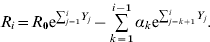
Note that R i corresponds to the available wealth at time i before withdrawal of the amount αi.
In the following sections, we will need the distribution function of random variables R i. For each i>0, R i is a sum of dependent log-normal random variables, which makes it impossible to determine its distribution function analytically. Therefore, we will use approximations. Several approximation techniques have been proposed throughout the literature, see e.g., Asmussen and Rojas (Reference Asmussen and Royas-Nandayapa2005), Dufresne (Reference Dufresne2004b), Milevsky and Posner (Reference Milevsky and Posner1998a) and Milevsky and Robinson (Reference Milevsky and Robinson2000). In this paper, we will use convex lower bound approximations based on comonotonicity, as proposed in Kaas et al. (Reference Kaas, Dhaene and Goovaerts2000) and Dhaene et al. (Reference Dhaene, Denuit, Goovaerts, Kaas and Vyncke2002a, Reference Dhaene, Denuit, Goovaerts, Kaas and Vynckeb). See also Huang et al. (Reference Huang, Milevsky and Wang2004) or Vanduffel et al. (Reference Vanduffel, Hoedemakers and Dhaene2005) for a comparison of some approximation techniques. In Section 4 a brief description is given of these comonotonic approximations. Since these results are analytical, we avoid simulation and hence reduce the computing effort drastically.
3.2 Mortality table
Throughout this paper we illustrate results using the Standard Ultimate Survival Model as proposed in Dickson et al. (Reference Dickson, Hardy and Waters2009). This mortality model follows Makeham's law, which means that the force of mortality, μx, is modeled as

where A>0, B>0 and c>1. Hence the force-of-mortality is assumed to consist of a positive constant and a term that increases exponentially with age. The constant term refers to age-independent causes of death, whereas the exponentially growing term describes the increasing mortality caused by aging. The probabilities of survival for this law are given by
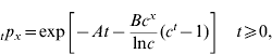
where tp x is the probability that an x-year old will survive for t years. We denote the probability that an x-year old will die within t years as tq x. Obviously it holds that tp x=1−tq x. Throughout this paper we will work in a discrete setting, with time intervals of 1 year.
In the Standard Ultimate Survival Model of Dickson et al. (Reference Dickson, Hardy and Waters2009) the following constants are used in (2): A=22×10−5, B=2.7×10⁻⁶ and c=1.124.
The ultimate age ω of the yearly life table is defined as the nonnegative integer that satisfies q ω−1=1q ω−1=1. In our examples we take ω=120.
Throughout this paper we assume that biometrical and financial risks are mutually independent; the return process of our investments is not influenced by lower or higher mortality and vice versa.
4 Comonotonic approximations
In this section we briefly describe the approximations we use to approximate the distribution function of the random variables R i as defined by (1). For more detailed information we refer to Dhaene et al. (Reference Dhaene, Denuit, Goovaerts, Kaas and Vyncke2002a, Reference Dhaene, Denuit, Goovaerts, Kaas and Vynckeb) and Dhaene et al. (Reference Dhaene, Vanduffel, Goovaerts, Kaas and Vyncke2005). Throughout this paper, we use the same notation and terminology as were used in the latter paper.
From Dhaene et al. (Reference Dhaene, Vanduffel, Goovaerts, Kaas and Vyncke2005) we know that

with S i being the stochastically discounted value of all future payments until time i:
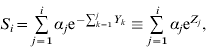
with 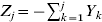 . As proposed in Kaas et al. (Reference Kaas, Dhaene and Goovaerts2000), we will use a comonotonic lower bound to approximate S i, which we denote as S il. This approximation is a conditional expected value: S il=E[S i|Λi]. For each random variable Λi, S il is a lower bound for S i in the convex order sense:

According to the definition of convex order, this means that E[S i]=E[S il] and that S i has higher stop-loss premiums than S il: E[(S i−d)+]⩾E[(S il−d)+] for all  . The conditioning random variable Λi is typically chosen as a linear combination of the yearly returns Y j. Assuming that
 , S il is given by

with U uniformly distributed on the unit interval and r ij being the correlation between Λi and Z j. If all coefficients, r ij, are positive, the terms in the sum S il are non-decreasing functions of the same random variable U and hence form a comonotonic random vector. In this case we call S il the comonotonic lower bound. The main advantage of this comonotonic dependency structure is that any distortion risk measure applied to such a comonotonic sum equals the sum of the risk measures of the marginals involved, see, e.g., Dhaene et al. (Reference Dhaene, Vanduffel, Tang, Goovaerts, Kaas and Vyncke2006). This property makes it straightforward to determine the distribution function of our approximation.
As explained in Dhaene et al. (Reference Dhaene, Vanduffel, Goovaerts, Kaas and Vyncke2005), maximizing (an appropriate approximation of) the variance of S il leads to the optimal  , with coefficients λij given by
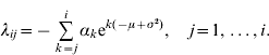
If the variables Y k are i.i.d., for k=1, …, i, the correlation coefficients r ij are given by
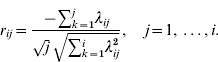
Using the optimal λij, coefficients (8) are non-negative, which means that (6) is a comonotonic sum. Hence, because of the aforementioned additivity property of comonotonic risks, the quantiles of (6) are given by

Using (9) we can easily determine the distribution function of S il. As is illustrated in Dhaene et al. (Reference Dhaene, Vanduffel, Goovaerts, Kaas and Vyncke2005) and Vanduffel et al. (Reference Vanduffel, Hoedemakers and Dhaene2005), using these results leads to an extremely accurate approximation of (the distribution function of) S i.
As explained in Dhaene et al. (Reference Dhaene, Vanduffel, Goovaerts, Kaas and Vyncke2005), the random variable S il is obtained from S i by changing the marginal distributions of the discount factors Z j in (4) and replacing the copula describing the dependency structure of the vector (Z 1, …, Z i) by the comonotonic copula. Important to note is that, when using a comonotonic lower bound, it is not the original marginals Z j that are assumed to be comonotonic but the transformed marginals. The concept of comonotinicity is therefore used only to obtain an accurate approximation of which the distribution function can easily be determined. Assuming that the cumulative returns or discount factors itself are comonotonic, which is not realistic, this is what is done when using the so-called comonotonic upper bound, see Kaas et al. (Reference Kaas, Dhaene and Goovaerts2000). Since the upper bound approximation is in general not very accurate, we do not use it here.
As a final step, we propose to approximate R i by R il, of which the distribution function is given by
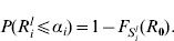
In the following section we will use (10) to approximate (3).
5 Lifetime ruin
5.1 Problem description
Recall that the available wealth on the account of the retiree at time i is given by R i, as defined by (1). Lifetime ruin occurs at a certain time j if the retiree is still alive at that time and if R j<αj, which means that the available wealth is not sufficient to make the desired withdrawal αj.
The moment of ruin, N, which is a random variable, is the first moment in time, n, when the available assets, R n, are less than the desired consumption, αn:
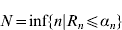
Note that N is a discrete random variable, since in our setting ruin can only occur at these discrete times where a withdrawal is made.
The probability that the retiree outlives his money, or the probability of lifetime ruin, is
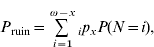
where ip x denotes the probability that an x-year old individual is still alive at age x+i and ω is the ultimate age of the life table. Our definition of the probability of lifetime ruin corresponds to the definition given by Milevsky et al. (Reference Milevsky, Ho and Robinson1997).
A retiree obviously wants his lifetime ruin probability to be as low as possible. In Section 8.2 we will discuss as to how the probability of lifetime ruin can be minimized in a framework of optimal portfolio selection.
To determine a value of P ruin, we need the distribution function of N, which can be determined using the following result.
Theorem 1.
The distribution of N is given by

and

Proof.
It is trivial that P(N=1)=P(R 1⩽α1). For i⩾2, we find that

The cash-flows αj are positive for all j, which means that recovery from ruin is not possible. Therefore, the event R 1>α1∩…∩R i−1>αi−1 is equivalent to R i−1>αi−1. Using this, we get
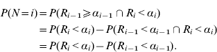
The last equality follows again from the fact that recovery from ruin is not possible. ▪
Using Theorem 1, we can rewrite the probability of lifetime ruin (11) as

where q x+i=1−p x+i is the probability that a person of age x+i will die within 1 year.
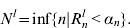
To determine P ruin we need the distribution function of the random variables R i, for all i>0. As seen in Section 4, we can, for each i, accurately approximate the available wealth R i by the comonotonic lower bound R il. Next, we approximate the moment of ruin N by N l:
Finally, we find an approximate value P ruinl for the probability of lifetime ruin P ruin:

In Section 8, a brief explanation is given of how our results can be translated into a framework of optimal portfolio selection.
5.2 Example
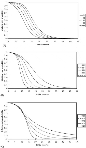
Suppose a retiree wants to withdraw a constant yearly amount of 1, or αi=1 for all i⩾1. Assume mortality is modeled by the Standard Ultimate Survival Model, as described in Section 3.2. In Figure 1, the lifetime ruin probability is depicted for a range of initial wealths R 0. Figure 1(A) gives the results for different retirement ages between 55 and 75, with given μ=0.05 and σ=0.10. We can see that increasing the retirement age leads to lower lifetime ruin probabilities; if consumption starts at an older age, the probability that a given R 0 is sufficient will clearly be higher.
(A) Probability of lifetime ruin (μ=0.05, σ=0.1, retirement age ∊(55,75)). (B) Probability of lifetime ruin (μ∊(0.02, 0.10), σ=0.1, retirement age=65). (C) Probability of lifetime ruin (μ=0.05, σ∊(0.05, 0.25), retirement age=65)

In Figure 1(B) the retirement age is fixed at 65, and σ=0.10. Results are given for different values of μ. We can see that an increase in the drift of the return process leads to a decrease in the lifetime ruin probability. Finally, Figure 1(C) shows the lifetime ruin probability for different values of σ, with μ=0.05 and the retirement age equal to 65. We see that if the initial wealth R 0 is large enough, higher volatility leads to a higher ruin probability. For small values of R 0, the opposite holds: higher volatility leads to a slightly lower ruin probability.
5.3 Accuracy of analytical approximations
In this paragraph we use a numerical example to illustrate the accuracy of our approximation for the probability of lifetime ruin, as described in Section 5.1. For more general information on the accuracy of convex order approximations based on comonotonicity, and in particular the convex lower bound approximation (6), we refer to Dhaene et al. (Reference Dhaene, Vanduffel, Goovaerts, Kaas and Vyncke2005).
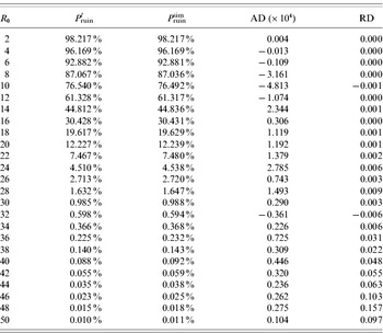
Assume a retiree aged 65, who withdraws a constant yearly amount of 1 (αi=1 for all i⩾1) and invests his wealth in an investment portfolio with drift μ=0.05 and standard deviation σ=0.10. In Table 1, the probability of lifetime ruin is computed for initial wealths R 0 between 2 and 50. For each value of R 0, P ruinl corresponds to the probability of lifetime ruin obtained using the analytical approximation (13), whereas P ruinsim is obtained through Monte Carlo simulation. This simulation was performed by generating 1,000×10,000 sample paths. Note that this simulation, and simulation in general, is much more time-consuming compared to our analytical approximations. In the table, the absolute difference (AD) and relative difference (RD) between the different methods are given. The latter is determined as  .
Probability of lifetime ruin: comparison between analytical approximation and simulation (μ=0.05, σ=0.1, retirement age=65)

The results in Table 1 clearly show that our convex order approximations are very accurate.
6 Conditional time of lifetime ruin
In the previous section we have seen how we can accurately approximate the probability of lifetime ruin. However, only looking at the probability of lifetime ruin can give an incomplete view, and can be misleading. For a retiree, it is not only important to know how likely he is to experience financial ruin before he dies. A second concept that can be useful is the time of ruin: if ruin occurs, if a retiree runs out of money while he is alive, when is it most likely to take place?
Denote the moment of lifetime ruin by T. This means that P ruin=Pr(T<∞). The conditional probability that lifetime ruin happens at time j, given that ruin occurs, is equal to

Similarly, the conditional probability that ruin occurs before or at time j equals

To determine the distribution function of this conditional time of lifetime ruin we use the lower bound approximations of Section 4. We denote the approximated time of lifetime ruin by T l.
The following example shows that restricting attention to the probability of lifetime ruin can give an incomplete view.
6.1 Example
Suppose a 65-year old retiree has an initial wealth R 0=20 and suppose that he wants to withdraw an amount of 1 every year; αi=1 for all i. In other words, the retiree has a spending rate r equal to 5%. If he invests his wealth according to a conservative strategy with drift μ=0.025 and standard deviation σ=0.01, the retiree has a lifetime ruin probability P ruinl of 27.72%. If he invests more aggressively, with μ=0.045 and σ=0.15, his ruin probability is almost the same: P ruinl of 27.75%. Based on this, the retiree is indecisive between the two strategies, as the difference in ruin probability is negligible.
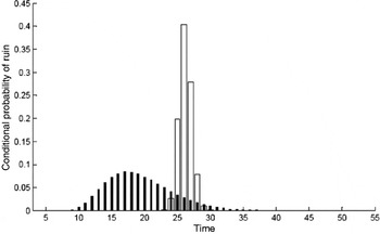
However, the conditional time of ruin is significantly different, as can be seen from Figure 2. White bars depict the conservative investment strategy, black bars depict the more aggressive one. The retiree will clearly prefer the first strategy, as ruin is likely to occur significantly later. If the unlikely event of ruin occurs, it is very unlikely to happen before the retiree reaches the age of 90 in the first case. In the second case, if ruin occurs, it will most likely (almost 90% probability) occur before he reaches age 90. The expected value and standard deviation of the conditional time of ruin equal, respectively, 20.30 and 5.29 in the first case and 28.52 and 1.18 in the second case.
Conditional time of ruin: conservative strategy (white bars) versus aggressive strategy (black bars), with comparable lifetime ruin probability

7 Wealth at death
In previous sections, we have discussed lifetime ruin and the conditional time of ruin. A related concept a retiree might be interested in is that of knowing how much wealth he will leave to his heirs at his death. The bequest or wealth at time of death, denoted by B, is a random variable, from which we will determine the distribution function in this section. Given that the retiree dies in the period (i−1, i), which happens with the probability i−1p xq x+i−1, the bequest B corresponds to R i, which is the available wealth at time i. Therefore we have for any b:

In practice, we are only interested in positive values of b.
Note that the probability of lifetime ruin as defined by (11) corresponds to the probability of having a bequest smaller than or equal to zero:
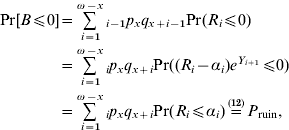
where the second equality follows because Pr(R 1⩽0)=0.
To determine the distribution function of the bequest B we use the lower bound approximations described in Section 4. Denoting the approximated bequest by B l, we get

As an alternative, we can also look at the distribution of the conditional bequest, conditioned on the event that lifetime ruin does not occur. It can easily be seen that, for any b⩾0,

and

Again, we can use our comonotonic approximations to compute (14) and (15).
7.1 Example
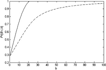
Consider the same setting as in the example in Section 6.1. We have seen that the two strategies described in Section 6.1 lead to (approximately) the same lifetime ruin probability. Based on the distribution of the conditional time of lifetime ruin, the retiree prefers the more conservative strategy. However, looking at the distribution of the bequest leads to the opposite conclusion, as can be seen clearly from Figure 3. The probability of leaving a positive wealth at death is significantly higher for the more aggressive strategy. For example, for the conservative strategy, the probability of leaving more than 20 is equal to zero, whereas this is more or less 30% for the more aggressive strategy. Note that, as explained above, the intersection of the distribution function with zero corresponds to the lifetime ruin probability, which, indeed, is more or less equal for both strategies.
Distribution of bequest: conservative strategy (full line) versus aggressive strategy (dashed line), with comparable lifetime ruin probability

We come to the same conclusion by, e.g., comparing the expected value and standard deviation of the conditional bequest. For the conservative strategy, we find that the expected conditional bequest equals 8.45, with a standard deviation of 5.37. For the aggressive strategy, both values are significantly higher: an expected value of 25.85, with a standard deviation of 27.77.
8 Optimal portfolio selection problems
8.1 Framework and notation
Optimal portfolio selection corresponds to finding the best allocation of the available wealth in a basket of risky or risk-free assets or asset classes. In this paper we work with so-called constant mix strategies: the investment proportions are kept constant by continuously rebalancing the assets. At each time instant, assets have to be bought or sold, to keep the asset mix at the initial level. In Dhaene et al. (Reference Dhaene, Vanduffel, Goovaerts, Kaas and Vyncke2005) optimal portfolio selection problems in a provisioning and saving context are discussed using the same setting.
As explained in Section 5, we work in a lognormal setting. We assume the classical multi-period, continuous-time framework of Merton (Reference Merton1971), also known as the Black and Scholes (Reference Black and Scholes1973) setting. See e.g., Björk (Reference Björk1998) for more details on this setting. When the portfolio is continuously rebalanced such that the investment proportions are kept constant, it can be shown that the portfolio return is also lognormally distributed. This was derived in Merton (Reference Merton1971, Reference Merton1990), see also Rubinstein (Reference Rubinstein1991), using stochastic arguments and Itô's Lemma. Milevsky and Posner (Reference Milevsky and Posner1998b) derived the same result using more elementary arguments, by taking limits of lognormal sums.
We assume there are m risky assets or asset classes available in the market. In our examples, we assume there is no risk-free asset class available. An investment portfolio is described by a vector πT=(π1, …, πm), where πt is the proportion invested in risky asset i. Obviously it must hold that  . Although our results also hold in the general case, we assume short-selling is not allowed, which means 0⩽πi⩽1.
Investing an amount of 1 at time k−1 in asset i will grow to  at time k. The return in a given year k is assumed to be independent of the return in any year, l≠k:

In a given year k, however, the returns of the different asset classes are correlated:

We use the notation σi2=σii.
For a fixed asset i, the random variables Y ki, k⩾1, are assumed i.i.d., normally distributed with mean  and variance σi2. The drift vector and variance-covariance matrix of the risky assets are denoted by μT=(μ1, …, μm) and Σ respectively, with (Σ)i,j≡σij. Note that Σ has to be positive-semidefinite, which means that xT·Σ·x⩾0 for all m-dimensional vectors x.
The drift vector and volatility corresponding to an investment portfolio π are written as μ(π) and σ2(π). We find that

The yearly returns, Y i(π), of an investment portfolio π, are independent and normally distributed random variables, with expected values E[Y i(π)]=μ(π)− and variance Var[Y i(π)]=σ2(π).
To use the random variables introduced in Section 4 in our optimal portfolio selection setting, we make them dependent on an investment portfolio π by adapting the notation; we use, e.g., R i(π), S il(π) and P ruin(π).
8.2 Minimizing lifetime ruin probability
8.2.1 Problem description
As a first optimization problem, we consider the following:

We want to find the strategy that minimizes the probability that the retiree outlives his money. We denote the optimal strategy by π* and the corresponding minimal probability of lifetime ruin by P*.
Using classical Markowitz mean-variance analysis, we can reduce this optimization problem (17) to a one-dimensional optimization. Consider two portfolios, π1 and π2, with σ(π1)=σ(π2) and μ(π1)<μ(π2). As is discussed in Dhaene et al. (Reference Dhaene, Vanduffel, Goovaerts, Kaas and Vyncke2005), we find that

which means that

Hence, using (12) we get
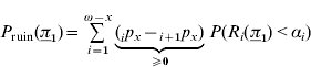

This means that for each σ we only have to consider the corresponding portfolio with maximal drift, which we denote by
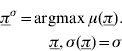
Optimization problem (17) can therefore be reduced to
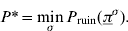
Finally, we approximately solve optimization problem (17) using results from Section 4:

The resulting optimal investment portfolio is denoted by πl.
8.2.2 Numerical example
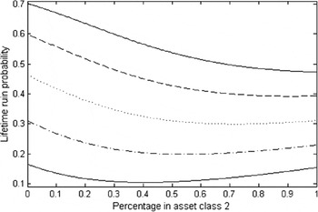
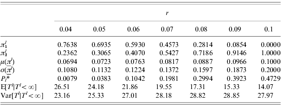
Suppose we have two risky asset classes available in which we can invest, with drift vector μT=(0.06, 0.10), standard deviations σT=(0.10, 0.20) and correlation ρ1,2=0.50. Suppose a 65-year old retiree wants to withdraw a constant amount per year, expressed as a percentage r of his initial wealth: αi=rR 0 for all i. Solving optimization problem (20) in this setting leads to the following results. In Table 2, the optimal strategies and their corresponding minimal lifetime ruin probabilities  are given in terms of a range of spending rates r. We see for example that if the retiree wants to spend 5% of his initial wealth per year, he should invest according to the strategy (0.6935, 0.3065), with corresponding drift 0.0723 and standard deviation 0.1132. This leads to a lifetime ruin probability of 3.83%. If he would invest his wealth according to a different strategy, the ruin probability associated with the spending rate of 5% would be higher. From the results we can see that width increasing r the minimal lifetime ruin probability increases, and that the retiree has to invest increasingly aggressively (more in the second asset class) to realize this minimal ruin probability. Figure 4 illustrates the optimization problem graphically.
Lifetime ruin probability for spending rate x (upper full line: x=0.1, dashed line: x=0.09, dotted line: x=0.08, dash-dotted line: x=0.07, lower full line: x=0.06)

Optimal strategy leading to minimal lifetime ruin probability for range of spending rates, with retirement age 65
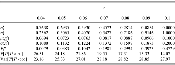
In Table 2, the expected value and the variance of the conditional time of ruin are also given for the optimal strategies. We can see that an increase in the spending rate r leads not only to higher lifetime ruin probabilities but also to lower conditional expected times of ruin. This indicates that, even if the optimal investment strategy is followed, the more a retiree spends, the more likely he is to experience financial ruin and, moreover, the earlier this ruin is likely to happen.
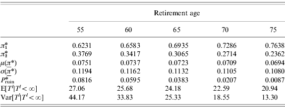
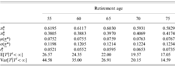
In Table 3 optimization problem (20) is solved for a range of retirement ages. The spending rate r is chosen to be equal to 0.05. We see that a higher retirement age leads to a lower minimal lifetime ruin probability. Retiring at a higher age also means the retiree has to follow a more conservative strategy to obtain his minimal lifetime ruin probability.
Optimal strategy leading to minimal lifetime ruin probability for range of retirement ages, with spending rate equal to 0.05
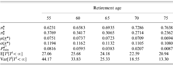
Adding the retirement age to the expected conditional time of ruin, we see from Table 3 that, given that ruin occurs, the expected age at the moment of lifetime ruin increases with an increasing retirement age.
8.3 Maximizing sustainable spending rate
8.3.1 Problem description
As a second optimization problem we maximize the sustainable spending rate. Although a retiree wants the highest spending rate possible, he also wants to sustain his spending throughout his retirement years. Incorporating a predetermined lifetime ruin probability ε, we determine the investment strategy π leading to a maximal spending rate r. Recalling that αi=rR 0 for all i, we can rewrite P ruin(π) as

which is increasing in r. Assuming a ruin probability ε, we denote, for each investment strategy π the spending rate is such that P ruin(π)=ε as r(π). Denoting the maximal spending rate by r*, we get the following optimization problem:

Following reasoning similar to that in Section 8.2, we can show that (21) is equivalent to the following one-dimensional optimization problem:
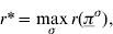
with πσ given by (18). As in Section 8.2 we use the comonotonic lower bound approximations to find an approximation for r*, which we will denote by  . We denote the strategy leading to this maximal spending rate by πl.
8.3.2 Numerical example
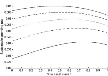
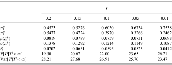
As in Section 8.2.2, suppose we have two risky asset classes available in which we can invest, with drift vector μT=(0.06, 0.10), standard deviations σT=(0.10, 0.20) and correlation ρ1,2=0.50. Suppose a 65-year old retiree wants to withdraw each year a percentage r of his initial wealth: αt=rR 0 for all i. In Table 4, the optimal investment strategies and corresponding maximal sustainable spending rates r l* are given for a range of lifetime ruin probabilities ε. For example, if we consider a lifetime ruin probability of 10%, we see that the retiree can, each year, withdraw 5.95% of his initial wealth if he invests according to the strategy (0.6030, 0.3970). If he invests according to a different strategy, the sustainable spending rate will be lower than 5.95%. From these results we see that decreasing the lifetime ruin probability decreases the maximal sustainable spending rate and leads to a more conservative optimal investment strategy. Investing more conservatively also leads to respectively a higher expected value and lower variance of the conditional time of ruin. Figure 5 illustrates the optimization problem graphically.
Sustainable consumption for given lifetime ruin probabilities P ruin (upper full line: P ruin=0.20, dashed line: P ruin=0.15, dotted line: P ruin=0.10, dash-dotted line: P ruin=0.05, lower full line: P ruin=0.01)

Optimal strategy leading to maximal sustainable withdrawal for range of lifetime ruin probabilities, with retirement age 65
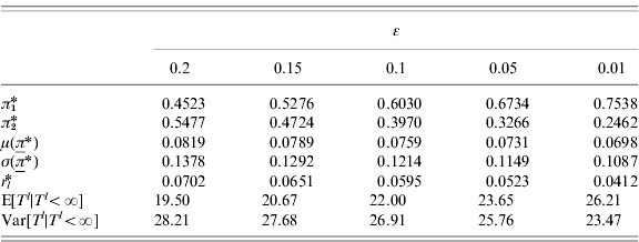
In Table 5, optimization problem (21) is solved for a range of retirement ages. The lifetime ruin probability ε is taken to be equal to 0.10. We see that increasing the retirement age increases the maximal sustainable spending rate. In this example the retirement age only slightly influences the optimal investment strategy.
Optimal strategy leading to maximal sustainable spending rate for range of retirement ages, with lifetime ruin probability equal to 0.10
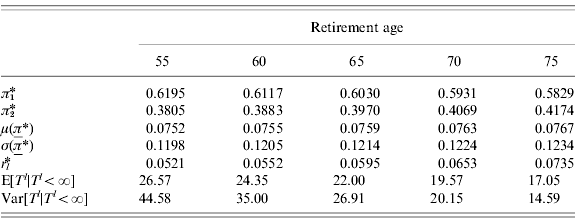
Adding the retirement age to the expected conditional time of ruin, we see that, given that ruin occurs, the expected age at the moment of lifetime ruin increases with increasing retirement age.
8.4 Maximizing conditional expected time of lifetime ruin
As a third optimization problem, we maximize the expected conditional time of ruin, as described in Section 6. Again, we solve this problem using the comonotonic approximations defined in Section 4. The maximal expected conditional time of lifetime ruin ET l is given by

Considering two portfolios with the same standard deviation, σ, the portfolio with the highest drift μ unfortunately does not necessarily result in the highest conditional expected time of lifetime ruin. Therefore, unlike the optimization problems in the previous sections, (22) can, in general, not be reduced to a one-dimensional optimization problem, which makes solving (22) much more time-consuming.
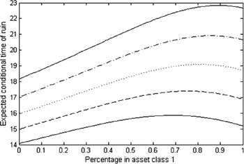
Expected conditional time of ruin for spending rate x (lower full line: x=0.1, dashed line: x=0.09, dotted line: x=0.08, dash-dotted line: x=0.07, upper full line: x=0.06)

8.4.1 Numerical example
As in Section 8.2.2, suppose we have two risky asset classes available in which we can invest, with drift vector μT=(0.06, 0.10), standard deviations σT=(0.10, 0.20) and correlation ρ1,2=0.50. As mentioned above, (22) can, in general, not be reduced to a one-dimensional optimization. However, since we only have two asset classes, fixing a value for σ also fixes μ, which means (22) is reduced to a one-dimensional problem in this case.
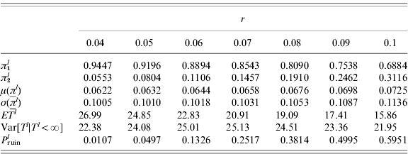
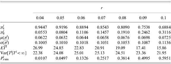
Suppose a 65-year old retiree wants to withdraw, each year, a percentage r of his initial wealth: αi=rR 0 for all i. In Table 6, the optimal investment strategies and corresponding maximized conditional expected times of ruin are given for a range of spending rates r. We see the same dynamics as in Table 2: increasing the spending rate leads to a more aggressive optimal strategy. We also see that the resulting maximized expected conditional times of ruin decrease with increasing spending rates, whereas probabilities of lifetime ruin increase. Hence, increasing the desired spending rate implies an increasing probability of financial ruin, and moreover, if ruin happens, it is likely to happen at an earlier age. Figure 6 illustrates the optimization problem graphically.
Optimal strategy leading to maximal expected conditional time of ruin for range of spending rates
9 Conclusion
In this paper, we started by discussing the concept of lifetime ruin. From the point of view of an individual retiree, we defined lifetime ruin as running out of money while being alive. In a multivariate lognormal setting, we investigated the probability of lifetime ruin and the determination of a sustainable spending rate. In relation to this concept, we discussed the conditional time of lifetime ruin and the notion of bequest or wealth at death. Using an intuitive numerical example, we illustrated that making investment decisions is not always straightforward. Depending on the criterion used, a retiree might have different investment preferences. Our example indicates that a retiree should always make well-considered decisions, balancing between the most relevant criteria.
In the last part of our paper we have discussed several optimal portfolio selection problems. We explained how to minimize the probability of lifetime ruin, maximize the sustainable spending rate and maximize the conditional expected time of lifetime ruin. Each of these optimization problems is illustrated with intuitive numerical examples. By solving these general optimization problems, we believe that our results provide a valuable tool, helping retirees to make conscious investment decisions.
As pointed out in Section 2, the problems discussed in this paper have been examined in earlier research papers. Our paper provides a new approach to solving problems related to the probability of lifetime ruin, using analytical approximations based on the concept of comonotonicity. Our paper is an addition to existing literature primarily because we take the random lifetime of the retiree into account when considering lifetime ruin, as well as its related problems. As explained in the introduction, few papers in the current literature have followed this realistic approach. Often a fixed moment of death is assumed, or results are restricted to the assumption of a constant force of mortality. As shown for a related problem in Milevsky et al. (Reference Milevsky, Moore and Young2005), the shape of the force of mortality has a significant impact on optimal investment strategies, which means that the assumption of a constant force of mortality is unrealistic. Second, our analytical approach allows to solve more general optimal portfolio selection problems compared to earlier studies. Typically, optimization problems such as those discussed in our paper are solved using Monte Carlo simulation. Since this is generally very time-consuming, a trade-off often has to be made between speed and accuracy. Moreover, using simulation, it is hard to obtain results for the whole range of admissible investment portfolios, meaning that the analysis is usually restricted to a subset of the admissible portfolios. Also, determining the optimal portfolio when more than two asset classes are available can become too cumbersome when using simulation. Our approach allows to consider a higher number of asset classes without significantly increasing the computational complexity. In our paper we avoid simulation using analytical approximations based on comonotonicity. The analytical nature of our expressions means that they can be computed very quickly. Furthermore, we have seen that our approximations are highly accurate. Using our approach, a decision-maker can quickly acquire a complete picture of the different aspects that might influence his investment decisions.
Also, contrary to a large part of the existing literature, our approach allows us to work in a discrete-time setting, and to assume that the retiree consumes his wealth at discrete points in time. This is, in our opinion, more realistic and more intuitive to understand than assuming a continuous consumption rate.
Further research could consists in generalizing our results allowing for the consumption scheme to be stochastic or in extending our results to more general return processes, e.g., to a Lévy-type or elliptical-type setting. Bounds and approximations for sums of random variables with distributions of this type are considered in Albrecher et al. (Reference Albrecher, Dhaene, Goovaerts and Schoutens2005) and Valdez et al. (Reference Valdez, Dhaene, Maj and Vanduffel2009). Another possible extension is to use a projected life table to model mortality, modeling future survival probabilities as random variables. To conclude, future work could also include generalizing our results to multiple life states, where individual lives can be mutually dependent.