1. Introduction
This paper describes the work done so far in the field of the delta catching system. The work involves selecting the catching system, kinematic synthesis of delta manipulator, the design of components, dynamics analysis of the system, and control analysis.
Boney [Reference Bonev1] has explained the story of the success of the delta parallel robot. Robots achieve acceleration up to 50g in experiments and 12g in industrial use. Delta robot is perfect for application where the light object must be placed from one place to another (10 g to 1 kg).
Murray [Reference Zsombor-Murray2] has discussed the kinematic analysis of the delta robot (Clavel’s) by the geometric method. The geometric configuration of Clavel’s delta manipulator is explained in detail. Tsai [Reference Tsai3] has discussed the position analysis of the University of Maryland manipulator. The manipulator’s graphical and algebraic solutions for direct and inverse kinematic analysis have been explained. Codourey [Reference Alain4] has demonstrated the dynamic modelling of robots (parallel) estimated torque control implementation. The number of forces and motion of the end effector is significantly less in the concept of micromanipulation.
Laribi [Reference Laribi, Romdhane, Zeghlou and l5] has explained the dimensional analysis of the delta robot for a specified workspace, i.e., designs a dimensional configuration of a delta manipulator for a given workspace. Kosinska [Reference Kosinska, Galicki and Kedzior6] has explained the optimization of variables of the delta robot for a workspace. This paper has presented the methodology of deriving design constraints from the closed-loop configuration of the delta-4 parallel manipulator. The initial conceptual design has been taken from Clavel’s delta configuration.
Tsai [Reference Tsai7] has explained the methodology based on the principle of virtual work for static analysis of parallel robots.
The dynamic analyses of the multibody system are required to know the trajectory of the different coordinates for a given torque or for a required trajectory what should be the torque at another degree of freedom. There are various methods available for the formulation of the multibody system. Angeles and Lee [Reference Angeles and Ma8] developed and implemented a computationally efficient and systematic algorithm for formulating the dynamic model of a constrained mechanical system. The dynamic equations of a mechanical system composed of rigid bodies coupled by holonomic constraints are derived using an orthogonal complement of the matrix of the velocity constraint equations. The kinematic constraints are expressed as a system of dependent homogeneous linear equations on the twist of the different rigid bodies. Angeles and Ma [Reference Angeles and Lee9] used the concept of natural orthogonal complement used in the derivation of an
 $ n\times n$
inertia matrix of an
 $ n$
-axis manipulator. The two methods are presented to compute the joint acceleration through the governing equation of motion. The first method is based on the Cholesky decomposition of the inertia matrix. The second method is based on a composition of the minimum norm and least square approximation of under-determined and over-determined linear algebraic systems, respectively.
Saha [Reference Saha10] states that inertia matrix manipulator decomposition is necessary. The joint accelerations are computed through the equations of motion. The recursive relations between the elements of the computed matrices reveal through the Gaussian elimination of the inertia matrix. Saha [Reference Saha11] has derived restricted dynamic equations of motion for the serial multibody systems. It has rigid bodies in the serial kinematic chain. The Euler–Lagrange independent equation of motion has been calculated. The Newton–Euler equations of motion of uncoupled bodies were used to obtain a recursive inverse and forward dynamic algorithm required to control and simulate the mechanical system. Saha [Reference Saha12] explained the method of recursive dynamics algorithms for multibody systems with serial, parallel, and closed-loop chains using the concept of decoupled natural orthogonal complement. The definition of the NOC and DeNOC and features of the DeNOC matrices are presented. The method illustrated forward and inverse dynamics with several multibody systems, e.g., a parallel manipulator and six DOF serial manipulators.
The DeNOC matrices can be written recursively for the number of links of a multibody system. The DeNOC method provides the equation of motion in terms of the joint angle, the same as the Euler-Lagrange formulation (energy-based approach). In this formulation, Newton–Euler (linear and angular) equation of motion is transferred to angular only (in terms of joint angles). This method reduced the large set of the equation to a minimal set of the equation by converting the equation of motion in terms of joint angle only, e.g., for one link Newton–Euler gives two equations of motion, while using the DeNOC, it is converted to only one equation of motion [Reference Saha13].
2. Robots for Catching
Through the years, researchers and engineers have developed various catching-based robots [Reference Shinno, Yoshioka and Sawano14–Reference McBean and Breazeal18]. Major catching-based robotic systems were developed in the mid-1990s and 2000s. Philip W. Smith et al. [Reference Philip, Nandha Kumar and Ramadorai19] proposed vision-based robust robotic catching algorithms that are used for objects having non-rigid in nature. It is based on an image-based representation of the non-rigid structure and relative elasticity with no a priori physical model. The relative elasticity has many advantages as simplicity, comprehensiveness, generality. This method overcomes many limitations of existing non-rigid object catching.
Satoshi Yonemoto et al. [Reference Yonemoto and Taniguchi20] proposed mapping real-time human action with its corresponding virtual environment. In this approach, the scene constraints fall between the user motion and the virtual object. This approach has resulted in the action information and non-trivial to have the body postures representation. Yejun Wei et al. [Reference Wei and Goodwine21] described non-smooth domains and demonstrated and verified a motion planning algorithm for the system. This approach performs catching on a non-smooth object using four fingers. Park et al. [Reference Park and Ayanna22] described a method that takes the visual data to produce force guidance data and an applicable tele-manipulative system. Mkhitaryan et al. [Reference Mkhitaryan and Burschka23] presented a vision-based haptic multisensory. The system interacts with objects of having fragile nature. Chen et al. [Reference Chen, Zhang, Zhang and Kwok24] revealed the significance of active lighting control in the domain of robotic catching. Kansal et al. [Reference Sachin and Sudipto25] proposes the vision-based kinematics analysis of the delta robot for object catching.
In this paper, robot catching application presented introduces a new robot application domain. A new manipulative parallel robot system is developed, entailing the design and analysis of a new system. In Section 2 (A), the proposed methodology has been discussed. Section 2 (B) discusses mechanical structure design. In Section 3, kinematic analysis and experimental setup used is discussed. In Section 4, dynamic analysis is discussed. In Section 5 catching the object is examined. Results and validation are discussed in Section 6.
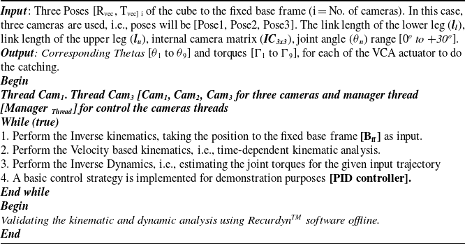
Extracting the pose of the cube, i.e., (three translations and three rotations and it come out to be 6-DOF) with respect to the fixed base coordinates system using the camera as a vision sensor. After that, inverse kinematics is executed for all three delta robots. The thetas (θ1 to θ9) from the three delta robots feeding the calculated thetas to the controller of the manipulating system is executed. Getting feedback from the encoder and PID control scheme is also implemented. The tuning of the PID values is achieved at every cycle using the optimizing technique (Genetic Algorithm). Dynamic analysis of the system using Decoupled Natural Orthogonal Complement (DeNOC) technique is applied; validation of the dynamic analysis results with the RecurdynTM software is also achieved. Validation of the kinematic analysis results with the RecurdynTM software is also completed. Knowing the torque v/s theta behaviour (both the directions) of the voice coil actuator (VCA), i.e., the actuator, the estimation of torque by giving the theta corresponding is also validated with the dynamic analysis results.

2.1. Proposed method
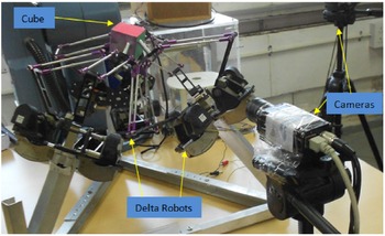
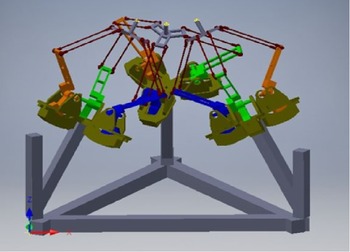
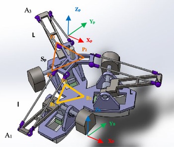
Three parallel robots are arranged in symmetrical order with vision sensors and hardware interfacing, as shown in Fig. 1. This paper is limited to the kinematic and dynamic analyses of the system to catch the cube. In this method, a new architecture that comprises of three delta robots and each of the end effectors behave like one finger, so it comprises three fingers that do the catching in the real-time scenario. Three pre-calibrated vision sensors (Basler scout cameras) are used to estimate the pose of the three cube faces. The forward kinematics for all three fixed delta robots is achieved to know the shared workspace (Wcatch = Intersection (W1, W2, W3)).
Experimental setup.

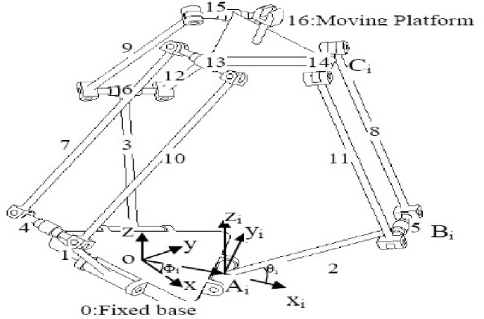
The delta robots are used as fingers because this architecture can go for a high payload and is dedicated to high-speed applications like manipulation. In this architecture, the moving frame has no rotation to the fixed frame, i.e., 3DOF has the only translation in the X, Y, Z axes, as shown in Fig. 2.
Mechanical structure of individual manipulator [Reference Sachin, Rajesh and Sudipto26].

2.2. Mechanical structure
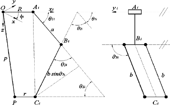
The delta robot is the three-DOF motion platform invented by a research team led by Prof. Reymond Clavel in the early 1980s as a manipulator for light and smaller objects. Since then, it has been used for various applications in industries and elsewhere. Their applications include driving simulators, medical devices, entertainment industries, vibration isolators, etc. Delta manipulator, as shown in Fig. 3, employs revolute joints and spherical joints to give platform output to translational motion [Reference Zsombor-Murray2]. A schematic diagram of the manipulator constructed with all revolute joints. The lower arm is labelled as links 1, 2, 3. The upper arms of the delta robot architecture comprise four parallelograms; links are shown in Fig. 2. Links 4, 7, 10, and 13 are marked as Ist limb, links 5, 8, 11, and 14 are marked as the IInd limb, and links 6, 9, 12, and 15 are marked as IIIrd limb.
Three delta combined system architecture [Reference Sachin and Sudipto27].

A, B, C are the points where three parallel joints attach the lower arms, upper arms, the two surfaces, and each of the parallelograms has four revolute joints. Overall, there are 17 links and 21 revolute joints. The general degree of freedom equation is
 \begin{align}n = \,\,s\,\left( {r\, - \,p\, - \,1} \right) + \Sigma \,{n_i}\end{align}
where S represents dimensions of working space (For spatial, s = 6), R represents several rigid bodies or links in the system = 17, and P represents nunmber of kinematic pairs of joints in the system = 21
n i = relative degree of freedom of each joint.
 \begin{align*}DOF,\,n = \, = \,6^{*}(17\, - \,21 - \, - \,1) + 21\left( 1 \right) = - 9\end{align*}
The joints are redundant and have a 3DOF translation. Due to the four-bar parallelogram and the three revolute joints at points A, B, and C, the limb constrains the unfixed surface from rotating about the z and x-axis. The two limbs constraint the unfixed body from rotating about any axis. It is helpful in the x-y-z positioning device.
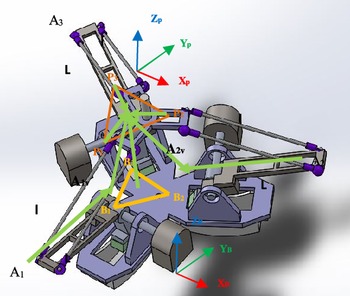
The delta manipulator used in this paper is shown in Fig. 4. The base platform was 0, and the top platform was 1, as shown in Fig. 4. The inclination of the second link due to a spherical joint cannot be shown in the X-Z plane. The angle between any two axes X, u1, v1 is 120 o, and the direction of axes Z, w1, and w2 is the same.
Schematic diagram of delta mechanism.

3. Kinematic Analysis
3.1. System description and mathematical background
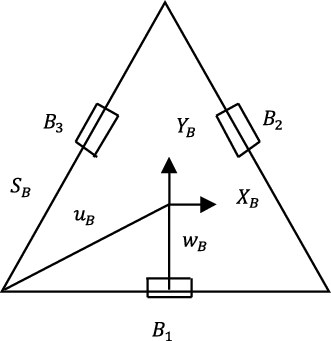
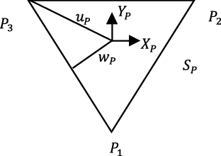
The three degrees of freedom delta robot is capable of 3D transitional of its moving surface. As in the proposed delta architecture, there are three identical Revolute-Universal-Universal (R-U-U) chains as legs. In the Figs. 5 and 6, points Bi, i = 1,2,3 are the hips, points, Pi, i = 1,2,3 are the ankles, and points, Ai, i = 1,2,3 are the knees. sB represents the length of the equilateral triangle (base), and sP represents the length of the equilateral triangle (moving). In our proposed delta architecture, the moving platform is inverted to the base. There is no rotation between the moving platform and the base platform, i.e., [R3x3 is Identity matrix]. Thus, only the translational vector between the moving and the fixed platform is to be considered.
Delta robot fixed base schematic.

Delta robot moving platform.

‘B’ represents the cartesian reference frame (fixed). The origin is situated in the centre of the bottom triangle.
 $\text{'}$
P’ is not a fixed Cartesian reference frame. The origin is located in the centre of the platform triangle. The rotation matrix
 $ \begin{array}{c}B\\ P\end{array}\textit{R}$
= I
3
always is constant as orientations of P and B are the same. The joint variables are θ = {θ1, θ2, θ3}T, and the Cartesian parameters are
 $ \begin{array}{c}B\\ P\end{array}\textit{R}$
= {x y z}T..The three upper legs of lengths
 $\text{'}$
L’ and three lower legs of lengths
 $\text{'}$
l’ have high symmetry. The geometric details of the delta robot having a fixed bottom and platform are depicted in Figs. 5 and 6, respectively.
In the bottom frame
 $\text{'}$
B
 $\text{'}$
, the fixed-bottom joint points Bi are constant. In the top frame
 $\text{'}$
P
 $\text{'}$
, the platform-fixed joint points Pi is constant. In the kinematic diagram (in Fig. 7), the three vector-loop closure equations for the parallel architecture are given below:
 \begin{align*} \begin{array}{c}B\\ \\[-7pt] 1\end{array}B&=\left\{\begin{array}{c}0\\ \\[-7pt] -{w}_{B}\\ \\[-7pt] 0\end{array}\right\} \textrm{}\textrm{}\textrm{}\textrm{}\textrm{}\textrm{}\textrm{}\textrm{}\textrm{}\textrm{}\textrm{}\textrm{}\textrm{}\textrm{}\textrm{}\textrm{}\begin{array}{c}B\\ \\[-7pt] 2\end{array}B=\left\{\begin{array}{c}\dfrac{\sqrt{3}}{2}{w}_{B}\\ \\[-7pt] \dfrac{1}{2}{w}_{B}\\ \\[-7pt] 0\end{array}\right\}\textrm{}\textrm{}\textrm{}\textrm{}\textrm{}\textrm{}\textrm{}\textrm{}\textrm{}\textrm{}\textrm{}\textrm{}\textrm{}\textrm{}\textrm{}\begin{array}{c}B\\ \\[-7pt] 3\end{array}B=\left\{\begin{array}{c}\dfrac{-\sqrt{3}}{2}{w}_{B}\\ \\[-7pt] \dfrac{1}{2}{w}_{B}\\ \\[-7pt] 0\end{array}\right\}\\ \\[-7pt]\begin{array}{c}p\\ \\[-7pt] 1\end{array}P&=\left\{\begin{array}{c}0\\ \\[-7pt] -{u}_{P}\\ \\[-7pt] 0\end{array}\right\} \textrm{}\textrm{}\textrm{}\textrm{}\textrm{}\textrm{}\textrm{}\textrm{}\textrm{}\textrm{}\textrm{}\textrm{}\textrm{}\textrm{}\textrm{}\textrm{}\textrm{}\textrm{}\textrm{}\textrm{}\begin{array}{c}p\\ \\[-7pt] 2\end{array}P=\left\{\begin{array}{c}\dfrac{{S}_{p}}{2}\\ \\[-7pt] {w}_{P}\\ \\[-7pt] 0\end{array}\right\}\textrm{}\textrm{}\textrm{}\textrm{}\textrm{}\textrm{}\textrm{}\textrm{}\textrm{}\textrm{}\textrm{}\textrm{}\textrm{}\textrm{}\textrm{} \textrm{}\begin{array}{c}p\\ 3\end{array}P = \left\{\begin{array}{c}\dfrac{-{S}_{p}}{2}\\ {w}_{p}\\ 0\end{array}\right\}\end{align*}
Delta robot kinematic diagram.

The vertices of the bottom triangle (fixed) are represented as
 \begin{align*} \begin{array}{c}B\\ \\[-7pt] 1\end{array}b=\left\{\begin{array}{c}\frac{{S}_{B}}{2}\\ \\[-7pt] -{w}_{B}\\ \\[-7pt] 0\end{array}\right\} \textrm{}\textrm{}\textrm{}\textrm{}\textrm{}\textrm{}\textrm{}\textrm{}\textrm{}\textrm{}\textrm{}\textrm{}\begin{array}{c}B\\ \\[-7pt] 1\end{array}b=\left\{\begin{array}{c}0\\ \\[-7pt] {u}_{B}\\ \\[-7pt] 0\end{array}\right\}\textrm{}\textrm{}\textrm{}\textrm{}\textrm{}\textrm{}\textrm{}\textrm{}\begin{array}{c}B\\ \\[-7pt] 3\end{array}b=\left\{\begin{array}{c}\frac{-{S}_{B}}{2}\\ \\[-7pt] {-w}_{B}\\ \\[-7pt] 0\end{array}\right\}\end{align*}
where:
 $ {w}_{B}=\frac{\sqrt{3}}{6}{S}_{B}$
;
 $ {w}_{p}=\frac{\sqrt{3}}{6}{S}_{p}$
;
 $ {u}_{B}=\frac{\sqrt{3}}{3}{S}_{B};\ {u}_{p}=\frac{\sqrt{3}}{3}{S}_{p}$
In the kinematic diagram, the three vector-loop equations as depicted in Fig. 7;
 \begin{align} &\left\{\begin{array}{c}B\\ i\end{array}B\right\}+\left\{\begin{array}{c}B\\ i\end{array}L\right\}+\left\{\begin{array}{c}B\\ i\end{array}l\right\}=\left\{\begin{array}{c}B\\ i\end{array}P\right\}+\left[\begin{array}{c}B\\ P\end{array}R\right]\left\{\begin{array}{c}P\\ i\end{array}P\right\}=\left\{\begin{array}{c}B\\ P\end{array}P\right\}+\left\{\begin{array}{c}P\\ i\end{array}P\right\}\textrm{}\textrm{}\textrm{}\textrm{}\textrm{}\textrm{}\nonumber\\[3pt] i &=\textrm{1,2},3\end{align}
 $ \left[\begin{array}{c}B\\ P\end{array}R\right]$
=
 $ \left[{I}_{3}\right]$
. Delta robot does not perform rotations with respect to the delta fixed frame. The length of the lower leg should be correct, constant length.
 \begin{align} {l}_{i}=|\left\{{}_{i}{}^{B}l\right\}|=|\left\{{}_{p}{}^{B}P\right\}+\left\{{}_{i}{}^{p}P\right\}-\left\{{}_{i}{}^{B}B\right\}-\left\{{}_{i}{}^{B}L\right\}|\textrm{}\textrm{}\textrm{}\textrm{}\textrm{}i=\textrm{1,2},3\end{align}
It is appropriate to square constraint equations to stay away from the square-root in the Euclidean norms:
 \begin{align} {l}_{i}^{2}={|\left\{{}_{i}{}^{B}l\right\}|}^{2}={l}_{ix}^{2}+{l}_{iy}^{2}+{l}_{iz}^{2}\textrm{}\textrm{}\textrm{}i=\textrm{1,2},3\end{align}
The Cartesian variables are
 $ {}_{p}{}^{B}P={\left\{xyz\right\}}^{T}$
. The constant vector values for points
 $ {P}_{i}$
and
 $ {B}_{i}$
were given previously. The vectors
 $ \left\{{}_{i}{}^{B}L\right\}$
are dependent on the joint variables ʘ
 $ {\left\{{\theta }_{1}{\theta }_{2}{\theta }_{3}\right\}}^{T}$
:
 \begin{align*} {}_{1}{}^{\textrm{B}}\textrm{L}=\left\{\begin{array}{c}0\\ \\[-7pt] -\textrm{L}\textrm{c}\textrm{o}\textrm{s}{{\theta }}_{1}\\ \\[-7pt] -\textrm{L}\textrm{s}\textrm{i}\textrm{n}{{\theta }}_{1}\end{array}\right\}\textrm{}\textrm{}\textrm{}\textrm{}\textrm{}\textrm{}{}_{2}{}^{\textrm{B}}\textrm{L}=\left\{\begin{array}{c}\dfrac{\sqrt{3}}{2}\textrm{L}\textrm{c}\textrm{o}\textrm{s}{{\theta }}_{2}\\ \\[-7pt] \dfrac{1}{2}\textrm{L}\textrm{c}\textrm{o}\textrm{s}{{\theta }}_{2}\\ \\[-7pt] -\textrm{L}\textrm{s}\textrm{i}\textrm{n}{{\theta }}_{2}\end{array}\right\}\textrm{}{}_{3}{}^{\textrm{B}}\textrm{L}=\left\{\begin{array}{c}-\dfrac{\sqrt{3}}{2}\textrm{L}\textrm{c}\textrm{o}\textrm{s}{{\theta }}_{3}\\ \\[-7pt] \dfrac{1}{2}\textrm{L}\textrm{c}\textrm{o}\textrm{s}{{\theta }}_{3}\\ \\[-7pt] -\textrm{L}\textrm{s}\textrm{i}\textrm{n}{{\theta }}_{3}\end{array}\right\}\end{align*}
After applying the values into the vector equations, yields equation below:
 \begin{align*} &\left\{{}_{1}{}^{B}l\right\}=\left\{\begin{array}{c}\textrm{x}\\ \\[-7pt] \textrm{y}+\textrm{L}\textrm{c}\textrm{o}\textrm{s}{{\theta }}_{1}+a\\ \\[-7pt] \textrm{z}+\textrm{L}\textrm{s}\textrm{i}\textrm{n}{{\theta }}_{1}\end{array}\right\}\textrm{}\textrm{};\textrm{}\left\{{}_{2}{}^{B}l\right\}=\left\{\begin{array}{c}x-\dfrac{\sqrt{3}}{2}\textrm{L}\textrm{c}\textrm{o}\textrm{s}{{\theta }}_{2}+b\\ \\[-7pt] y-\dfrac{1}{2}\textrm{L}\textrm{c}\textrm{o}\textrm{s}{{\theta }}_{2}+c\\ \\[-7pt] \textrm{z}+\textrm{L}\textrm{s}\textrm{i}\textrm{n}{{\theta }}_{2}\end{array}\right\}\textrm{};\textrm{}\left\{{}_{3}{}^{B}l\right\}=\left\{\begin{array}{c}x+\dfrac{\sqrt{3}}{2}\textrm{L}\textrm{c}\textrm{o}\textrm{s}{{\theta }}_{3}-b\\ \\[-7pt] y-\dfrac{1}{2}\textrm{L}\textrm{c}\textrm{o}\textrm{s}{{\theta }}_{3}+c\\ \\[-7pt] \textrm{z}+\textrm{L}\textrm{s}\textrm{i}\textrm{n}{{\theta }}_{3}\end{array}\right\} \\ \\[-7pt] &a={\textrm{w}}_{\textrm{B}}-{\textrm{u}}_{\textrm{p}};\ b=\dfrac{{\textrm{S}}_{\textrm{p}}}{2}-\dfrac{\sqrt{3}}{2} {\textrm{w}}_{\textrm{B}};\ c={\textrm{w}}_{\textrm{p}}-\dfrac{1}{2}{\textrm{w}}_{\textrm{B}} \end{align*}
The three constraint equations result in the kinematics equations:
 \begin{align} 2L\left(y+a\right)\textrm{c}\textrm{o}\textrm{s}{{\theta }}_{1}+2zL\textrm{s}\textrm{i}\textrm{n}{{\theta }}_{1}+{x}^{2}+{y}^{2}+{z}^{2}+{a}^{2}+{L}^{2}+2ya-{l}^{2}=0\end{align}
 \begin{align} -L\left(\sqrt{3}\left(x+b\right)+y+c\right)\textrm{c}\textrm{o}\textrm{s}{{\theta }}_{2}+2zL\textrm{s}\textrm{i}\textrm{n}{{\theta }}_{2}+{x}^{2}+{y}^{2}+{z}^{2}+{b}^{2}+{c}^{2}+{L}^{2}+2xb+2yc-{l}^{2}=0\textrm{}\dots \textrm{}\textrm{}\end{align}
 \begin{align} L\left(\sqrt{3}\left(x-b\right)-y-c\right)\textrm{c}\textrm{o}\textrm{s}{{\theta }}_{3}+2zL\textrm{s}\textrm{i}\textrm{n}{{\theta }}_{3}+{x}^{2}+{y}^{2}+{z}^{2}+{b}^{2}+{c}^{2}+{L}^{2}-2xb+2yc-{l}^{2}=0\end{align}
The knee points are calculated using
 $ \begin{array}{c}B\\ i\end{array}\textit{A}$
=
 $ \begin{array}{c}B\\ i\end{array}\textit{B}$
+
 $ \begin{array}{c}B\\ i\end{array}\textit{L}$
; i = 1, 2, and 3:
 \begin{align*} \begin{array}{c}B\\ \\[-7pt] 1\end{array}\textit{A}=\left\{\begin{array}{c}0\\ \\[-7pt] -{\textrm{w}}_{\textrm{B}}-\textrm{L}\textrm{c}\textrm{o}\textrm{s}{{\theta }}_{1}\\ \\[-7pt] -\textrm{L}\textrm{s}\textrm{i}\textrm{n}{{\theta }}_{1}\end{array}\right\};\begin{array}{c}B\\ \\[-7pt] 2\end{array}\textit{A}=\left\{\begin{array}{c}\dfrac{\sqrt{3}}{2}{(\textrm{}\textrm{w}}_{\textrm{B}}+\textrm{L}\textrm{c}\textrm{o}\textrm{s}{{\theta }}_{2})\\ \\[-7pt] \dfrac{1}{2}({\textrm{w}}_{\textrm{B}}+\textrm{L}\textrm{c}\textrm{o}\textrm{s}{{\theta }}_{2})\\ \\[-7pt] -\textrm{L}\textrm{s}\textrm{i}\textrm{n}{{\theta }}_{2}\end{array}\right\};\begin{array}{c}B\\ \\[-7pt] 3\end{array}\textit{A}=\left\{\begin{array}{c}-\dfrac{\sqrt{3}}{2}{(\textrm{}\textrm{w}}_{\textrm{B}}+\textrm{L}\textrm{c}\textrm{o}\textrm{s}{{\theta }}_{3})\\ \\[-7pt] \dfrac{1}{2}({\textrm{w}}_{\textrm{B}}+\textrm{L}\textrm{c}\textrm{o}\textrm{s}{{\theta }}_{3})\\ \\[-7pt] -\textrm{L}\textrm{s}\textrm{i}\textrm{n}{{\theta }}_{3}\end{array}\right\}\end{align*}
3.2. Geometric model
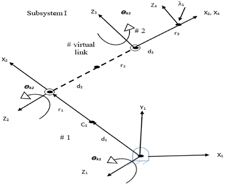
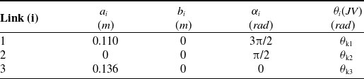
Thedelta robot is characterized by the Denavit–Hartenberg (DH) parameters, as shown in Table I. Voice coil actuator (VCA), i.e., the actuator having joint coordinates are given with variables θ1, θ2, θ3, θ4, θ5, θ6, θ7, θ8, θ9. Its geometric architecture is defined in Fig. 8 Table II.
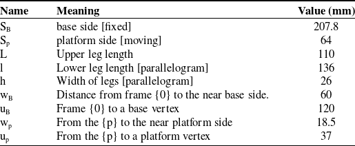
Parameters of the delta architecture.

Geometric architecture for subsystem I.

The DH parameters [Reference John28] of the kth leg of the delta platform.

Inverse kinematics of parallel robots is a process where actuated or active joint trajectories are to be computed for the respective poses of the platform motion. The inverse kinematics of parallel robots calculated both active and passive joint trajectories. The calculated results of inverse kinematics are needed for inverse dynamics to determine the driving torques/forces at the active joints.
3.3. Forward position kinematics solution [active joints]
The forward position kinematics is defined as the three actuated joint angles θ = {θ1, θ2, θ3} T are given then compute the resulting Cartesian position of the unfixed surface control point (P),
 $ \begin{array}{c}B\\ P\end{array}\textit{R}$
= {x y z} T. The forward position kinematics solution for parallel robots is tough.
Thecorrect solution set is selected for a straightforward analytical solution, as there is translation-only motion in the 3DOF delta robot. Given
 $ \Theta ={\left\{{\theta }_{1}{\theta }_{2}{\theta }_{3}\right\}}^{T}$
, then compute the three absolute vector knee points using
 $ \begin{array}{c}B\\ i\end{array}\textit{A}=\begin{array}{c}B\\ i\end{array}\textit{B}+\begin{array}{c}B\\ i\end{array}\textit{L},\textit{}\textit{i}=\textrm{1,2},3$
. The unfixed surface of the delta robot’s orientation is constant and horizontal with [
 $ \begin{array}{c}B\\ i\end{array}\textit{A}]=[{\textrm{I}}_{3}]$
; therefore, all the virtual sphere centres (three in number) are
 $ \begin{array}{c}B\\ iv\end{array}\textit{A}=\begin{array}{c}B\\ i\end{array}\textit{A}-\begin{array}{c}p\\ i\end{array}\textit{P},\textit{}\textit{i}=\textrm{1,2},3$
.
 \begin{align*} &{}_{1\textrm{v}}{}^{\textrm{B}}\textrm{A}=\left\{\begin{array}{c}0\\ \\[-7pt] {-\textrm{w}}_{\textrm{B}}-\textrm{L}\textrm{c}\textrm{o}\textrm{s}{{\theta }}_{1}+{\textrm{u}}_{\textrm{p}}\\ \\[-7pt] -\textrm{L}\textrm{s}\textrm{i}\textrm{n}{{\theta }}_{1}\end{array}\right\}\textrm{}\textrm{}\textrm{}\textrm{}\textrm{}\textrm{}\\[3pt]&{}_{2\textrm{v}}{}^{\textrm{B}}\textrm{A}=\left\{\begin{array}{c}\dfrac{\sqrt{3}}{2}\left({\textrm{w}}_{\textrm{B}}+\textrm{L}\textrm{c}\textrm{o}\textrm{s}{{\theta }}_{2}\right)-\dfrac{{\textrm{s}}_{\textrm{p}}}{2}\\ \\[-7pt] \dfrac{1}{2}\left({\textrm{w}}_{\textrm{B}}+\textrm{L}\textrm{c}\textrm{o}\textrm{s}{{\theta }}_{2}\right)-{\textrm{w}}_{\textrm{p}}\\ \\[-7pt] -\textrm{L}\textrm{s}\textrm{i}\textrm{n}{{\theta }}_{2}\end{array}\right\}\textrm{}\\[3pt]&{}_{3\textrm{v}}{}^{\textrm{B}}\textrm{A}=\left\{\begin{array}{c}-\dfrac{\sqrt{3}}{2}\left({\textrm{w}}_{\textrm{B}}+\textrm{L}\textrm{c}\textrm{o}\textrm{s}{{\theta }}_{3}\right)+\dfrac{{\textrm{s}}_{\textrm{p}}}{2}\\ \\[-7pt] \dfrac{1}{2}\left({\textrm{w}}_{\textrm{B}}+\textrm{L}\textrm{c}\textrm{o}\textrm{s}{{\theta }}_{3}\right)-{\textrm{w}}_{\textrm{p}}\\ \\[-7pt] -\textrm{L}\textrm{s}\textrm{i}\textrm{n}{{\theta }}_{3}\end{array}\right\}\end{align*}
Delta robot forward position kinematics is determined by its point of intersection of the three spheres. This sphere is represented by a centre point called c and the scalar radius defined by r.
In this section, an analytical solution is computed as the intersection point of the given three spheres. In this concern, it also needs to solve transcendental equations which is of coupled in nature. So, to solve the forward kinematics solution, an intersection-three-sphere algorithm exists. If this is the case when the entire three-sphere centres {
 $ \begin{array}{c}B\\ iv\end{array}\textit{A}$
} have the same height (Z), then the solution will be in the zone of the algorithmic singularity. To fix the problem rotating the coordinates, i.e., all {
 $ \begin{array}{c}B\\ iv\end{array}\textit{A}$
}, heights values are not the same.
As in this problem, two solutions were encountered when the three spheres intersect. When a sphere meeting is tangential, it results in one solution. The second case is an imaginary solution, and the data are inconsistent. The algorithm (spheres-intersection) compute solution sets, and the computer automatically chooses the solution below the base triangle. This approach to the forward position kinematics for the delta robot estimated results same as of solving the kinematics equations, depicted as
 $ \begin{array}{c}B\\ P\end{array}\textit{R}$
= {x y z} T given θ = {θ1, θ2, θ3} T.
3.4. Inverse position kinematics solution [active joints]
The inverse position kinematics problem is defined as the Cartesian position of the unfixed surface control point (P),
 $ \begin{array}{c}B\\ P\end{array}\textit{R}$
= {x y z}T are given then compute the three actuated revolute joint angles θ = {θ1, θ2, θ3} T. The inverse position kinematics solution delta robot is not trivial, therefore calculated analytically. The inverse position kinematics problem is not dependent on the three RUU legs of a delta robot; therefore, it can be solved individually for each leg. As shown in the figure above, geometrically, inverse position kinematics solution of each leg, the point of intersection between the known sphere (defined by radius l, and it is centre on the moving triangle vertex
 $ \begin{array}{c}P\\ i\end{array}\textit{P}$
) and known circle (defined by radius L, and it is centre on the fixed triangle R joint point
 $ \begin{array}{c}B\\ i\end{array}\textit{B}$
).
The inverse position kinematics solved both geometrically and trigonometrically. The inverse position kinematics are now solved analytically. The three independent scalar inverse position kinematics equations are shown below:
 \begin{align*} {\textrm{E}}_{\textrm{i}}\textrm{c}\textrm{o}\textrm{s}{{\theta }}_{\textrm{i}}+{\textrm{F}}_{\textrm{i}}\textrm{s}\textrm{i}\textrm{n}{{\theta }}_{\textrm{i}}+{\textrm{G}}_{\textrm{i}}=0,i=\textrm{1,2},3\end{align*}
where
 \begin{align} {\textrm{E}}_{1}=2L\left(y+a\right) {\textrm{F}}_{1}=2zL \end{align}
 \begin{align} {\textrm{}\textrm{G}}_{1}={x}^{2}+{y}^{2}+{z}^{2}+{a}^{2}+{L}^{2}+2ya-{l}^{2}\end{align}
 \begin{align} {\textrm{E}}_{2}=-L\left(\sqrt{3}\left(x+b\right)+y+c\right) {\textrm{F}}_{2}=2zL \end{align}
 \begin{align} {\textrm{}\textrm{G}}_{2}={x}^{2}+{y}^{2}+{z}^{2}+{b}^{2}+{c}^{2}+{L}^{2}+2xb+2yc-{l}^{2}\end{align}
 \begin{align} {\textrm{E}}_{3}=L\left(\sqrt{3}\left(x-b\right)-y-c\right),\textrm{}{\textrm{F}}_{3}=2zL\end{align}
 \begin{align} {\textrm{}\textrm{G}}_{3}={x}^{2}+{y}^{2}+{z}^{2}+{b}^{2}+{c}^{2}+{L}^{2}-2xb+2yc-{l}^{2}\end{align}
The equation
 $ {\textrm{E}}_{\textrm{i}}\textrm{c}\textrm{o}\textrm{s}{{\theta }}_{\textrm{i}}+{\textrm{F}}_{\textrm{i}}\textrm{s}\textrm{i}\textrm{n}{{\theta }}_{\textrm{i}}+{\textrm{G}}_{\textrm{i}}=0$
already used in robot, kinematics. A tangent half-angle solves it. If
 $ {\textrm{t}}_{\textrm{i}}=tan\frac{{{\theta }}_{\textrm{i}}}{2}$
, then
 $ \textrm{c}\textrm{o}\textrm{s}{{\theta }}_{\textrm{i}}=\frac{1-{t}_{i}^{2}}{1+{t}_{i}^{2}}$
and
 $ \textrm{s}\textrm{i}\textrm{n}{{\theta }}_{\textrm{i}}=\frac{2{t}_{i}}{1+{t}_{i}^{2}}$
. If tangent half-angle substituted into the EFG equation, then results below:
 \begin{align} &{\textrm{E}}_{\textrm{i}}\left(\frac{1-{t}_{i}^{2}}{1+{t}_{i}^{2}}\right)+ {\textrm{F}}_{\textrm{i}}\left(\frac{2{t}_{i}}{1+{t}_{i}^{2}}\right)+{\textrm{G}}_{\textrm{i}}=0\ {\textrm{E}}_{\textrm{i}}\left(1-{t}_{i}^{2}\right) + {\textrm{F}}_{\textrm{i}}\left(2{t}_{i}\right)+{\textrm{G}}_{\textrm{i}}(1+{t}_{i}^{2})=0 (1.37) \nonumber\\[3pt] &\quad {(\textrm{G}}_{\textrm{i}}-{\textrm{E}}_{\textrm{i}}){t}_{i}^{2}+(2{\textrm{F}}_{\textrm{i}}){t}_{i}+({\textrm{G}}_{\textrm{i}}+{\textrm{E}}_{\textrm{i}})=0\dots .\end{align}
Quadratic formula:
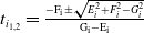 $ {t}_{{i}_{\textrm{1,2}}}=\frac{-{\textrm{F}}_{\textrm{i}}\pm \sqrt{{E}_{i}^{2}+{F}_{i}^{2}-{G}_{i}^{2}}}{{\textrm{G}}_{\textrm{i}}-{\textrm{E}}_{\textrm{i}}}$
. The
 $ {{\theta }}_{\textrm{i}}$
solved by inverting the original tangent, as shown below:
 \begin{align*} {{\theta }}_{\textrm{i}}=2{tan}^{-1}\left({\textrm{t}}_{\textrm{i}}\right)\end{align*}
Two solutions (positive and negative) are obtained from the quadratic formula. The first solution represents the knee left, and the second is the knee right of a delta robot. There are two possible solutions for each leg. Therefore, the eight possible solutions are there.
3.5. Delta robot velocity kinematics equations [active joints]
The velocity kinematics equations of the revolute-input delta robot are computed through the derivative of the position constraint equations.
 \begin{align} 2\textrm{L}\dot{\textrm{y}}\textrm{c}\textrm{o}\textrm{s}{{\theta }}_{1}-2\textrm{L}\left(\textrm{y}+\textrm{a}\right){\dot{\theta }}_{1}\textrm{s}\textrm{i}\textrm{n}{{\theta }}_{1}+2\textrm{L}\textrm{}\dot{\textrm{z}}\textrm{s}\textrm{i}\textrm{n}{{\theta }}_{1}+2\textrm{L}\textrm{z}{\dot{\theta }}_{1}\textrm{c}\textrm{o}\textrm{s}{{\theta }}_{1}+2\textrm{x}\dot{\textrm{x}\textrm{}}+2\left(\textrm{y}+\textrm{a}\right)\textrm{}\dot{\textrm{y}}+2\textrm{z}\dot{\textrm{z}}=0\end{align}
 \begin{align} &-\textrm{L}\left(\sqrt{3}\dot{\textrm{x}\textrm{}}+\dot{\textrm{y}}\right)\textrm{c}\textrm{o}\textrm{s}{{\theta }}_{2}+\textrm{L}\left(\sqrt{3(}\textrm{x}+\textrm{b}\right)+\textrm{y}+\textrm{c}){\dot{\theta }}_{2}\textrm{c}\textrm{o}\textrm{s}{{\theta }}_{2}+2\textrm{L}\dot{\textrm{z}}\textrm{s}\textrm{i}\textrm{n}{{\theta }}_{2}+2\textrm{L}\textrm{z}{\dot{\theta }}_{2}\textrm{c}\textrm{o}\textrm{s}{{\theta }}_{2}+2(\textrm{x}+\textrm{b})\dot{\textrm{x}\textrm{}}\nonumber\\ &\quad +2(\textrm{y}+\textrm{c})\dot{\textrm{y}\textrm{}}+2\textrm{z}\dot{\textrm{z}\textrm{}}=0\end{align}
 \begin{align} &\textrm{L}\left(\sqrt{3}\dot{\textrm{x}\textrm{}}-\dot{\textrm{y}\textrm{}}\right)\textrm{c}\textrm{o}\textrm{s}{{\theta }}_{3}-\textrm{L}\left(\sqrt{3}\left(\textrm{x}-\textrm{b}\right)-\textrm{y}-\textrm{c}\right){\dot{\theta }}_{3}\textrm{s}\textrm{i}\textrm{n}{{\theta }}_{3}+2\textrm{L}\dot{\textrm{z}}{\dot{\theta }}_{3}\textrm{s}\textrm{i}\textrm{n}{{\theta }}_{3}+2\textrm{L}\textrm{z}\textrm{c}\textrm{o}\textrm{s}{{\theta }}_{3}-2\left(\textrm{x}-\textrm{b}\right)\dot{\textrm{x}\textrm{}}\textrm{}\nonumber\\ &\quad +2\left(\textrm{y}+\textrm{c}\right)\dot{\textrm{y}\textrm{}}\textrm{}+2\textrm{z}\dot{\textrm{z}\textrm{}}\textrm{}=0\end{align}
Equation 15, 16, and 17 can be re-written as
 \begin{align} \textrm{x}\dot{\textrm{x}\textrm{}}\textrm{}+\left(\textrm{y}+\textrm{a}\right)\dot{\textrm{y}\textrm{}}+\textrm{L}\dot{\textrm{y}\textrm{}}\textrm{c}\textrm{o}\textrm{s}{{\theta }}_{1}+\textrm{z}\dot{\textrm{z}\textrm{}}\textrm{}+\textrm{L}\dot{\textrm{z}\textrm{}}\textrm{s}\textrm{i}\textrm{n}{{\theta }}_{1}=\textrm{L}\left(\textrm{y}+\textrm{a}\right){\dot{\theta }}_{1}\textrm{s}\textrm{i}\textrm{n}{{\theta }}_{1}-\textrm{L}\textrm{z}{\dot{\theta }}_{1}\textrm{c}\textrm{o}\textrm{s}{{\theta }}_{1}\end{align}
 \begin{align} &2\left(\textrm{x}+\textrm{b}\right)\dot{\textrm{x}\textrm{}}+2\left(\textrm{y}+\textrm{c}\right)\dot{\textrm{y}\textrm{}}-\textrm{L}\left(\sqrt{3}\dot{\textrm{x}\textrm{}}+\dot{\textrm{y}\textrm{}}\right)\textrm{c}\textrm{o}\textrm{s}{{\theta }}_{2}+2\textrm{z}\dot{\textrm{z}\textrm{}}+2\textrm{L}\dot{\textrm{z}}\textrm{s}\textrm{i}\textrm{n}{{\theta }}_{2}\nonumber\\[3pt] &\quad =-\textrm{L}\left(\sqrt{3}\left(\textrm{x}+\textrm{b}\right)+\textrm{y}+\textrm{c}\right){\dot{\theta }}_{2}\textrm{s}\textrm{i}\textrm{n}{{\theta }}_{2}-2\textrm{L}\textrm{z}{\dot{\theta }}_{2}\textrm{c}\textrm{o}\textrm{s}{{\theta }}_{2}\end{align}
 \begin{align} & 2\left(\textrm{x}-\textrm{b}\right)\dot{\textrm{x}\textrm{}}+2\left(\textrm{y}+\textrm{c}\right)\dot{\textrm{y}}+\textrm{L}\left(\sqrt{3}\dot{\textrm{x}\textrm{}}-\dot{\textrm{y}}\right)\textrm{c}\textrm{o}\textrm{s}{{\theta }}_{3}+2\textrm{z}\dot{\textrm{z}}+2\textrm{L}\dot{\textrm{z}}\textrm{s}\textrm{i}\textrm{n}{{\theta }}_{3}\nonumber\\[3pt] &\quad =-\textrm{L}\left(\sqrt{3}\left(\textrm{x}-\textrm{b}\right)-\textrm{y}-\textrm{c}\right){\dot{\theta }}_{3}\textrm{s}\textrm{i}\textrm{n}{{\theta }}_{3}-2\textrm{L}\textrm{z}{\dot{\theta }}_{3}\textrm{c}\textrm{o}\textrm{s}{{\theta }}_{3}\end{align}
In matrix-vector form:
 $ \left[\textrm{A}\right]\{\dot{\textrm{X}\}=\left[\textrm{B}\right]\{\dot{{\theta }\}}}$
 \begin{align} \left[\begin{array}{c@{\quad}c@{\quad}c}\textrm{x}& \textrm{y}+\textrm{a}+\textrm{L}\textrm{c}\textrm{o}\textrm{s}{{\theta }}_{1}& \textrm{z}+\textrm{L}\textrm{s}\textrm{i}\textrm{n}{{\theta }}_{1}\\ \\[-7pt]2\left(\textrm{x}+\textrm{b}\right)-\sqrt{3}\textrm{L}\textrm{c}\textrm{o}\textrm{s}{{\theta }}_{2} &2\left(\textrm{y}+\textrm{c}\right)-\textrm{L}\textrm{c}\textrm{o}\textrm{s}{{\theta }}_{2}& 2(\textrm{z}+\textrm{L}\textrm{s}\textrm{i}\textrm{n}{{\theta }}_{2})\\ \\[-7pt] 2\left(\textrm{x}-\textrm{b}\right)+\sqrt{3}\textrm{L}\textrm{c}\textrm{o}\textrm{s}{{\theta }}_{3} &2\left(\textrm{y}+\textrm{c}\right)-\textrm{L}\textrm{c}\textrm{o}\textrm{s}{{\theta }}_{3}& 2(\textrm{z}+\textrm{L}\textrm{s}\textrm{i}\textrm{n}{{\theta }}_{3})\end{array}\right]\left\{\begin{array}{c}\dot{\textrm{x}}\\ \\[-7pt] \dot{\textrm{y}}\\ \\[-7pt] \dot{\textrm{z}}\end{array}\right\}=\left[\begin{array}{c@{\quad}c@{\quad}c}{\textrm{b}}_{11}& 0& 0\\ \\[-7pt] 0& {\textrm{b}}_{22}& 0\\ \\[-7pt] 0& 0& {\textrm{b}}_{33}\end{array}\right]\left\{\begin{array}{c}\dot{{{\theta }}_{1}}\\ \\[-7pt] \dot{{{\theta }}_{2}}\\ \\[-7pt] \dot{{{\theta }}_{3}}\end{array}\right\}\end{align}
where
 $ {\textrm{b}}_{11}=\textrm{L}[(\textrm{y}+\textrm{a})\textrm{s}\textrm{i}\textrm{n}{{\theta }}_{1}-\textrm{z}\textrm{c}\textrm{o}\textrm{s}{{\theta }}_{1}];\,\, {\textrm{b}}_{22}=-\textrm{L}[(\sqrt{3}(\textrm{x}+\textrm{b})+\textrm{y}+\textrm{c})\textrm{s}\textrm{i}\textrm{n}{{\theta }}_{2}+2\textrm{z}\textrm{c}\textrm{o}\textrm{s}{{\theta }}_{2}]$
 $ {\textrm{b}}_{33}=\textrm{L}[(\sqrt{3}(\textrm{x}-\textrm{b})-\textrm{y}-\textrm{c})\textrm{s}\textrm{i}\textrm{n}{{\theta }}_{3}-2\textrm{z}\textrm{c}\textrm{o}\textrm{s}{{\theta }}_{3}]$
3.6. Inverse position kinematics solution [active and passive joints]
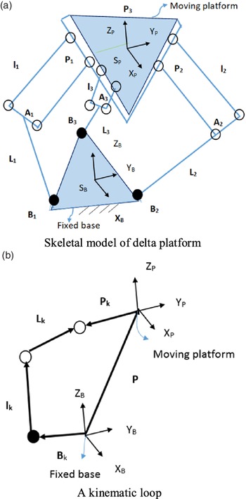
In kinematic and dynamic analyses, the moving platform is assumed to be cut at three spherical joints and detached from the three identical legs. As shown in Fig. 6(a), the three-DOF delta platform has a fixed base connected to three identical legs through universal joints at three different points, namely, at Ai’s. These legs are connected to the platform (moving) through three spherical joints at Bi’s. Each leg consists of two links connected with a universal joint denoted as Ui’s. Therefore, each leg has three-DOF. Referring to Fig. 6(b), the loop-closure equation for the kth loop is given as
 \begin{align} \overrightarrow{{B}_{i}}+\overrightarrow{{L}_{i}}+\textrm{}\overrightarrow{{l}_{i}}=\overrightarrow{P}+\textrm{}{p}_{i} \end{align}
 \begin{align} \overrightarrow{{L}_{i}}+\textrm{}\overrightarrow{{l}_{i}}=\left[\begin{array}{c}x\\ y\\ z\end{array}\right]+\left[\begin{array}{c}0\\ -{\textrm{u}}_{\textrm{p}}\\ 0\end{array}\right]-\textrm{}\left[\begin{array}{c}0\\ -{\textrm{w}}_{\textrm{B}}\\ 0\end{array}\right]\end{align}
 $ \overrightarrow{{\textrm{L}}_{\textrm{i}}}+\overrightarrow{{\textrm{l}}_{\textrm{i}}}$
can be found using the D-H parameter approach.
 $ \overrightarrow{{\textrm{L}}_{\textrm{i}}}$
is the vector from the base vertex and corresponding platform vertex, i.e., from Ai to Bi. The magnitude of this vector also represents leg length for the respective platform motion. Vector p is the measure of the displacement of the platform to the base. Here
 $\text{'}$
p’ represents the position vector of point
 $\text{'}$
P’ on the platform from the centre of the base, i.e., points O,
 $ \overrightarrow{{\textrm{L}}_{\textrm{i}}}\textrm{}and\textrm{}\overrightarrow{{\textrm{l}}_{\textrm{i}}}$
are the vectors locating the vertices of the base and platform in their respective frames, i.e., XYZ and Xp, Yp, Zp as depicted in Fig.6(a). Since the platform has three-DOF, its motion can be represented by three independent translations and about axes Xp, Yp, and Zp. If the values of xp, yp, zp, the vector
 $ {\textrm{a}}_{\textrm{k}}\textrm{}$
can be calculated from Eq. 2. The coordinate values of the base and platform vertices, i.e., AI, AIII, and BI…, BIX are taken from the CAD model to calculate the active and passive joint trajectories. The homogeneous transformation matrix between frame 3 and frame 1 can be given as the homogeneous transformation matrix (HTM).
 \begin{align} {T}_{k}\equiv \left[\begin{array}{c@{\quad}c@{\quad}c@{\quad}c}{C\theta }_{ki}& {-S\theta }_{ki}{C\alpha }_{ki} & {-S\theta }_{ki}{S\alpha }_{ki}& {{a}_{i}C\theta }_{ki}\\ \\[-7pt] {S\theta }_{ki}& {C\theta }_{ki}{C\alpha }_{ki} & {-C\theta }_{ki}{S\alpha }_{ki}& {{a}_{ki}S\theta }_{ki}\\ \\[-7pt] 0& {\textrm{}\textrm{}\textrm{}\textrm{}\textrm{}\textrm{}\textrm{}S\alpha }_{ki}& {C\alpha }_{ki}&{b}_{ki}\\ \\[-7pt] 0& 0 & 0&1\end{array}\right]\end{align}
Consider
 $,{a}_{2}=0$
;
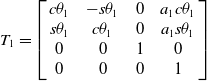 $ {T}_{1}=\left[\begin{array}{c@{\quad}c@{\quad}c@{\quad}c}c{\theta }_{1} &-s{\theta }_{1} &0& {a}_{1}c{\theta }_{1}\\s{\theta }_{1} &c{\theta }_{1} &0& {a}_{1}s{\theta }_{1}\\0& 0&1&0\\ 0 &0& 0&1 \end{array}\right]$
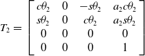 $ \textrm{}\textrm{}\textrm{}\textrm{}\textrm{}\textrm{}\textrm{}\textrm{}\textrm{}\textrm{}\textrm{}\textrm{}\textrm{}\textrm{}\textrm{}\textrm{}\textrm{}\textrm{}{T}_{2}=\textrm{}\textrm{}\textrm{}\textrm{}\textrm{}\textrm{}\left[\begin{array}{c@{\quad}c@{\quad}c@{\quad}c}c{\theta }_{2} &0 & -s{\theta }_{2}& {a}_{2}c{\theta }_{2}\\s{\theta }_{2}& 0 & c{\theta }_{2}& {a}_{2}s{\theta }_{2}\\ 0&0&0&0\\0&0&0&1\\\end{array}\right]$
 \begin{align*} {T}_{1}{T}_{2}{T}_{3}=\left[\begin{array}{c@{\quad}c@{\quad}c@{\quad}c}c{\theta }_{12}c{\theta }_{3}& -c{\theta }_{12}s{\theta }_{3} & \textrm{}\textrm{}-s{\theta }_{12}& {\textrm{}\textrm{}\textrm{}a}_{1}c{\theta }_{1}+{a}_{2}c{\theta }_{12}\\ \\[-7pt]s{\theta }_{12}c{\theta }_{3} &-s{\theta }_{12}s{\theta }_{3} & \textrm{}\textrm{}c{\theta }_{12}& {\textrm{}\textrm{}\textrm{}a}_{1}s{\theta }_{1}+\textrm{}{a}_{2}s{\theta }_{12}\\ \\[-7pt]-s{\theta }_{3}& -c{\theta }_{3}& 0&{-a}_{3}s{\theta }_{3}\\ \\[-7pt]0& 0 &0&1\\\end{array}\right]\end{align*}
Using equation 24 and putting in the triangular frame, represented as
 \begin{align} \overrightarrow{{L}_{i}}+\textrm{}\overrightarrow{{l}_{i}}=\left[\begin{array}{c}{-a}_{3}s{\theta }_{3}\\ \\[-7pt] {\textrm{}\textrm{}\textrm{}a}_{1}c{\theta }_{1}+{a}_{2}c{\theta }_{12}\\ \\[-7pt] {\textrm{}\textrm{}\textrm{}a}_{1}s{\theta }_{1}+\textrm{}{a}_{2}s{\theta }_{12}\end{array}\right],\end{align}
 \begin{align} \overrightarrow{{L}_{i}}+\textrm{}\overrightarrow{{l}_{i}}=\textrm{}\textrm{}\left[\begin{array}{c}x\\ \\[-7pt] y1\textrm{}\\ \\[-7pt] z\end{array}\right] \end{align}
where
 $y1=y-{\textrm{u}}_{\textrm{p}}+{\textrm{w}}_{\textrm{B}}$
 \begin{align*} {-a}_{3}s{\theta }_{3}=x\\[3pt] {\theta }_{3}=\textrm{}-{\textit{sin}}^{-1}(x/{a}_{3}) \end{align*}
Using equations 25 and 26, square and adding resulted in the computation of the
 $ {\theta }_{2}$
 \begin{align*} {\theta }_{2}=\textrm{}-{\textit{sin}}^{-1}\left(k\right)\end{align*}
where k = (x2 + y2 + z2 – a1
2 – a3
2/2a1a3
 $ c{\theta }_{3}$
)
 \begin{align} y1=\textrm{} {\textrm{}\textrm{}\textrm{}a}_{1}c{\theta }_{1}+{a}_{2}c{\theta }_{12}\end{align}
 \begin{align} z\textrm{}\, {\textrm{}\textrm{}\textrm{}a}_{1}s{\theta }_{1}+\textrm{}{a}_{2}s{\theta }_{12} .\end{align}
 \begin{align} y1\textrm{}\textrm{*}\textrm{}\left({\textrm{}\textrm{}\textrm{}a}_{3}s{\theta }_{2}c{\theta }_{3}\right)\textrm{}=\textrm{} {\textrm{}\textrm{}\textrm{}a}_{1}c{\theta }_{1}+{a}_{2}c{\theta }_{12} \,{}^{*}\,{\textrm{}\textrm{}\textrm{}a}_{3}s{\theta }_{2}c{\theta }_{3}) \end{align}
 \begin{align} z\textrm{*}\left({a}_{1}+{a}_{3}c{\theta }_{2}c{\theta }_{3}\right) {a}_{1}s{\theta }_{1}+\textrm{}{a}_{2}s{\theta }_{12} \,{}^{*}\, ({a}_{1}+{a}_{3}c{\theta }_{2}c{\theta }_{3})\end{align}
Multiplying
 $ {a}_{3}s{\theta }_{2}c{\theta }_{3}$
in equations 27 and
 $ {a}_{1}+{a}_{3}c{\theta }_{2}c{\theta }_{3}$
in equation 28 and termed the equations 29 and 30, respectively. Using equations 29 and 30 and subtracting equation 27 from equation 28 resulted in the computation of the
 $ {\theta }_{1}$
.
 \begin{align*} {\theta }_{1}=\textrm{}{\textit{tan}}^{-1}\left(q\right)\end{align*}
 \begin{align} \textrm{where} q = (z ( {a}_{1}+{a}_{3}c{\theta }_{2}c{\theta }_{3})-y1 ( {a}_{3}s{\theta }_{2}c{\theta }_{3} )/z ( {a}_{1}+{a}_{3}c{\theta }_{2}c{\theta }_{3}) + y1 ( {a}_{3}s{\theta }_{2}c{\theta }_{3}))\end{align}
Kinematic loop closure equation inherited from the equations 25 and 26, represented as
 \begin{align} \left[\begin{array}{c}{-a}_{3}s{\theta }_{3}\\ \\[-7pt] {\textrm{}\textrm{}\textrm{}a}_{1}c{\theta }_{1}+{a}_{2}c{\theta }_{12}\\ \\[-7pt] {\textrm{}\textrm{}\textrm{}a}_{1}s{\theta }_{1}+\textrm{}{a}_{2}s{\theta }_{12}\end{array}\right]=\textrm{}\textrm{}\left[\textrm{}\begin{array}{c}x\\ \\[-7pt] y1\textrm{}\\ \\[-7pt] z\end{array}\right] \end{align}
Differentiate equation 32 with respect to the time
 \begin{align*} &-{a}_{3}c{\theta }_{3}\dot{{\theta }_{3}}=\textrm{}\dot{\textrm{x}}\textrm{}\\ &{a}_{3}\left(-c{\theta }_{3}s{\theta }_{12}\dot{{\theta }_{12}}-\textrm{}s{\theta }_{3}c{\theta }_{12}\dot{{\theta }_{3}}\textrm{}\right)-\textrm{}{a}_{1}s{\theta }_{1}\dot{{\theta }_{1}=} \textrm{}\dot{\textrm{y}1}\\ & {a}_{3}\left(c{\theta }_{3}c{\theta }_{12}\dot{{\theta }_{12}}-\textrm{}s{\theta }_{3}s{\theta }_{12}\dot{{\theta }_{3}}\textrm{}\right)+\textrm{}{a}_{1}c{\theta }_{1}\dot{{\theta }_{1}=} \textrm{}\dot{\textrm{z}}\end{align*}
 $ [J \dot{{\theta }}=\dot{\overrightarrow{X}}$
] represented as
 \begin{align} \left[\begin{array}{c@{\quad}c@{\quad}c}0&-{a}_{3}c{\theta }_{3}\dot{{\theta }_{3}}&0\\ \\[-7pt] {-a}_{1}s{\theta }_{1}-{a}_{3}c{\theta }_{3}s{\theta }_{12}&-{a}_{3}c{\theta }_{3}s{\theta }_{12}&-{a}_{3}s{\theta }_{3}c{\theta }_{12}\\ \\[-7pt] \textrm{}{a}_{1}c{\theta }_{1}+{a}_{3}c{\theta }_{3}c{\theta }_{12}&{a}_{3}c{\theta }_{3}c{\theta }_{12}\textrm{}\textrm{}\textrm{}\textrm{}\textrm{}-{a}_{3}s{\theta }_{3}s{\theta }_{12}\end{array}\right]\left[\begin{array}{c}\dot{{\theta }_{1}}\\ \\[-7pt] \dot{{\theta }_{2}}\\ \\[-7pt] \dot{{\theta }_{3}}\end{array}\right] &= \left[\begin{array}{c}\dot{x}\\ \\[-7pt] \dot{y}\\ \\[-7pt] \dot{z}\end{array}\right]\textrm{}\textrm{}\dots. \nonumber\\[3pt] \left[J\right]\left[\begin{array}{c}\dot{{\theta }_{1}}\\ \\[-7pt] \dot{{\theta }_{2}}\\ \\[-7pt] \dot{{\theta }_{3}}\end{array}\right]&=\left[\begin{array}{c}\dot{x}\\ \\[-7pt] \dot{y}\\ \\[-7pt] \dot{z}\end{array}\right] \end{align}
Again, foracceleration level, differentiate equation 1.57 to the
 $ \dot{{\theta }}$
and represented as
 \begin{align} J\textrm{}\ddot{\theta }+\dot{J}\dot{\theta }=\ddot{\overrightarrow{X\textrm{}}}\end{align}
where
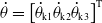 $ \dot{{\theta }}={\left[{\dot{{\theta }}}_{\textrm{k}1}\textrm{}{\dot{{\theta }}}_{\textrm{k}2\textrm{}}{\dot{{\theta }}}_{\textrm{k}3}\right]}^{\textrm{T}}$
and Jk is the 3×3 Jacobian matrix related to the serial chain of the kth leg. The Jacobian matrix Jk can be obtained by differentiating the first three elements of the last column of the homogeneous transformation matrix Tk.
 \begin{align} J_{k} \equiv \left[\begin{array}{c@{\quad}c@{\quad}c}0&-{a}_{3}c{\theta }_{3}\dot{{\theta }_{3}}&0\\ \\[-7pt] {-a}_{1}s{\theta }_{1}-{a}_{3}c{\theta }_{3}s{\theta }_{12}&-{a}_{3}c{\theta }_{3}s{\theta }_{12}&-{a}_{3}s{\theta }_{3}c{\theta }_{12}\\ \\[-7pt] {a}_{1}c{\theta }_{1}+{a}_{3}c{\theta }_{3}c{\theta }_{12}&{a}_{3}c{\theta }_{3}c{\theta }_{12}&-{a}_{3}s{\theta }_{3}s{\theta }_{12}\end{array}\right]\end{align}
Similarly differentiating Eq. 34, the joint acceleration can be derived as
 \begin{align} \ddot{\theta }={J}_{k}^{-1}(\ddot{{l}_{k}}-{\dot{J}}_{k}{\dot{\theta }}_{k})\end{align}
where
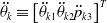 $ {\ddot{\theta }}_{k}\equiv {\left[{\ddot{\theta }}_{k1}{\ddot{\theta }}_{k2}{\ddot{p}}_{k3}\right]}^{T}$
. The derivative of the Jacobian matrix,
 $ {\dot{J}}_{k}\equiv \left[{\dot{J}}_{1k}{\dot{J}}_{2k}{\dot{J}}_{3k}\right]$
in Eq. 2 is as follows:
 \begin{align} {j}_{1k}\equiv \left[\begin{array}{c}0\textrm{}\textrm{}\\ \\[-7pt] {-a}_{1}c{\theta }_{1}\dot{{\theta }_{1}}-{a}_{3}(c{\theta }_{3}c{\theta }_{12}\dot{{\theta }_{12}}-\textrm{}s{\theta }_{3}s{\theta }_{12}\dot{{\theta }_{3}})\textrm{}\\ \\[-7pt] {-a}_{1}s{\theta }_{1}\dot{{\theta }_{1}}-{a}_{3}(c{\theta }_{3}s{\theta }_{12}\dot{{\theta }_{12}}-\textrm{}s{\theta }_{3}c{\theta }_{12}\dot{{\theta }_{3}})\textrm{}\textrm{}\end{array}\right]\end{align}
 \begin{align} {j}_{2k}\equiv \left[\begin{array}{c}0\textrm{}\textrm{}\\ \\[-7pt] {\textrm{}\textrm{}\textrm{}\textrm{}\textrm{}-a}_{3}(c{\theta }_{3}c{\theta }_{12}\dot{{\theta }_{12}}-s{\theta }_{3}s{\theta }_{12}\dot{{\theta }_{3}})\textrm{}\textrm{}\textrm{}\textrm{}\textrm{}\textrm{}\\ \\[-7pt] {-a}_{3}{(c\theta }_{3}s{\theta }_{12}\dot{{\theta }_{12}}+c{\theta }_{3}c{\theta }_{12}\dot{{\theta }_{3}})\textrm{}\textrm{}\end{array}\right]\end{align}
 \begin{align} {j}_{3k}\equiv \left[\begin{array}{c}{\textrm{}\textrm{}\textrm{}\textrm{}\textrm{}a}_{3}s{\theta }_{3}\dot{{\theta }_{3}}\textrm{}\textrm{}\\ \\[-7pt] {\textrm{}\textrm{}\textrm{}\textrm{}\textrm{}-a}_{3}(-s{\theta }_{3}s{\theta }_{12}\dot{{\theta }_{12}}+c{\theta }_{3}c{\theta }_{12}\dot{{\theta }_{3}})\textrm{}\textrm{}\textrm{}\textrm{}\\ \\[-7pt] {-a}_{3}{(s\theta }_{3}c{\theta }_{12}\dot{{\theta }_{12}}+c{\theta }_{3}s{\theta }_{12}\dot{{\theta }_{3}})\textrm{}\textrm{}\end{array}\right]\end{align}
4. Dynamics Analysis
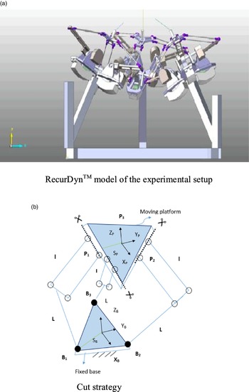
The mechanism model of the parallel delta robot is shown in Fig. 9(a), which has a fixed base and a moving platform. Each leg has two links, the first link is connected to the base and the second link by revolute joint and spherical joint, respectively, while the second link is connected to the platform by spherical joint. The base joints (revolute) are active. To simplify the dynamics of the delta robot, it is divided into four subsystems, as shown in Fig.10(b), and to compensate, Lagrange multipliers are used. The subsystems one, two, and three can be considered two-link manipulators with three-degree-of-freedom (since the rotation of the second link about its axis is not considered), in the effect of Lagrange multipliers. Since the legs of the delta robot are identical, we only need to derive the dynamic equation of one leg and the moving platform. Combining the above-said dynamics resulted in the dynamics of the delta robots for performing the catching.
(a) Skeletal model of delta platform. (b) A kinematic loop.

(a) RecurDynTM model of the experimental setup. (b) Cut strategy.

4.1. Dynamics of the legs
The dynamic analysis of the delta robot is performed using the DeNOC formulation [give reference]. Subsystem one, i.e., leg 1, has two links but three-DOF; therefore, to derive the dynamic equations, a virtual link was introduced to make the number of links equal to the degree of freedom of the leg. The unconstraint Newton–Euler equations for the i th link of the k th leg can be expressed as
 \begin{align} {I}_{ik}{\omega }_{ik}+{\omega }_{ik}\textrm{}\times \textrm{}{I}_{ik}{\omega }_{ik}={n}_{ik}\nonumber\\[3pt] {m}_{ik}{\ddot{c}}_{ik}={f}_{ik} \end{align}
where
 $ {I}_{ik}$
and
 $ {m}_{ik}$
are the inertia tensor and mass of the link, respectively,
 $ {\omega }_{ik}$
and
 $ {\ddot{c}}_{ik}$
are the angular velocity and linear velocity of centre-of-mass (COM), respectively, while
 $ {\omega }_{ik}$
and
 $ {\ddot{c}}_{ik}$
are their corresponding time derivative,
 $ {n}_{ik}$
and
 $ {f}_{ik}$
are the moment and force about/at the COM of the link, respectively. The above expression can be written in matrix-vector as given below
 \begin{align} {M}_{ik}{\dot{t}}_{ik}+{W}_{ik}{M}_{ik}{t}_{ik}={\omega }_{ik}\end{align}
where
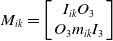 $ {M}_{ik}=\left[\begin{array}{cc}{I}_{ik} {O}_{3}\\ {O}_{3} {m}_{ik}{I}_{3}\end{array}\right]$
is the mass matrix,
 $ {t}_{ik}=\left[\begin{array}{c}{\omega }_{ik}\\ {\dot{c}}_{ik}\end{array}\right]$
is the twist vector,
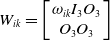 $ {W}_{ik}=\left[\begin{array}{cc}{\omega }_{ik}{I}_{3} {O}_{3}\\ {O}_{3} {O}_{3}\end{array}\right]$
is the angular velocity matrix,
 $ {\omega }_{ik}=\left[\begin{array}{c}{n}_{ik}\\ {f}_{ik}\end{array}\right]$
is the wrench vector, and
 $ {1}_{3}$
and
 $ {\textit{O}}_{3}$
are 3x3 identity and null matrix, respectively. The unconstraint equations for the k
th leg can be written as
 \begin{align} {M}_{ik}{\dot{t}}_{ik}+{W}_{ik}{M}_{ik}{t}_{ik}={\omega }_{ik}\end{align}
where
 $ {M}_{k}=diag\left[\begin{array}{cc}{M}_{1k} \begin{array}{cc}{M}_{2k} {M}_{3k}\end{array}\end{array}\right]$
 \begin{align*} \textrm{}\textrm{}\textrm{}\textrm{}\textrm{}\textrm{}\textrm{}\textrm{}\textrm{}\textrm{}\textrm{}\textrm{}\textrm{}{W}_{k}=diag\left[\begin{array}{cc}{W}_{1k} \begin{array}{cc}{W}_{2k} {W}_{3k}\end{array}\end{array}\right]\\[3pt]\textrm{}\textrm{}\textrm{}\textrm{}\textrm{}\textrm{}\textrm{}\textrm{}\textrm{}\textrm{}\textrm{}\textrm{}\textrm{}\textrm{}{t}_{k}={\left[\begin{array}{cc}{t}_{1k} \begin{array}{cc}{t}_{2k} {t}_{3k}\end{array}\end{array}\right]}^{T}\\[3pt]{\textrm{}w}_{k}={\left[\begin{array}{cc}{w}_{1k} \begin{array}{cc}{w}_{2k} {w}_{3k}\end{array}\end{array}\right]}^{T}\end{align*}
4.1.1. Derivation of DeNOC matrices through kinematic constraints
The angular velocity and linear velocity of COM of the links in k th can be written in recursive as given below
 \begin{align} {\omega }_{1k}&={\dot{\theta }}_{1k}{e}_{1k} \nonumber\\[3pt] {\dot{c}}_{1k}&={\omega }_{1k}\times {d}_{1k}={\dot{\theta }}_{1k}{e}_{1k}\times {d}_{1k}\end{align}
 \begin{align} {\omega }_{2k}&={\omega }_{1k}+{\dot{\theta }}_{2k}{e}_{2k} \nonumber\\[3pt] {\dot{c}}_{2k}&={\textrm{}{\dot{c}}_{1k}+\textrm{}\omega }_{1k}\times {({r}_{1k}+d}_{2k})+{\dot{\theta }}_{2k}{e}_{2k}\times {d}_{2k}\end{align}
 \begin{align} {\omega }_{3k}&={\omega }_{3k}+{\dot{\theta }}_{3k}{e}_{3k} \nonumber \\[3pt] {\dot{c}}_{3k}&={\textrm{}{\dot{c}}_{2k}+\textrm{}\omega }_{2k}\times {({r}_{2k}+d}_{3k})+{\dot{\theta }}_{3k}{e}_{3k}\times {d}_{3k} \\[-5pt]\nonumber\end{align}
The corresponding twist vector for each link of the k th leg can be expressed as
 \begin{align} {t}_{1k}={p}_{1k}{\dot{\theta }}_{1k};\ \textrm{}{t}_{2k}={B}_{\textrm{2,1}k}{t}_{1k}+{p}_{2k}{\dot{\theta }}_{2k};\ {t}_{3k}={B}_{\textrm{3,2}k}{t}_{2k}+{p}_{2k}{\dot{\theta }}_{3k}\end{align}
where
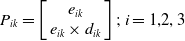 $ {P}_{ik}=\left[\begin{array}{c}{e}_{ik}\\ {e}_{ik}\times {d}_{ik}\end{array}\right];\ i=\textrm{1,2},3$
 \begin{align*} {B}_{i,i-1k}=\left[\begin{array}{c@{\quad}c}{1}_{3}& {O}_{3}\\ {c}_{i,i-1k}\times {1}_{3}& {1}_{3}\end{array}\right] \nonumber\\[3pt] {\textrm{}c}_{i,i-1k}=-\left({r}_{i-1k}+{d}_{ik}\right);i=\textrm{2,3}. \end{align*}
The above twist vector can be written as
 $ {t}_{k}={N}_{k}{\dot{\theta }}_{k}$
with
 $ {N}_{k}={N}_{lk}{N}_{dk}$
where
 \begin{align*} {N}_{lk}\equiv \left[\begin{array}{c@{\quad}c@{\quad}c}{1}_{6} &{O}_{6}& {O}_{6}\\ \\[-7pt] {B}_{\textrm{2,1}k}& {1}_{6}& {O}_{6}\\ \\[-7pt] {B}_{\textrm{3,1}k} &{B}_{\textrm{3,2}k}& {1}_{6}\end{array}\right];\ {N}_{dk}\equiv \left[\begin{array}{c@{\quad}c@{\quad}c}{P}_{1k}& \phi & \phi \\ \\[-7pt] \phi & {P}_{2k}& \phi \\ \\[-7pt] \phi & \phi & {P}_{3k}\end{array}\right];\ {\dot{\theta }}_{k}\equiv \left[\begin{array}{c}{\dot{\theta }}_{1k}\\ \\[-7pt] {\dot{\theta }}_{2k}\\ \\[-7pt] {\dot{\theta }}_{3k}\end{array}\right]\end{align*}
 $ {1}_{6}$
and
 $ {O}_{6}$
are the
 $ 6\times 6$
identity and null matrix, respectively, while
 $\phi $
is the
 $ 6\times 1$
zero vector.The
 $ 6\times 6$
matrix
 $ {B}_{\textrm{3,1}k}$
is the matrix multiplication of
 $ {B}_{\textrm{3,2}k}{B}_{\textrm{2,1}k}$
. The above
 $ {N}_{k}$
matrix is known as the Natural Orthogonal Complement (NOC) matrix, and its decoupled form
 $ {N}_{lk}{N}_{dk}$
is known as Decoupled NOC, which would be used to project the unconstraint equations of motion on the kinematic constraint space as given below:
 \begin{align} {N}_{dk}^{T}{N}_{lk}^{T}\left\{{M}_{k}{\dot{t}}_{k}+{W}_{k}{M}_{k}{t}_{k}\right\}={N}_{dk}^{T}{N}_{lk}^{T}{w}_{k}\end{align}
 \begin{align} {I}_{k}\left({\theta }_{k}\right){\ddot{\theta }}_{k}+{C}_{k}\left({\theta }_{k},{\dot{\theta }}_{k}\right){\dot{\theta }}_{k}=-{\gamma }_{k}+{\tau }_{k}\\ \nonumber \end{align}
where
 $ {I}_{k}\left({\theta }_{k}\right)\equiv {N}_{k}^{T}{M}_{k}{N}_{k}$
is the generalized inertia matrix (GIM);
 $ {C}_{k}\left({\theta }_{k},{\dot{\theta }}_{k}\right)\equiv {N}_{k}^{T}\left[{M}_{k}{\dot{N}}_{k}+{W}_{k}{M}_{k}{N}_{k}\right]$
is the matrix of Coriolis forces; and
 $ -{\gamma }_{k}+{\tau }_{k}\equiv {N}_{k}^{T}{w}_{k}$
in which
 $ {\gamma }_{k}$
the generalized is the force due to gravity and
 $ {\tau }_{k}$
represents the actuator torques. The above equations of motion considering the Lagrange multipliers
 ${\bf{\lambda }}$
can be expressed as
 \begin{align} {I}_{k}\left({\theta }_{k}\right){\ddot{\theta }}_{k}+{C}_{k}\left({\theta }_{k},{\dot{\theta }}_{k}\right){\ddot{\theta }}_{k}+{\gamma }_{k}={J}_{k}^{T}{}_{k}+{\tau }_{k}\end{align}
where
 $ {J}_{k}$
is the Jacobian matrix and
 $k = 1,2,3.$
4.2. Dynamics of the platform
The platform is shown in Fig. 11. The local frame attached to the centroid
 $ {0}_{p}$
of platform is
 $ {X}_{p}-{Y}_{p}-{Z}_{p}$
. The platform can only translate in 3D space, and therefore, the rotation matrix between the base frame and the platform frame is the identity matrix. The platform is connected to the legs at points
 $ {p}_{1},{p}_{2}$
, and
 $ {p}_{3}$
. The position vector of the moving platform with respect to the base frame is given below
 \begin{align} p={\left[x\textrm{}y\textrm{}z\right]}^{T}\end{align}
The dynamics of the platform using Newton’s equation of motion can be expressed as
 \begin{align} {m}_{p}\ddot{p}+{\gamma }_{p}={\lambda}_{1}+{\lambda}_{2}+{\lambda}_{3}\end{align}
where
 $ {m}_{p}$
is the mass of the platform,
 $ \ddot{p}$
is the acceleration of the platform,
 $ {\gamma }_{p}$
is the gravity force acting on the platform, and
 $ {\lambda}_{1},{\lambda}_{2},{\lambda}_{3}$
representing the Lagrange’s multipliers corresponding to the three-legs.
4.3. Dynamics of the delta robot
The dynamics of the delta robot can be expressed by combining the dynamics of the legs and the platform. The dynamics of the delta robot using Lagrange’s multipliers and Jacobian matrices corresponding to each leg can be expressed in matrix-vector form as
 \begin{align} I\left(\theta \right)\ddot{\theta }+C\left(\theta ,\dot{\theta }\right)\ddot{\theta }+\gamma ={J}^{T}\lambda +\tau \end{align}
where
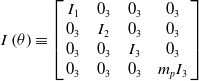 $ I\left(\theta \right)\equiv \left[\begin{array}{c@{\quad}c@{\quad}c@{\quad}c}{I}_{1}& {0}_{3} & {0}_{3}& {0}_{3} \\ {0}_{3}& {I}_{2} &{0}_{3} &{0}_{3}\\{0}_{3} &{0}_{3}& {I}_{3}& {0}_{3}\\{0}_{3}& {0}_{3} & {0}_{3}& {m}_{p}{I}_{3}\end{array}\right]$
 \begin{align*} C(\theta ,\dot{\theta })\equiv \left[\begin{array}{c@{\quad}c@{\quad}c@{\quad}c}{C}_{1}& {0}_{3}& {0}_{3}& {0}_{3}\\ \\[-7pt] {0}_{3}& {C}_{2} &{0}_{3}& {0}_{3}\\ \\[-7pt]{0}_{3} &{0}_{3}& {C}_{3} &{0}_{3}\\ \\[-7pt] {0}_{3}& {0}_{3}& {0}_{3}& {0}_{3}\end{array}\right]; \,\, \textrm{}\gamma \equiv \left[\begin{array}{c}{\gamma }_{1}\\ \\[-7pt] {\gamma }_{2}\\ \\[-7pt] \begin{array}{c}{\gamma }_{3}\\ \\[-7pt] {\gamma }_{p}\end{array}\end{array}\right]\end{align*}
 \begin{align*} J\equiv \left[\begin{array}{c@{\quad}c@{\quad}c}{J}_{1}& {0}_{3}& {0}_{3}\\ \\[-7pt] {0}_{3}& {J}_{1} &{0}_{3}\\ \\[-7pt] {0}_{3}& {0}_{3}& {J}_{1} \\ \\[-7pt] {I}_{3} & {I}_{3} & {I}_{3} \end{array}\right];\,\,\, \textrm{}\lambda \equiv \left[\begin{array}{c}{\lambda }_{1}\\ \\[-7pt] {\lambda }_{2}\\ \\[-7pt] {\lambda }_{3}\end{array}\right]\,\, {\rm and}\,\, \tau \equiv \left[\begin{array}{c}{\tau }_{1}\\ \\[-7pt] {\tau }_{2}\\ \\[-7pt] {\tau }_{3}\end{array}\right]\end{align*}
The dynamic analyses of the multibody system are required to know the trajectory of different coordinates for a given torque or for a required trajectory what should be the torque at a different degree of freedom [Reference Gupta, Chaudhary and Saha29]. The dynamic modelling of the manipulator (parallel) is essential for their control because they are preferred in an application where precise positioning is required. Combining the equations of motion yields equation 53 and is represented as
 \begin{align} &\left[\begin{array}{c@{\quad}c@{\quad}c@{\quad}c}{I}_{{1}_{3x3}}& {0}_{3x3}& 0& 0\\ \\[-11pt] 0& {I}_{2}& 0& 0\\ \\[-11pt]0& 0& {I}_{3} &0\\ \\[-11pt]0& 0 & 0& {M}_{pf}\end{array}\right]\left[\begin{array}{c}\ddot{{\theta }_{1}}\\ \\[-11pt] \begin{array}{c}\ddot{{\theta }_{2}}\\ \\[-11pt] \ddot{{\theta }_{3}}\\ \\[-11pt] \begin{array}{c}\ddot{{\theta }_{4}}\\ \\[-11pt] \ddot{{\theta }_{5}}\\ \\[-11pt] \begin{array}{c}\ddot{{\theta }_{6}}\\ \\[-11pt] \ddot{{\theta }_{7}}\\ \\[-11pt] \begin{array}{c}\ddot{{\theta }_{8}}\\ \\[-11pt] \ddot{{\theta }_{9}}\\ \\[-11pt] \begin{array}{c}\ddot{{x}_{p}}\\ \\[-11pt] \begin{array}{c}\ddot{{y}_{p}}\\ \\[-11pt] \ddot{{z}_{p}}\end{array}\end{array}\end{array}\end{array}\end{array}\end{array}\end{array}\right]+\left[\begin{array}{c@{\quad}c@{\quad}c@{\quad}c}{C}_{1}& 0&0 &0\\ \\[-11pt] 0& {C}_{2}& 0& 0\\ \\[-11pt] 0& 0& {C}_{3} &0\\ \\[-11pt] 0 &0& 0& 0\end{array}\right]+\left[\begin{array}{c}{\gamma }_{1}\\ \\[-11pt] {\gamma }_{2}\\ \\[-11pt] \begin{array}{c}{\gamma }_{3}\\ \\[-11pt] {\gamma }_{pf}\end{array}\end{array}\right] \nonumber\\[3pt] & \quad =\left[\begin{array}{c@{\quad}c@{\quad}c}{J}_{{c1}_{3x3}}^{T} &0& 0\\ \\[-11pt]0& {J}_{{c2}_{3x3}}^{T}& 0 \\ \\[-11pt]0&0&{J}_{{c3}_{3x3}}^{T}\\ \\[-11pt]{1}_{3x3}& {1}_{3x3}& {1}_{3x3}\end{array}\right]{\left[\begin{array}{c}{\lambda }_{1}x\dots z\\ \\[-11pt] {\lambda }_{2}x\dots z\\ \\[-11pt] {\lambda }_{3}x\dots z\end{array}\right]}_{9x1}+\left[\begin{array}{c}\begin{array}{c}{\tau }_{1}\\ \\[-11pt] 0\\ \\[-11pt] 0\end{array}\\ \\[-11pt] \begin{array}{c}{\tau }_{1}\\ \\[-11pt] 0\\ \\[-11pt] 0\end{array}\\ \\[-11pt] \begin{array}{c}{\tau }_{1}\\ \\[-11pt] 0\\ \\[-11pt] \begin{array}{c}0\\ \\[-11pt] 0\\ \\[-11pt] \begin{array}{c}0\\ \\[-11pt] 0\end{array}\end{array}\end{array}\end{array}\right]\end{align}
The RHS of equation 53 can also be re-written for inverse dynamics as
 \begin{align} \left[\begin{array}{c@{\quad}c@{\quad}c@{\quad}c@{\quad}c@{\quad}c@{\quad}c@{\quad}c@{\quad}c@{\quad}c@{\quad}c@{\quad}c}1& {J}_{11}& {J}_{21}&{J}_{31} &0&0&0&0&0&0&0&0\\ \\[-11pt] 0& {J}_{12}& {J}_{22}&{J}_{32}&0&0&0&0&0&0&0&0\\ \\[-11pt] 0& {J}_{13}& {J}_{23}& {J}_{33}&0&0&0&0&0&0&0&0\\ \\[-11pt] 0&0&0&0&1& {J}_{11}& {J}_{21}&{J}_{31}&0&0&0&0\\ \\[-11pt] 0&0&0&0& 0& {J}_{12}& {J}_{22}&{J}_{32}&0&0&0&0\\ \\[-11pt] 0&0&0&0& 0& {J}_{13}& {J}_{23}& {J}_{33}&0&0&0&0\\ \\[-11pt]0&0&0&0&0&0&0&0&1&{J}_{11}& {J}_{21}&{J}_{31}\\ \\[-11pt]0&0&0&0&0&0&0&0&0& {J}_{12}& {J}_{22}&{J}_{32}\\ \\[-11pt]0&0&0&0&0&0&0&0&0& {J}_{13}& {J}_{23}& {J}_{33}\\ \\[-11pt]0&1&0&0&0&1&0&0&0&1&0&0\\ \\[-11pt]0&0&1&0&0&0&1&0&0&0&1&0\\ \\[-11pt]0&0&0&1&0&0&0&1&0&0&0&1 \\ \\[-11pt] \end{array}\right]\left[\begin{array}{c}\begin{array}{c}\begin{array}{c}\begin{array}{c}\begin{array}{c}\begin{array}{c}{\tau }_{1}\\ \\[-11pt] {\lambda }_{1x}\end{array}\\ \\[-11pt] {\lambda }_{1y}\\ \\[-11pt] {\lambda }_{1z}\end{array}\\ \\[-11pt] {\tau }_{2}\\ \\[-11pt] {\lambda }_{2x}\end{array}\\ \\[-11pt] {\lambda }_{2y}\\ \\[-11pt] {\lambda }_{2z}\end{array}\\ \\[-11pt] {\tau }_{3}\\ \\[-11pt] {\lambda }_{3x}\end{array}\\ \\[-11pt] {\lambda }_{3y}\\ \\[-11pt] {\lambda }_{3z}\end{array}\right]\end{align}
4.4. Numerical illustration
This section presents the implementation of the inverse dynamics methodology for the three – DOF delta robots proposed in section IV (B).
 \begin{align*}{{\bf{J}}_{\tau k}} \equiv \left[ {\begin{array}{*{20}{c}}{{J_k}(1,3)}\\ \\[-7pt]{{J_k}(2,3)}\\ \\[-7pt]{{J_k}(3,3)}\end{array}} \right];\,{{\bf{\lambda }}_k} \equiv \left[ {\begin{array}{*{20}{c}}{{\lambda _{xk}}}\\ \\[-7pt]{{\lambda _{yk}}}\\ \\[-7pt]{{\lambda _{zk}}}\end{array}} \right]\end{align*}
Figure 10(a) shows the delta robot whose mass centre was offset to the geometric centre of the RecurDynTM model for demonstration. Referring to Fig. 10(b), each cut joint is represented by three components of the Lagrange multipliers vector
 ${\bf{\lambda }}$
, as the joints are spherical.
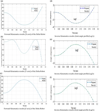
(a) Forward kinematics results [X axis] of the delta robot. (b) Forward kinematics results [Y axis] of the delta robot. (c) Forward kinematics results [Z axis] of the delta robot. (d) Inverse kinematics results (Joint angle profile (Leg1)). (e) Inverse kinematics results (joint angle profile (Leg2)). (f) Inverse kinematics results (joint angle profile (Leg3)).

In a way, there are nine components of the Lagrange multipliers to be computed due to three cut joints. Using the methodology explained in section IV (D), forces at the legs were calculated as given next.
 \begin{align}\phi _u^* \equiv \left[ {\begin{array}{*{20}{c}}{{\phi _{I1}}}\\ \\[-7pt]{{\phi _{I2}}}\\ \\[-7pt] \vdots \\ \\[-7pt]{{\phi _{VI1}}}\\ \\[-7pt]{{\phi _{VI2}}}\end{array}} \right];\,{{\bf{J}}_u} \equiv \left[ {\begin{array}{c@{\quad}c@{\quad}c@{\quad}c}{{{\bf{J}}_{Iu}}}&{\bf{O}} &\cdots& {\bf{O}}\\ \\[-7pt]{\bf{O}}&{{{\bf{J}}_{IIu}}} &\cdots &{\bf{O}}\\ \\[-7pt] \vdots & \vdots & \ddots& \vdots \\ \\[-7pt]{\bf{O}}&{\bf{O}} &\cdots &{{{\bf{J}}_{VIu}}}\end{array}} \right]\end{align}
where
 $\phi _u^*$
is the 12-dimensional vector related to unactuated joints of the legs,
 ${{\bf{J}}_u}$
is 12×18 matrix containing the elements of the Jacobian matrices associated with the unactuated joints of the legs, and
 ${\bf{O}}$
is the 2×3 matrix of zeros. The diagonal elements
 ${{\bf{J}}_u}$
have been represented using the kth subsystem as
 \begin{align*}{{\bf{J}}_{ku}} \equiv \left[ {\begin{array}{*{20}{c}}{{J_k}(1,1)}{{J_k}(2,1)}{{J_k}(3,1)}\\ \\[-7pt] {{J_k}(1,2)}{{J_k}(2,2)}{{J_k}(3,2)}\end{array}} \right]\end{align*}
5. Catching
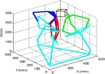
Once the intrinsic matrix [Reference Kushal, Bansal and Banerjee30,Reference Criminisi, Reid and Zisserman31] is computed for the fixed cameras, each runs in a thread. In the system, three threads run and give the pose of the cube to the fixed frame [Reference Criminisi32,Reference Wang, Tsui, Zhanyi and Wu33], as shown in Fig. 12. In each thread, communication with Matlab is performed synchronously.
Catching the free-fall cube in space.

Testing of the algorithm is performed by various trajectories such as free fall, vertical projection, and projection spatial and planar. The position estimation of the trajectories from one of the calibrated cameras is shown in section VII (F).
6. Results
6.1. Kinematics simulation results
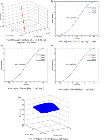
The 3D trajectories with respect to the fixed base frame of all three delta robots are shown in Fig. 13(a).
(a) The 3D trajectory of delta robot {1, 2, 3} with respect to delta frame. (b) Joint angles of Delta1 [Leg1, Leg2, Leg3]. (c) Joint angles of Delta2 [Leg1, Leg2, Leg3]. (d) Joint angles of Delta3 [Leg1, Leg2, Leg3]. (e) The workspace of Delta1 [Leg1, Leg2, Leg3].

Given the position vectors to the fixed base frame and performing the inverse kinematics resulted in the joint angles of each of the Deltas as shown in Fig. 13(b)–(d). From Fig. 13(b)–(d), each leg of the delta robot starts from 0 degrees and reaches the final point at 30 degrees.
Given the input, the joint angles and forward kinematics resulted in the position vectors to the fixed base frame of each delta, as shown in Fig. 13(e).
6.2. Kinematics results validated using RecurDyn TM
The position and joint angles plots are given in Fig. 11(a)–(f), respectively. Note that to validate the results, the kinematic analyses were carried out using the commercial software RecurDynTM. The comparison in the above figures proves the correctness of the proposed methodology.
6.3. Dynamics analysis results
The dynamic analysis performed for the straight-line trajectory, i.e., initial xi = 1.0384e-15, yi = 0.00002479, zi = 0.0878350;
 ${{\rm{P}}_1} = \left[ {\begin{array}{*{20}{c}}{{x_{\rm{i}}}}\\{{y_{\rm{i}}}}\\{{z_{\rm{i}}}}\end{array}} \right];{\rm{\;}}$
and the final xf = 1.400e-15, yf = 0.0000248, zf = 0.1828063;
 ${{\rm{P}}_2} = \left[ {\begin{array}{*{20}{c}}{{x_f}}\\{{y_{\rm{f}}}}\\{{z_{\rm{f}}}}\end{array}} \right].{\rm{\;\;}}$
Case I. [From P1 to P2]
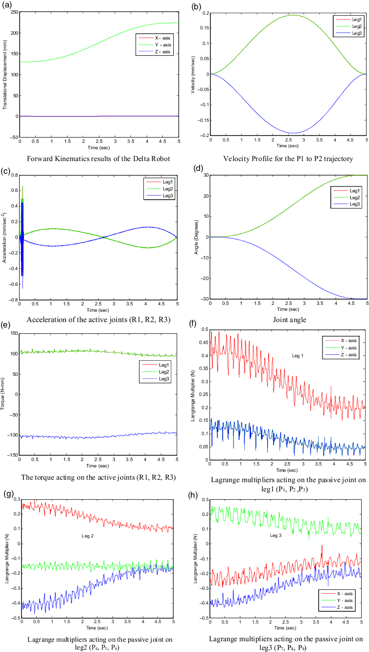
Figure 14(a)–(c) shows the position, velocity, and acceleration profile. The torque acting on the active joints (rotatory) is shown in Fig. 14(d). The torque acting on the passive joints (universal) are shown in Fig. 14(e)–(h).
(a) Forward kinematics results of the delta robot [P1 to P2]. (b) Velocity profile for the P1 to P2 trajectory. (c) Acceleration of the active joints (R1, R2, R3). (d) Joint angle. (e) The torque acting on the active joints (R1, R2, R3). (f) Lagrange multipliers acting on the passive joint on leg1 (P1, P2, P3). (g) Lagrange multipliers acting on the passive joint on leg2 (P4, P5, P6). (h) Lagrange multipliers acting on the passive joint on leg3 (P7, P8, P9).

Case II. [From P2 to P1]
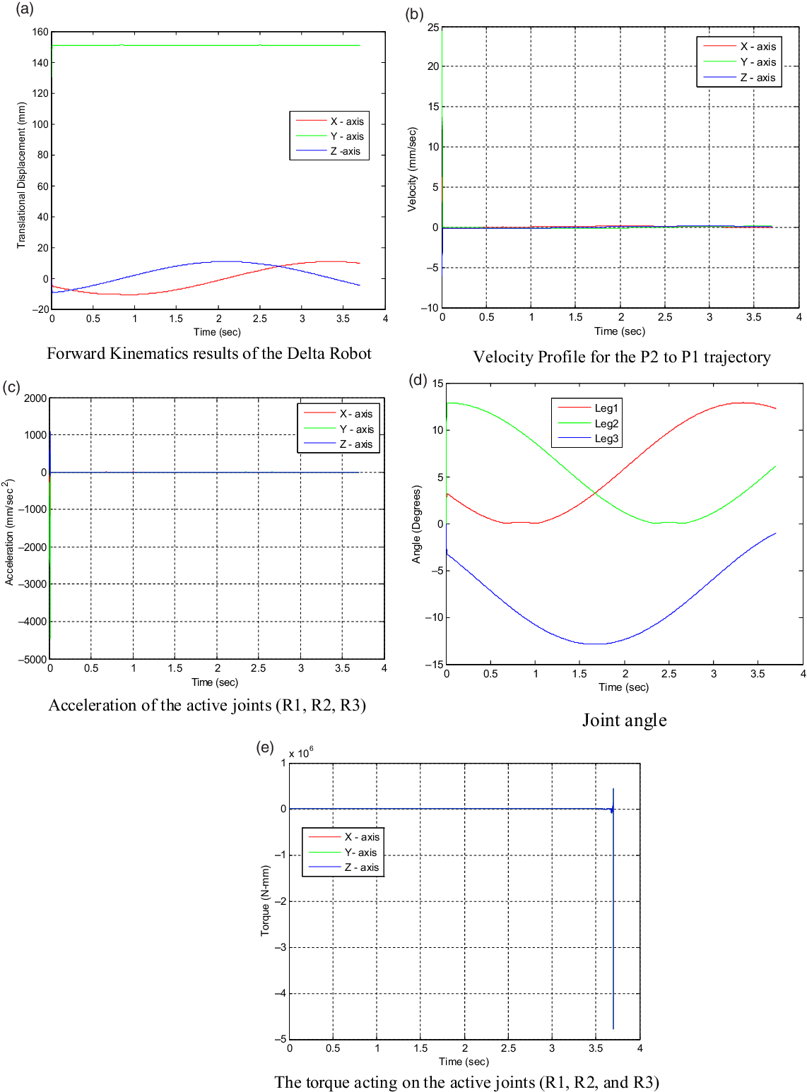
The joint angle, position, velocity, and acceleration profile are shown in Fig. 15(a)–(d). The torque acting on the active joints (rotatory) is shown in Fig. 15(e).
(a) Forward kinematics results of the delta robot [P2 to P1]. (b) Velocity profile for the P2 to P1 trajectory. (c) Acceleration of the active joints (R1, R2, R3). (d) Joint angle. (e) The torque acting on the active joints (R1, R2, R3).

Case III. Circular Trajectory
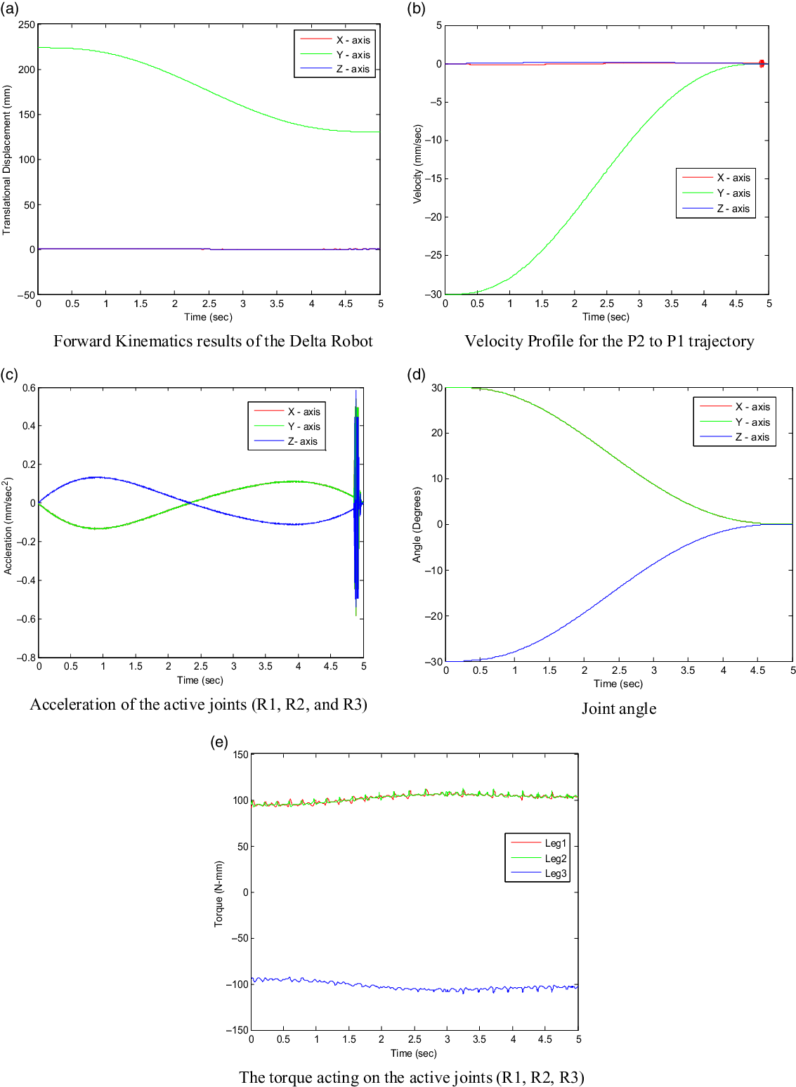
The joint angle, position, velocity, and acceleration profile are shown in Fig. 16(a)–(d). The torque acting on the active joints (rotatory) is shown in Fig. 16(e).
(a) Forward kinematics results of the delta robot [circular trajectory]. (b) Velocity profile for the P2 to P1 trajectory. (c) Acceleration of the active joints (R1, R2, R3). (d) Joint angle. (e) The torque acting on the active joints (R1, R2, R3).

Case IV. Helical Trajectory
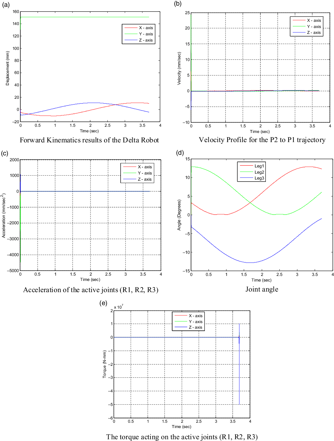
The joint angle, position, velocity, and acceleration profile are shown in Fig. 17(a)–(d). The torque acting on the active joints (rotatory) is shown in Fig. 17(e).
(a) Forward kinematics results of the delta robot [helical trajectory]. (b) Velocity profile for the P2 to P1 trajectory. (c) Acceleration of the active joints (R1, R2, R3). (d) Joint angle. (e) The torque acting on the active joints (R1, R2, R3).

6.4. Real-time controlling of the delta manipulator
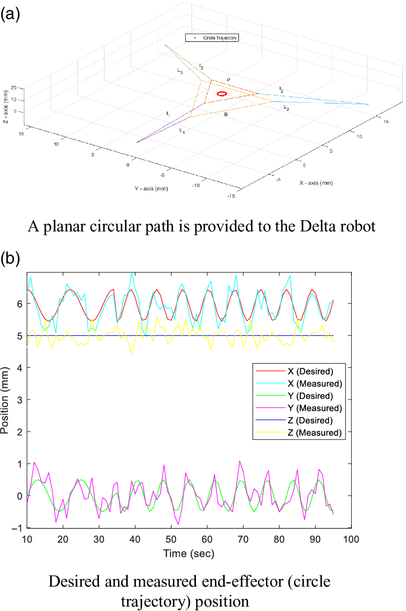
In this case, a planar circular path was input. The delta robot movement while following the path 02 times recorded by the encoders. The planar circular path is shown in Fig. 18(a).
(a) A planar circular path is provided to the delta robot. (b) Desired and measured end-effector (circle trajectory) position.

Delta robot FPK diagram.

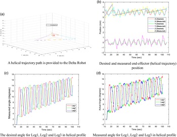
(a) A helical trajectory path is provided to the delta robot. (b) Desired and measured end-effector (helical trajectory) position. (c) The desired angle for Leg1, Leg2, and Leg3 in helical profile. (d) Measured angle for Leg1, Leg2, and Leg3 in helical profile.

In this case, a helical trajectory was given input. The delta robot movement following the path was recorded. As the helical path is provided to the delta robot, as shown in Fig. 19(a), to the inverse kinematics function and its corresponding theta angles estimated. The desired and measured end-effector (helical trajectory) position is shown in Fig. 19(b). The error in executing a circular profile is analysed. Desired angles in Leg1, Leg2 and Leg3 are shown in Fig. 19(c), and measured angles in Leg1, Leg2 and Leg3 are shown in Fig. 19(d).
I have hence tested the fundamental motions. Since the general motion of a rigid body in space is described by a screw (Chasal’s Theorem), I have also tested helical motion. I have hence validated that the error between the vision-based measurement and kinematics based on link length and encoder angles is of the order of a degree.
The result section (VI), sub-section A (kinematics simulation results), sub-section B (kinematics results validated using RecurDynTM and sub-section C (dynamics analysis results) presented the simulation-based implementation. The sub-section D (real-time controlling of the delta manipulator) presented the experimental results using the real robot(s) (delta robot).
7. Conclusion
Inthis paper, kinematic and dynamic analysis of the proposed architecture has been discussed. A description of the topological structure, geometrical model and the kinematics analysis of the three figured systems is presented. In kinematics analysis, inverse kinematics and forward kinematics solutions of the delta manipulator are implemented. The differences of the kinematics of the delta manipulator using forward kinematics based on encoders readings and the real-time vision-based system are termed as the error, and its characteristics have been investigated. The dynamic analysis was implemented using the DeNOC approach. Various cases in real time and in the virtual environment, achieving the object’s catching, have been discussed. In the future, we will implement the proposed framework to experiment with an irregular shaped object (like a semi filled bottle) with object-based classification techniques. It can be further extended by using the vision and electromechanical robot hardware in a real-time environment to demonstrate catching.
Acknowledgements
We hereby acknowledge the support of Dr. Anil Kumar Sharma for the help and Mechatronics Lab, IIT Delhi, for providing the facility and environment for carrying out the research activity.
Conflicts of Interest
None.
Financial Support
None.
Ethical Considerations
None.
Authors’ Contributions
None.