1 Introduction
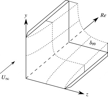
The flow along a right-angled corner formed by the intersection of two flat plates (figure 1) has been studied in the past as a generic model for various technical applications. Rubin (Reference Rubin1966) was the first to present the full set of equations for the laminar incompressible corner-flow problem based on self-similar transformation and matched asymptotic expansions. The asymptotic behaviour of the flow was further studied by Pal & Rubin (Reference Pal and Rubin1971). In vicinity of the cornerline, the boundary layer of the corner flow is three-dimensional and, due to the displacement effect of the opposing walls, a secondary cross-flow velocity exists at the far field away from the cornerline. Therefore, the far-field boundary layer is similar to the two-dimensional flat-plate scenario with additional secondary cross-flow (Rubin Reference Rubin1966; Pal & Rubin Reference Pal and Rubin1971; Ghia & Davis Reference Ghia and Davis1974). After the first numerical solution of the corner-flow equations by Rubin & Grossman (Reference Rubin and Grossman1971), far-field boundaries at true infinity were introduced (Ghia Reference Ghia1975) and the problem was extended to arbitrary angles (Barclay & Ridha Reference Barclay and Ridha1980). Ridha (Reference Ridha1992) included the streamwise pressure gradient and was the first to show the dual solution (upper and lower branch) behaviour of the flow for different wall-shear values. The effect of compressibility was first accounted for in the corner-layer equations by Weinberg & Rubin (Reference Weinberg and Rubin1972) for a model fluid with a Prandtl number of
 $\mathit{Pr}=1$
. Mikhail & Ghia (Reference Mikhail and Ghia1978) computed self-similar solutions without the restriction to unity Prandtl number. Schmidt & Rist (Reference Schmidt and Rist2011) obtained the base state as a solution to the parabolized Navier–Stokes (PNS) equations instead of solving the corner-layer equations.
For the inviscid problem, a two-dimensional temporal linear stability theory (LST) analysis of the corner flow was first performed by Balachandar & Malik (Reference Balachandar and Malik1995). Lin, Wang & Malik (Reference Lin, Wang and Malik1996) solved the viscous eigenvalue problem (EVP) based on the streamwise velocity and the pressure for a non-self-similar base flow. Parker & Balachandar (Reference Parker and Balachandar1999) studied the temporal linear stability for an incompressible corner flow of finite spanwise extent in the case of oblique modes and a pressure gradient. The obtained eigenvalue spectrum consisted of discrete Tollmien–Schlichting (TS)-wave-like viscous modes with variable spanwise wavenumbers
 $\unicode[STIX]{x1D6FD}$
and an inviscid even-symmetric corner mode. The stability behaviour of the viscous modes was found to be similar to the flat-plate scenario. The amplification rates of oblique modes with respect to
 $\unicode[STIX]{x1D6FD}$
were studied. Depending on their propagation direction, these modes were either named incoming (
 $\unicode[STIX]{x1D6FD}<0$
) or outgoing (
 $\unicode[STIX]{x1D6FD}>0$
). It was shown that the growth-rate maximum occurs for incoming modes, whereas its minimum appears for outgoing modes at a different
 $|\unicode[STIX]{x1D6FD}|$
value. This asymmetric behaviour is explained as an effect of the sidewall, which suppresses the disturbance growth of waves moving away from the cornerline and enhances the growth of modes moving towards the cornerline. A sensitivity analysis due to variations of the corner base flow was performed by Alizard, Robinet & Rist (Reference Alizard, Robinet and Rist2010).
Sketch of the flow along a streamwise corner (Schmidt & Rist Reference Schmidt and Rist2011):
 $U_{\infty }$
is the non-dimensional free-stream velocity,
 $\unicode[STIX]{x1D6FF}_{99}$
denotes the local boundary-layer thickness where
 $u=0.99$
,
 $y$
and
 $z$
are the cross-stream directions and the Reynolds number
 $\mathit{Re}$
indicates the streamwise direction.

For compressible flows at Mach numbers up to 1.5, Schmidt & Rist (Reference Schmidt and Rist2011) observed the same effects concerning oblique modes as for incompressible flows. By animating the modal structures in time, it was shown that the propagation direction of these modes was not oblique as expected but in the streamwise direction, and an alternative boundary condition for modes propagating through the corner was suggested (Schmidt Reference Schmidt2014). In this paper, modes with an oblique propagation direction through the corner instead of the previously named incoming/outgoing modes are considered for the first time in detail.
2 Base flow
In this study, the steady laminar corner base flow for the stability analysis is obtained as the self-similar solution to the PNS equations. The PNS equations are derived from the compressible Navier–Stokes equations (NSEs) assuming the streamwise gradients to be small in comparison to the cross-flow gradients, and therefore all unsteady as well as all viscous terms containing gradients in the streamwise direction are dropped (Tannehill, Anderson & Pletcher Reference Tannehill, Anderson and Pletcher1997). The asymptotic behaviour of the secondary cross-flow induced by the displacement effect is guaranteed by the combination of a homogeneous Neumann boundary condition and enforcing the asymptotic solution via a sponge zone. For a more detailed description of the base-flow calculation, see Schmidt & Rist (Reference Schmidt and Rist2011).
In the following, the superscript ‘
 $\ast$
’ labels dimensional quantities. The base flow is characterized by the Prandtl number
 $\mathit{Pr}=c_{p}^{\ast }\unicode[STIX]{x1D707}_{\infty }^{\ast }/k_{\infty }^{\ast }$
and the Mach number
 $\mathit{Ma}=u_{\infty }^{\ast }/a_{\infty }^{\ast }$
, with the heat capacity at constant pressure
 $c_{p}^{\ast }$
, the dynamic viscosity
 $\unicode[STIX]{x1D707}_{\infty }^{\ast }$
, the thermal conductivity
 $k_{\infty }^{\ast }$
, the free-stream velocity
 $u_{\infty }^{\ast }$
and the speed of sound
 $a_{\infty }^{\ast }$
. The PNS equations are made dimensionless by relating all length scales to the compressible displacement thickness
 $\unicode[STIX]{x1D6FF}_{1}^{\ast }=\int _{0}^{\infty }[1-\unicode[STIX]{x1D70C}^{\ast }u^{\ast }/(\unicode[STIX]{x1D70C}_{\infty }^{\ast }u_{\infty }^{\ast })]\,\text{d}y^{\ast }$
, the pressure to
 $\unicode[STIX]{x1D70C}_{\infty }^{\ast }u_{\infty }^{\ast 2}$
and all other quantities to their dimensional free-stream value (‘
 $\infty$
’). The Reynolds number is defined as
 $\mathit{Re}=\unicode[STIX]{x1D70C}_{\infty }^{\ast }u_{\infty }^{\ast }\unicode[STIX]{x1D6FF}_{1}^{\ast }/\unicode[STIX]{x1D707}_{\infty }^{\ast }$
. The temperature dependence of the viscosity is included by the Sutherland law, with
 $\unicode[STIX]{x1D707}_{\mathit{ref}}^{\ast }=1.735\times 10^{-5}~\text{kg}~\text{m}^{-1}~\text{s}^{-1}$
,
 $T_{\mathit{ref}}^{\ast }=280~\text{K}$
and the Sutherland constant
 $S_{1}=110.4~\text{K}$
. The ideal gas constant is given by
 $R=c_{p}^{\ast }(\unicode[STIX]{x1D6FE}-1)/\unicode[STIX]{x1D6FE}$
. The base-flow solution is obtained for the free-stream values
 $$\begin{eqnarray}\left.\begin{array}{@{}c@{}}\displaystyle Ma=0.95,\quad \mathit{Pr}=0.71,\quad \unicode[STIX]{x1D6FE}=1.4,\\ \displaystyle p_{\infty }^{\ast }=101\,325~\text{Pa},\quad T_{\infty }^{\ast }=293.15~\text{K},\quad c_{p}^{\ast }=1005\,\frac{\text{J}}{\text{kg}~\text{K}}\end{array}\right\}\end{eqnarray}$$
on a computational domain of
 $y_{\mathit{max}}=z_{\mathit{max}}=60$
with a discretization of
 $[45\times 45]$
wall-clustered Chebychev–Gauss–Lobatto points.
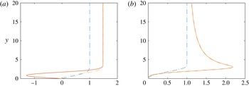
Figure 2 shows the corresponding velocity profiles. At the far field
 $z=z_{\mathit{max}}$
the streamwise velocity
 $u$
and the cross-flow velocity
 $w$
are Blasius-like and a wall-near jet evolves for the induced cross-flow velocity
 $v$
(figure 2
a). Along the corner bisector, the
 $u$
-profile displays an inflection point; the
 $v,w$
-profiles collapse and show a distinct maximum (figure 2
b).
Self-similar base-flow solution for streamwise velocity
 $u$
(– ⋅ – ⋅ –, blue) and cross-flow velocities
 $v$
(——, red),
 $w$
(– – – –, yellow) (a) at the corner far field
 $z=z_{\mathit{max}}$
and (b) along the corner bisector
 $y=z$
.

3 Linear stability
The NSEs are linearized by decomposing the flow into a steady state
 $\boldsymbol{q}_{\mathbf{0}}$
and time-varying disturbances
 $\boldsymbol{q}^{\prime }$
, and neglecting terms with products of perturbation quantities. For the perturbations
 $\boldsymbol{q}^{\prime }$
, the local two-dimensional normal mode ansatz
 $$\begin{eqnarray}\boldsymbol{q}^{\prime }(x,y,z,t)=\hat{\boldsymbol{q}}(y,z)\text{e}^{\text{i}(\unicode[STIX]{x1D6FC}x-\unicode[STIX]{x1D714}t)},\quad \unicode[STIX]{x1D6FC}\in \mathbb{R},\,\unicode[STIX]{x1D714}\in \mathbb{C}\end{eqnarray}$$
is chosen. Insertion of (3.1) into the linearized NSEs and recasting of the equations leads to the generalized EVP
 $$\begin{eqnarray}({\mathcal{A}}-\unicode[STIX]{x1D714}{\mathcal{B}})\hat{\boldsymbol{q}}=0.\end{eqnarray}$$
The boundary conditions for the EVP (3.2) are
 $\hat{u} =\hat{v}={\hat{w}}=\hat{T}=0$
at the corner walls
 $y=0$
and
 $z=0$
. Parker & Balachandar (Reference Parker and Balachandar1999) introduced the far-field boundary conditions
 $$\begin{eqnarray}\frac{\unicode[STIX]{x2202}\hat{\boldsymbol{q}}}{\unicode[STIX]{x2202}y}=\text{i}\unicode[STIX]{x1D6FD}\hat{\boldsymbol{q}}\quad \text{at}~y=y_{max}\quad \text{and}\quad \frac{\unicode[STIX]{x2202}\hat{\boldsymbol{q}}}{\unicode[STIX]{x2202}z}=\text{i}\unicode[STIX]{x1D6FD}\hat{\boldsymbol{q}}\quad \text{at}~z=z_{max}\end{eqnarray}$$
for oblique incoming/outgoing modes based on Sommerfeld’s radiation condition. Application of this boundary condition in all previous work has led to some peculiarities. Depending on the sign of the chosen
 $\unicode[STIX]{x1D6FD}$
, waves either enter
 $(\unicode[STIX]{x1D6FD}<0)$
or leave
 $(\unicode[STIX]{x1D6FD}>0)$
the integration domain at both lateral boundaries. Due to the inherent symmetry in both cases, a wave pattern occurs which travels downstream along the
 $x$
axis in the near-corner region. The resulting wave pattern itself is either symmetric or antisymmetric with respect to the corner bisector depending on the relative phase of the waves at the lateral boundaries (in phase or out of phase respectively). Amplification of this wave pattern exhibits a characteristic dependence on the wavenumber
 $\unicode[STIX]{x1D6FD}$
: a peak occurs for negative
 $\unicode[STIX]{x1D6FD}$
, i.e. for waves that run towards the corner from both sides, and a shallow minimum for the opposite
 $\unicode[STIX]{x1D6FD}>0$
, i.e. when the waves leave the corner region in positive lateral directions. Accordingly, there is no symmetry of amplification with respect to the spanwise wavenumber, which would be expected for a single wave or a wave pattern due to superposition of a left- and a right-running wave. An obvious deficiency of the boundary condition (3.3) is that it does not permit a single wave that enters the domain on one side and leaves it on the other side. However, as suggested by Schmidt (Reference Schmidt2014), this is easily obtained by setting
 $$\begin{eqnarray}\frac{\unicode[STIX]{x2202}\hat{\boldsymbol{q}}}{\unicode[STIX]{x2202}y}=\text{i}\unicode[STIX]{x1D6FD}\hat{\boldsymbol{q}}\quad \text{at}~y=y_{max}\quad \text{and}\quad \frac{\unicode[STIX]{x2202}\hat{\boldsymbol{q}}}{\unicode[STIX]{x2202}z}=-\text{i}\unicode[STIX]{x1D6FD}\hat{\boldsymbol{q}}\quad \text{at}~z=z_{max}.\end{eqnarray}$$
The computational grid domain for the eigenvalue calculation is set to
 $y_{\mathit{max}}=z_{\mathit{max}}=45$
and discretized by [
 $90\times 90$
] grid points as a result of a convergence study with
 $\unicode[STIX]{x1D6FD}=0$
,
 $y_{\mathit{max}}=z_{\mathit{max}}\in [35,55]$
and
 $N\in [45,115]$
. To guarantee a higher grid-point clustering in the vicinity of the walls, an equidistant grid
 ${\hat{y}}$
is scaled by the tanh transformation
 $y=(-\tanh (-(b-a){\hat{y}}/y_{\mathit{max}}-a)-\tanh a)y_{\mathit{max}}/(\tanh b-\tanh a)$
, with
 $a=-1.8$
and
 $b=0.5$
. The self-similar base-flow results are interpolated onto the grid for the respective
 $\mathit{Re}$
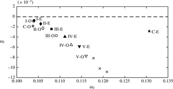
of interest. The exemplary eigenvalue spectrum shown in figure 3 for
 $\unicode[STIX]{x1D6FD}=0$
,
 $\mathit{Re}=660$
and
 $\unicode[STIX]{x1D6FC}=0.245$
is a solution to the EVP (3.2) calculated with a shift-and-invert Arnoldi method. The modes named C-O/-E are the two inviscid odd (O)-/even (E)-symmetric corner modes. The viscous TS-like modes are labelled I-/II-/… according to their respective number of spanwise
 $|\text{Re}(\hat{u} )|$
maxima. The corresponding spanwise wavelengths of the calculated viscous TS-like modes change with varying spanwise extent of the corner. By increasing
 $y_{\mathit{max}}=z_{\mathit{max}}$
, a quadratic convergence of the respective growth rates towards an asymptotic value can be detected (Parker & Balachandar Reference Parker and Balachandar1999).
Part of the eigenvalue spectrum for
 $\unicode[STIX]{x1D6FD}=0$
,
 $\unicode[STIX]{x1D6FC}=0.245$
and
 $\mathit{Re}=660$
. Filled symbols indicate even-symmetric modes and open symbols indicate odd-symmetric modes.

4 Results
To investigate the differences between the modes obtained by the suggested boundary condition for oblique modes (3.4) and the so far considered oblique incoming/outgoing modes resulting from the boundary condition (3.3) (Parker & Balachandar Reference Parker and Balachandar1999; Galionis & Hall Reference Galionis and Hall2005; Schmidt & Rist Reference Schmidt and Rist2011), the latter are calculated as well.
4.1 Stability behaviour
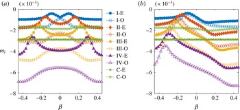
Figure 4 depicts the dependence of the temporal amplification rate
 $\unicode[STIX]{x1D714}_{i}$
on
 $\unicode[STIX]{x1D6FD}$
for the viscous modes I-E/-O to IV-E/-O and the two inviscid corner modes C-E/-O at
 $\mathit{Re}=660$
and
 $\unicode[STIX]{x1D6FC}=0.245$
. As expected, the amplification for the suggested boundary condition is perfectly symmetric with respect to
 $\unicode[STIX]{x1D6FD}=0$
(figure 4
a). Two maxima at non-zero
 $\unicode[STIX]{x1D6FD}$
-values exist for the viscous even-symmetric modes, whereas, considering viscous odd-symmetric modes, the maximum growth rate occurs for the boundary condition
 $\unicode[STIX]{x1D6FD}=0$
. In contrast to this, the asymmetric behaviour occurring in the case of incoming/outgoing modes (3.3) displays a distinct maximum for incoming modes and a faint minimum for outgoing modes (figure 4
b).
Dependence of the modal growth rate
 $\unicode[STIX]{x1D714}_{i}$
on the spanwise wavenumber
 $\unicode[STIX]{x1D6FD}$
for
 $\unicode[STIX]{x1D6FC}=0.245$
,
 $\mathit{Re}=660$
with (a) boundary condition (3.4) for modes travelling through the corner and (b) boundary condition (3.3) for incoming/outgoing modes.

Comparison of maximum growth rates
 $\unicode[STIX]{x1D714}_{i}$
and their respective
 $\unicode[STIX]{x1D6FD}$
-values for modes I-E/-O to IV-E/-O. Filled symbols denote even-symmetric modes and open symbols odd-symmetric modes, as in figure 3, for modes travelling through the corner (——) and incoming/outgoing modes (– ⋅ – ⋅ –).

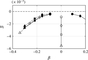
Figure 5 depicts the distribution of the growth-rate maximum of the modes I-E/-O to IV-E/-O (peaks in figure 4) with respect to their corresponding
 $\unicode[STIX]{x1D6FD}$
-values for both boundary conditions. For modes travelling through the corner as well as for incoming/outgoing modes, the even-symmetric mode of every mode pair reaches higher amplification rates (figures 4, 5; solid symbols) than the respective odd-symmetric mode (open symbols). The maximum amplification rates
 $\unicode[STIX]{x1D714}_{i,\mathit{max}}$
of the even-symmetric modes appear for both boundary conditions at the same
 $\unicode[STIX]{x1D6FD}$
-value (figure 5). This congruence of
 $\unicode[STIX]{x1D6FD}(\unicode[STIX]{x1D714}_{i,\mathit{max}})$
is apparently caused by the fact that the maximum growth rates of these modes are reached whenever the spanwise wavenumber is compatible with the
 $\unicode[STIX]{x1D6FD}$
-value set for the boundary condition, and therefore the mode is able to propagate smoothly out of or into the computational domain.
Additionally, figure 5 reveals that the actual
 $\unicode[STIX]{x1D714}_{i,\mathit{max}}$
value is slightly higher for the incoming modes (– ⋅ – ⋅ –; solid symbols) than for those travelling through the corner (——; solid symbols). A clear difference between the growth-rate behaviour occurs for the odd-symmetric modes (figure 5, open symbols); as mentioned above, those resulting from the EVP solution with the suggested boundary condition show their maximum growth rate for
 $\unicode[STIX]{x1D6FD}=0$
, whereas the respective modes for the old boundary condition reach a higher distinct maximum
 $\unicode[STIX]{x1D714}_{i}$
for
 $\unicode[STIX]{x1D6FD}<0$
(incoming). The modes for
 $\unicode[STIX]{x1D6FD}=0$
lead to a special wave pattern of standing waves as they do not enter or leave the computational domain through the lateral ends and therefore propagate strictly in the streamwise direction with fixed nodal points. Therefore, the odd-symmetric modes resulting from the new boundary condition are maximally amplified for
 $\unicode[STIX]{x1D6FD}=0$
, as travelling through the corner with
 $\unicode[STIX]{x1D6FD}\neq 0$
is not possible due to zero disturbance at the corner bisector (figure 6
b,d,e).
For the new boundary condition, increasing
 $y_{\mathit{max}}$
and
 $z_{\mathit{max}}$
has an influence on the respective spanwise wavelengths of the viscous modes I-E/O, II-E/O, III-E/O,
 $\ldots .$
The maximal amplification rate
 $\unicode[STIX]{x1D714}_{i,\mathit{max}}$
for these modes is, as expected, reached at a different matching
 $\unicode[STIX]{x1D6FD}$
-value, but the resulting datapoints
 $\unicode[STIX]{x1D714}_{i,\mathit{max}}$
are in line with the course shown in figure 5. The decrease/increase in maximum/minimum growth rate as mentioned by Parker & Balachandar (Reference Parker and Balachandar1999) for the old boundary condition in the case of increasing spanwise extent could not be observed for the new boundary condition.
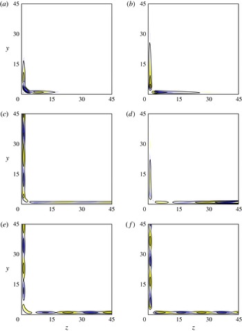
As the spanwise extent of the inviscid modes is restricted to the vicinity of the corner, they are weakly (C-O) or not (C-E) affected by the spanwise wavenumber in the case of both boundary conditions (figure 4). The weak distortion of the growth rate occurring for mode C-O is because its spanwise extent is larger than the spanwise extent of mode C-E (figure 6
a,b). By enlarging the computational domain, the influence of the far-field boundary condition on mode C-O, and therefore its
 $\unicode[STIX]{x1D6FD}$
-dependence, vanishes.
The asymmetric isocontours of the eigenfields
 $\text{Re}(\hat{u} )$
for the modes IV-E and IV-O depicted in figure 6(c,d) lead to the conclusion that the labels even- and odd-symmetric are not suitable for oblique modes obtained by the suggested boundary condition (3.4). Nevertheless, the mentioned labelling will be maintained for convenience, and, in the following, modes named …-E are modes that show an extremum at the corner bisector (figure 6
c), and those named …-O are the respective modes without an extremum at the corner bisector (figure 6
d). However, these two asymmetric modes reach their respective maximum
 $\text{Re}(\hat{u} )$
at opposing plates. For the even-symmetric mode, the distribution of the extrema along
 $y$
(figure 6
c) is similar to the distribution of the even-symmetric incoming mode (figure 6
e). The eigenfields for the modes IV-E/-O obtained by the boundary condition for incoming/outgoing modes are clearly even-/odd-symmetric to the corner bisector (figure 6
e,f), and their shape for non-zero
 $\unicode[STIX]{x1D6FD}$
-values is similar to the eigenfield of the results for
 $\unicode[STIX]{x1D6FD}=0$
.
Isocontours of the eigenfield
 $\text{Re}(\hat{u} )$
and respective isolines
 $|\hat{u} |$
(——) for
 $\unicode[STIX]{x1D6FC}=0.245$
and
 $\mathit{Re}=660$
, shown in yellow for
 $\text{Re}(\hat{u} )<0$
and blue for
 $\text{Re}(\hat{u} )>0$
. Inviscid corner modes for
 $\unicode[STIX]{x1D6FD}=0$
: (a) C-E, (b) C-O. Viscous modes for
 $\unicode[STIX]{x1D6FD}=-0.3$
corresponding to maximum growth rate: travelling through the corner (c) IV-E, (d) IV-O; incoming (e) IV-E, (f) IV-O.

4.2 Mode propagation direction
To illustrate the propagation direction of the aforementioned modes, the temporal evolution of the locations of maximum and minimum as well as zero
 $\text{Re}(\hat{u} )$
-values is depicted in figure 7 for the time interval
 $t\,\unicode[STIX]{x1D714}_{r}/2\unicode[STIX]{x03C0}\in [0,3]$
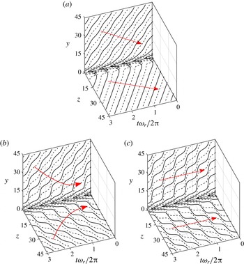
. The propagation directions at the upper and lower walls are schematically indicated by red arrows. As already mentioned by Schmidt (Reference Schmidt2014), the mode IV-E obtained with the suggested boundary condition (3.4) for
 $\unicode[STIX]{x1D6FD}=-0.3$
propagates obliquely through the corner (figure 7
a). At the lower wall, where the mode is travelling away from the corner, straight wavefronts with a constant phase angle
 $\unicode[STIX]{x1D711}=\tan ^{-1}(\unicode[STIX]{x1D6FD}/\unicode[STIX]{x1D6FC})$
are observed for
 $z>5$
. In contrast, a slightly variable phase angle is identified at the opposing wall for
 $y>5$
, where the mode is propagating towards the corner. These undulated wavefronts are due to a partial reflection of the mode at the corner with zero phase shift. The reflection superposes with the mode at the upper wall and results in the observed wavefront pattern.
Lines of temporal evolution of
 $\text{Re}(\hat{u} )$
extrema (– ⋅ – ⋅ –) and
 $\text{Re}(\hat{u} )=0$
(——) for
 $t\,\unicode[STIX]{x1D714}_{r}/2\unicode[STIX]{x03C0}\in [0,3]$
,
 $\unicode[STIX]{x1D6FC}=0.245$
,
 $\mathit{Re}=660$
and
 $\unicode[STIX]{x1D6FD}=-0.3$
at
 $y\in [1,45]$
,
 $z=1$
and
 $y=1$
,
 $z\in [1,45]$
in the case of mode IV-E (a) travelling through the corner (3.4), (b) obtained as incoming by (3.3) and (c) as linear superposition of (a) with its counterpart obtained by
 $\unicode[STIX]{x1D6FD}=0.3$
. The propagation direction in each case is schematically indicated by arrows.

For comparison, the respective temporal evolution for the incoming mode IV-E obtained by (3.3) is shown in figure 7(b). The previously mentioned symmetrical behaviour of the incoming mode is clearly visible. The propagation direction of the incoming mode changes from oblique at the lateral ends to strictly streamwise in the vicinity of the corner, which can explain the fact that the mode vanishes in the near-corner region. The slightly oblique wavefronts in the far field are similar to those at the upper wall in figure 7(a), but at a spanwise distance of 7–30 from the cornerline the wavefronts change into a step-like structure. The imposed symmetrical boundary condition (
 $\unicode[STIX]{x1D6FD}<0$
at both lateral ends) prevents the respective incoming mode from travelling through the corner and leaving through the opposite lateral end. Therefore, closer to the cornerline, the mode travels in a chequerboard-like pattern in the streamwise direction (figure 7
b). This leads to the suggestion that the incoming and outgoing modes can be reproduced by superposition of two modes travelling through the corner with mirrored wavevectors (
 $\unicode[STIX]{x1D6FD}_{1}=-\unicode[STIX]{x1D6FD}_{2}$
) and a phase shift of
 $\unicode[STIX]{x03C0}$
or no phase shift (Schmidt Reference Schmidt2014). The outgoing modes are assumed to not be physical, as they require infinite disturbance production in the near-corner region, as otherwise they would die out.
The superposition of two LST modes with
 $\unicode[STIX]{x1D6FC}_{1}=\unicode[STIX]{x1D6FC}_{2}$
and
 $\unicode[STIX]{x1D714}_{1}=\unicode[STIX]{x1D714}_{2}$
yields a mode with the same growth rate
 $\unicode[STIX]{x1D714}_{i}=\unicode[STIX]{x1D714}_{i,1}=\unicode[STIX]{x1D714}_{i,2}$
as the superposed modes. Hence, the only modes that could be a result of superposition are the even-symmetric incoming modes. It appears that the superposition with a phase shift of
 $\unicode[STIX]{x03C0}$
yields an eigenfield similar to the odd-symmetric incoming mode. However, the behaviour of the maximum growth rates of the odd-symmetric modes travelling through the corner and the respective incoming modes deviates significantly (§ 4.1). Therefore, the aforementioned superposition with a phase shift of
 $\unicode[STIX]{x03C0}$
is not further considered.
Figure 7(c) displays the temporal evolution of the mode obtained by superposition of mode IV-E shown in figure 7(a) with its mirrored counterpart and no phase shift. Close to the cornerline, the resemblance between the superposed mode and the incoming mode concerning the temporal evolution is obvious (figure 7 b,c), whereby the chequerboard-like structure is more distinct over the whole spanwise extent in the case of the superposed mode than for the incoming mode. It seems as if, in the far field, the incoming mode fulfils the oblique wave direction imprinted by the boundary condition, whereas the superposed mode pattern propagates strictly into the streamwise direction.
Superposition of one outgoing and one incoming even-symmetric mode with the same
 $\unicode[STIX]{x1D6FD}$
-value results in a similar chequerboard-like pattern to the aforementioned superposition of two single modes travelling through the corner. However, there exists no unique growth rate for the superposed disturbance, and the superposition will change with
 $t$
as the amplification rates for the incoming mode and the outgoing mode differ.
5 Conclusion
The differences concerning stability behaviour and propagation direction between the eigenmodes obtained by the so far used boundary condition (3.3) for oblique modes and those yielded by the boundary condition (3.4) suggested by Schmidt (Reference Schmidt2014) as well as a linear superposition of the latter – without phase shift and mirrored at the corner bisector – are investigated. The computed modes fulfil the expectation of wavefronts travelling obliquely through the corner and an amplification-rate
 $\unicode[STIX]{x1D6FD}$
-dependence that is symmetrical to
 $\unicode[STIX]{x1D6FD}=0$
. In contrast to incoming/outgoing modes, the maximum growth rate for viscous modes travelling through the corner is only
 $\unicode[STIX]{x1D6FD}$
-dependent for those modes labelled even-symmetric, as the maximum growth rate for modes marked odd-symmetric appears at
 $\unicode[STIX]{x1D6FD}=0$
due to zero disturbance amplification at the corner bisector for the odd-symmetric modes, whereas the amplification rates for inviscid corner modes are independent of the spanwise wavenumber
 $\unicode[STIX]{x1D6FD}$
.
Although the superposition of two oblique modes travelling through the corner leads to an eigenfield that resembles the respective even-symmetric incoming mode obtained by the old boundary condition, the result is not exactly the same. The growth rate of the superposed mode is equal to that of the underlying single mode, whereas the incoming mode has a slightly higher amplification rate due to an eigenvalue shift caused by the boundary condition. The odd-symmetric incoming/outgoing modes cannot be reproduced by superposing a single mode travelling through the corner with its counterpart, as the respective eigenvalues differ from those of the odd-symmetric modes obtained by the suggested boundary condition.
It is shown that the boundary condition suggested by Schmidt (Reference Schmidt2014) results in a flow pattern that is expected: instead of even-/odd-symmetric modes that travel either strictly towards or away from the corner, single modes propagating through the corner can be observed.