1 Introduction
Nanofluidics, the study of flows down to the nanoscale, has emerged over recent years thanks in particular to the development of new methods to fabricate controlled fluidic systems with nanoscale geometries, as well as of proper instrumentation to quantify transport at these scales (Bocquet & Tabeling Reference Bocquet and Tabeling2014). This has allowed the study of ionic and water transport across nanopores and nanotubes made of various materials, thereby revealing a number of exotic transport properties (Siria et al. Reference Siria, Poncharal, Biance, Fulcrand, Blase, Purcell and Bocquet2013; Geng et al. Reference Geng, Kim, Zhang, Escalada, Tunuguntla, Comolli, Allen, Shnyrova, Cho and Munoz2014; Joshi et al. Reference Joshi, Carbone, Wang, Kravets, Su, Grigorieva, Wu, Geim and Nair2014; Park & Jung Reference Park and Jung2014; Feng et al. Reference Feng, Graf, Liu, Ovchinnikov, Dumcenco, Heiranian, Nandigana, Aluru, Kis and Radenovic2016; Secchi et al. Reference Secchi, Marbach, Nigues, Siria and Bocquet2016). This opens up new possibilities in the development of innovative processes for desalination, nano-filtration and energy harvesting (Werber, Osuji & Elimelech Reference Werber, Osuji and Elimelech2016). However, while measurement of electrical properties across nanochannels is now relatively standard (Branton et al. Reference Branton, Deamer, Marziali, Bayley, Benner, Butler, Di Ventra, Garaj, Hibbs and Huang2008; Siria et al. Reference Siria, Poncharal, Biance, Fulcrand, Blase, Purcell and Bocquet2013; Stein Reference Stein2015; Feng et al. Reference Feng, Graf, Liu, Ovchinnikov, Dumcenco, Heiranian, Nandigana, Aluru, Kis and Radenovic2016), measurement of mass flow through nanoscale capillaries remains a considerable challenge due to the minute flow emerging from such nanopipes (Bocquet & Tabeling Reference Bocquet and Tabeling2014; Secchi et al. Reference Secchi, Nigues, Jubin, Siria and Bocquet2016). In this context, it was demonstrated recently that the peculiarities of the nanojet flow emerging from a nanocapillary, the so-called Landau–Squire flow, could be harnessed in order to reach the proper sensitivity to extract the mass transport across a tube down to nanometric sizes (Secchi et al. Reference Secchi, Marbach, Nigues, Siria and Bocquet2016).
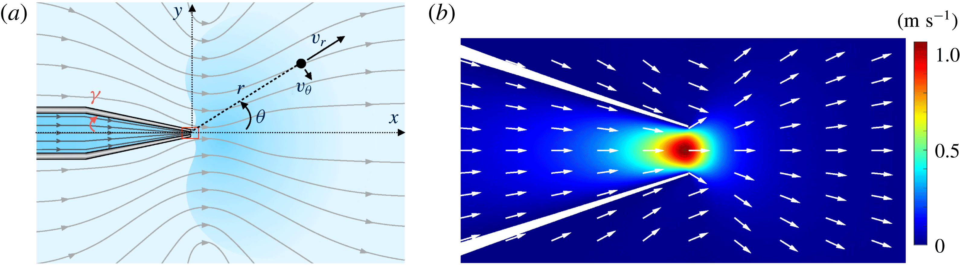
The Landau–Squire flow corresponds to a jet flow emerging from the end of a (semi-infinite) narrow tube into a reservoir with infinite dimension; see figure 1. This flow was first solved by Landau and Squire in two seminal works (Squire Reference Squire1951; Landau & Lifshitz Reference Landau and Lifshitz1959). Its properties were investigated experimentally in recent contributions by Laohakunakorn et al. (Reference Laohakunakorn, Gollnick, Moreno-Herrero, Aarts, Dullens, Ghosal and Keyser2013) and Secchi et al. (Reference Secchi, Marbach, Nigues, Siria and Bocquet2016). An interesting and peculiar specificity of this flow is that it is completely characterized by the rate of momentum transferred from the tube into the reservoir, i.e. a force – but not by the flow rate. In the viscous (low-Reynolds) regime, the solution for the flow induced in the reservoir is indeed given by a Stokeslet,
 $$\begin{eqnarray}v_{r}=\frac{F_{P}}{4\unicode[STIX]{x03C0}\unicode[STIX]{x1D702}}\frac{\cos \unicode[STIX]{x1D703}}{r},\quad v_{\unicode[STIX]{x1D703}}=-\frac{F_{P}}{8\unicode[STIX]{x03C0}\unicode[STIX]{x1D702}}\frac{\sin \unicode[STIX]{x1D703}}{r},\end{eqnarray}$$
where the tube tip is taken as the origin for the distance
 $r$
and the angle
 $\unicode[STIX]{x1D703}$
is measured from the tube axis;
 $\unicode[STIX]{x1D702}$
is the fluid viscosity (figure 1). In this equation,
 $F_{P}$
has the dimension of a force and corresponds to the fluid momentum transfer. On dimensional grounds, the jet force
 $F_{P}$
is accordingly expected to take the form of a Stokes formula in the viscous regime (Secchi et al.
Reference Secchi, Marbach, Nigues, Siria and Bocquet2016),
 $$\begin{eqnarray}F_{P}=\unicode[STIX]{x1D6FC}\unicode[STIX]{x1D702}R_{1}\overline{v},\end{eqnarray}$$
where
 $R_{1}$
is the characteristic radial dimension of the tube and
 $\overline{v}$
is the average flow velocity emerging from the tube tip, defined in terms of the fluid flux
 $Q$
as
 $\overline{v}=Q/\unicode[STIX]{x03C0}R_{1}^{2}$
;
 $\unicode[STIX]{x1D6FC}=O(1)$
is a numerical coefficient which depends on the specific geometry of the tip of the nanocapillary. A quantitative estimate of
 $\unicode[STIX]{x1D6FC}$
can be obtained numerically (Secchi et al.
Reference Secchi, Marbach, Nigues, Siria and Bocquet2016).
Landau–Squire jet flow emerging from a nanocapillary. (a) Schematic of pressure-driven streamlines inside the nanocapillary and Landau–Squire streamlines outside; the angle
 $\unicode[STIX]{x1D6FE}$
defines the internal half-opening-angle of the nanocapillary. (b) Close-up view of red box in (a); simulated flow amplitude at the nanocapillary tip (box size
 $1.25~\unicode[STIX]{x03BC}\text{m}\times 2.5~\unicode[STIX]{x03BC}\text{m}$
; nanocapillary tip diameter 250 nm).

In this paper, we consider a situation in which a dye is added to the capillary and dispersed into the reservoir from the capillary tip under the application of a pressure drop. A stationary plume is created in the reservoir, the shape of which results from the competition between the convection under the Landau–Squire pressure-driven flow and the molecular diffusion of the dye. In the following, we first solve analytically the convection–diffusion equation for the dye concentration in the reservoir (§ 2); and then compare the results with an experimental investigation of the plume of a fluorescent dye dispersed from nanocapillaries (§ 3).
2 The Landau–Squire plume: theoretical predictions
We show here that the dispersion of dye particles via the Landau–Squire (LS) flow field can be predicted analytically. We consider a situation in which the flowing fluid inside the capillary is seeded with a dye, with concentration
 $C_{0}$
and bulk diffusion coefficient
 $D$
. The dye emerges into the reservoirs from the tip of the feeding capillary, which therefore acts as a point source with, say, an incoming solute flux
 $\unicode[STIX]{x1D6F7}_{0}$
. The latter is the sum of a convective contribution,
 $QC_{0}$
, and a diffusive contribution proportional to
 ${\sim}R_{1}DC_{0}$
(with a prefactor whose explicit expression, which depends on the geometry of the seeding capillary tip, will not be needed in the following). Due to the infinite volume of the reservoir, a steady state is reached and the stationary concentration of particles verifies the diffusion–convection equation,
 $$\begin{eqnarray}D\unicode[STIX]{x0394}C-\boldsymbol{v}\boldsymbol{\cdot }\unicode[STIX]{x1D735}C=0,\end{eqnarray}$$
where
 $\boldsymbol{v}(\boldsymbol{r})$
is the Landau–Squire (divergence-free) flow field in the reservoir in (1.1). In spherical coordinates, equation (2.1) reads
 $$\begin{eqnarray}D\frac{1}{r^{2}}\unicode[STIX]{x2202}_{r}(r^{2}\unicode[STIX]{x2202}_{r}C)+D\frac{1}{r^{2}\sin \unicode[STIX]{x1D703}}\unicode[STIX]{x2202}_{\unicode[STIX]{x1D703}}(\sin \unicode[STIX]{x1D703}\unicode[STIX]{x2202}_{\unicode[STIX]{x1D703}}C)-\frac{F_{p}}{4\unicode[STIX]{x03C0}\unicode[STIX]{x1D702}r}\cos \unicode[STIX]{x1D703}\unicode[STIX]{x2202}_{r}C+\frac{F_{p}}{8\unicode[STIX]{x03C0}\unicode[STIX]{x1D702}r}\frac{\sin \unicode[STIX]{x1D703}}{r}\unicode[STIX]{x2202}_{\unicode[STIX]{x1D703}}C=0.\end{eqnarray}$$
We first note that any function of the type
 $f(\unicode[STIX]{x1D703})/r^{n}$
, with
 $n$
a real number, can be a solution of (2.2). However, conservation of the number of dye particles imposes that for any
 $r$
,
 $$\begin{eqnarray}\unicode[STIX]{x1D6F7}_{0}=2\unicode[STIX]{x03C0}r^{2}\int _{\unicode[STIX]{x1D703}=0}^{\unicode[STIX]{x03C0}}J_{r}(r,\unicode[STIX]{x1D703})\sin \unicode[STIX]{x1D703}\,\text{d}\unicode[STIX]{x1D703},\end{eqnarray}$$
where
 $J_{r}(r,\unicode[STIX]{x1D703})=-D\unicode[STIX]{x2202}_{r}C+(F_{p}\cos \unicode[STIX]{x1D703}/4\unicode[STIX]{x03C0}\unicode[STIX]{x1D702}r)C$
is the radial component of the particle flux and
 $\unicode[STIX]{x1D6F7}_{0}$
is the total solute flux. This imposes
 $n=1$
, and we deduce
 $C(r,\unicode[STIX]{x1D703})=f(\unicode[STIX]{x1D703})/r$
. The differential equation for
 $f(\unicode[STIX]{x1D703})$
takes the form
 $$\begin{eqnarray}D\sin \unicode[STIX]{x1D703}\unicode[STIX]{x2202}_{\unicode[STIX]{x1D703}}(\sin \unicode[STIX]{x1D703}\unicode[STIX]{x2202}_{\unicode[STIX]{x1D703}}f)+\frac{F_{p}}{4\unicode[STIX]{x03C0}\unicode[STIX]{x1D702}}\cos \unicode[STIX]{x1D703}f+\frac{F_{p}}{8\unicode[STIX]{x03C0}\unicode[STIX]{x1D702}}\sin \unicode[STIX]{x1D703}\unicode[STIX]{x2202}_{\unicode[STIX]{x1D703}}\,f=0.\end{eqnarray}$$
The general solution of this equation is obtained as
 $$\begin{eqnarray}f(\unicode[STIX]{x1D703})=A\text{e}^{(Pe/2)\cos \unicode[STIX]{x1D703}}+B\text{e}^{(Pe/2)(\cos \unicode[STIX]{x1D703}-1)}\left\{-\text{e}^{Pe}\int _{-(Pe/2)(\cos \unicode[STIX]{x1D703}+1)}^{\infty }\frac{\text{e}^{-t}}{t}\,\text{d}t+\int _{(Pe/2)(1-\cos \unicode[STIX]{x1D703})}^{\infty }\frac{\text{e}^{-t}}{t}\,\text{d}t\right\},\end{eqnarray}$$
where
 $A$
and
 $B$
are two integration constants. This solution introduces an effective Péclet number specific to the Landau–Squire problem and defined as
 $$\begin{eqnarray}Pe=\frac{F_{p}}{4\unicode[STIX]{x03C0}\unicode[STIX]{x1D702}D}.\end{eqnarray}$$
Imposing that
 $f$
is a regular function yields
 $B=0$
, and
 $A$
is deduced from solute number conservation, equation (2.3). Altogether, the solution of the diffusion–convection problem thus reads
 $$\begin{eqnarray}C(r,\unicode[STIX]{x1D703})=\frac{\unicode[STIX]{x1D6F7}_{0}}{4\unicode[STIX]{x03C0}Dr}(1+\unicode[STIX]{x1D700}(Pe))\text{e}^{(Pe/2)(\cos \unicode[STIX]{x1D703}-1)},\end{eqnarray}$$
where
 $\unicode[STIX]{x1D700}(Pe)=(1-(1+Pe)\text{e}^{-Pe})/(Pe-1+(1+Pe)\text{e}^{-Pe})$
is a small contribution of
 $Pe$
(vanishing for low and high
 $Pe$
and always smaller than 0.5).
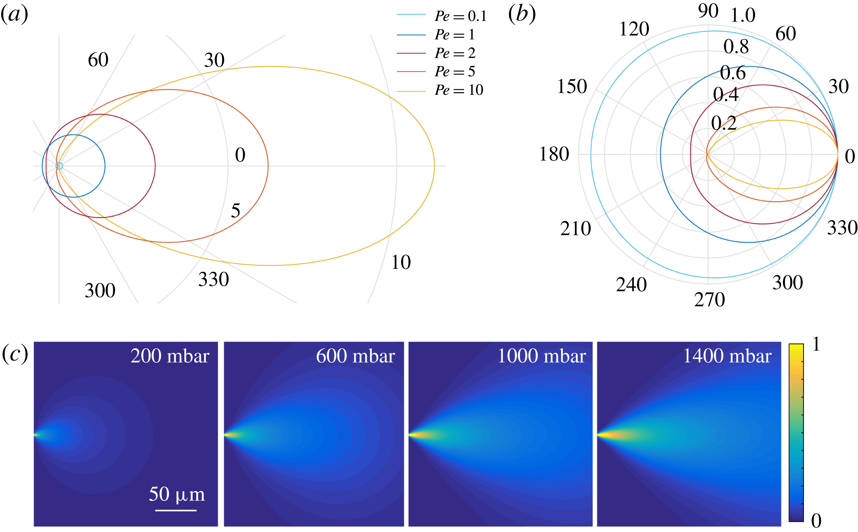
The shape of the plume-like concentration profile for different Péclet numbers. (a) Iso-concentration profiles derived from
 $r/r_{c}=Pe\,\text{e}^{(Pe/2)(\cos \unicode[STIX]{x1D703}-1)}$
, with
 $r_{c}$
a characteristic length scale independent of
 $Pe$
, for different Péclet numbers (for illustration, we assumed
 $\unicode[STIX]{x1D6F7}_{0}\propto Pe$
). (b) Renormalized iso-concentration profiles
 $r/r_{max}=\text{e}^{(Pe/2)(\cos \unicode[STIX]{x1D703}-1)}$
for several Péclet numbers. For small
 $Pe$
, the profile is very circular, nearly diffusive. For large
 $Pe$
, the profile is severely distorted in a plume-like shape by the Landau–Squire flow. The colour scale is the same for both plots. (c) Simulated concentration profiles in the
 $x,y$
plane, divided by the largest concentration value measured, for a nanocapillary with dimensions
 $R_{1}=120~\text{nm}$
and
 $\unicode[STIX]{x1D6FE}=4^{\circ }$
.

This shows that the concentration profile exhibits an interesting combination of a long-range
 $1/r$
power-law decay (its amplitude
 $\unicode[STIX]{x1D6F7}_{0}$
being linearly dependent on the flow
 $Q$
, see above), with an exponential dependence of the azimuthal shape on the Landau–Squire jet force
 $F_{p}$
via
 $Pe$
. Typical concentration profiles are shown in figure 2(a,b). We show for illustration a numerical calculation of the full concentration profile evolution with increasing pressure drop in figure 2(c). The latter is obtained by combining a finite-element solver for the LS flow following Secchi et al. (Reference Secchi, Marbach, Nigues, Siria and Bocquet2016) and a finite-difference solver for the concentration profile in (2.1).
The general properties of the plume as observed in figure 2(a), namely the shape and aspect ratio, can be predicted from (2.7). For low Péclet number, the profile is isotropic (circular shape) with an aspect ratio close to unity. For large Péclet number, the concentration profile in (2.7) simplifies to
 $C(r,\unicode[STIX]{x1D703})=(\unicode[STIX]{x1D6F7}_{0}/4\unicode[STIX]{x03C0}Dr)\exp [-(Pe/4)\unicode[STIX]{x1D703}^{2}]$
, so that the aspect ratio of the plume is accordingly expected to scale sublinearly with the Péclet number, as
 $1/\overline{\unicode[STIX]{x1D703}}\sim Pe^{1/2}$
for
 $Pe\gg 1$
.
3 Experimental investigation of the Landau–Squire flow emerging from a glass nanocapillary
We now turn to an experimental study of the dispersion of a fluorescent dye emerging from a glass nanocapillary.
3.1 Experimental set-up and procedure
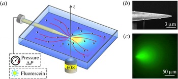
The experimental set-up is sketched in figure 3. The cell was composed of two macroscopic reservoirs bridged by a nanocapillary. A pressure drop was imposed on the (sealed) reservoir located at the rear, while the front reservoir was kept at ambient pressure. It was constituted of two glass slides, in order to allow visualization of the region in front of the nanocapillary tip. The glass slides were separated by a plastic frame, sealed via two Viton joints (of thickness 0.125 mm) and squeezed between the upper and lower parts of the chamber. The pressure was controlled by an AF1 microfluidic pressure pump from Elveflow.
Sketch of the experimental set-up. (a) Sketch of the experimental set-up for the optical detection of the dye plume emerging from the nanocapillary, and imaging of the flow field via particle tracking of colloids. (b) Scanning electron microscope image of a typical glass nanocapillary. (c) The fluorescence signal emitted from fluorescein at 1.5 mM emerging from a nanocapillary with
 $R_{1}=120$
nm and
 $\unicode[STIX]{x1D6FE}=3^{\circ }$
at
 $\unicode[STIX]{x0394}P=1550~\text{mbar}$
.

Nanocapillaries were fabricated on the basis of pulled Pasteur pipettes. Glass capillaries were purchased from Sutter Instrument Company (standard wall borosilicate tubing, internal diameter 0.5 mm, external diameter 1 mm and length 10 cm) and were pulled using a programmable laser puller (P-2000 laser-based microcapillary puller, Sutter Instrument Company). The parameters of the capillary puller were finely tuned in order to fix the outer geometry of the nanocapillary tip and vary the dimension of the opening. The nanopore radius was measured with a scanning electron microscope (SEM, Nova Nanosem). The typical shape of a pulled nanocapillary is presented by the SEM image of the tip in figure 3(b).
Fluorescein (Sigma Aldrich) was dispersed in deionized water to a final concentration of 1.5 mM. NaOH was added to the deionized water to reach a pH equal to 8. The water was previously degassed and filtered with syringe filters with
 $0.2~\unicode[STIX]{x03BC}\text{m}$
pore size. The glass nanocapillaries were air-plasma treated for 5 min in a low-power plasma cleaner (Harrick Plasma) and immediately filled with the fluorescein solution. The nanocapillary was inserted into the holder and the cell was sealed. The glass reservoir was rinsed with deionized water. For the tracking experiments to characterize the LS flow, the reservoir was filled with a suspension of polystyrene particles (diameter
 $0.5~\unicode[STIX]{x03BC}\text{m}$
, Biovalley) at a volume fraction of
 $\unicode[STIX]{x1D719}=10^{-5}$
at
 $\text{pH}=8$
.
The experimental set-up was mounted on the stage of an inverted optical microscope equipped with epifluorescence (Olympus IX71 equipped with a
 $60\times$
long working distance objective). The particle tracking experiment was performed in bright-field configuration, while the fluorescein was imaged in epifluorescence configuration with an exposure of 200 ms. A constant pressure was applied to the reservoir at the rear of the capillary for a time interval varying from 1 to 10 min. Flow movies were recorded with a CMOS camera (Orca-Flash V 4.0, Hamamatsu, 16 bit,
 $2024\times 2024$
pixels,
 $6.5\times 6.5~\unicode[STIX]{x03BC}\text{m}$
in size). For the particle tracking experiments, a typical run consisted of 8000–12 000 images, acquired with a frame rate of 200–320 f.p.s. and an exposure time of 1.5–3 ms. The procedure was repeated for several pressure values, varying from 20 to 1700 mbar, depending on the dimensions of the glass nanopore. For the plume imaging experiments, the frame rate was lower (typically 0.7 f.p.s.) due to the longer exposure (200 ms). A typical fluorescence plume is shown in figure 3(c).
3.2 Landau–Squire flow data analysis
Before exploring the fluorescent plume systematically, we first fully characterized the Landau–Squire flow in the reservoir. This was investigated with a standard velocimetry technique, using the polystyrene particles as colloid tracers. This follows the approach described in Secchi et al. (Reference Secchi, Marbach, Nigues, Siria and Bocquet2016), and details of the experimental and numerical analysis may be found in the supplementary material of this reference. We recall briefly the method and outline the main results.
A region in front of the nanocapillary tip with dimensions
 $(\text{d}x,\text{d}y)=(45,90)~\unicode[STIX]{x03BC}\text{m}$
is selected. Image analysis is performed by in-house particle tracking algorithms. The optics has a depth of field comparable to the particle dimension and the algorithm analyses only the particles in focus. This allows the plane to be set at
 $z=0$
, and the distance from the nanocapillary tip is
 $r=\sqrt{x^{2}+y^{2}}$
. In this configuration, we obtain all the information on the 3D velocity field by analysing the 2D
 $x{-}y$
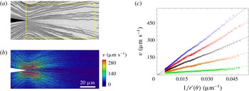
plane passing through the centre of symmetry of the nanocapillary tip. We show in figure 4(a,b) a typical example for particle tracking, tracer trajectories, and corresponding velocities.
Velocimetry measurements of Landau–Squire jet flow. (a) Tracer trajectories outside a nanocapillary at
 $\unicode[STIX]{x0394}P=140$
mbar, revealing a Landau–Squire jet flow. The dashed box highlights the region where image analysis is performed. (b) Velocity fields at
 $\unicode[STIX]{x0394}P=140$
mbar. All data are obtained with a nanocapillary with
 $R_{1}=200$
nm and
 $\unicode[STIX]{x1D6FE}=9.7^{\circ }$
. (c) Particle velocity as a function of the position-dependent parameter
 $r^{\prime }(\unicode[STIX]{x1D703})=r\times 2/\sqrt{1+3\cos ^{2}\unicode[STIX]{x1D703}}$
for various values of
 $\unicode[STIX]{x0394}P$
. From bottom to top,
 $\unicode[STIX]{x0394}P=20$
, 60, 100, 140 and 180 mbar. Here, the nanocapillary geometry is
 $R_{1}=320$
nm and
 $\unicode[STIX]{x1D6FE}=12^{\circ }$
. Continuous lines are fits using
 $v=F_{P}/(4\unicode[STIX]{x03C0}\unicode[STIX]{x1D702})\times 1/r^{\prime }$
, allowing estimation of
 $F_{P}/4\unicode[STIX]{x03C0}\unicode[STIX]{x1D702}$
.

The particle tracking algorithm provides, for each particle, its position
 $(x,y)$
and velocity components,
 $v_{x}(x,y)$
and
 $v_{y}(x,y)$
. The Landau–Squire theory predicts
 $v=\sqrt{v_{r}^{2}+v_{\unicode[STIX]{x1D703}}^{2}}=(F_{P}/4\unicode[STIX]{x03C0}\unicode[STIX]{x1D702})(1/r^{\prime }(\unicode[STIX]{x1D703}))$
, with
 $r^{\prime }(\unicode[STIX]{x1D703})=r\times 2/\sqrt{1+3\cos ^{2}\unicode[STIX]{x1D703}}$
. Accordingly, for each position
 $(x,y)$
, we calculate
 $r^{\prime }(\unicode[STIX]{x1D703})$
and the velocity modulus
 $v$
. We repeat the procedure for all of the trajectories. As shown in figure 4(c), a linear relation between
 $v$
and
 $1/r^{\prime }$
is measured, as expected from the Landau–Squire theory. The slope of the lines allows the jet force
 $F_{P}/4\unicode[STIX]{x03C0}\unicode[STIX]{x1D702}$
to be extracted.
From these experiments, we deduce the pressure dependence of the jet force
 $F_{P}$
for a given nanocapillary. The several runs performed at each pressure allow us to check the stability of the flow during time. As an ultimate check, we also vary the dimensions of the analysed area
 $(\text{d}x,\text{d}y)$
, in order to ensure that it does not impact the estimation of
 $F_{P}$
. As a final note, it is also possible to analyse the flow in the plane
 $(x,y,z)=(0,y,z)$
, accounting for the 3D nature of the hydrodynamic problem, and we find results in agreement with the Landau–Squire flow.
We finally note that once the
 $F_{P}$
parameter is known for a given pressure
 $\unicode[STIX]{x0394}P$
, the flow rate
 $Q$
can be deduced thanks to a proper calibration of
 $\unicode[STIX]{x1D6FC}$
, via (1.2). This follows the approach introduced in Secchi et al. (Reference Secchi, Marbach, Nigues, Siria and Bocquet2016), where details can be found in the supplementary material. We show, in particular, that
 $\unicode[STIX]{x1D6FC}$
depends only on the opening angle
 $\unicode[STIX]{x1D6FE}$
of the nanocapillary:
 $\unicode[STIX]{x1D6FC}$
is a decreasing function of the angle
 $\unicode[STIX]{x1D6FE}$
and vanishes as the opening angle
 $\unicode[STIX]{x1D6FE}$
reaches
 $90^{\circ }$
. We find that in the region of aperture angles
 $\unicode[STIX]{x1D6FE}$
used in the experiments, the value of
 $\unicode[STIX]{x1D6FC}$
varies between 0.7 and 1.0. However, once the geometry is known for a given nanocapillary (e.g. by SEM imaging), the value of
 $\unicode[STIX]{x1D6FC}$
can be quantitatively predicted for this specific geometry with a 5 % indetermination; see the supplementary material in Secchi et al. (Reference Secchi, Marbach, Nigues, Siria and Bocquet2016).
3.3 Dispersion by the Landau–Squire flow field
We now turn to the main question of this paper and investigate the dispersion of the fluorescein solution by the LS flow field. Once a pressure drop
 $\unicode[STIX]{x0394}P$
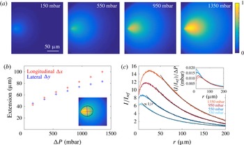
is established, a steady state is reached within a few seconds. We checked separately that at these concentrations, the fluorescence intensity maps may be directly correlated to the concentration map of fluorescein and bleaching does not affect our results. We show in figure 5(a) the evolution of the intensity signal at steady state with increasing pressure
 $\unicode[STIX]{x0394}P$
. The cloud of dispersing fluorescein is clearly distorted into a plume-like shape as the pressure increases, or equivalently as the Péclet number increases. A striking point is that the plume is observed to extend over hundreds of microns, three orders of magnitude larger than the typical nanocapillary aperture, with measurable asymmetry over very long length scales. This is quantified in figure 5(b), where the extension of the plume in both the longitudinal (
 $\unicode[STIX]{x0394}x$
) and lateral (
 $\unicode[STIX]{x0394}y$
) directions is plotted for various pressure drops, reaching
 $100~\unicode[STIX]{x03BC}\text{m}$
in the present conditions, while the nanocapillary aperture is 120 nm in this case. Here, the plume extension is obtained experimentally from an iso-intensity threshold, defined as the line where the detected intensity is half of the maximum intensity; see the red line in the inset of figure 5(b). In more detail, we plot in figure 5(c) the spatial evolution of the fluorescence intensity along the longitudinal axis in front of the nanocapillary (here normalized by a reference value
 $I_{ref}$
in the absence of fluorescence). This is shown to exhibit a long-range decay, which is well fitted by the predicted
 $1/r$
spatial relaxation in the far field, according to (2.7) for
 $\unicode[STIX]{x1D703}=0$
. Furthermore, its amplitude is shown to scale with the pressure drop
 $\unicode[STIX]{x0394}P$
, as highlighted in the inset of figure 5(c). The discrepancy at short distances, with a non-monotonic dependence of the intensity, may be attributed to non-trivial point spread dispersion of the optical set-up, which we did not explore exhaustively in this paper.
Experimental fluorescence profiles with increasing pressure drop. (a) Normalized fluorescence maps emerging from a nanocapillary in a deionized water reservoir at pH8, for increasing pressure drop
 $\unicode[STIX]{x0394}P$
. The intensity is normalized by the largest pixel intensity measured. The radius of the nanocapillary is
 $R_{1}=120~\text{nm}$
and its opening angle is
 $\unicode[STIX]{x1D6FE}=3^{\circ }$
. (b) Longitudinal
 $\unicode[STIX]{x0394}x$
and lateral
 $\unicode[STIX]{x0394}y$
extension of the plume as a function of the pressure drop, defined as the longitudinal and lateral extensions (respectively red and blue lines in the inset) of the iso-intensity profile (black line) at maximum intensity of a given map over 2. (c) Intensity on the centre horizontal line in front of the nanocapillary for increasing pressure drop as a function of the distance
 $r$
from the nanocapillary tip. The solid lines are
 $1/r$
fits. The inset shows the same profiles renormalized by the pressure drop.

Going further, more quantitative information on the flow can be obtained from the detailed shape of the iso-intensity lines. Indeed, according to the theoretical prediction in (2.7), the shape of an iso-intensity line is expected to verify
 $$\begin{eqnarray}r(\unicode[STIX]{x1D703})=r_{max}\times \exp \left[\frac{Pe}{2}(\cos \unicode[STIX]{x1D703}-1)\right],\end{eqnarray}$$
with
 $Pe=F_{p}/4\unicode[STIX]{x03C0}\unicode[STIX]{x1D702}D$
the Péclet number and
 $r_{max}$
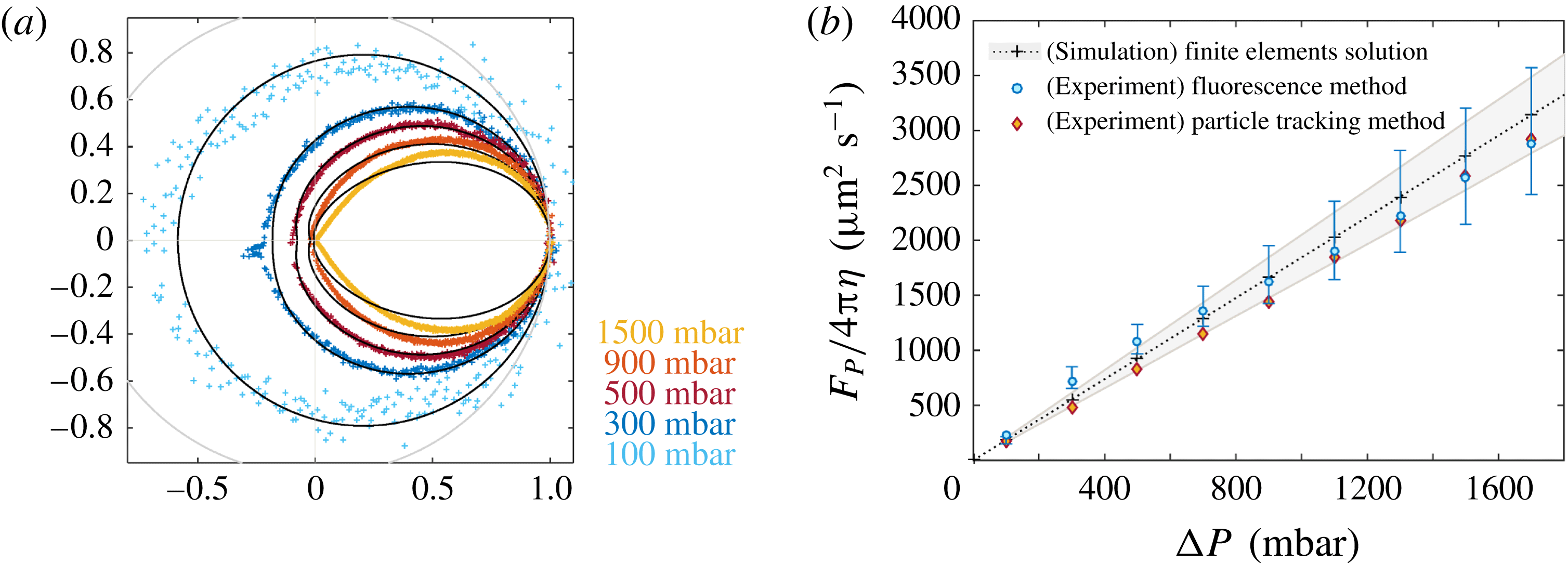
the maximal extension. In figure 6(a), we accordingly fit the normalized shape
 $r(\unicode[STIX]{x1D703})/r_{max}$
for various pressure drops using this expression. As shown in figure 6(a), the profiles are well described by the theoretical prediction using the Péclet number as a single parameter for each pressure drop. Interestingly, the back-diffusion of the plume shape for
 $\unicode[STIX]{x1D703}=\unicode[STIX]{x03C0}$
is shown to vary strongly with the pressure drop, in particular for small
 $\unicode[STIX]{x0394}P$
; see figure 6(a). This is in full agreement with the prediction
 $r(\unicode[STIX]{x1D703}=\unicode[STIX]{x03C0})/r_{max}=\exp [-Pe]$
in (3.1). Back-diffusion provides, therefore, a sensitive probe of the Péclet number, in particular for low
 $Pe$
.
Experimental plume shapes and Péclet number. (a) Normalized iso-intensity profiles with increasing pressure drop (coloured dots). The profiles are fitted according to the theoretical prediction with
 $Pe$
as the only fitting parameter (nanocapillary with
 $R_{1}=115~\text{nm}$
and
 $\unicode[STIX]{x1D6FE}=3^{\circ }$
). The grey line is the unit circle. (b) The LS force parameter
 $F_{p}/4\unicode[STIX]{x03C0}\unicode[STIX]{x1D702}=D\times Pe$
for the same nanocapillary, measured from both fluorescence and velocimetry techniques plotted versus the pressure drop
 $\unicode[STIX]{x0394}P$
. For the fluorescence technique,
 $F_{P}$
is deduced from the values of the Péclet number extracted from the fluorescence profiles in (a). For the velocimetry approach, it is extracted from the analysis of the LS flow, as in figure 4. We also report the results obtained from a finite-element calculation (crosses). The shaded area corresponds to a
 $0.5^{\circ }$
uncertainty on
 $\unicode[STIX]{x1D6FE}$
. The error bars on the fluorescence technique are defined by the variability according to different iso-intensity values.

In figure 6(b), we then plot the extracted LS force
 $F_{p}/4\unicode[STIX]{x03C0}\unicode[STIX]{x1D702}=D\times Pe$
as a function of the pressure drop
 $\unicode[STIX]{x0394}P$
, showing an expected linear dependence on pressure drop (for small pressure drop);
 $D$
is the fluorescein diffusion coefficient (
 $D=425~\unicode[STIX]{x03BC}\text{m}^{2}~\text{s}^{-1}$
(Culbertson, Jacobson & Ramsey Reference Culbertson, Jacobson and Ramsey2002)). To assess these results, we compare the pressure dependence of the LS force
 $F_{p}$
with alternative measurements obtained from the direct tracking of colloidal particles; see § 3.2. The comparison between the two shows a very good agreement; see figure 6(b). For completeness, we also compare these values with the Stokes prediction in (1.2), with the parameter
 $\unicode[STIX]{x1D6FC}$
obtained from numerical finite-element calculation for the nanocapillary geometry under consideration. The latter was obtained along the same lines as in Secchi et al. (Reference Secchi, Marbach, Nigues, Siria and Bocquet2016), supplementary material. We emphasize that no fitting parameter is used to compute this estimate.
All three estimates are found to be in very good agreement, confirming that the fluorescence measurement is a proper tool to extract flow information in this Landau–Squire geometry.
4 Summary and concluding remarks
In this paper, we have explored experimentally and theoretically the plume generated by a dye dispersed from a jet flow emerging from the tip of a nanocapillary into a large reservoir, here named the Landau–Squire plume. We have analytically predicted and experimentally assessed the solute concentration profile in the form
 $C(r,\unicode[STIX]{x1D703})\sim 1/r\times \text{e}^{(Pe/2)(\cos \unicode[STIX]{x1D703}-1)}$
, where
 $Pe=F_{p}/4\unicode[STIX]{x03C0}\unicode[STIX]{x1D702}D$
is the Péclet number associated with the Landau–Squire flow. A key remark is that
 $Pe$
depends only on the flow characteristics inside the tube, since
 $Pe\propto R_{1}\overline{v}/D$
is defined in terms of the (nanoscale) tube properties, with
 $\overline{v}$
the averaged flow inside the tube with radius
 $R_{1}$
.
The concentration profile thus combines a long-range
 $1/r$
power-law decay – with an amplitude linear in the flow rate
 $Q$
– with an exponential dependence of the azimuthal plume shape on the Péclet number
 $Pe$
. This contrasted dependence makes the shape of the dye plume very sensitive to the flow occurring inside the tube, while being measurable at very long distances from the tip, much longer than the characteristic tip size. This point is particularly obvious in figure 5, where the asymmetric plume extends over hundreds of microns, three orders of magnitude larger than the typical nanocapillary aperture. In practice, a useful remark is that the back-diffusion of the plume shape (for
 $\unicode[STIX]{x1D703}=\unicode[STIX]{x03C0}$
) is exponentially dependent on the Péclet number and thus constitutes a sensitive measurement of
 $Pe$
, in particular for low Péclet number. Altogether, the Landau–Squire plume bridges the gap between the nanoscale tube flow and the micron scales at which it can be easily characterized.
This feature is a key asset for the measurement of ultra-small flow rates occurring in nanoscale pipes thanks to the dye plume properties. Indeed, the criterion of detectability via the plume is that the Péclet number, which, we emphasize, is defined in terms of inner tube flow properties, is larger than unity. This criterion is much less stringent than direct velocimetry inside the nanochannel and is definitely reachable even for tubes with diameters in the range of nanometres (and even more for tubes that exhibit surface slippage such as carbon nanotubes; see Secchi et al. Reference Secchi, Marbach, Nigues, Siria and Bocquet2016).
Provided that they are successfully attached to the tip of the nanocapillary, the flow through various nanoporous systems can be investigated using analysis of the plume they generate, from small nanotubes to biology-inspired nanosystems like porins. Moreover, other sources of driving, like electro-osmosis or diffusio-osmosis, can also be explored using the same technique. The Landau–Squire plume is a powerful and versatile tool for nanofluidics.
Acknowledgements
We thank D. Stein and U. Keyser for fruitful discussions. E.S., A.N., S.M. and A.S. acknowledge funding from the European Union’s H2020 Framework Programme/ERC Starting Grant agreement number 637748 – NanoSOFT. S.M. acknowledges funding from a J.-P. Aguilar grant. We acknowledge funding from ANR project BlueEnergy.