2.1. Economics without Econometrics

The first powerfully expressed “LSE approach” was actually that enunciated by Lionel Robbins. Robbins (1932) claimed that economic theory provided general, formal explanations that were applicable always and everywhere that resource allocation impinged. Since the assumptions of economics were “self-evidently true” and the logic impeccable, the conclusions must be correct. However, such insights as economics delivered could not be given quantitative expression, since causes were nonuniform over both time and space. Robbins argued, therefore, that statistical relationships in economics would change when the world did, so the discipline could never boast “statistical laws” like the natural sciences (see, e.g., Hendry and Morgan, 1995). Robbins's general approach was later supported at the LSE by the work of Friedrich von Hayek (Hayek, 1963). More recently, some “freshwater” economists in the United States seem to be the inheritors of the Robbins tradition (see, e.g., Kydland and Prescott, 1991, 1996).

In principle, economic theory could indeed apply even when there were no quantitative laws, although such explanations would be somewhat unsatisfactory—like predicting calm seas as the norm after a storm, to borrow from Keynes. Moreover, Robbins's positive argument for the power of economic theory explanations only becomes a negative one for econometrics on substantiating the claim that useful empirical regularities do not exist (see, e.g., Hendry, 1995a). Certainly, Dr. Blank's nebulous demand function for herrings could only last the test of time if many factors other than price and income were included in his model, but such additional factors are not precluded a priori. Indeed, when Hutchison (1938) launched his critical attack on Robbins, he made a similar argument and proposed instead a move toward “positive economics,” a theme we resume in the next section (for the background to the general arguments, see, e.g., Blaug, 1980). Nevertheless, since Robbins was one of LSE's most eminent economists, the LSE might seem an unpromising location for a group of econometricians, particularly one with an interest in econometric methodology.

2.2. Positive Economics

However, the postwar period saw a strong move within LSE economics toward implementing a “positivist” philosophical standpoint (for an explanation of the variants of “positivism” see, e.g., Caldwell, 1982). The LSE itself had a strong tradition in the philosophy of science centered on Karl Popper, later supported by others such as Imre Lakatos (see, e.g., Popper, 1959, 1963; Lakatos, 1974). Thus, “falsification” was much under discussion at the LSE.

In economics, activity focused on the Staff Seminar on Methodology, Measurement and Testing (M²T), whose members included Chris Archibald, Kurt Klappholz, and Richard Lipsey, all of whom published on economic methodology (see, e.g., Archibald, 1959; Klappholz and Agassi, 1959; Lipsey, 1966). Here, for example, the famous Phillips curve was first presented and discussed (Phillips, 1958; see, e.g., Holt, 1969). The appointment of an engineer-economist like A.W.H. (Bill) Phillips, who stressed empirical evidence, signaled that the mood was less inimical to econometric modeling as the route ahead for economics than the heritage of Robbins might suggest. Indeed, important antecedents were already in place. Both Bill Phillips and Rex Bergstrom (also then at LSE) considered models that were essentially equilibrium-adjustment mechanisms (see, e.g., Phillips, 1954, 1957; and also Bergstrom, 1962, 1967; and the implementation in Bergstrom and Wymer, 1976).²

In any case, Denis Sargan was first appointed in the Statistics Department at the LSE in 1963, where Roy Allen played a major role. Allen admired Phillips's earlier work on control theory (Phillips, 1954, 1957), and he included an explanation of integral, derivative, and proportional control in his textbook (Allen, 1963, Ch. 9). This strand also recurs subsequently, especially in Section 3.2.

2.3. The Sargan “Revolution”

Denis himself was a somewhat unlikely candidate to revolutionize econometric methodology. His initial research had been on mathematical economics, followed by econometric theory, particularly seeking to establish the same form of rigorous inferential basis for its application to small samples that Student's famous t-distribution paper had done for statistics (see Student, 1908). Indeed, the majority of his publications were to be in what he called “advanced econometric theory” (see Sargan, 1988b).

However, prior to his arrival at the LSE in 1963, Denis had written two papers on empirical modeling issues, published as Sargan (1957) and Sargan (1964). The former points to his later role in developing methodology; the latter provided several major advances therein.

Sargan (1957) was a discussion of the pathbreaking analysis of the Oxford Savings Survey by Malcolm Fisher (1956).³

Sargan (1964), which was to become perhaps his most famous paper, was prepared for the Colston Society conference on National Economic Planning held at Bristol University in 1963 (for an appraisal of its impact, see, e.g., Desai et al., 1997). The next section considers that paper in more detail, emphasizing that almost every aspect of the current “LSE approach” was present.

3.1. Long-Run Economic Theory

The substantive problem that Denis addressed was empirical modeling of wages and prices (described in more detail in Section 3.10). Previous models had considered the changes in the variables, namely, wage and price inflation. Consider a conditional bivariate model of a variable denoted y_t (the log of wages, say) given another variable z_t (the log of prices), written in first differences as

Assuming that

and that the differenced variables are stationary with means

, then the long-run steady-state solution to (1) is

As formulated, (1) does not establish any relationship between the levels y_t and z_t; hence they could drift apart. Denis argued that economic agents would be concerned about the level of real wages, namely, y_t − z_t, not just price inflation. Thus, he formulated a model with a long-run levels equilibrium, denoted (y − z)_e,t and given by

where x_t denotes a vector of additional variables, such as unemployment, real productivity, and political factors. A unit coefficient on productivity would make the wage share a component of the left-hand side, but in practice, productivity was approximated by a linear deterministic trend in his wage models.

The disequilibrium is given by

In modern parlance, the levels are

when the differences are

. Consequently, if such a relation as (3) did exist, it would require that v_t was

and so entail that y_t was cointegrated with z_t and x_t (see, among many others, Engle and Granger, 1987; Phillips and Loretan, 1991; Banerjee, Dolado, Galbraith, and Hendry, 1993).

3.2. Equilibrium-Correction Mechanisms

Some of the antecedents to the formulation of equilibrium-correction mechanisms were noted in Section 2.2; Section 3.11 comments on the terminology. If (2) is to be the long-run equilibrium, then a mechanism is needed in (1) to reestablish the relationship between the levels of y_t, z_t, and x_t whenever they drift apart. To achieve (2), Denis postulated the explicit adjustment equation,

equivalent to including v_t−1 from (3) in (1). Doing so unrestrictedly then entails adding the levels terms (y − z)_t−1 and x_t−1. When contemporaneous variables are excluded, the resulting equation is

Consequently, when π₃ ≠ 0, the long-run levels equilibrium solution to (5) becomes

matching (2).

The model in (5) has both derivative and proportional control (e.g., Δz_t−1 and (y − z)_t−1), following up Phillips (1954, 1957) (see Salmon, 1982). The latter mechanism also ensures the disequilibrium adjustment, based on the (detrended) log-ratio of two nominal levels (see Bergstrom, 1962). Although Denis formulated (5) without specifying any specific integration properties for the data, the long-run relative stability of the “great ratios” in Klein (1953) was implicitly assumed to justify such transformations (see, e.g., the discussion of Granger and Newbold, 1977, in Hendry, 1977). Granger (1981) related the type of model in (5) to cointegration, and Granger (1986) showed that one of Δy_t or Δz_t must then depend on the equilibrium correction: the assumption in (4) is that y_t adjusts to the disequilibrium. If both variables y_t and z_t adjust to the disequilibrium, then z_t is not weakly exogenous for the {π_i} (see Phillips and Loretan, 1991; Hendry, 1995b). It is primarily because of cointegration that equilibrium-correction models like (5) have proved a popular specification.

His empirical model is described in more detail in Section 3.10, but an interesting feature of his two main equations for wages and prices, respectively, was that they had different long-run solutions. Thus, although the integrability of data derives from a reduced-rank condition (fewer corrections than variables; see, e.g., Johansen, 1988), the existence of equilibrium corrections in his two main equations by itself did not preclude that the data were

around a deterministic trend. Alternatively, the variables could have been

by inheriting unit roots from either import prices (from the price equation) or productivity (wage equation).

3.3. Autoregressive Errors

Prior to Denis's Colston paper, it was common in econometrics to test for residual autocorrelation (e.g., by the Durbin and Watson statistic; see Durbin and Watson, 1950, 1951), and if such was found, to estimate an autoregressive-error process (see Cochrane and Orcutt, 1949). Thus, autoregressive errors were viewed as a “generalization” of white-noise errors. Denis showed that autoregressive errors were a restriction on a more general dynamic model that, when valid, allowed a more parsimonious representation, thereby reversing the conventional interpretation. Further developments on this topic are taken up in Section 4.

3.4. Misspecification Tests

Denis stressed that empirical specifications should be stringently evaluated. Drawing on Sargan (1961), he formulated a test for the validity of the instrumental variables used in estimation and derived its distribution under the null. He estimated an autoregressive-error process for each equation by least squares or instrumental variables. To evaluate such nonlinear in parameters models, he developed a test for higher order autoregressive errors based on the residuals from the estimated equations, and he derived its asymptotic distribution. Such a test was, therefore, valid in dynamic equations in general. Nevertheless, the Durbin–Watson test—which did not follow its tabulated distribution if applied to such models—continued to be widely used for many years, although it would often fail to reveal significant misspecification (see, e.g., Nerlove and Wallis, 1966).

3.5. Model Evaluation

Denis also developed a criterion for choice of functional form between log and linear specifications. In essence, he showed that one should simply convert the respective equation standard errors to be proportions of the level of the dependent variable and then select the smaller. The log model automatically had an equation standard error of that form, but the levels equation standard error had to be scaled by the geometric mean of y_t.

3.6. Data Transforms

Previous models of wages given prices, such as Klein, Ball, Hazlewood, and Vandome (1961), modeled annual changes and introduced moving averages of past inflation and unemployment. Denis suggested that doing so would induce autocorrelated errors and would distort measures such as equation standard errors and

. Consequently, he argued for selecting the data transformations that led to an equation with “errors which are independent in different time periods.”

3.7. Instrumental Variables

The Colston paper commenced with a discussion of appropriate estimation methods for dynamic equations with autoregressive errors. The analysis was based on Sargan (1959, 1961) and also described the nonlinear in parameters instrumental variables estimator, which allowed for possible data measurement errors and autoregressive residuals.

3.8. Computer Implementation

Despite the somewhat primitive nature of the available computing facilities, the development of an operational program to calculate the new econometric methods was high on Denis's agenda. I learned later from discussions with him how much effort was required in the programming, involving physically rewiring the computer, to ensure that the answers were correct. Denis carefully addressed the logic of the calculations to embed both estimators in a common framework and to ensure as efficient an iterative procedure as possible, including selection of the initial values and step lengths. He tried both stepwise and Newton–Raphson optimizers, analyzed their speeds of convergence—within and between iterations—and also investigated possible multiple optima. Overall, he set a high standard of scholarship for the treatment of the computing aspect of empirical research, in marked contrast to many later investigators, who do not even cite the software they use.

3.9. Convergence of the Iterations

Denis provided a proof that stepwise iterative computations would converge with near certainty to a local optimum when the criterion function was bounded above and every step ensured that the function did not decrease. Such a proof includes, for example, the Cochrane and Orcutt (1949) procedure—although Denis noted that its convergence could be slow in dynamic equations—but does not include many stepwise iterations that seek a “fix-point” solution rather than the optimum of a criterion function.

3.10. The Empirical Wage-Price Model

Having developed the dynamic models, estimators, tests, algorithms, and computer programs, Denis applied this new analytical apparatus to the near-intractable problem of 1960s UK wage-price inflation. The main data set he analyzed was an extension up to 1960(4) of the quarterly seasonally unadjusted time series of Klein et al. (1961) over 1948(1)–1957(4). His wage equation was formulated in terms of real wages—as described in Sections 3.1 and 3.2—unlike, say, the Phillips curve. Denis used a data-based proxy for “inflation expectations,” which he called “an extrapolation of past price movements into the future.” His analysis highlighted the role of real-wage resistance in wage bargains, interpreting the equilibrium correction—the deviation of real wages from a productivity trend—as a “catch-up” mechanism for recouping losses incurred from unanticipated inflation. Permanent and transitory effects were carefully distinguished in his policy discussion to ascertain which changes would fade out (such as devaluations). But first, Denis checked that his model adequately described the evidence by testing for various misspecifications against the hypothesis that the residuals were white noise and independent of the instruments, as discussed in Sections 3.3–3.6.

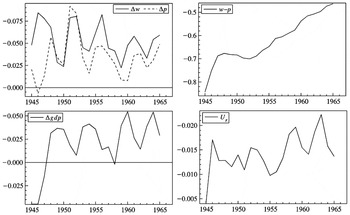
To illustrate his general findings, it seemed of interest to estimate, test, and forecast with analogous equations on the closely related annual data documented in Hendry (2001). Figure 1 records these annual time series for the period 1945–1965. As can be seen in the top-left panel, wage inflation was above 5% per annum on average and higher than price inflation, and the top-right panel confirms that real wages (w − p) rose substantially over the period. GDP growth was also high after 1947 (bottom-left panel), and correspondingly, the unemployment rate (U_r)was very low, particularly by recent standards (bottom-right panel). In this notation, lowercase letters denote logs.

Inflation, real wages, GDP growth, and unemployment in the UK.

Using the annual data shown in Figure 1, an equation of the following form can be obtained over 1946–1965 (after lagging):

In (6),

is the squared coefficient of multiple correlation,

is the residual standard deviation, coefficient standard errors are shown in parentheses, and SC is the Schwarz (1978) criterion. The diagnostic tests are of the form

, which denotes an approximate

against the alternative hypothesis

for kth-order serial correlation (

; see Godfrey, 1978), kth-order autoregressive conditional heteroskedasticity (

; see Engle, 1982), heteroskedasticity (

; see White, 1980); the RESET test (

; see Ramsey, 1969); and a chi-square test for normality (

; see Doornik and Hansen, 1994). None of these diagnostic tests is significant.

Relative to equation (17) in Sargan (1964), price inflation plays a more important role in (6) but is close to a second difference (surprise inflation). However, unemployment is insignificant, with a small positive coefficient if entered, and so it was omitted. The equilibrium solution for real wages has an annual trend (approximating productivity growth) of about 1.4% p.a., which is close to Denis's finding. The feedback coefficient is important in (6) and clearly worth retaining given the small sample. The overall fit at

is poorer than Denis reported (

, not adjusted for degrees of freedom), suggesting that intrayear information is useful, a finding that is consistent with different groups of workers agreeing on their annual wage settlements in different quarters.

Finally, expressing the equilibrium correction as

and transforming the dependent variable to real wages, leads to the more parsimonious representation

In (7), there is “short-run erosion” of real wages from price inflation, so an “inflation surprise” formulation is in fact rejected. However, the price inflation effect was probably hard to notice at the inflation rates prevalent over most of the sample against the annual growth of 1.5% from productivity gains. The disequilibrium feedback automatically offsets some of that erosion. In any case, the coefficient of Δp_t is probably not constant in the face of persistent high inflation but should decline to zero as inflation increases. Indeed, the forecast performance of (7) over the next decade of high inflation is very poor, even for one-step forecasts: testing parameter constancy to 1975 yields

(see Chow, 1960). In fact, most of this forecast failure is due to location shifts, as the equation in differences (i.e., dropping (w − p)_e,t−1) delivers

. At the time, and for many years afterward, it was not known just how susceptible “equilibrium-correction models” were to shifts in the coefficients of deterministic terms: changes to the intercept and/or trend have a pernicious effect on their performance (see, e.g., Clements and Hendry, 1999). Income policies, wage freezes, and other related governmental interventions induce such shifts, so it is unsurprising that the original specification fails to characterize the changed process. We resume this aspect of the story in Section 5.

3.11. Retrospect

It is always difficult to understand why insights are so slow in coming. The argument from long-run homogeneity by which Denis justified the equilibrium-correction term did not immediately prompt analogies or other applications, perhaps because the Colston volume was an obscure source for economists—and Denis was certainly not a propagandist. Even closer to home, Hendry and Anderson (1977) did not notice that their theoretical derivation of the equilibrium behavior of building societies was an exemplar. Indeed, it was not till after rediscovering such feedback in Davidson, Hendry, Srba, and Yeo (1978) as “the vital ‘initial disequilibrium’ effect” that those authors realized they had an example of Denis's formulation (see, e.g., Hendry, [1993] 2001). Hendry and von Ungern-Sternberg (1981) named the class “error-correction” following Phillips (1957), but its limitation to adjustment within equilibria (and not between) was not foreseen.⁴

Starting from a general specification was at best implicit in the formulation of the “transformed” model against which the autoregressive error form was to be tested. In more recent parlance, that restriction corresponded to a common factor in the lag polynomials characterizing the dynamics of the unrestricted model (see Section 4). However, Denis's “practical methodology” still included trying a variety of specifications of variables, lag lengths, indicator variables, and data transformations, probably because the sample was too small to sustain useful estimates of the nesting model and computer power was then very limited. Like many empirical investigators, Denis scrutinized the internal consistency of his results and the relationships between them, an aspect eventually formalized by encompassing.

It also remained unclear how to generalize the treatment of autoregressive errors to higher orders—the theme of the next section—perhaps because the unrestricted model was derived, rather than postulated initially. Finally, although a variety of tests for model misspecification was developed and implemented, it was not obvious whether these provided a comprehensive evaluation—or were even well behaved (see, e.g., Kiviet, 1986); Section 7 provides an update. Thus, many of the ingredients of the “LSE methodology” were in place, although a great deal of research still remained to be done.

4.1. Vector Generalizations

Sargan (1959, 1961) discussed estimating systems of dynamic equations with vector autoregressive errors. When the system was closed, there was an identification problem in extracting the error representation from the endogenous dynamics. Consider the n × 1 system in the endogenous variable y_t:

with

. The “solved” form is

Then, Π and R cannot be uniquely separated from information on Ψ₁ and Ψ₂, as they correspond to the roots—which can be arranged in many ways. Notice that an unrestricted vector autoregression (VAR) was, therefore, considered as the general model.⁵

4.2. Common Factors in Lag Polynomials

In 1975, Denis generalized the estimation of scalar dynamic equations with first-order autoregressive errors to higher order errors on equations with longer lags. Espasa (1993) describes the circumstances surrounding this development. Denis read widely, so he almost certainly knew the results in Wald (1947) and also in Anderson (1962) on the optimality of a general-to-simple approach for an ordered sequence of nested hypotheses; he cited the analysis in Anderson (1971) supporting Gets for selecting lag length.

A maximum lag length must first be carefully chosen to reflect the context (e.g., data frequency), data properties, and economic considerations, perhaps restricted by a lack of degrees of freedom. Once that has been done, consider the least restricted autoregressive model:

The Anderson procedure commenced by first testing θ_k = 0, and if that was not rejected, θ_k−1 = 0, and so on, assuming that if θ_m = 0, then θ_i = 0 for all i > m. The reduction, therefore, ceased with the first rejection.

An autoregressive-distributed lag equation with a maximum lag length of k and n “exogenous” regressors can be written as

Similar considerations could be applied for some aspects of the problem, such as lag length. Denis noted that such an approach also applied to selecting the maximal common factor. Writing (8) in an obvious notation using lag polynomials as

then an autoregressive error of order r ≤ k can be extracted if (9) can be expressed as

where all the β_i*(L) (i = 0,…,n) are now polynomials of maximum order k − r ≥ 0. Since

the terms (1 − λ_j L) are the common factors in the original lag polynomials β_i(L) (i = 0,…,n); hence the name COMFAC. Thus, an ordered sequence of hypotheses is postulated, where the existence of a common factor of order m (for m ≤ r) clearly entails the existence of all orders m − l for l > 0. Conversely, rejecting order m ≤ r entails rejecting all higher orders.

The central achievement was developing an operational algorithm to determine the largest r that could be extracted, taking account of the possibility of complex roots in the polynomials (see Sargan and Sylwestrowicz, 1976). The resulting formulation was published as Sargan (1980), although an exposition appeared in advance in Hendry and Mizon (1978).

The most obvious feature of the COMFAC viewpoint is that the initial model (9) must be the most general needed to characterize the dynamics. This is essential, both to allow extraction of the appropriate factors and so that conventional inference procedures will apply validly. Mizon (1977b) (then at the LSE) explicitly investigated model simplification routes for testing the dynamic specification of an econometric model. He considered multipath searches and the nonordered and nonsequential nature of many of the hypotheses to be tested. He stressed the need to commence from the minimally most-general specification that embedded the theory-based model. Thus, Gets was becoming the norm at LSE.