1. Introduction
The open question of regularity of the fluid dynamical equations is considered one of the most fundamental challenges of mathematics and physics (Fefferman Reference Fefferman2000). While the viscous Navier–Stokes equations have more physical relevance, the inviscid Euler equations present the greatest challenge and exhibit the most extreme behaviours. For this reason the numerical study of possible finite-time blowup is typically concerned with these inviscid equations. The three-dimensional Euler equations for an incompressible fluid of unit mass density with velocity field
 $\boldsymbol{u}(x,y,z,t)\in \mathbb{R}^{3}$
, in a time interval
 $t\,\in \,[0,T)$
, can be expressed as
 $$\begin{eqnarray}\displaystyle \frac{\partial \boldsymbol{u}}{\partial t}+\boldsymbol{u}\boldsymbol{\cdot }\boldsymbol{{\rm\nabla}}\boldsymbol{u}=-\boldsymbol{{\rm\nabla}}p,\quad \boldsymbol{{\rm\nabla}}\boldsymbol{\cdot }\boldsymbol{u}=0. & & \displaystyle\end{eqnarray}$$
Periodic boundary conditions are commonly assumed in a fundamental domain
 $[0,2{\rm\pi}]^{3}$
. Beale, Kato & Majda (Reference Beale, Kato and Majda1984) presented a blowup criterion based on the maximum vorticity (infinity norm), thus providing an important reference for diagnosing singularities numerically (BKM theorem). The literature surrounding the numerical assessment of finite-time blowup in 3D Euler flows is extensive and will not be reviewed in detail here (see Bardos & Titi (Reference Bardos and Titi2007) and Gibbon (Reference Gibbon2008), and for references pertinent to the current work see the introduction in Mulungye, Lucas & Bustamante (Reference Mulungye, Lucas and Bustamante2015)); suffice to say that a fundamental difficulty of this important problem is the lack of analytic solutions or any a priori knowledge of asymptotic behaviour. A secondary obstacle is that the spatial collapse associated with intense vortex stretching results in numerical solutions becoming unresolved beyond a certain time (e.g. loss of spectral convergence). It is therefore these authors’ view that it is imperative to devise a framework with non-trivial blowup dynamics and where analytic solutions are known in order to validate and compare various numerical methods, for the purposes of accurately solving the system and diagnosing blowup. In this regard we reinvestigate the infinite-energy, stagnation-point-type solutions of the 3D Euler equations (Gibbon, Fokas & Doering Reference Gibbon, Fokas and Doering1999), which exhibit finite-time blowup that can be assessed analytically (Constantin Reference Constantin2000), now employing a novel method that maps, bijectively and nonlinearly, the time and fields to a globally regular system (Bustamante Reference Bustamante2011). Crucially, the singularity time
 $t=T^{\ast }$
maps to
 ${\it\tau}=\infty$
in the new time variable. This helps us uncover a curious late-time behaviour of the Fourier spectrum: the solution remains well converged spectrally at times
 $t$
close to singularity time
 $T^{\ast }$
well within floating-point precision:
 $T^{\ast }-t\ll 10^{-16}$
. We find that the mapped variables maintain acceptable levels of error in the main blowup quantities such as the
 $L^{\infty }$
and
 $L^{2}$
norms of the vortex stretching rate at this extreme closeness to
 $T^{\ast }.$
We begin by formulating both the original and mapped equations and reviewing and updating the analytic and asymptotic results for blowup. We then present a thorough investigation of the Fourier spectra of the solution, followed by error analysis of our numerics and an assessment of singularity time and proximity to it.
2. Formulation
We consider a class of exact solutions of the 3D Euler equations presented by Gibbon et al. (Reference Gibbon, Fokas and Doering1999). Writing
 $\boldsymbol{u}(x,y,z,t)=(u_{x}(x,y,t),u_{y}(x,y,t),z\,{\it\gamma}(x,y,t))$
, we obtain
 $$\begin{eqnarray}\displaystyle & \displaystyle \frac{\partial {\it\gamma}}{\partial t}+\boldsymbol{u}_{\mathit{h}}\boldsymbol{\cdot }\boldsymbol{{\rm\nabla}}_{\mathit{h}}{\it\gamma}=2\langle {\it\gamma}^{2}\rangle -{\it\gamma}^{2}, & \displaystyle\end{eqnarray}$$
 $$\begin{eqnarray}\displaystyle & \displaystyle \frac{\partial {\it\omega}}{\partial t}+\boldsymbol{u}_{\mathit{h}}\boldsymbol{\cdot }\boldsymbol{{\rm\nabla}}_{\mathit{h}}{\it\omega}={\it\gamma}\,{\it\omega}, & \displaystyle\end{eqnarray}$$
 $\boldsymbol{u}_{\mathit{h}}(x,y,t)\equiv (u_{x}(x,y,t),u_{y}(x,y,t))$
denotes the ‘horizontal’ component of the velocity field at the symmetry plane (
 $z=0$
),
 $\boldsymbol{{\rm\nabla}}_{\mathit{h}}=(\partial _{x},\partial _{y})$
denotes the ‘horizontal’ gradient operator,
 ${\it\omega}(x,y,t)=\partial _{x}u_{y}-\partial _{y}u_{x}$
is the vorticity,
 ${\it\gamma}$
is the stretching rate of vorticity, which using the incompressibility condition in (1.1) can be defined as
 ${\it\gamma}(x,y,t)=-\boldsymbol{{\rm\nabla}}_{\mathit{h}}\boldsymbol{\cdot }\boldsymbol{u}_{\mathit{h}}(x,y,t)$
, and
 $\langle f(\cdot ,t)\rangle \equiv (1/4{\rm\pi}^{2})\int _{0}^{2{\rm\pi}}\int _{0}^{2{\rm\pi}}f(x,y,t)\,\text{d}x\,\text{d}y$
denotes the spatial average over the periodic 2D domain.
Constantin (Reference Constantin2000) solved for
 ${\it\gamma}$
along characteristics (and for vorticity
 ${\it\omega}$
, which can be found a posteriori), proving that the stretching rate
 ${\it\gamma}$
would blow up in a finite time, with explicit formulae for the singularity time that confirmed the accuracy of the numerical blowup predictions by Ohkitani & Gibbon (Reference Ohkitani and Gibbon2000). A BKM (Beale et al.
Reference Beale, Kato and Majda1984) type of theorem was established by Gibbon & Ohkitani (Reference Gibbon and Ohkitani2001) where the blowup time
 $T^{\ast }$
is defined as the smallest time at which
 $\int _{0}^{T^{\ast }}\Vert {\it\gamma}(\cdot ,t^{\prime })\Vert _{\infty }~\text{d}t^{\prime }=\infty ,$
where
 $\Vert {\it\gamma}(\cdot ,t)\Vert _{\infty }$
is the supremum norm of the vorticity stretching rate.
Bustamante (Reference Bustamante2011) and later Mulungye et al. (Reference Mulungye, Lucas and Bustamante2015) introduced the following ‘mapped’ fields and ‘mapped’ time:
 $$\begin{eqnarray}\left.\begin{array}{@{}c@{}}\displaystyle {\it\gamma}_{\mathit{map}}(x,y,{\it\tau})=\frac{{\it\gamma}(x,y,t)}{\Vert {\it\gamma}(\cdot ,t)\Vert _{\infty }},\quad {\it\tau}(t)=\int _{0}^{t}\Vert {\it\gamma}(\cdot ,t^{\prime })\Vert _{\infty }~\text{d}t^{\prime },\\ \displaystyle {\it\omega}_{\mathit{map}}(x,y,{\it\tau})=\frac{{\it\omega}(x,y,t)}{\Vert {\it\gamma}(\cdot ,t)\Vert _{\infty }},\quad \boldsymbol{u}_{\mathit{map}}(x,y,{\it\tau})=\frac{\boldsymbol{u}_{\mathit{h}}(x,y,t)}{\Vert {\it\gamma}(\cdot ,t)\Vert _{\infty }}.\end{array}\right\}\end{eqnarray}$$
This transformation is bijective for
 $t<T^{\ast }$
. The mapped fields satisfy the following system of partial differential equations:
 $$\begin{eqnarray}\displaystyle & \displaystyle \frac{\partial {\it\gamma}_{\mathit{map}}}{\partial {\it\tau}}+\boldsymbol{u}_{\mathit{map}}\boldsymbol{\cdot }\boldsymbol{{\rm\nabla}}{\it\gamma}_{\mathit{map}}=2\langle {\it\gamma}_{\mathit{map}}^{2}\rangle -{\it\gamma}_{\mathit{map}}^{2}+{\it\sigma}_{\infty }{\it\gamma}_{\mathit{map}}\{1-2\langle {\it\gamma}_{\mathit{map}}^{2}\rangle \} & \displaystyle\end{eqnarray}$$
 $$\begin{eqnarray}\displaystyle & \displaystyle \frac{\partial {\it\omega}_{\mathit{map}}}{\partial {\it\tau}}+\boldsymbol{u}_{\mathit{map}}\boldsymbol{\cdot }\boldsymbol{{\rm\nabla}}{\it\omega}_{\mathit{map}}={\it\gamma}_{\mathit{map}}\,{\it\omega}_{\mathit{map}}+{\it\sigma}_{\infty }{\it\omega}_{\mathit{map}}\{1-2\langle {\it\gamma}_{\mathit{map}}^{2}\rangle \}, & \displaystyle\end{eqnarray}$$
 ${\it\sigma}_{\infty }\equiv \text{sgn}\,{\it\gamma}(\boldsymbol{X}_{{\it\gamma}}(t),t)$
is the sign of
 ${\it\gamma}$
at the position
 $\boldsymbol{X}_{{\it\gamma}}(t)$
of maximum
 $|{\it\gamma}(\boldsymbol{x},t)|$
. The initial conditions used in this study are
 ${\it\gamma}_{0}(x,y)={\it\omega}_{0}(x,y)=\sin (x)\sin (y)$
.
2.1. Analytical solution of the stagnation-point-type 3D Euler flows
Solutions of (2.1)–(2.2) are exact solutions of
 $3$
D Euler equations (albeit with infinite energy), as derived originally by Gibbon et al. (Reference Gibbon, Fokas and Doering1999). Ohkitani & Gibbon (Reference Ohkitani and Gibbon2000) performed a numerical study at resolution
 $256^{2},$
supported with simulations at resolution
 $1024^{2},$
which provided evidence of a finite-time singularity at
 $t\approx 1.4$
. Higher resolution was not needed because spectral convergence was observed during most of the simulation time.
Constantin (Reference Constantin2000) introduced a method for finding the blowup quantities (e.g.
 $\Vert {\it\gamma}(\cdot ,t)\Vert _{\infty },\,\langle {\it\gamma}^{2}\rangle$
) analytically and established that there is a finite-time singularity. While it is possible to obtain the asymptotic behaviour of the blowup quantities using the method of Constantin (Reference Constantin2000), we will discuss this in the context of our method (Mulungye et al.
Reference Mulungye, Lucas and Bustamante2015) for the purposes of simplicity of presentation. There, the auxiliary function
 $S(t)$
that provides the solution for all fields along characteristics (see Mulungye et al. (Reference Mulungye, Lucas and Bustamante2015) for more details) satisfies an ordinary differential equation which, for our choice of initial conditions, reads
 $$\begin{eqnarray}{\dot{S}}=\frac{{\rm\pi}^{2}}{4\,[K(S^{2})]^{2}},\quad S(0)=0,\end{eqnarray}$$
where
 $K({\it\mu}^{2})$
is the complete elliptic function of the first kind. Thus
 $S$
can be interpreted in this case as the modulus of the elliptic function. The singularity occurs when
 $S=S^{\ast }$
, where
 $S^{\ast }\equiv -1/\inf {\it\gamma}_{0}=1$
. Thus,
 $S(t)$
goes from
 $0$
at
 $t=0$
to
 $1$
at
 $t=T^{\ast }$
, where
 $T^{\ast }$
is the singularity time defined as
 $$\begin{eqnarray}\displaystyle T^{\ast }=\frac{4}{{\rm\pi}^{2}}\int _{0}^{1}[K(S^{2})]^{2}\,\text{d}S\approx 1.418002734923858875062234. & & \displaystyle\end{eqnarray}$$
Ohkitani & Gibbon (Reference Ohkitani and Gibbon2000) estimated
 $T^{\ast }\approx 1.417$
, which appears to be a good estimate, but, as we will show, is not close enough to capture the true late-time dynamics.
The singularity is dominated by the infimum of
 ${\it\gamma}(\boldsymbol{x},t)$
, and for these initial conditions we can identify
 $\Vert {\it\gamma}\Vert _{\infty }=-\inf {\it\gamma},$
so
 ${\it\sigma}_{\infty }=-1$
will be used throughout. It is also possible to obtain some exact formulae for
 $\Vert {\it\gamma}(\cdot ,t)\Vert _{\infty }$
and
 ${\it\tau}(t)$
in implicit form through
 $S(t)$
:
 $$\begin{eqnarray}{\it\tau}(t)=-\ln \left(\frac{2}{{\rm\pi}}(1-S)K(S^{2})\right),\end{eqnarray}$$
 $$\begin{eqnarray}-\inf _{\boldsymbol{x}\in \mathbb{T}^{2}}{\it\gamma}(\boldsymbol{x},t)=\Vert {\it\gamma}(\cdot ,t)\Vert _{\infty }=\frac{{\rm\pi}^{2}[(S+1)K(S^{2})-E(S^{2})]}{4S(1-S^{2})K(S^{2})^{3}},\end{eqnarray}$$
 $$\begin{eqnarray}\left\langle {\it\gamma}^{2}\right\rangle =\frac{{\rm\pi}^{4}[K(S^{2})-E(S^{2})]\,[2E(S^{2})-(1-S^{2})K(S^{2})]}{32S^{2}(1-S^{2})^{2}K(S^{2})^{6}}.\end{eqnarray}$$
Notice that it is possible to find
 $S(t({\it\tau}))$
and
 $\Vert {\it\gamma}(\cdot ,t({\it\tau}))\Vert _{\infty }$
as functions of
 ${\it\tau}$
via first inverting (2.8) to obtain
 $S(t({\it\tau})),$
and then using this on (2.9) to obtain
 $\Vert {\it\gamma}(\cdot ,t({\it\tau}))\Vert _{\infty }$
. For the error analysis of § 3.2 we will use a numerical solution of the ordinary differential equation (2.6) for
 $S(t)$
(in principle feasible to any desired accuracy), because a closed form is not available. For this reason we term this solution quasi-analytic. At values of
 ${\it\tau}$
greater than about
 $33,$
this requires the use of arbitrary-precision arithmetic, provided by commercial packages such as Mathematica, as
 $1-10^{-16}<S(t)<1$
, i.e. double floating-point precision is lost.
Alternatively, at late times the solution
 $S(t)$
can be constructed using asymptotic formulae accurate to double precision. Defining
 $Z\equiv -\!\ln [(1-S)/8]$
, the following formulae are valid asymptotically as
 $S\rightarrow 1^{-}$
(i.e. as
 ${\it\tau}\rightarrow \infty$
):
 $$\begin{eqnarray}\displaystyle \hspace{-18.0pt}\left.\begin{array}{@{}c@{}}\displaystyle {\it\tau}\approx Z-\ln \left(\frac{8Z}{{\rm\pi}}\right),\quad Z\approx -W_{-1}\left(-\frac{1}{8}{\rm\pi}\text{e}^{-{\it\tau}}\right),\quad T^{\ast }-t\approx \frac{8\text{e}^{-Z}}{{\rm\pi}^{2}}(Z^{2}+2Z+2),\\ \displaystyle \Vert {\it\gamma}(\cdot ,t)\Vert _{\infty }\approx \frac{{\rm\pi}^{2}\text{e}^{Z}}{8}\left(\frac{Z-1}{Z^{3}}\right),\quad \left\langle {\it\gamma}^{2}\right\rangle \approx \frac{{\rm\pi}^{4}\text{e}^{2Z}}{128}\left(\frac{Z-2}{Z^{6}}\right),\end{array}\right\} & & \displaystyle \nonumber\\ \displaystyle & & \displaystyle\end{eqnarray}$$
 $W_{-1}$
is a branch of the Lambert function. We can combine the above to obtain explicit asymptotic expressions for
 $T^{\ast }-t$
and
 $\Vert {\it\gamma}(\cdot ,t)\Vert _{\infty }$
in terms of the mapped time
 ${\it\tau}$
. These asymptotic formulae are very useful in practice. At
 ${\it\tau}=5$
the above asymptotic formula for
 $t({\it\tau})$
has a relative error of about
 $10^{-9}$
and for
 $\Vert {\it\gamma}(\cdot ,t)\Vert _{\infty },$
a relative error of
 $10^{-7}$
. By
 ${\it\tau}>20$
the asymptotic formulae above are accurate to double precision (
 $10^{-16}$
), giving a much simpler route to computing the blowup quantities. Thus, for small
 ${\it\tau}$
we will use the quasi-analytic solution and for large
 ${\it\tau}$
we will use the asymptotic solution, in order to assess the errors between direct numerical simulations and analytical formulae for the blowup quantities in § 3.2.
3. Numerical solution of original and mapped systems
We solve the evolution equations for both systems numerically using a standard pseudospectral method implemented on GPUs using CUDA (Mulungye et al.
Reference Mulungye, Lucas and Bustamante2015). Dealiasing is carried out using Hou’s exponential filter
 $\exp (-36(2k/N)^{36})$
(for a given spatial resolution
 $N$
) (Hou & Li Reference Hou and Li2006), and a fourth-order Runge–Kutta scheme solves in time. Adaptive time stepping (
 $\text{d}t=\text{d}{\it\tau}/\Vert {\it\gamma}(\cdot ,t)\Vert _{\infty }$
) is used for the original equations and uniform steps of
 $\text{d}{\it\tau}$
are used in the mapped system with the resulting distribution of temporal data roughly equivalent.
3.1. Spectra and analyticity strip
To investigate the spatial collapse associated with the blowup, we consider a detailed analysis of the one-dimensional spectra of stretching rate constructed from circular shells,
 $$\begin{eqnarray}E(k,t)=\mathop{\sum }_{k-(1/2)<|\boldsymbol{k}|<k+(1/2)}|\hat{{\it\gamma}}(\boldsymbol{k},t)|^{2}.\end{eqnarray}$$
Our first observation of the evolution of the spectrum is that there are two time scales in evidence. An initial burst can be observed with a flux towards intermediate
 $k$
that is redistributed across the modes. Provided
 $N>256$
this initial phase remains well resolved and lasts only until
 ${\it\tau}\approx 25$
. Thereafter there is a slow cascade from small
 $k$
. In fact in original variables the initial phase is until
 $T^{\ast }-t\approx 10^{-10}$
. As will be shown, this is too early to establish certain asymptotic trends.
We also found that, due to the lack of direct energy cascade to large
 $k$
, an accumulation of round-off error propagates up-scale. The result is a small quantity of spurious energy between the large scales and the truncation wavenumber. The amount of this spurious energy is dependent on resolution, leading to an ill-converged spectrum. We remedy this by applying a small amount of hyperviscosity on the large wavenumbers, namely adding the term
 ${\it\nu}(-1)^{2h+1}|\boldsymbol{k}|^{2h}\hat{{\it\gamma}}$
for
 $|\boldsymbol{k}|>200$
, with
 $h=2$
, to the right-hand side of the Fourier transform of (2.4) and an equivalent term for
 $\hat{{\it\omega}}$
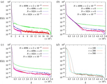
in (2.5). Numerically a Crank–Nicolson scheme was used on this term for stability. Figure 1 shows the profile of the spectra at
 ${\it\tau}=5,$
 $10$
and
 $25$
for
 $N=1024$
and
 $4096,$
each with
 ${\it\nu}=10^{-9}$
and
 ${\it\nu}=0$
. This demonstrates that the hyperviscosity gives a well converged spectrum while leaving the large-scale modes unaffected. The error in the bulk quantity
 $\langle {\it\gamma}_{\mathit{map}}^{2}\rangle$
is unchanged (figure not shown), but applying hyperviscosity to all modes leads to a significant increase in error.
Interestingly the late-time profile does not have the typical shape we might expect (Bustamante & Brachet Reference Bustamante and Brachet2012; Mulungye et al. Reference Mulungye, Lucas and Bustamante2015) or that which has been assumed previously in this system (Ohkitani & Gibbon Reference Ohkitani and Gibbon2000), namely
 $$\begin{eqnarray}E(k,t)\lessapprox C(t)k^{-n(t)}\text{e}^{-2{\it\delta}_{1}(t)k}.\end{eqnarray}$$
In fact, as can be seen in figure 1 (bottom right at late times), the profile assumes a more Gaussian shape,
 $$\begin{eqnarray}E(k,t)\lessapprox C(t)k^{-n(t)}\text{e}^{-({\it\delta}_{2}(t)k)^{2}}.\end{eqnarray}$$
This late-time spatial form has been missed in previous work (Ohkitani & Gibbon Reference Ohkitani and Gibbon2000) on this system because it arises only after the initial burst, which does have the
 $\text{e}^{-2{\it\delta}k}$
shape, and persists to sufficiently close to
 $T^{\ast }$
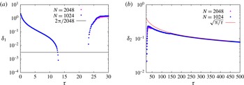
to render it next to inaccessible without the mapped variables. To ensure the convergence of the initial burst phase we first perform a least-squares fitting procedure to the spectrum with ansatz (3.2). Figure 2 shows the fitted
 ${\it\delta}_{1}$
for the early burst phase. The plot shows two resolutions (
 $N=1024$
and 2048), which are essentially indistinguishable. From figure 1 the exponential part of the profile of
 $E(k,t)$
is preceded (in
 $k$
) by the Gaussian shape. The down-scale flux associated with the slackening of the exponential part (
 ${\it\delta}_{1}$
decreasing) establishes the Gaussian profile in its wake. The result is that, while the trend in
 ${\it\delta}_{1}$
suggests an exponential decay in
 ${\it\tau}$
(at early times), in reality the ansatz (3.2) ceases to be a valid analyticity measure due to the addition of a large-scale Gaussian spectrum. The cross-over regime is indicated by negative values of
 ${\it\delta}_{1}$
for
 $13\lesssim {\it\tau}\lesssim 23$
.
To analyse the true late-time behaviour (
 ${\it\tau}>25$
) we fit with ansatz (3.3). Figure 2 shows the behaviour of
 ${\it\delta}_{2}$
as a function of
 ${\it\tau}$
. Strikingly, the decay is now very slow (see (3.7)).
Snapshots of spectra for
 ${\it\tau}=5$
, 10 and 25 ((a), (b) and (c) respectively), on a lin–log scale. Panels (a–c) show two resolutions (
 $N=1024$
and 4096), with and without hyperviscosity, demonstrating the need to control floating-point round-off error at small scales. Panel (a) shows the full spectrum, including dealiased filtered modes to show the small-scale error. Thereafter, panels (b,c) show only the first 500 modes to make clear the initial burst and the onset of the slow Gaussian spectrum ((a)
 $t=1.396$
;
 $T^{\ast }-t\approx 0.022$
; (b)
 $t=1.41778$
;
 $T^{\ast }-t\approx 0.00022$
; (c)
 $t=1.418002734785$
;
 $T^{\ast }-t=1.4\times 10^{-10}$
). Panel (d) shows only the
 $N=1024$
case with hyperviscosity
 $({\it\nu}=10^{-10})$
, now with curves at
 ${\it\tau}=100$
, 200 and 500 showing the slow broadening of the spectrum at late times.

Time evolution of the analyticity distance
 ${\it\delta}({\it\tau})$
of the Fourier spectrum of
 ${\it\gamma}^{2}$
. (a) Profile at early times based on (3.2), showing the initial burst. (b) Late-time profile based on (3.3) showing the slow Gaussian cascade along with the estimate
 ${\it\delta}\approx \sqrt{{\rm\pi}/{\it\tau}}$
, which saturates inequality (3.7).

Using a classical method, it is possible to obtain a rigorous upper bound for the supremum norm of stretching rate in terms of the spectrum:
 $$\begin{eqnarray}\displaystyle & \displaystyle \Vert {\it\gamma}(\cdot ,t)\Vert _{\infty }\leqslant \mathop{\sum }_{k=1}^{\infty }\sqrt{p_{k}}\sqrt{E(k,t)}, & \displaystyle \nonumber\\ \displaystyle & \displaystyle p_{k}\equiv \#\{\boldsymbol{k}\in \mathbb{Z}_{\mathit{odd}}^{2}\cup \mathbb{Z}_{\mathit{even}}^{2}:k-1/2<|\boldsymbol{k}|<k+1/2\}\approx {\rm\pi}\,k,\quad k\rightarrow \infty . & \displaystyle\end{eqnarray}$$
The special condition on odd–odd or even–even modes is due to the discrete symmetry of our initial condition.
Replacing the fit (3.3) into (3.4) leads to a bound involving an infinite sum over
 $k$
with an ultraviolet divergence in the limit of small
 ${\it\delta}(t)$
. We can approximate this as follows (Bustamante & Brachet Reference Bustamante and Brachet2012):
 $$\begin{eqnarray}\Vert {\it\gamma}(\cdot ,t)\Vert _{\infty }\leqslant \frac{1}{2}\sqrt{{\rm\pi}C(t)}\,{\it\Gamma}\left(1-\frac{n(t)+1}{4}\right)\,\left[\frac{1}{2}{\it\delta}(t)^{2}\right]^{(n(t)+1)/4-1},\end{eqnarray}$$
where
 ${\it\Gamma}$
is the gamma (factorial) function. A further improvement is obtained by noticing the behaviour of
 $n(t)$
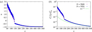
at late times from figure 3, where it is clear that
 $n(t)\rightarrow -1$
. Therefore we obtain, in this limit,
 $$\begin{eqnarray}\Vert {\it\gamma}(\cdot ,t)\Vert _{\infty }\leqslant \sqrt{{\rm\pi}C(t)}\,{\it\delta}(t)^{-2}.\end{eqnarray}$$
This inequality alone cannot be used to estimate the behaviour of
 ${\it\delta}(t),$
since the independent factor
 $C(t)$
is involved as well, so an extra equation is needed. This extra equation is provided by combining the asymptotic formulae (2.11):
 $\langle {\it\gamma}(\cdot ,t)^{2}\rangle \approx \Vert {\it\gamma}(\cdot ,t)\Vert _{\infty }^{2}/2{\it\tau}$
. The left-hand side of this equation can be written in terms of the energy spectrum, so if we follow similar steps as in the derivation of inequality (3.6) we obtain
 $\langle {\it\gamma}(\cdot ,t)^{2}\rangle \approx (C(t)/2){\it\delta}(t)^{-2},$
and therefore we get
 $C(t)\approx \Vert {\it\gamma}(\cdot ,t)\Vert _{\infty }^{2}\,{\it\delta}(t)^{2}/{\it\tau}$
. Using this we can go back to inequality (3.6) and show that it is equivalent to
 $$\begin{eqnarray}{\it\delta}(t)\leqslant \sqrt{\frac{{\rm\pi}}{{\it\tau}}}.\end{eqnarray}$$
This inequality is in fact saturated, as confirmed by our numerical simulation (figure 2). In terms of original time variable we get
 ${\it\delta}(t)\leqslant \sqrt{{\rm\pi}/(-W_{-1}(-{\rm\pi}(T^{\ast }-t)))}\approx \sqrt{{\rm\pi}/(-\ln ({\rm\pi}(T^{\ast }-t)))},$
which illustrates that the loss of regularity is very slow in the original time variable. In fact if one were to consider the reliability time with the saturated spectrum one would find that
 ${\it\tau}_{rel}\approx N^{2}/4{\rm\pi}$
, so that for
 $N=512,$
 ${\it\tau}_{rel}\approx 2\times 10^{4}$
or
 $T^{\ast }-t\approx 10^{-9000}$
.
Time evolution of the exponent,
 $n(t({\it\tau}))$
, and constant factor,
 $C(t({\it\tau}))$
(normalised to coincide with the mapped variables), of the fit ansatz equation (3.3) of the Fourier spectrum of
 ${\it\gamma}^{2}$
. Alongside
 $C(t({\it\tau}))$
is the saturated estimate
 ${\rm\pi}{\it\tau}^{-2}$
from inequalities (3.4) and (3.7).

3.2. Errors
Here we assess the errors between direct numerical simulations (DNS) and analytical formulae for the blowup quantities, in order to establish superiority of the accuracy of the mapped system over that of the original system. Using the definition in Perlin & Bustamante (Reference Perlin and Bustamante2015), the ‘normalised’
 $L^{2}$
norm of the error (not relative error) is given by
 $Q(f,g)=\Vert f-g\Vert _{2}/(\Vert f\Vert _{2}+\Vert g\Vert _{2}).$
We consider the errors
 $Q_{{\it\gamma}}=Q(\Vert {\it\gamma}_{\mathit{num}}(\cdot ,t)\Vert _{\infty },\Vert {\it\gamma}_{\mathit{ana}}(\cdot ,t)\Vert _{\infty })$
and
 $Q_{\langle {\it\gamma}^{2}\rangle }=Q(\langle {\it\gamma}_{\mathit{num}}^{2}\rangle ,\langle {\it\gamma}_{\mathit{ana}}^{2}\rangle )$
, with corresponding mapped equivalents, where the subscripts ‘num’ and ‘ana’ stand for ‘numerical’ (i.e. from DNS) and ‘analytic’. As described in § 2.1 the ‘analytic’ solution is the quasi-analytic form at early
 ${\it\tau}$
, (2.8)–(2.10), and the asymptotic formulae (2.11) at late
 ${\it\tau}$
.
The numerical solution of the mapped system does not provide direct access to the original variable
 $\Vert {\it\gamma}(\cdot ,t)\Vert _{\infty }$
so the following expression is required (Mulungye et al.
Reference Mulungye, Lucas and Bustamante2015):
 $$\begin{eqnarray}\Vert {\it\gamma}(\cdot ,t({\it\tau}))\Vert _{\infty }=\Vert {\it\gamma}_{0}\Vert _{\infty }\exp \left[{\it\tau}-2\int _{0}^{{\it\tau}}\langle {\it\gamma}_{\mathit{map}}^{2}\rangle \,\text{d}{\it\tau}^{\prime }\right]\,,\end{eqnarray}$$
where
 $\int _{0}^{{\it\tau}}\langle {\it\gamma}_{\mathit{map}}^{2}\rangle \,\text{d}{\it\tau}^{\prime }$
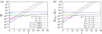
is computed using Simpson’s rule. We compare both this mapped estimate and the direct supremum norm from the original system against the analytical solution of (2.9). Care is taken in solving (2.6) so that the time steps from the original system are used to solve on intervals that coincide with the data points, and arbitrary precision of the required level is used. As shown in the previous section the solution remains well resolved spatially, even at relatively modest resolutions, therefore we omit the error study of spatial convergence here. We do, however, show convergence with respect to time step
 $\text{d}{\it\tau}$
in figure 4 at resolution
 $N=1024$
. Overall we observe an exponential growth (in
 ${\it\tau}$
) of
 $Q_{{\it\gamma}}$
from the original system, compared to an almost uniform error (
 ${\sim}10^{-10}$
) from the mapped version at converged
 $\text{d}{\it\tau}$
. Interestingly convergence occurs in the mapped system at a smaller level of
 $\text{d}{\it\tau}$
.
In contrast to the earlier result in Mulungye et al. (Reference Mulungye, Lucas and Bustamante2015), we find that both
 $Q_{{\it\gamma}}$
and
 $Q_{\langle {\it\gamma}_{\mathit{map}}^{2}\rangle }$
behave similarly; recall that
 $\langle {\it\gamma}_{\mathit{map}}^{2}\rangle$
is the primary variable for the assessment of the local quantity
 $\Vert {\it\gamma}(\cdot ,t)\Vert _{\infty }$
in the mapped system (3.8). This implies that in this case (where
 $\langle {\it\gamma}^{2}\rangle$
is not an invariant),
 $Q_{{\it\gamma}}$
is simply slaved to
 $Q_{\langle {\it\gamma}_{\mathit{map}}^{2}\rangle }$
. Mulungye et al. (Reference Mulungye, Lucas and Bustamante2015) contains a detailed discussion on error sources in the mapped and original variables, and highlights some subtleties surrounding the behaviour of
 $\langle {\it\gamma}^{2}\rangle$
. Here the situation is somewhat more straightforward: the original system contains unbounded error growth due to a fundamental loss of precision in the independent variable. This is explained by the earlier convergence and the ‘saturation’ of error near the double-precision limit (
 ${\it\tau}\approx 37$
).
Time evolution of the error measures
 $Q_{{\it\gamma}}$
(a),
 $Q_{\langle {\it\gamma}_{\mathit{map}}^{2}\rangle }$
and
 $Q_{\langle {\it\gamma}^{2}\rangle }$
(b), showing the convergence with time step
 $\text{d}{\it\tau}$
.

3.3. Assessing blowup time
 $T^{\ast }$
and proximity to it,
$T^{\ast }-t$


Previous methods for assessing the value of
 $T^{\ast },$
e.g. fitting the behaviour of
 $\Vert {\it\gamma}(\cdot ,t)\Vert _{\infty }$
to a power law
 $(T^{\ast }-t)^{{\it\alpha}},$
are based on the assumption that the solution incurs significant errors at intermediate time and
 $T^{\ast }$
requires careful extrapolation. Here the solution remains well resolved until late times and we find that if we use the original system with the adaptive time step given above,
 $t$
converges to
 $T^{\ast }$
to within
 ${\sim}10^{-14}$
. This accuracy is surprising given that it arises from a simple sum
 $t_{n}=\sum _{i=0}^{n}\,\text{d}{\it\tau}/\Vert {\it\gamma}(\cdot ,t_{i})\Vert _{\infty },$
and it cannot be improved by fitting or even by arbitrary-precision arithmetic to sum values of
 $\text{d}t$
that are below the machine precision threshold. Understanding this accuracy is aided by attempting the comparable exercise for the mapped system. Here the recovery of
 $t$
is given by
 $t({\it\tau})=\int _{0}^{{\it\tau}}1/(\Vert {\it\gamma}(\cdot ,t({\it\tau}^{\prime }))\Vert _{\infty })\,\text{d}{\it\tau}^{\prime }\,,$
where
 $\Vert {\it\gamma}(\cdot ,t({\it\tau}^{\prime }))\Vert _{\infty }$
is obtained from formula (3.8). This integral should converge to
 $T^{\ast }$
as
 ${\it\tau}\rightarrow \infty$
. Computing it numerically results in a saturation of error
 ${\sim}10^{-9}$
(slaved to the error in
 $\Vert {\it\gamma}(\cdot ,t({\it\tau}))\Vert _{\infty }$
) when
 $\text{d}{\it\tau}=10^{-4}$
for sufficiently large
 ${\it\tau}$
. This almost leads to a paradox: why should a quantity with lower late-time error produce a poorer estimate for
 $T^{\ast }$
when the procedure for the estimate is qualitatively the same? The reason is that it is the early errors that pollute the estimate for
 $t({\it\tau})$
because these are larger in the mapped system and occur at a point where they will contribute more significantly to the final integral (
 $\text{d}{\it\tau}/\Vert {\it\gamma}(\cdot ,t)\Vert _{\infty }$
is largest).
However, one should proceed with caution when dismissing the ability of the mapped system to assess its original temporal position: error in the assessment of
 $T^{\ast }$
is not to be confused with error in the proximity to
 $T^{\ast }$
. Although the original system can integrate to within
 $10^{-14}$
of
 $T^{\ast }$
, it is impossible to assess any behaviour beyond this point: convergence of
 $t$
to this value means this is a solid barrier for the method. This is not the case for the mapped system: through
 $t({\it\tau})$
we can produce an estimate for
 $T^{\ast }-t$
as a function of
 ${\it\tau}$
by considering the following ‘proximity’ integral:
 $$\begin{eqnarray}T^{\ast }-t\approx P({\it\tau})=\int _{{\it\tau}}^{\infty }\frac{1}{\Vert {\it\gamma}(\cdot ,t({\it\tau}^{\prime }))\Vert _{\infty }}\,\text{d}{\it\tau}^{\prime }.\end{eqnarray}$$
Recalling that
 $\Vert {\it\gamma}(\cdot ,t)\Vert _{\infty }$
is recovered from
 $\langle {\it\gamma}_{\mathit{map}}^{2}\rangle$
in the mapped system via formula (3.8), we fit the behaviour of this global measure in the preceding
 $({\it\tau}-10)$
window via the ansatz
 $\langle {\it\gamma}_{\mathit{map}}^{2}\rangle \sim {\it\kappa}-m/{\it\tau}$
. Inserting this into what is now the double integral for
 $T^{\ast }-t$
, we obtain
 $$\begin{eqnarray}P({\it\tau})\approx \frac{\text{e}^{(1-2{\it\kappa}){\it\tau}}{\it\tau}^{2m}(1-2{\it\kappa})^{2m}}{\Vert {\it\gamma}(\cdot ,t({\it\tau}))\Vert _{\infty }}{\it\Gamma}(1-2m,(1-2{\it\kappa}){\it\tau}),\end{eqnarray}$$
where
 ${\it\Gamma}$
is the incomplete gamma function. This provides a running estimate for
 $T^{\ast }-t$
that we can validate against the asymptotic formula, (2.11). Figure 5 shows the relative error in
 $P({\it\tau})$
as a function of
 $T^{\ast }-t$
in order to demonstrate how the error depends on the absolute proximity to
 $T^{\ast }$
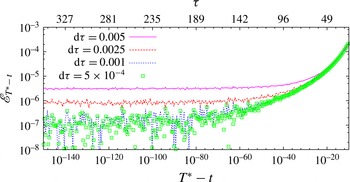
. We find relative errors of the order of
 $10^{-7}$
persisting far beyond the machine precision limit, and converging at larger
 $\text{d}{\it\tau}$
than
 $Q_{{\it\gamma}},$
presumably due to the accuracy of the fitting procedure.
Relative error of proximity
 $P({\it\tau})$
compared to the asymptotic formula (2.11) plotted against
 $T^{\ast }-t$
(bottom axis) and
 ${\it\tau}$
(top axis). Curves show convergence in
 $\text{d}{\it\tau}$
and an error
 ${\sim}10^{-7}$
persistent to exceptionally small values of
 $T^{\ast }-t$
.

4. Conclusion and discussion
In this paper we have shown that only by mapping the singular system (2.1)–(2.2) to a regular one (2.4)–(2.5) can certain unconventional late-time behaviours be observed and asymptotic trends be established. The first unusual feature shown is the slow spatial collapse and unusual (Gaussian) Fourier spectrum very near singularity time. This means that the solution will remain well spectrally converged until extraordinarily close to singularity time for even modest resolutions. In turn this implies a fundamental constraint on the original system: in the original variables one can only hope to approach
 $T^{\ast }$
to the precision of the floating-point arithmetic being used, usually double precision,
 ${\approx}10^{-16}$
. Because of this lack of digits in the independent temporal variable, assessing any quantities from the original system is a hazardous undertaking as errors grow exponentially. In other words, not only does the proximity to
 $T^{\ast }$
present a floating-point barrier, it also harms the accurate assessment of the late-time behaviour of the system before the barrier is reached. On the other hand, the mapped system has no floating-point arithmetic barrier as the singularity time is now at infinity and we observe uniform errors until
 $T^{\ast }-t$
is exceptionally small (
 $10^{-140}$
in the figures shown).
Another floating-point barrier also becomes apparent, namely that
 $\Vert {\it\gamma}\Vert _{\infty }$
will eventually overflow, i.e. exceed
 ${\sim}10^{308}$
at
 ${\it\tau}\approx 715$
. Luckily the mapping allows us to postpone this barrier further by simply computing
 $\log \Vert {\it\gamma}\Vert _{\infty }$
(i.e. outputting the exponent of the right-hand side of (3.8)) and use an arbitrary-precision exponential in post-processing if required.
One may now ask: what relevance do these results have to the regularity problem for the full 3D Euler equations? For the 3D problem, Bustamante (Reference Bustamante2011) provides the mapping to regular systems, but its performance is difficult to validate because analytical solutions are not available. That is why the results presented in this paper are so relevant: the mapping method should allow us to simulate the 3D problem further in time and with better accuracy, particularly in cases when sudden regime changes occur, which are barely resolved at current state-of-the-art resolutions. In fact, there is already some evidence that, depending on the type of initial conditions, the 3D problem has a changing late-time regime where either a depletion of nonlinearity slows vorticity growth (Hou & Li Reference Hou and Li2006) or the collision of two vortex sheets accelerates the loss of regularity (Bustamante & Brachet Reference Bustamante and Brachet2012). It is therefore expected that mapping the full 3D problem will give renewed confidence in the late-time behaviour of the next generation of simulations of 3D Euler flows.
Acknowledgements
This research was supported in part under the Programme for Research in Third Level Institutions (PRTLI) Cycle 5, the European Regional Development Fund, and a research grant from Science Foundation Ireland (SFI) under grant no. 12/IP/1491. Computational resources were provided by the Irish Centre for High-End Computing via class C projects ndmat023c and ndmat025c.