1. Introduction
Submesoscale dynamics, with horizontal scales of the order of 1–10 km, play an important role in the ocean mixed layer, strongly influencing air–sea interactions and ocean biology. Thomas, Tandon & Mahadevan (Reference Thomas, Tandon and Mahadevan2008) catalogue some of the variety of balanced and unbalanced processes characteristic of submesoscale dynamics, including the process of particular interest here: mixed layer baroclinic instability. Mixed layer baroclinic instability is responsible for re-stratifying the ocean mixed layer; it occurs on faster time scales than the mesoscale baroclinic instability and includes non-quasigeostrophic (non-QG) effects (Boccaletti, Ferrari & Fox-Kemper Reference Boccaletti, Ferrari and Fox-Kemper2007).
Baroclinic instability is often studied in the context of Eady’s problem (Eady Reference Eady1949) because of its simplicity: uniform vertical shear and buoyancy frequency with no variations of the Coriolis parameter. Eady’s original analysis made use of the QG approximation appropriate to mesoscale dynamics where the Richardson number
 $\mathit{Ri}=(N/\partial _{z}u)^{2}$
is large (here
 $N$
is the buoyancy frequency and
 $\partial _{z}u$
is the vertical shear). Stone (Reference Stone1966, Reference Stone1970, Reference Stone1971) investigated non-QG effects in Eady’s problem, finding that, as the Richardson number decreases towards unity, the wavelength of the most unstable mode increases and the non-dimensional growth rate decreases in comparison with the QG approximation. A decrease in the growth rate may seem counter-intuitive, but the dimensional time scale is
 $N/(\,f_{0}{\it\Lambda})$
, where
 $f_{0}$
is the Coriolis parameter and
 ${\it\Lambda}$
is the vertical shear. Thus, if the Richardson number is decreased by increasing the shear
 ${\it\Lambda}$
while holding all else fixed, the dimensional growth rate actually increases. Symmetric and Kelvin–Helmholtz instabilities, unbalanced instabilities that arise from the inertio-gravity wave branches of the linear dispersion relation, only appear for
 $\mathit{Ri}\leqslant 1$
, and Stone showed that these unbalanced instabilities have faster growth rates than baroclinic instability for Richardson numbers less than 0.95.
Application of these results to the mixed layer is not straightforward, since the stratification is not uniform and the bottom of the mixed layer is not solid. Blumen (Reference Blumen1979, Reference Blumen1980) investigated baroclinic instability in the atmospheric boundary layer in a ‘double-Eady’ model consisting of two layers of fluid with different buoyancy frequencies but uniform shear. His analysis showed the presence of an unstable mode at small scales and confined primarily to the mixed layer. The latter paper (Blumen Reference Blumen1980) included non-QG effects through the semigeostrophic approximation. A similar distinction between a mesoscale instability mode occupying the full fluid depth and a submesoscale mode confined to the mixed layer was found by Boccaletti et al. (Reference Boccaletti, Ferrari and Fox-Kemper2007) when analysing the linear instability of hydrographic profiles of ocean shear and stratification using the QG approximation. Nakamura (Reference Nakamura1988) analysed baroclinic instability in the hydrostatic primitive equations with constant shear and a continuously varying buoyancy frequency representing the atmospheric boundary layer, but confined his investigation to only two-dimensional perturbations with variation in depth and the along-front direction. He also found two modes of baroclinic instability: a long and deep mode, and a short and shallow mode. Beron-Vera & Ripa (Reference Beron-Vera and Ripa1997), Ripa (Reference Ripa2000) and Boccaletti et al. (Reference Boccaletti, Ferrari and Fox-Kemper2007) added the effect of a free lower boundary (over a passive lower layer) to the Eady problem, in some sense confining the investigation to the submesoscale shallow modes of the previous analyses. Boccaletti et al. (Reference Boccaletti, Ferrari and Fox-Kemper2007), using the non-hydrostatic primitive equations, concluded that the sloping lower boundary introduces a long-wavelength cutoff to the shallow mode that can account for the separation in scale between the long and short modes of instability.
The foregoing analyses have clearly demonstrated the existence of a baroclinic instability mode at small scales confined to the mixed layer. Boccaletti et al. (Reference Boccaletti, Ferrari and Fox-Kemper2007) called this the mixed layer instability (MLI), and demonstrated that it can operate quickly enough to play a significant role in re-stratifying the mixed layer. The existence and basic properties of this mode are present in the QG approximation, but the MLI operates at submesoscales and as such should be expected to include to non-QG effects. Analysis of non-QG effects typically proceeds from the hydrostatic primitive equations, which are significantly more complicated in that they include unbalanced wave modes in addition to the balanced modes of interest. The current paper analyses non-QG effects in submesoscale baroclinic instability using the so-called balance equations (hereafter BEs). The BEs are an ‘intermediate’ model (McWilliams & Gent Reference McWilliams and Gent1980; Allen & Newberger Reference Allen and Newberger1993) that includes effects beyond the QG approximation while continuing to rule out unbalanced inertio-gravity waves. They have a long history, going back at least to Charney (Reference Charney1955), and continuing through Bolin (Reference Bolin1956), Lorenz (Reference Lorenz1960), McWilliams & Gent (Reference McWilliams and Gent1980), Gent & McWilliams (Reference Gent and McWilliams1983a ,Reference Gent and McWilliams b ), McWilliams (Reference McWilliams1985), Allen (Reference Allen1991), Gent, McWilliams & Snyder (Reference Gent, McWilliams and Snyder1994) and Yavneh et al. (Reference Yavneh, Shchepetkin, McWilliams and Graves1997). Using the BEs to analyse baroclinic instability affords an intermediate level of complexity between the QG approach and the primitive equations while incorporating some balanced non-QG effects.
The Eady problem is solved in the BE framework in § 3. The BEs are able to reproduce some, but not all, of the existing results on ageostrophic effects on baroclinic instability in the Eady problem. For example, Stone (Reference Stone1966) showed that the most unstable mode in the Eady problem has no cross-front variation, that the maximum non-dimensional growth rate diminishes with the Richardson number, and that the perturbations with no cross-front variation cease to have locally maximum growth rates near
 $\mathit{Ri}=0.75$
. In the BEs the most unstable modes also have no cross-front variation, but the growth rate and length scale are independent of the Richardson number, as in QG; in fact, the modes with no cross-front variation are exactly the same in the BEs as in QG. Unlike QG, in the BEs the modes with no cross-front variation cease to have locally maximum growth rates at
 $\mathit{Ri}=1$
, at which point the BEs also cease to be well posed. This breakdown of the BEs at low Richardson numbers is coincident with the advent of the unbalanced symmetric instability that is not present in the BEs. McWilliams & Yavneh (Reference McWilliams and Yavneh1998) and McWilliams et al. (Reference McWilliams, Yavneh, Cullen and Gent1998) have shown that the breakdown of the BEs in a general setting signifies the onset of unbalanced instabilities and a concomitant loss of balance.
The main results of the present analysis concern perturbations with cross-front variation. Although these are not the most unstable modes, they are important in the turbulent evolution of a real mixed layer front which involves a wide range of perturbations with various amplitudes, invariably including modes with cross-front variation. Many of these can grow to finite amplitude and feed back on the larger-scale dynamics. The principal result of this analysis is that perturbations with cross-front variation are able to extract energy from the background flow by fluxing momentum vertically against the shear. Shear production is more commonly associated with unbalanced instabilities like symmetric and Kelvin–Helmholtz instabilities, and is completely absent from QG dynamics. The increased energy production for perturbations with cross-front variation leads to increased growth rates, and an increase in the range of unstable modes in the Eady problem. This presence of this effect in the BEs at submesoscales relies fundamentally on the increased strength of the ageostrophic secondary circulations in submesoscale dynamics.
The paper is organized as follows. Section 2 introduces the BEs and sets up the baroclinic instability problem, including a general analysis of the energetics of perturbations. Section 3 derives the analytical solution to the Eady problem in the BE framework, and demonstrates the importance of shear production. Section 4 investigates the baroclinic instability of a background state with non-uniform buoyancy frequency, and confirms the qualitative results of the Eady problem. Conclusions are offered in § 5, and appendix A presents a brief review of the Eady problem in the primitive equations.
2. Balance equations and linear baroclinic instability
2.1. The balance equations
The BEs are an intermediate model of balanced dynamics that can be derived from the primitive equations by ignoring terms of second order and higher in the Rossby number (McWilliams & Gent Reference McWilliams and Gent1980; Gent & McWilliams Reference Gent and McWilliams1983a ,Reference Gent and McWilliams b ; McWilliams Reference McWilliams1985; Gent et al. Reference Gent, McWilliams and Snyder1994; Yavneh et al. Reference Yavneh, Shchepetkin, McWilliams and Graves1997). The velocity in the BEs is written in terms of toroidal and poloidal potentials according to
 $$\begin{eqnarray}\displaystyle \left.\begin{array}{@{}c@{}}\boldsymbol{u}=-\boldsymbol{{\rm\nabla}}\times ({\it\psi}\hat{\boldsymbol{z}}+\boldsymbol{{\rm\nabla}}\times ({\it\phi}\hat{\boldsymbol{z}})),\\ u=-\partial _{y}{\it\psi}-\partial _{xz}{\it\psi},\quad v=\partial _{x}{\it\psi}-\partial _{yz}{\it\phi},\quad w={\rm\nabla}_{h}^{2}{\it\phi}.\end{array}\right\} & & \displaystyle\end{eqnarray}$$
Note the difference in sign compared to other conventions in the fluid dynamics literature (e.g. Marqués Reference Marqués1990); also,
 $\boldsymbol{{\rm\nabla}}_{h}$
denotes the horizontal component of the gradient. In the BEs
 ${\it\psi}$
is the geostrophic streamfunction and
 ${\it\phi}$
is the ageostrophic velocity potential. The advective derivative can be written without approximation as
 $$\begin{eqnarray}[\partial _{t}+\boldsymbol{u}\boldsymbol{\cdot }\boldsymbol{{\rm\nabla}}](\cdot )=\partial _{t}(\cdot )+J[{\it\psi},(\cdot )]-\partial _{z}\boldsymbol{{\rm\nabla}}_{h}{\it\phi}\boldsymbol{\cdot }\boldsymbol{{\rm\nabla}}_{h}(\cdot )+({\rm\nabla}_{h}^{2}{\it\phi})\partial _{z}(\cdot ),\end{eqnarray}$$
where
 $J[A,B]=\partial _{x}A\partial _{y}B-\partial _{y}A\partial _{x}B$
.
The BEs make the hydrostatic approximation, i.e.
 $$\begin{eqnarray}\frac{1}{{\it\rho}_{0}}\partial _{z}\,p=b,\end{eqnarray}$$
where
 $p$
is pressure,
 ${\it\rho}_{0}$
is a reference density and
 $b$
is buoyancy in the Boussinesq approximation. The full buoyancy equation is retained in the BE
 $$\begin{eqnarray}\partial _{t}b+\boldsymbol{u}\boldsymbol{\cdot }\boldsymbol{{\rm\nabla}}b+wN^{2}(z)=0,\end{eqnarray}$$
where
 $N^{2}(z)$
is a background stratification.
The BEs use the following approximation to the equation for the evolution of the vertical component of vorticity,
 ${\it\zeta}=\partial _{x}v-\partial _{y}u={\rm\nabla}_{h}^{2}{\it\psi}$
:
 $$\begin{eqnarray}\partial _{t}{\it\zeta}+\boldsymbol{u}\boldsymbol{\cdot }\boldsymbol{{\rm\nabla}}{\it\zeta}=(\,f_{0}+{\it\zeta})\partial _{z}w-\boldsymbol{{\rm\nabla}}_{h}w\boldsymbol{\cdot }\boldsymbol{{\rm\nabla}}_{h}\partial _{z}{\it\psi}.\end{eqnarray}$$
The terms on the right-hand side are a reduced version of the full vortex-stretching term
 $({\bf\omega}+f_{0}\hat{\boldsymbol{z}})\boldsymbol{\cdot }\boldsymbol{u}$
. It is possible to include a variable Coriolis parameter
 $f_{0}$
in the BEs, but it is not necessary here because the current emphasis is on submesoscale dynamics.
The ‘equation of balance’ from which the BEs derive their name relates the pressure to the geostrophic streamfunction,
 $$\begin{eqnarray}\frac{1}{{\it\rho}_{0}}{\rm\nabla}_{h}^{2}p=\,f_{0}{\rm\nabla}_{h}^{2}{\it\psi}+2J[\partial _{x}{\it\psi},\partial _{y}{\it\psi}].\end{eqnarray}$$
It is derived as a truncation in powers of the Rossby number of an expansion of the equation for the horizontal divergence of the horizontal momentum equation. Taking the vertical derivative and using the hydrostatic approximation eliminates pressure,
 $$\begin{eqnarray}{\rm\nabla}_{h}^{2}b=\,f_{0}{\rm\nabla}_{h}^{2}\partial _{z}{\it\psi}+2\partial _{z}J[\partial _{x}{\it\psi},\partial _{y}{\it\psi}].\end{eqnarray}$$
This equation of balance closes the system and guarantees energy conservation. As in QG, the vorticity and buoyancy equations provide two separate equations for the evolution of
 ${\it\psi}$
, and the ageostrophic velocity field associated with
 ${\it\phi}$
adjusts so that the two separate equations are consistent. Unlike QG, the BEs cannot be condensed into a single equation for the evolution of a scalar; indeed, the BEs do not conserve potential vorticity. Also unlike QG, it is not always possible to determine
 ${\it\phi}$
in such a way that the vorticity and buoyancy equations are compatible. Such situations correspond to loss of balance and the onset of unbalanced instabilities (McWilliams & Yavneh Reference McWilliams and Yavneh1998; McWilliams et al.
Reference McWilliams, Yavneh, Cullen and Gent1998). Allen (Reference Allen1991) showed that the equation of balance can be modified so that the system conserves both energy and potential vorticity. This modification does not affect the baroclinic instability problem with constant shear, so it will not be considered here.
2.2. Linearized perturbation equations and energetics
The background state for the general baroclinic instability problem consists of shear and convectively stable stratification
 $N^{2}(z)>0$
profiles,
 $$\begin{eqnarray}u=U(z),\quad v=V(z),\quad b=\,f_{0}\left(x\frac{\text{d}V}{\text{d}z}-y\frac{\text{d}U}{\text{d}z}\right),\quad w=0.\end{eqnarray}$$
In terms of the velocity potentials this amounts to
 $$\begin{eqnarray}{\it\psi}=xV(z)-yU(z),\quad {\it\phi}=0.\end{eqnarray}$$
The basic state above is not a solution of the BEs unless
 $J[{\it\psi},b]=0$
, which is also the case for the QG approximation. To get a basic state that is a solution, note that
 $J[{\it\psi},b]=\,f_{0}(UV^{\prime }-VU^{\prime })$
is the Wronskian of
 $U$
and
 $V$
, which is zero only if
 $U$
and
 $V$
are linearly dependent, i.e. the direction of the velocity is independent of depth. Since the analysis is on an
 $f$
-plane, the direction does not matter and one can take
 $V=0$
without loss of generality.
The linear perturbation equations are
 $$\begin{eqnarray}\displaystyle & b^{\prime }=\,f_{0}\partial _{z}{\it\psi}^{\prime }, & \displaystyle\end{eqnarray}$$
 $$\begin{eqnarray}\displaystyle & \displaystyle (\partial _{t}+U(z)\partial _{x}){\rm\nabla}_{h}^{2}{\it\psi}^{\prime }=\left(f_{0}\partial _{z}+\left(\frac{\text{d}U}{\text{d}z}\right)\!\partial _{y}\right){\rm\nabla}_{h}^{2}{\it\phi}^{\prime }, & \displaystyle\end{eqnarray}$$
 $$\begin{eqnarray}\displaystyle & \displaystyle (\partial _{t}+U(z)\partial _{x})b^{\prime }-f_{0}\left(\frac{\text{d}U}{\text{d}z}\right)\!\partial _{x}{\it\psi}^{\prime }=-\left(f_{0}\left(\frac{\text{d}U}{\text{d}z}\right)\!\partial _{yz}+\left(N^{2}(z)-f_{0}y\frac{\text{d}^{2}U}{\text{d}z^{2}}\right){\rm\nabla}_{h}^{2}\right){\it\phi}^{\prime }. & \displaystyle \nonumber\\ \displaystyle & & \displaystyle\end{eqnarray}$$
 $w^{\prime }={\it\phi}^{\prime }=0$
, in combination with the buoyancy equation (2.4) and equation of balance (2.7) evaluated on the boundary.
Clearly the coefficients depend on
 $y$
unless the background shear is constant, so for analytical tractability the shear is taken to be independent of
 $z$
:
 $$\begin{eqnarray}v=w=0,\quad u={\it\Lambda}z,\quad b=-yf_{0}{\it\Lambda}.\end{eqnarray}$$
In terms of the velocity potentials this amounts to
 $$\begin{eqnarray}{\it\psi}=-y{\it\Lambda}z,\quad {\it\phi}=0.\end{eqnarray}$$
The perturbation equations are now non-dimensionalized using the following dimensional scales:
 $$\begin{eqnarray}z\sim H,\quad x,y\sim L=\frac{NH}{f_{0}},\quad t\sim \frac{L}{H\!{\it\Lambda}}=\frac{N}{f_{0}{\it\Lambda}},\quad {\it\phi}\sim \frac{H\!{\it\Lambda}}{N}{\it\psi},\quad b\sim \frac{f_{0}}{H}{\it\psi}.\end{eqnarray}$$
The buoyancy frequency
 $N(z)$
is non-dimensionalized by its minimum value, denoted
 $N$
above. There is no difference in notation between the dimensional and non-dimensional variables, but from this point on all variables are non-dimensional.
Define the Richardson number by
 $$\begin{eqnarray}\mathit{Ri}=\left(\frac{N}{{\it\Lambda}}\right)^{2}={\it\epsilon}^{-2}.\end{eqnarray}$$
One can define a Rossby number
 $\mathit{Ro}=U/(\,f_{0}L)={\it\Lambda}/N={\it\epsilon}$
, but this Rossby number does not have a clear meaning. It cannot be associated with the background state since the length scale
 $L$
is not related to the horizontally uniform background state. Similarly, the Rossby number cannot be associated with the perturbations since the velocity scale
 $U$
corresponds to the background state and not to the infinitesimal perturbations. The discussion is therefore phrased in terms of the Richardson number rather than the Rossby number.
The non-dimensional perturbation equations for constant shear are
 $$\begin{eqnarray}\displaystyle & (\partial _{t}+z\partial _{x}){\rm\nabla}_{h}^{2}{\it\psi}^{\prime }=(\partial _{z}+{\it\epsilon}\partial _{y}){\rm\nabla}_{h}^{2}{\it\phi}^{\prime }, & \displaystyle\end{eqnarray}$$
 $$\begin{eqnarray}\displaystyle & (\partial _{t}+z\partial _{x})\partial _{z}{\it\psi}^{\prime }-\partial _{x}{\it\psi}^{\prime }=-({\it\epsilon}\partial _{yz}+N^{2}(z){\rm\nabla}_{h}^{2}){\it\phi}^{\prime }. & \displaystyle\end{eqnarray}$$
 $w^{\prime }={\it\phi}^{\prime }=0$
in combination with the buoyancy equation (2.18) on the boundaries.
It is worth noting the primary differences between these perturbation equations and their QG counterparts, which are obtained by taking
 ${\it\epsilon}\rightarrow 0$
. First, the term
 ${\it\epsilon}{\rm\nabla}_{h}^{2}\partial _{y}{\it\phi}^{\prime }$
in (2.17) comes from the production of perturbation vertical vorticity by the vortex-stretching interaction of the ageostrophic horizontal vorticity of the perturbations
 $\partial _{y}w^{\prime }={\rm\nabla}_{h}^{2}\partial _{y}{\it\phi}^{\prime }$
with the vertical shear of the background state. Second, the term
 ${\it\epsilon}\partial _{yz}{\it\phi}^{\prime }$
in (2.18) comes from the production of perturbation buoyancy by the interaction of the ageostrophic horizontal perturbation velocity
 $v_{ag}^{\prime }=-{\it\epsilon}\partial _{yz}{\it\phi}^{\prime }$
with the horizontal gradient of the background buoyancy. The latter effect, perturbation buoyancy production by the interaction of perturbations with the background, is present in the QG version of the equations and is only modified here by the introduction of an ageostrophic perturbation velocity. The former effect, production of perturbation vertical vorticity by the vortex-stretching interaction of perturbations with the background shear, is absent from QG. Finally, it is worth noting that the QG approximation that is obtained by taking the limit
 ${\it\epsilon}\rightarrow 0$
is also obtained at any
 ${\it\epsilon}$
for perturbations with no cross-front variation
 $\partial _{y}=0$
.
The perturbation energy equation is derived by multiplying the vorticity equation (2.17) by
 $-{\it\psi}^{\prime }$
, and the buoyancy equation (2.18) by
 $\partial _{z}{\it\psi}^{\prime }/N^{2}(z)$
, adding, and averaging over the volume, the latter denoted by
 $\langle \cdot \rangle$
. The result is
 $$\begin{eqnarray}\frac{1}{2}\frac{\text{d}}{\text{d}t}\left\langle |\boldsymbol{{\rm\nabla}}_{h}{\it\psi}^{\prime }|^{2}+\left(\frac{\partial _{z}{\it\psi}^{\prime }}{N(z)}\right)^{2}\right\rangle =\left\langle \frac{(\partial _{x}{\it\psi}^{\prime }-{\it\epsilon}\partial _{yz}{\it\phi}^{\prime })\partial _{z}{\it\psi}^{\prime }}{N^{2}(z)}\right\rangle +{\it\epsilon}\langle w^{\prime }\partial _{y}{\it\psi}^{\prime }\rangle .\end{eqnarray}$$
The first term on the right-hand side is baroclinic production
 $\langle v^{\prime }b^{\prime }/N^{2}(z)\rangle$
. Baroclinic production is the only kind of perturbation energy production present in the QG approximation, and is here modified by the addition of baroclinic production by the ageostrophic velocity field. The second term is shear production: production of perturbation energy by fluxing momentum against the large-scale shear. This kind of perturbation energy production is completely absent from QG, and is the dominant method of energy production in unbalanced instabilities like the symmetric and Kelvin–Helmholtz instabilities.
2.3. Normal mode equations
Since the use of a background state with uniform shear has led to linear perturbation equations with coefficients independent of
 $x$
and
 $y$
, it is convenient to seek solutions in the form of normal modes with
 $$\begin{eqnarray}\displaystyle & {\it\psi}^{\prime }={\it\Psi}(z)\,\text{e}^{\text{i}(k_{x}x+k_{y}y-ck_{x}t)}+\text{c.c.}, & \displaystyle\end{eqnarray}$$
 $$\begin{eqnarray}\displaystyle & {\it\phi}^{\prime }={\it\Phi}(z)\,\text{e}^{\text{i}(k_{x}x+k_{y}y-ck_{x}t)}+\text{c.c.}, & \displaystyle\end{eqnarray}$$
The equations for a normal mode are
 $$\begin{eqnarray}\displaystyle & \displaystyle \text{i}k_{x}(z-c){\it\Psi}=\left(\frac{\text{d}}{\text{d}z}+{\it\epsilon}\text{i}k_{y}\right){\it\Phi}, & \displaystyle\end{eqnarray}$$
 $$\begin{eqnarray}\displaystyle & \displaystyle \text{i}k_{x}\left[(z-c)\frac{\text{d}}{\text{d}z}-1\right]{\it\Psi}=\left(K^{2}N^{2}(z)-{\it\epsilon}\text{i}k_{y}\frac{\text{d}}{\text{d}z}\right){\it\Phi}. & \displaystyle\end{eqnarray}$$
 ${\it\Phi}=0$
at the top and bottom surfaces, and
 $K$
is defined by
 $K^{2}=k_{x}^{2}+k_{y}^{2}$
. The perturbation energy production terms for a normal mode have the following form:
 $$\begin{eqnarray}\displaystyle & \displaystyle \left\langle \frac{\partial _{x}{\it\psi}^{\prime }\partial _{z}{\it\psi}^{\prime }}{N^{2}(z)}\right\rangle =2k_{x}\int _{0}^{1}N^{-2}(z)\,\text{Im}\left\{{\it\Psi}^{\ast }\frac{\text{d}{\it\Psi}}{\text{d}z}\right\}\text{d}z, & \displaystyle\end{eqnarray}$$
 $$\begin{eqnarray}\displaystyle & \displaystyle -{\it\epsilon}\left\langle \frac{\partial _{yz}{\it\phi}^{\prime }\partial _{z}{\it\psi}^{\prime }}{N^{2}(z)}\right\rangle =-2{\it\epsilon}k_{y}\int _{0}^{1}N^{-2}(z)\,\text{Im}\left\{\frac{\text{d}{\it\Phi}^{\ast }}{\text{d}z}\frac{\text{d}{\it\Psi}}{\text{d}z}\right\}\text{d}z, & \displaystyle\end{eqnarray}$$
 $$\begin{eqnarray}\displaystyle & \displaystyle {\it\epsilon}\langle w^{\prime }\partial _{y}{\it\psi}^{\prime }\rangle =2{\it\epsilon}K^{2}k_{y}\int _{0}^{1}\text{Im}\left\{{\it\Phi}^{\ast }{\it\Psi}\right\}\text{d}z. & \displaystyle\end{eqnarray}$$
It is possible to eliminate either
 ${\it\Psi}$
or
 ${\it\Phi}$
from the above system of equations. To eliminate
 ${\it\Psi}$
, simply solve for
 ${\it\Psi}$
using (2.22) and plug the result into (2.23), which leads to
 $$\begin{eqnarray}(c-z)\left[\frac{\text{d}^{2}{\it\Phi}}{\text{d}z^{2}}+2{\it\epsilon}\text{i}k_{y}\frac{\text{d}{\it\Phi}}{\text{d}z}-K^{2}N^{2}(z){\it\Phi}\right]+2\frac{\text{d}{\it\Phi}}{\text{d}z}+2{\it\epsilon}\text{i}k_{y}{\it\Phi}=0.\end{eqnarray}$$
This form has the simple boundary conditions
 ${\it\Phi}=0$
at upper and lower boundaries, and allows easy comparison with Stone’s hydrostatic analysis of the Eady problem (Stone Reference Stone1966, Reference Stone1970) and Nakamura’s (Reference Nakamura1988) hydrostatic analysis with non-constant shear and
 $\partial _{y}=0$
. Phillips (Reference Phillips1964) derived this equation in the context of the Eady problem and pointed out that ageostrophic (non-QG) effects are only felt for modes with
 $k_{y}\neq 0$
.
The normal mode equation in QG theory is usually written in terms of
 ${\it\Psi}$
rather than
 ${\it\Phi}$
, so for comparison it is convenient to record the BE normal mode equations in terms of
 ${\it\Psi}$
. To eliminate
 ${\it\Phi}$
from (2.22) and (2.23), first note that (2.22) is of the form
 $$\begin{eqnarray}\frac{\text{d}{\it\Phi}}{\text{d}z}+\left(\frac{\text{d}p}{\text{d}z}\right){\it\Phi}=q(z),\end{eqnarray}$$
where
 $$\begin{eqnarray}p(z)={\it\epsilon}\text{i}k_{y}z,\quad q(z)=\text{i}k_{x}(z-c){\it\Psi}.\end{eqnarray}$$
The solution of (2.28) is
 $$\begin{eqnarray}{\it\Phi}(z)=\text{i}k_{x}\int _{0}^{z}(s-c)\,\text{e}^{{\it\epsilon}\text{i}k_{y}(s-z)}{\it\Psi}(s)\,\text{d}s,\end{eqnarray}$$
where the boundary condition
 ${\it\Phi}(0)=0$
has been applied.
One obtains a second-order differential equation for
 ${\it\Psi}$
as follows. Using (2.22) to eliminate
 $\text{d}{\it\Phi}/\text{d}z$
from (2.23) results in
 $$\begin{eqnarray}\text{i}k_{x}(z-c)\frac{\text{d}{\it\Psi}}{\text{d}z}-k_{x}(\text{i}+{\it\epsilon}k_{y}(z-c)){\it\Psi}=(K^{2}N^{2}(z)-{\it\epsilon}^{2}k_{y}^{2}){\it\Phi}.\end{eqnarray}$$
Substituting the integral expression for
 ${\it\Phi}$
into this and dividing by
 $\text{i}k_{x}\exp (-{\it\epsilon}\text{i}k_{y}z)$
results in
 $$\begin{eqnarray}\text{e}^{{\it\epsilon}\text{i}k_{y}z}\left[(z-c)\frac{\text{d}{\it\Psi}}{\text{d}z}-(1-{\it\epsilon}\text{i}k_{y}(z-c)){\it\Psi}\right]=(K^{2}N^{2}(z)-{\it\epsilon}^{2}k_{y}^{2})\int _{0}^{z}(s-c)\,\text{e}^{{\it\epsilon}\text{i}k_{y}s}{\it\Psi}(s)\,\text{d}s.\end{eqnarray}$$
Note that
 $K^{2}N^{2}(z)-{\it\epsilon}^{2}k_{y}^{2}>0$
for all wavenumbers provided the Richardson number of the background is greater than unity,
 $\mathit{Ri}=(N/{\it\Lambda})^{2}>1$
, which is also a condition for the validity of the BEs since it implies that the Rossby number is less than unity. Divide by
 $K^{2}N^{2}(z)-{\it\epsilon}^{2}k_{y}^{2}$
and take the derivative to get the following second-order differential equation for
 ${\it\Psi}$
:
 $$\begin{eqnarray}\frac{\text{d}}{\text{d}z}\left[\frac{\text{e}^{{\it\epsilon}\text{i}k_{y}z}}{K^{2}N^{2}(z)-{\it\epsilon}^{2}k_{y}^{2}}\left[(z-c)\frac{\text{d}{\it\Psi}}{\text{d}z}-(1-{\it\epsilon}\text{i}k_{y}(z-c)){\it\Psi}\right]\right]=(z-c)\,\text{e}^{{\it\epsilon}\text{i}k_{y}z}{\it\Psi}.\end{eqnarray}$$
The boundary condition on
 ${\it\Psi}$
is given by (2.31) with
 ${\it\Phi}=0$
, i.e.
 $$\begin{eqnarray}(z-c)\frac{\text{d}{\it\Psi}}{\text{d}z}-(1-{\it\epsilon}\text{i}k_{y}(z-c)){\it\Psi}=0\quad \text{at }z=0,1.\end{eqnarray}$$
Note that the phase speed
 $c$
appears linearly in the equation and boundary conditions, implying that it can be solved for numerically in a generalized eigenvalue problem.
Taking
 $k_{y}=0$
or
 ${\it\epsilon}\rightarrow 0$
and multiplying by
 $K^{2}$
recovers the QG version of the equation (see Vallis Reference Vallis2006, p. 264):
 $$\begin{eqnarray}(z-c)\left[\frac{\text{d}}{\text{d}z}\left(\frac{1}{N^{2}(z)}\frac{\text{d}{\it\Psi}}{\text{d}z}\right)-K^{2}{\it\Psi}\right]+\partial _{y}Q{\it\Psi}=0.\end{eqnarray}$$
In the special case of uniform shear, the basic state potential vorticity gradient is
 $$\begin{eqnarray}\partial _{y}Q=-\frac{\text{d}}{\text{d}z}\left(\frac{1}{N^{2}(z)}\right).\end{eqnarray}$$
In the following two sections, the normal mode equations are solved analytically in the Eady problem, and numerically in a situation with non-constant
 $N^{2}(z)$
.
3. The Eady problem
The classical Eady problem has constant
 $N^{2}(z)$
, so non-dimensionally
 $N^{2}=1$
. The normal mode equation for
 ${\it\Psi}$
in the BE setting is
 $$\begin{eqnarray}(c-z)\left[\frac{\text{d}^{2}{\it\Psi}}{\text{d}z^{2}}+2{\it\epsilon}\text{i}k_{y}\frac{\text{d}{\it\Psi}}{\text{d}z}-K^{2}{\it\Psi}\right]=0,\end{eqnarray}$$
which has solution
 $$\begin{eqnarray}{\it\Psi}=\text{e}^{-{\it\epsilon}\text{i}k_{y}z}[C_{1}\text{e}^{{\it\kappa}z}+C_{2}\text{e}^{-{\it\kappa}z}],\end{eqnarray}$$
where
 $C_{1}$
and
 $C_{2}$
are constants and
 $$\begin{eqnarray}{\it\kappa}^{2}=K^{2}-k_{y}^{2}{\it\epsilon}^{2}.\end{eqnarray}$$
The boundary conditions are
 $$\begin{eqnarray}\displaystyle & \displaystyle c\frac{\text{d}{\it\Psi}}{\text{d}z}+(1+{\it\epsilon}\text{i}k_{y}c){\it\Psi}=0,\quad \text{at }z=0, & \displaystyle\end{eqnarray}$$
 $$\begin{eqnarray}\displaystyle & \displaystyle (1-c)\frac{\text{d}{\it\Psi}}{\text{d}z}-(1-{\it\epsilon}\text{i}k_{y}(1-c)){\it\Psi}=0,\quad \text{at }z=1. & \displaystyle\end{eqnarray}$$
 $C_{1}$
and
 $C_{2}$
,
 $$\begin{eqnarray}\frac{C_{1}}{C_{2}}=\frac{\text{e}^{-{\it\kappa}}((c-1){\it\kappa}+\text{e}^{{\it\kappa}}(1-c{\it\kappa})-1)}{-c{\it\kappa}+\text{e}^{{\it\kappa}}((c-1){\it\kappa}+1)-1},\end{eqnarray}$$
and yields the following dispersion relation:
 $$\begin{eqnarray}c^{2}-c-\frac{1}{{\it\kappa}^{2}}+\frac{\coth ({\it\kappa})}{{\it\kappa}}=0.\end{eqnarray}$$
The dispersion relation is isomorphic to QG under the map
 ${\it\kappa}\rightarrow K$
, which is equivalent to stretching the
 $y$
coordinate when
 ${\it\epsilon}<1$
. The vertical structure, and hence the full problem, is not isomorphic because of the factor
 $\exp (-{\it\epsilon}\text{i}k_{y}z)$
.
The dispersion relation (3.7) implies that unstable modes can only exist for
 ${\it\kappa}\in (0,{\it\kappa}_{c})$
with
 ${\it\kappa}_{c}\approx 2.4$
. In the QG limit
 ${\it\epsilon}\rightarrow 0$
there are unstable modes for all
 $(k_{x},k_{y})$
in a circle of radius approximately 2.4; at non-zero
 ${\it\epsilon}$
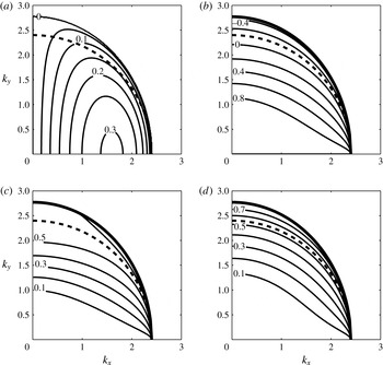
the circle stretches to an ellipse. Figure 1(a) shows the growth rate (the imaginary part of
 $k_{x}c$
) as a function of
 $k_{x}$
and
 $k_{y}$
for
 ${\it\epsilon}=1/2$
(
 $\mathit{Ri}=4$
). The thick outermost line is the marginal curve (the curve where the growth rate is zero), and the dashed line shows the marginal curve in the QG limit
 ${\it\epsilon}\rightarrow 0$
. Because the growth rate of a perturbation in the BEs is equal to the growth rate of a perturbation with smaller
 $k_{y}$
in the QG approximation, the growth rates in the BEs are larger than in QG.
Eady problem in the BEs with
 $\mathit{Ri}=4$
and
 ${\it\epsilon}=1/2$
. (a) Contours of non-dimensional growth rate (imaginary part of
 $k_{x}c$
); contour interval is 0.05. (b) Ratio of geostrophic baroclinic production to total energy production; contour interval is 0.2. (c) Ratio of ageostrophic baroclinic production to total energy production; contour interval is 0.1. (d) Ratio of shear production to total energy production; contour interval is 0.1. The dashed contour in all panels shows the marginal curve (zero growth rate) for the QG limit
 ${\it\epsilon}\rightarrow 0$
, and the thick outermost curve in (b–d) shows the marginal curve for the BEs.

The increased growth rate compared to QG off the
 $k_{y}=0$
axis results from the extra extraction of energy from the large scales by the perturbations as a result of ageostrophic baroclinic production and shear production in (2.19). To confirm this effect, the perturbation energy production terms in (2.19) are computed for a range of wavenumbers at
 $\mathit{Ri}=4$
.
The ageostrophic velocity potential
 ${\it\phi}^{\prime }$
is determined from (2.30) as
 $$\begin{eqnarray}{\it\Phi}=\frac{\text{i}k_{x}\text{e}^{-{\it\epsilon}\text{i}k_{y}z}}{{\it\kappa}^{2}}[C_{1}({\it\kappa}z\text{e}^{{\it\kappa}z}+(1+c{\it\kappa})(1-\text{e}^{{\it\kappa}z}))-C_{2}({\it\kappa}z\text{e}^{-{\it\kappa}z}-(1-c{\it\kappa})(1-\text{e}^{-{\it\kappa}z}))].\end{eqnarray}$$
Since this is a linear problem, the amplitude of the perturbations is arbitrary, making it difficult to compare the raw production terms for perturbations with different wavenumbers. To analyse the relative contribution of the three production terms at each wavenumber, each term is normalized by the total production rate. The normalized geostrophic baroclinic production (2.24), ageostrophic baroclinic production (2.25) and shear production (2.26) are shown in figure 1(b–d), respectively. The thick outermost line in each panel is the marginal curve (the curve where the growth rate is zero), and the dashed line shows the marginal curve in the QG limit
 ${\it\epsilon}\rightarrow 0$
.
Figure 1(b) shows that the geostrophic baroclinic production actually becomes negative for a range of unstable wavenumbers, including wavenumbers that would be unstable in the QG approximation. As a result, the remaining terms must be positive, since a mode cannot be unstable and have a negative energy production. Indeed, figure 1(c,d) shows that the ageostrophic baroclinic production and shear production make major contributions to the instability of small-scale modes where the geostrophic baroclinic production is negative. For modes with small cross-front variation (small
 $k_{y}$
) these terms are small.
In the QG approximation the velocity is orthogonal to
 $(k_{x},k_{y})$
, and only the
 $k_{x}$
component can extract potential energy from the large-scale flow. As a result, modes with non-zero
 $k_{y}$
are less efficient at extracting energy from the large scales, and have smaller growth rates. In the BEs the velocity includes an ageostrophic component parallel to
 $(k_{x},k_{y})$
. As a result, the ageostrophic velocity is able to contribute to the extraction of large-scale potential energy, leading to higher growth rates. Similarly, the vertical velocity in QG is too small to be able to extract kinetic energy from the large-scale flow through shear production. In the BEs the vertical velocity is larger, and the perturbations are able to extract kinetic energy through shear production.
Although the BEs are more accurate than QG for submesoscale dynamics, they are still imperfect approximations of the balanced dynamics, as demonstrated by the fact that they miss the ageostrophic effects on the
 $k_{y}=0$
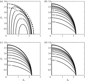
modes found by Stone (Reference Stone1966). For comparison with the BE results, the growth rates and energy production terms for the Eady problem in the hydrostatic primitive equations are shown in figure 2. The linear perturbation equations for the hydrostatic equations are reviewed in appendix A. As expected, the growth rates and range of unstable modes with
 $k_{y}=0$
are diminished in the primitive equations compared to the BEs. However, the marginal curve for the BEs (dash-dotted in figure 2
a) smoothly joins the primitive-equation curve for larger
 $k_{y}$
. The qualitative properties of the perturbation energy budgets are overall quite accurate in the BEs: there is a range of modes with negative geostrophic baroclinic production, and ageostrophic baroclinic production and shear production contribute in nearly equal parts to modes with moderate
 $k_{y}$
. Although the details of the BE energy budget are not exactly correct, the conclusions from the BE analysis are in fact exaggerated in the primitive equations: for modes with large
 $k_{y}$
the ageostrophic baroclinic and shear production play a larger role than in the BEs.
Eady problem in the hydrostatic primitive equations with
 $\mathit{Ri}=4$
and
 ${\it\epsilon}=1/2$
. Panels (a–d) are the same as in figure 1, with the same contour intervals. The dashed contour in (a) shows the marginal curve (zero growth rate) for the QG limit
 ${\it\epsilon}\rightarrow 0$
, and the dash-dotted contour shows the marginal curve for the BEs. The outermost solid contour in all panels shows the location where the primitive-equation growth rate is
 $5\times 10^{-4}$
, which is a proxy for the marginal curve.

4. Variable stratification
The Eady problem is attractive for its simplicity, but it may not provide a very accurate model of submesoscale baroclinic instability in the ocean mixed layer, e.g. because the shear and stratification are not constant and the bottom of the mixed layer is not rigid. The goal of this section is to verify that the qualitative properties of the Eady problem are present in a more realistic scenario. In order to stay within the framework of § 2, the shear is kept constant and the buoyancy frequency is allowed to vary with depth. To increase the level of realism as compared to the Eady problem, the buoyancy frequency is modelled as an increasing function of depth, mimicking the increase of stratification at the base of the mixed layer. The stratification is chosen so that the large-scale potential vorticity gradient
 $\partial _{y}Q$
in the QG problem is constant (see (2.36)), which results in the following profile:
 $$\begin{eqnarray}N^{2}(z)=\frac{1+{\it\delta}}{z+{\it\delta}},\end{eqnarray}$$
where
 ${\it\delta}$
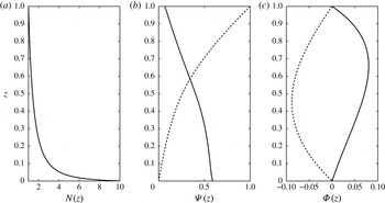
is a tunable parameter. The buoyancy frequency attains a minimum at the top of the mixed layer, and increases nonlinearly with depth; an example with
 ${\it\delta}=1/99$
is shown in figure 3(a). The use of a uniform large-scale potential vorticity gradient makes this scenario loosely analogous to the atmospheric Charney problem since it satisfies a similar necessary condition for instability, namely that the sign of the surface shear is opposite to the sign of the interior potential vorticity gradient (Vallis Reference Vallis2006).
(a) Plot of
 $N(z)$
from (4.1) with
 ${\it\delta}=1/99$
. (b,c) Vertical profiles of the real (solid) and imaginary (dashed) parts of
 ${\it\Psi}$
and
 ${\it\Phi}$
, respectively, for the most unstable mode.

Although the normal mode equations for this scenario (2.33) are exactly solvable in terms of hypergeometric functions, the resulting formulas are relatively opaque, so the instability problem is analysed numerically using
 ${\it\delta}=1/99$
and
 ${\it\epsilon}=1/\sqrt{2}$
. Specifically, the normal mode equation (2.33) is discretized on a Chebyshev pseudospectral grid with 257 points (Trefethen Reference Trefethen2000) and the resulting linear system is solved as a generalized eigenvalue problem for
 ${\it\Psi}$
and
 $c$
. The ageostrophic streamfunction
 ${\it\Phi}$
is determined from (2.31).
Figure 3(a) shows the structure of
 $N(z)$
from (4.1) with
 ${\it\delta}=1/99$
; the buoyancy frequency increases by a factor of 10 from the top to the bottom of the layer. The linear instability problem is solved numerically with
 ${\it\epsilon}=1/\sqrt{2}$
, which implies that the Richardson number increases from 2 at the top of the layer to 200 at the bottom of the layer. The most unstable mode occurs for
 $k_{x}\approx 1.26$
and
 $k_{y}=0$
, as in the QG problem, and has a vertical structure independent of the Richardson number. The horizontal scale appears slightly larger than the Eady problem, which has most unstable mode at
 $k_{x}\approx 1.6$
, but this is primarily because the non-dimensional deformation radius is larger here than in the Eady problem owing to the increase of
 $N$
with depth. Figure 3(b,c) shows the vertical structure of
 ${\it\Psi}$
and
 ${\it\Phi}$
for the most unstable mode; the real parts are solid and the imaginary parts are dashed.
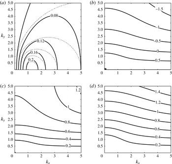
Figure 4(a) shows the growth rate of the linear instability in the BEs for a range of
 $k_{x}$
and
 $k_{y}$
; the growth rate in the QG problem (
 ${\it\epsilon}\rightarrow 0$
) is shown using dotted contours for comparison. Non-QG effects are felt only by modes with
 $k_{y}\neq 0$
– so the contours of growth rate match up on the
 $k_{x}$
axis – and, as in the Eady problem, the balanced ageostrophic effects contribute to an increased level of instability for modes with
 $k_{y}\neq 0$
.
Ocean mixed layer Charney problem in the BEs with constant shear and
 ${\it\epsilon}=1/\sqrt{2}$
. (a) Contours of non-dimensional growth rate (imaginary part of
 $k_{x}c$
) for the BE (solid) and QG (dotted) equations; contour interval is 0.04. (b) Ratio of geostrophic baroclinic production to total energy production; contour interval is 0.5. (c) Ratio of ageostrophic baroclinic production to total energy production; contour interval is 0.2. (d) Ratio of shear production to total energy production; contour interval is 0.2.

As in the Eady problem, the increased growth rate in the BEs can be attributed to baroclinic production and shear production by the ageostrophic velocity. Figure 4(b–d) shows the rates of geostrophic baroclinic production (2.24), ageostrophic baroclinic production (2.25) and shear production (2.26) normalized by the net production. As in the Eady problem, the geostrophic production is positive and dominates for modes with small
 $k_{y}$
, but actually becomes negative for a range of modes with moderate
 $k_{y}$
, where the ageostrophic velocity is driving the instability through both baroclinic and shear production. The ageostrophic baroclinic production and shear production contribute almost equally to the net production at all wavenumbers, with slightly more shear production for small
 $k_{x}$
and larger
 $k_{y}$
.
5. Conclusions
Submesoscale baroclinic instability in the ocean mixed layer is an important process responsible for re-stratification of the mixed layer (Boccaletti et al. Reference Boccaletti, Ferrari and Fox-Kemper2007). At the relatively small horizontal scales of the submesoscale mixed layer dynamics, of the order of 1–10 km, the QG approximation is not appropriate and ageostrophic effects significantly affect the dynamics (Capet et al. Reference Capet, McWilliams, Molemaker and Shchepetkin2008). Analytical investigations of ageostrophic effects in baroclinic instability typically proceed from the primitive equations (an exception being Blumen (Reference Blumen1980)), which complicates the analysis because it includes unbalanced modes of instability like the symmetric and Kelvin–Helmholtz instabilities (Stone Reference Stone1966). The present approach makes use of the BEs (McWilliams & Gent Reference McWilliams and Gent1980), which include ageostrophic effects beyond the QG approximation while eliminating the unbalanced instabilities. A major drawback of the BEs for baroclinic instability is that the linearized perturbation equations have coefficients varying with the horizontal coordinates unless the baroclinic shear is constant (see § 2). The present analysis is therefore restricted to constant shear. Also, the BEs do not include the unbalanced baroclinic instability studied by Molemaker, McWilliams & Yavneh (Reference Molemaker, McWilliams and Yavneh2005).
Analysis of the BE linear baroclinic instability problem in § 2 shows that the instability of perturbations with no cross-front variation (i.e. normal modes with
 $k_{y}=0$
) is the same as in the QG problem. This indicates that there are additional balanced ageostrophic effects in baroclinic instability that are not captured by the BEs, since Stone (Reference Stone1966) showed that modes with
 $k_{y}=0$
respond to ageostrophic effects. Section 2 also shows that there are three kinds of perturbation energy production in the BE baroclinic instability problem: geostrophic and ageostrophic baroclinic production, and shear production. Baroclinic production of perturbation energy is a sine qua non of baroclinic instability, but shear production is more commonly associated with unbalanced instabilities like the symmetric and Kelvin–Helmholtz instabilities.
Section 3 solves the Eady problem (constant shear, constant buoyancy frequency) analytically using the BEs. The range of unstable modes is extended for perturbations with cross-front variation, and it is verified that this increased instability results from both of the ageostrophic perturbation energy production terms: ageostrophic baroclinic production and shear production. In fact, there is a range of unstable modes that have negative geostrophic baroclinic production that is countered only by shear and ageostrophic baroclinic production. The importance of ageostrophic perturbation energy production is qualitatively verified by comparison with the hydrostatic primitive equations, although additional ageostrophic effects reduce the range of unstable modes with no cross-front variation.
The Eady problem is not the most accurate approximation to the ocean mixed layer, e.g. because the stratification in the ocean is not uniform and the base of the mixed layer is not rigid. To test whether the qualitative results of the Eady problem are retained in more realistic situations, § 4 numerically investigates the baroclinic instability of a layer of fluid with buoyancy frequency that increases sharply near the lower boundary, mimicking the base of the ocean mixed layer. As with the Eady problem, the ageostrophic perturbation energy production terms have a significant impact on perturbations with cross-front variation; the results of the Eady problem suggest that there may be additional ageostrophic effects not captured by the BEs that act primarily on perturbations with no cross-front variation.
In summary, the BEs are used to show that balanced ageostrophic effects make significant contributions to the energetics of perturbations in linear baroclinic instability, and in particular that shear production is a significant source of energy for perturbations with non-zero cross-front variation. Although the most unstable mode in the BE analysis is exactly the same as in the QG analysis, perturbations with cross-front variation have faster growth rates. The results suggest that submesoscale baroclinic instability in the ocean mixed layer extracts both kinetic and potential energy from geostrophic fronts by simultaneously flattening isopycnals and eroding the associated geostrophic shear. As always, there is a gap between linear instability theory and the nonlinear evolution of real ocean dynamics, but one hopes that the linear analysis will provide at least a qualitative guide in helping to understand the more complex evolution of submesoscale baroclinic instability in the ocean mixed layer.
Acknowledgements
The author’s interest in submesoscale baroclinic instability and the balance equations was sparked by a reading group at the Courant Institute in 2012–2013 organized by K. S. Smith and S. R. Keating.
Appendix A. The primitive-equation Eady problem
The non-dimensional linear perturbation equations for the Eady problem in the hydrostatic primitive equations are
 $$\begin{eqnarray}\displaystyle & (\partial _{t}+z\partial _{x})\boldsymbol{u}^{\prime }+{\it\epsilon}w^{\prime }\hat{\boldsymbol{x}}+{\it\epsilon}^{-1}\hat{\boldsymbol{z}}\times \boldsymbol{u}^{\prime }=-{\it\epsilon}^{-1}\boldsymbol{{\rm\nabla}}p^{\prime }, & \displaystyle\end{eqnarray}$$
 $$\begin{eqnarray}\displaystyle & (\partial _{t}+z\partial _{x})b^{\prime }-v^{\prime }+w^{\prime }=0, & \displaystyle\end{eqnarray}$$
 $$\begin{eqnarray}\displaystyle & \boldsymbol{{\rm\nabla}}\boldsymbol{\cdot }\boldsymbol{u}^{\prime }+{\it\epsilon}\partial _{z}w^{\prime }=0, & \displaystyle\end{eqnarray}$$
 ${\it\epsilon}={\it\Lambda}/N$
. The perturbation energy equation is
 $$\begin{eqnarray}\frac{1}{2}\frac{\text{d}}{\text{d}t}\langle |\boldsymbol{u}^{\prime }|^{2}+(b^{\prime })^{2}\rangle =-{\it\epsilon}\langle w^{\prime }u^{\prime }\rangle +\langle v^{\prime }b^{\prime }\rangle .\end{eqnarray}$$
The non-dimensional velocities are written in terms of poloidal and toroidal potentials as
 $$\begin{eqnarray}u^{\prime }=-\partial _{y}{\it\psi}-{\it\epsilon}\partial _{xz}{\it\phi},\quad v^{\prime }=\partial _{x}{\it\psi}-{\it\epsilon}\partial _{yz}{\it\phi},\quad w={\rm\nabla}_{h}^{2}{\it\phi}.\end{eqnarray}$$
The perturbation equations (A 1)–(A 3) may be written in terms of the velocity potentials as
 $$\begin{eqnarray}\displaystyle & (\partial _{t}+z\partial _{x}){\it\psi}-{\it\epsilon}\partial _{y}{\it\phi}-\partial _{z}{\it\phi}=0, & \displaystyle\end{eqnarray}$$
 $$\begin{eqnarray}\displaystyle & (\partial _{t}+z\partial _{x})\partial _{z}^{2}{\it\phi}+{\it\epsilon}^{-2}\partial _{z}{\it\psi}-{\it\epsilon}^{-2}b=0, & \displaystyle\end{eqnarray}$$
 $$\begin{eqnarray}\displaystyle & (\partial _{t}+z\partial _{x})b^{\prime }-(\partial _{x}{\it\psi}-{\it\epsilon}\partial _{yz}{\it\phi})+{\rm\nabla}_{h}^{2}{\it\phi}=0. & \displaystyle\end{eqnarray}$$
 $w$
(Stone Reference Stone1966):
 $$\begin{eqnarray}(1-({\it\sigma}+k_{x}z)^{2})\frac{\text{d}^{2}w^{\prime }}{\text{d}z^{2}}-\left(\frac{2k_{x}}{{\it\sigma}+k_{x}z}-2\text{i}k_{y}\right)\frac{\text{d}w^{\prime }}{\text{d}z}-\left({\it\epsilon}^{-2}k^{2}+\frac{2\text{i}k_{x}k_{y}}{{\it\sigma}+k_{x}z}\right)w^{\prime }=0.\end{eqnarray}$$
Stone shows that there are no growing solutions on the symmetric axis (
 $k_{x}=0$
) for
 ${\it\epsilon}\geqslant 1$
(this is an exact solution). Note also that the condensed equation (A 9) is cubic in the growth rate
 ${\it\sigma}$
, whereas the BE counterpart, (2.27), is linear in the growth rate. This is because the BEs do not include inertio-gravity waves and their associated unbalanced instabilities.
Equations (A 6)–(A 8) are discretized using a Chebyshev pseudospectral method with 257 points in the vertical direction. The resulting generalized eigenvalue problem for the growth rate
 ${\it\sigma}$
is solved for a range of wavenumbers, and the results are used to generate figure 2, which is directly analogous to figure 1, and is discussed in § 3.