1 Introduction
Currently, it is often easy to find collections of documents covering a particular subject of a general domain. For example, when studying Physics a student can use search engines to gather several documents from the various subjects he needs to study (for example, kinematics and frictional forces). This includes different documents from the same subject. Moreover, documents from different media sources, such as textbooks or video lectures, can also be obtained. From a pedagogical perspective, this can be very useful, as different documents may offer complementary views about the same subject, and, thus, help students with different learning needs. However, as observed by Shahaf, Guestrin and Horvitz (Reference Shahaf, Guestrin and Horvitz2012), if search engines are effective in retrieving these collections, the task of putting them into a coherent picture remains a challenge. This is because search engines only retrieve a list of documents and navigating all their raw content is cumbersome. For example, a student at some point might be focused on the topic of acceleration, from the kinematics subject, and have difficulty in finding it in a 2-hour video lecture. This problem can be addressed by providing a better structuring of the documents. Documents exhibit a content organization which aggregates related text passages (e.g., sentences or paragraphs) into topic segments, such as the one in the previous example. As suggested by Minwoo and Ivan (Reference Minwoo and Ivan2010), linking topically related segments from different documents could help to construct friendlier user interfaces. However, before moving to the linking step, documents need to be segmented by topic.
Topic segmentation (Choi Reference Choi2000; Galley et al. Reference Galley, McKeown, Fosler and Jing2003; Purver et al. Reference Purver, Griffiths, Körding and Tenenbaum2006; Eisenstein and Barzilay Reference Eisenstein2009; Kazantseva and Szpakowicz Reference Kazantseva and Szpakowicz2011; Nguyen et al. Reference Nguyen, Boyd-Graber, Resnik, Cai, Midberry and Wang2014; Shah et al. Reference Shah, Yu, Shaikh, Tang and Zimmermann2014) is a well-established research area. The automatic recovery of topic boundaries is traditionally based on the content of isolated documents. Recently, Minwoo and Ivan (Reference Minwoo and Ivan2010) and Mota, Eskenazi and Coheur (Reference Mota, Eskenazi and Coheur2016) proposed new segmentation models, respectively, MultiSeg and BayesSeg-MD models, in which the segmentation of a document takes advantage of existing related documents (from now on, the multi-document approach), instead of segmenting a document based on its own content (from now on, single-document approach). The intuition is that the repeated discussion of the same topic (Figure 1), in several related documents, will lead to more accurate segment likelihood estimations (Mota et al. Reference Mota, Eskenazi and Coheur2016). Indeed, in this scenario of learning materials, segmenting one single document by topic might be a complicated task, as many of the vocabulary changes are not abrupt. Thus, looking at different documents on the same subject might help to identify the different topics. Another advantage is that the multi-document model approach also lends itself to exploring shared topic orderings of the segments (Du, Pate and Johnson Reference Du, Pate and Johnson2015), allowing a better overall segmentation to be obtained. The applicability of such models goes beyond the document topic segmentation scope, as other tasks can also benefit (Prince and Labadie Reference Prince and Labadie2007; Haghighi and Vanderwende Reference Haghighi and Vanderwende2009; Shah and Zimmermann Reference Shah and Zimmermann2017). For example, Watanabe et al. (Reference Watanabe, Iwata, Hori, Sako and Ariki2011) perform automatic transcription of video lecture audio. The audio is split using a fixed length window and individual language models are calculated for each obtained segment. If multi-document models are used, one can expect to obtain higher quality language models, since these are estimated through the optimal segmentation instead of a (non-informative) fix window.
Examples of segment excerpts from Video, PowerPoint (PPT), and PDF documents, respectively, in the acceleration topic. Words in bold depict the shared vocabulary across segments, which can be used to leverage segmentation in multi-document models.

In order to evaluate multi-document models, a reasonable amount of documents about the same subject needs to be available. In addition, and considering a real scenario, different media sources should be included in such a collection. Minwoo and Ivan (Reference Minwoo and Ivan2010) evaluate their multi-document model in a variety of subjects, but, except in one case, there are few documents per subject (in some cases, only two documents). Mota and his colleagues (Reference Mota, Eskenazi and Coheur2016) propose a new dataset with multimedia related learning materials, but only ten documents from a single subject are available. None of these authors report any type of annotators’ agreement.
We fill this gap with MUSED (Figure 1). MUSED is a dataset shaped to simulate a real scenario, in which someone needs to study some subjects in the Physics domain, and gathers from the web several multimedia documents (web pages, presentations, textbooks, videos, etc.) about each subject. Seven subjects are considered, as well as around twenty documents per subject, in a total of 141 multimedia documents, manually segmented. In total, there are 739 segments, the average number of segments per document is five and the average length of the segments is 490 words.Footnote 1
In this paper, we describe the manual segmentation process and discuss the use of certain and uncertain boundaries. We also calculate an inter-annotator agreement, which is higher than the ones reported in related tasks. Moreover, we benchmark MUSED with available segmentation models (both single- and multi-document). We also study how existing models behave in the presence of different media sources. We show that multi-document models still need to be improved in order to surpass the results obtained by single-document models and that some techniques are sensitive to different media sources.
This paper is organized as follows: In Section 2, we present related work. In Section 3, we describe MUSED, and, in Section 4, we run several experiments. Finally, in Section 5, we present main conclusions and point to future work.
2 Related work
This section describes well-known topic segmentation models, as well as the available datasets for this task.
2.1 Topic segmentation datasets
Research in topic segmentation has mainly focused on the single document case, for which several datasets exist. The problem is that these datasets are not suitable for evaluating multi-document segmentation. This is because multi-document segmentation models assume that the same topics are discussed in several different documents. The datasets for single document segmentation do not have this property. Although they might have an overarching domain, the topics discussed in the segments are inherently different. For example, Malioutov and Barzilay (Reference Malioutov and Barzilay2006) provide a dataset in the Physics domain. Despite all documents being in the same overarching domain, the subjects are different. For example, the topics described in the segments from the ‘Hooke’s Law’ subject are not the same as in the ‘Work and Energy’ subject (the following lesson). Therefore, the segments describe different topics as well. What is needed for evaluating multi-document segmentation are documents describing similar topic segments, which we refer as related documents. It should be noted that this neither implies that all documents have all topics, nor that they are all described at the same level of detail.
Choi (Reference Choi2000) developed an artificial dataset by putting together the first n sentences from different and unrelated documents in the Brown corpus (Francis and Kucera Reference Francis and Kucera1979). This corpus contains documents from 500 sources categorized by genre, such as news. The documents are also categorized by domain (politics, sports, society, etc.). In total, 700 artificial documents were generated, each with ten segments, and using a value of n ranging between three and eleven. The problem with this dataset is that topic boundaries can be easily detected since the shifts in words distributions are abrupt. Thus, the dataset does not capture the topic development aspect where word usage changes smoothly.
The ICSI multi-party meeting dataset (Janin et al. Reference Jain and Neal2004) consists of meetings from various research groups (for instance, there are research groups on natural language processing and internet architectures). In total, the dataset contains seventy five meeting transcripts, of which twenty five were manually segmented. The average number of identified segments per documents is five. ICSI does not have a specific domain, thus, it is hard to find related documents. The problem with this dataset is that the meetings mostly discuss ongoing research projects for which is hard to find related documents. For instance, the meetings of the natural language processing group concern the building of the ICSI dataset itself. Later, Hsueh, Moore and Renals (Reference Hsueh, Moore and Renals2006) extended the annotations in this dataset to further divide the existing segments into finer-grained topics, but the problem remains.
Kazantseva and Szpakowicz (Reference Kazantseva and Szpakowicz2011) provided a dataset with twenty five chapters from a XIX century novel, The Moonstone by Wilkie Collins. The chapters have an average length of 53.85 paragraphs, with an average of 5.8 segments each, and were annotated by groups between four and six annotators. Annotators were instructed to segment the chapters into episodes, in order to create an outline for the chapter. This domain is not suitable to be extended for a multi-document segmentation since it is also not easy to find related documents.
In an educational setting, Eisenstein (Reference Eisenstein2009) used a medical textbook (Walker, Dallas and Willis Reference Walker, Dallas and Willis1990) to evaluate topic segmentation. The goal was to the divide each chapter into their individual sections. This dataset contains 227 chapters, with 1,136 sections (an average of five per chapter). Each chapter contains an average of 140 sentences, giving an average of twenty eight sentences per segment. No related documents are available in this corpus.
Also in the educational setting, Malioutov and Barzilay (Reference Malioutov and Barzilay2006) provided two lecture datasets in the domains of Artificial Intelligence (twenty two lectures with 5.9 segments in average) and Physics (thirty three lectures with 12.3 segments in average). Considering the former, topic boundaries in each video transcript were based on the slide changes occurring in the video. Therefore, these boundaries may not correspond to topics. In the latter case, documents were manually segmented by four annotators. In both cases, each lecture has its own domain, thus, multi-document topic segmentation models cannot be evaluated using this data.
The Similar Segments in Social Speech task, in the MediaEval campaign (Ward et al. Reference Ward, Werner, Novick, Shriberg, Oertel and Kawahara2013), provided a corpus with topically related segments. The task is defined as receiving an audio segment of interest and returning an ordered list of jump-in points for regions similar to it. By doing so, whenever a relevant piece of information is found, other related information can also be accessed efficiently. For this purpose, a corpus of dialogs among university students was created. The dataset has twenty six dialogs with 309 minutes in total (1,697 segments). Dialogs were annotated by four annotators, though the same dialog was not annotated by more than one annotator. What makes the Similar Segments in Social Speech corpus unsuitable for multi-document segmentation is that there is no general subject in the individual documents (for example, the same document can talk about internships, family, movies, etc.). This is the same issue described in Choi’s dataset.
Joty, Carenini and Ng (Reference Joty, Carenini and Ng2013) studied topic segmentation and labeling in a dataset of asynchronous conversations, that is, conversations that do not require right-now attention. The provided dataset contains forty email threads from the World Wide Web Consortium with an average number of 2.5 topics per thread. Although each email thread has repeated discussions of the same topic, several unrelated topics also occur in a single thread. This has the same pitfalls identified in both Similar Segments in Social Speech and Choi’s datasets: Segments can be easily distinguished, which do not allow an accurate evaluation of segmentation models. In addition, the dataset contains twenty conversations, with an average of 10.8 topics each, from the technology-related news website Slashdot. In this domain, a document corresponds to the sequence of comments made by users regarding a news article. This scope is much different from the one we want to target with MUSED: how documents describing in detail some subject are structured.
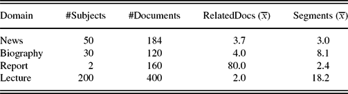
Considering multi-document models, the datasets used to evaluate them have several limitations. Multiseg (Minwoo and Ivan Reference Minwoo and Ivan2010) was evaluated in four different domains: news, biography, report, and lecture. To create the News domain, document clusters were collected from the science and technology section in news.google.com. For the Biography domain, four websites were used as source en.wikipedia.org, simple.wikipedia.org, biography.com, and notablebiographies.com. The Report domain consists of reports describing a plant growth lab, an assignment for a biology class (Sun et al. Reference Frey and Dueck2007). The Lecture domain, corresponds to the English as a second language podcast (Noh et al. Reference Noh, Jeong, Lee, Lee and Lee2010). Each episode consists of two parts: a story and an explanatory lecture discussing the meaning and usage of English expressions appearing in the story. The goal was to divide the lecture transcript into discourse units (i.e. focused paragraphs of the lecture). Table 1 provides statistics for each individual domain. Despite the high number of documents, it is important to notice that what we care about the most is the number of documents per subject (RelatedDocs column). In this perspective, each subject has, in fact, few documents. The only exception is the Report domain, but in it, the number of segments per document is very low.
Detailed description of the dataset from Minwoo and Ivan (Reference Minwoo and Ivan2010)

The symbol x indicates an average.
Finally, the dataset used to evaluate BayesSeg-MD (Mota et al. Reference Mota, Eskenazi and Coheur2016) has learning materials from different media sources (presentation, video lectures, and Wikipedia articles) on the subject of Adelson–Velsky and Landis’ trees. The main limitation of the dataset is its size, ten documents (manually segmented by a single annotator). The average number of segments per document is 8.3.
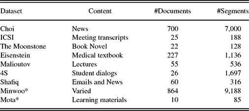
Table 2 summarizes some data regarding the surveyed datasets. Contrary to all these datasets, MUSED was tailored for testing (multi-)segmentation models in collections of related documents from different media sources. As previously mentioned, MUSED is comprised of 141 documents in seven different subjects in the Physics’ domain. MUSED has around twenty documents per subject, with an average number of five segments per document in a total of 739 segments, which makes it larger than the other datasets, apart from Choi’s, Eisenstein, and Minwoo datasets. However, Choi’s dataset is artificially generated, the 227 documents from Eisenstein are the chapters of a single book, Minwoo’s dataset is composed of documents on four different domains that either do not have a high number of related documents or the number of segments is low (the Report dataset).
Description of existing datasets with document segmentations

Datasets marked with ‘*’ can be used for multi-document segmentation evaluation.
2.2 Topic segmentation models
The following sections describe the state-of-the-art in the research area of topic segmentation. We start by describing single-document models (Section 2.2.1) and then multi-document models (Section 2.2.2).
2.2.1 Single-document models
Topic segmentation models are based on the Lexical Cohesion Theory (Halliday and Hasan Reference Halliday and Hasan1976). This theory postulates that discourse structure is tightly connected to the use of a cohesive vocabulary. Thus, topic segments can be identified by detecting vocabulary changes. The main difference between segmentation methods is how lexical cohesion is implemented: some resort to lexical similarity; the remaining follow a probabilistic approach.
The ones that resort to lexical similarity rely on a similarity metric, usually the cosine, calculated between sentences in a document. In this category, we find the following approaches:
• TextTiling (Hearst Reference Hearst1997), which slid a window across a document and computed the similarity between consecutive windows, creating a similarity plot. Topic segments were identified by finding the minimum values in the plot. Several works built on this idea (as for instance, the works described in Galley et al. (Reference Galley, McKeown, Fosler and Jing2003), Balagopalan and Damodar (Reference Balagopalan and Damodar2012), Shah et al. (Reference Shah, Yu, Shaikh, Tang and Zimmermann2015)).
• C99 (Choi Reference Choi2000), which used a ranked similarity matrix, and a divisive clustering approach to obtain segments. A local similarity context was employed, instead of relying on pairwise similarity measures (as in TextTiling). More recently, a new similarity metric, Content Vector Segmentation, based on the average value of the word embeddings of a segment, is used in the C99 algorithm (Alemi and Ginsparg Reference Alemi and Ginsparg2015).
• MinCut (Malioutov and Barzilay Reference Malioutov and Barzilay2006), which casted segmentation in a minimum cut graph partitioning problem. Graph representations of documents were obtained by creating a node for each sentence, edges were weighted according to their lexical similarity. This took the idea of local context in C99 further since long-distance relationships were encoded in the graph.
• Affinity Propagation Segmentation (APS) (Kazantseva and Szpakowicz Reference Kazantseva and Szpakowicz2011) also modeled long distances relationships, but by using Affinity Propagation clustering (Frey and Dueck Reference Frey and Dueck2007). The idea was to create a factor graph based on a similarity matrix and maximize a function corresponding to the sum of the similarities of the segments.
Other lexical cohesion strategies make use of topic modeling approach:
• Utiyama and Isahara (UI) (Utiyama and Isahara Reference Utiyama and Isahara2001) used language modeling to define the cost of a segmentation. The goal of this approach was to find compact language models that explained the different segments.
• BayesSeg (Eisenstein and Barzilay Reference Eisenstein and Barzilay2008) offered a generalization of the previous model using a Bayesian framework by considering sentences as draws from a multinomial language model. Similarly to UI, the goal was to find the segmentation that provides the highest possible likelihood. To avoid searching the full space of language models, a marginalization process was carried out based on the Dirichlet Compound Multinomial distribution (Johnson, Kotz and Balakrishnan Reference Johnson, Kotz and Balakrishnan1997). The Dirichlet Compound Multinomial expresses the expectation over all multinomial language models when conditioning on a Dirichlet prior. After the marginalization, it is possible to carry out a search that only takes place in the segmentation space. The best solution was found by resorting to a dynamic programming algorithm.
• PLDA (Purver et al. Reference Purver, Griffiths, Körding and Tenenbaum2006) was an adaptation of Latent Dirichlet allocation to topic segmentation. Similarly to Latent Dirichlet allocation, a topic proportions variable, modeled as a Multinomial distribution, determined the topic assignments made to the words in a document. In turn, topics were Multinomial distributions over the possible words in the vocabulary. This contrasts with BayesSeg, where each segment was modeled as being generated from a single topic. To obtain a segmentation, PLDA assigned a binary topic shift variable is to each sentence. Therefore, instead of computing topics and topic proportions at the document collection level, they were determined according to the segments of a single document. The only observable variables in the model are the words, the remaining – topics, topics proportions, and segments – correspond to latent structures. These were inferred using a Bayesian approach.
• Structured Topic Model (Du, Buntine and Johnson Reference Du, Buntine and Johnson2013) further developed PLDA by adding an extra Dirichlet distributed variable to sample the topic segment proportions. The intuition is that topics segment proportions are variations of the document topic segment proportions. This captures how the segment topic proportions of a document are related to each other, instead of being independently generated. Another advantage of Structured Topic Model is that the generative process was governed by a non-parametric Bayesian framework, thus, a number of topics do not need to be specified a priori. Models such as TopicTiling (Riedl and Biemann Reference Riedl and Biemann2012) and NTSeg (Jameel and Lam Reference Jameel and Lam2013) extended this research line.
2.2.2 Multi-document models
To the best of our knowledge, only two models, both following a probabilistic approach, target multi-document segmentation:
• MultiSeg (Minwoo and Ivan Reference Minwoo and Ivan2010) is a model in the same spirit to PLDA. The key differentiating aspect is that documents are assumed to have been generated by two types of topics, namely, local and global topics. Local topics are specific to a document, global topics are shared among documents. In practice, this was implemented as a two-level Latent Dirichlet allocation model, one for each type of topic. In this context, local topics were calculated based on topic assignments made in an individual document, whereas global topics were calculated based on the whole document collection. Given this dynamic between local and global topics, each sentence in the document collection was associated with a binary variable that indicates if the sentence was generated by a local or a global topic. Another difference between MultiSeg and other probabilistic approaches is that the actual segmentation is determined by changes in topic assignments. The number of topics is managed using a Bayesian non-parametric approach, similarly to Structured Topic Model. The inference on the model is based on a split-merge algorithm (Jain and Neal Reference Jain and Neal2004), which relies on Metropolis–Hastings proposals to merge two segments into one or split an existing segment into two.
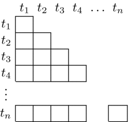
• BayesSeg-MD (Mota et al. Reference Mota, Eskenazi and Coheur2016) is an extension of BayesSeg that takes into account multiple documents. This was done by modifying the segment likelihood estimation in each step of the BayesSeg’s dynamic programming algorithm. The algorithm calculates all possible segmentation possibilities based on a matrix similar to the one depicted in Figure 2. Each (t i, t j) entry of the matrix corresponds to the likelihood of having a segment that begins on the t i sentence of a document and ends at the t j sentence. The algorithm works its way down the matrix, starting at the (t 1, t 1) entry. For each entry, it is necessary to track what was the previous segmentation with the highest likelihood. This is the dynamic programming aspect of the algorithm. For example, for entry (t 3, t 5), it is necessary to sum the likelihoods of the segment {t 3, t 4, t 5} with the highest likelihood segmentation of the previous sentences (t 1 and t 2). When calculating the segment likelihood in each matrix entry, BayesSeg-MD adds the word counts from the top-n most similar sentences (from other documents in the collection) to the Dirichlet Compound Multinomial distribution.
Fig. 2.Segment likelihood matrix used in the dynamic programming algorithm of BayesSeg.


To conclude, and despite the recent developments in topic segmentation, to the best of our knowledge, the evaluation of models targeting multi-document segmentation was only done in datasets that do not totally comply with the specificities of these models, as previously discussed. Therefore, in this work, we contribute with a new dataset capable of comparing single- and multi-document approaches. Moreover, there is no study that compares available segmentation models in the same dataset. In this paper, we benchmark available segmentation algorithms with MUSED.
3 Building MUSED
We now describe the process for building MUSED, as well as the carried out human segmentation study.
3.1 Collecting related documents
In order to have MUSED representing the needs of a real-world user, we adopt the scenario of a Physics’ student, who needs to read about different subjects in this domain. Therefore, he retrieves several (multimedia) documents covering those subjects from the web and briefly decides which ones should be part of the collection. Thus, we chose seven documents, with distinct subjects, from the Physics lectures dataset (Malioutov and Barzilay Reference Malioutov and Barzilay2006), to be used as seed documents, extending this way a dataset already validated by the topic segmentation community. This allows comparing the results of multi-document models with previous studies. The following documents were used:
• L02 - Introduction to Kinematics
• L03 - Vectors
• L06 - Newton’s Laws
• L08 - Frictional Forces
• L10 - Hooke’s Law
• L11 - Work and Energy
• L20 - Angular Momentum
Then, we gathered related documents from different media sources from the web, using a web scraping approach.Footnote 2 The approach consists in extracting keywords (Bougouin, Boudin and Daille Reference Bougouin, Boudin and Daille2013) from the seed document and submitting them to the following search engines: Google, Bing, Yahoo, and DuckDuckGo. Working from the top retrieved results down, and trying to balance the number of documents from each media as much as possible, around twenty related documents per subject were added to MUSED. All unrelated documents were discarded. The main content of the documents was extracted to a text file using available software.Footnote 3,Footnote 4,Footnote 5 In what concerns the videos, we extracted the corresponding subtitles.
3.2 Manual segmentation
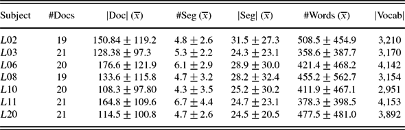
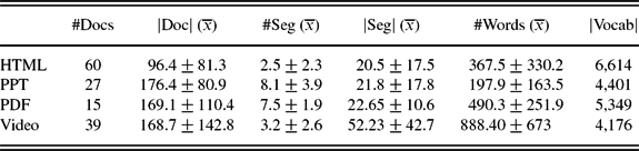
In a first step, the resulting set of documents was annotated by the first author, a researcher with a background in Computer Science. General rules of thumb provided in other studies (Galley et al. Reference Galley, McKeown, Fosler and Jing2003; Kazantseva and Szpakowicz Reference Kazantseva and Szpakowicz2012; Malioutov and Barzilay Reference Malioutov and Barzilay2006) were used, namely (a) segments should be cohesive and self-contained; (b) segments should contribute to the understanding of the content organization of the document. Statistics regarding the final MUSED dataset can be found in Tables 3 and 4 (dataset by domain and by media source, respectively), in which
• #Docs is the number of documents;
• |Doc| (x) is the average length of a document in sentences;
• #Seg (x) is the average number of segments per document;
• |Seg| (x) is the average length of a segment in sentences;
• #Words (x) is the average number of words per segment;
• |Vocab| is the length of the vocabulary.
MUSED dataset by domain

MUSED dataset by media source

In a second step, three more annotators were asked to annotate sixteen documents (four for each different media source) from the ‘Introduction to Kinematics’ and ‘Hooke’s Laws’ subjects. For each of these subjects, eight documents were annotated. One of the new annotators performed the annotations in all sixteen documents. The remaining two annotated eight documents each. Two of the new annotators also have a background in Computer Science and belong to the same research group as the first author, the other has a Mechanical Engineering background. For each subject, the annotators were given a deadline of two weeks to complete the annotation task. None of the annotators were monetarily compensated. Although the annotation was carried out in the text file version of the documents, a link to the original format (PPT, video, etc.) was provided. No particular order of the document was imposed to the annotators. Also, they were free to revise annotations before committing to a final segmentation.
Again, the guidelines closely followed the ones in previous human segmentation studies (Galley et al. Reference Galley, McKeown, Fosler and Jing2003; Malioutov and Barzilay Reference Malioutov and Barzilay2006; Kazantseva and Szpakowicz Reference Kazantseva and Szpakowicz2012), and focused on explaining the concept of a topic segment in a non-technical way.Footnote 6 Examples and counter-examples of document segmentations were provided. In addition, and similarly to Malioutov and Barzilay (Reference Malioutov and Barzilay2006), we asked annotators to provide a short description of each segment. The idea is that if it is hard to come up with a description or if the description is similar to the one in the previous segment, then, probably, the boundary should not exist. No expected number of segments was provided. Finally, we asked annotators to indicate if they were certain (or not) about the boundary annotation. This procedure has not been done in previous studies, but it incentivizes annotators to indicate segment boundaries in case of uncertainty. We consider that uncertainty in the annotation is related to annotators having doubts if their segmentation matches the target level of granularity. By investigating the role of uncertainty in the annotation process, we can better determine if annotators are converging to the same segmentation.
It should be mentioned that all the annotators referred that looking at the whole set of documents helped them to decide the boundary placement in each individual document.
3.3 Inter-annotator agreement
3.3.1 Agreement metrics
The most commonly used agreement coefficients are Krippendorff’s α (Krippendorff Reference Krippendorff2004), Cohen’s k (Cohen Reference Cohen1960), and Scott’s π (Scott Reference Scott1955). In this work, we use the multi-annotator version of π (Shrout and Fleiss Reference Shrout and Fleiss1979) (also known as Fleiss’s k), which is typically reported in segment annotation tasks (Hearst Reference Hearst1997; Passonneau and Litman Reference Passonneau and Litman1997; Kazantseva and Szpakowicz Reference Kazantseva and Szpakowicz2012; Fournier Reference Fournier2013). This coefficient is based on the observed agreement (A obs), corrected for chance by the expected agreement (A exp). The value of k Fleiss is 0 when there is no agreement, and 1 when there is complete agreement. It is calculated as follows:
 \begin{align}
k_{\text{Fleiss}} &= \frac{A_{\text{obs}} - A_{\text{exp}}}{1- A_{\text{exp}}}
\end{align}
 \begin{align}
A_{\text{obs}} &= \frac{1}{ic(c - 1)} \sum _{i \in I} \sum _{k \in K} n_{ik}(n_{ik} - 1)
\end{align}
 \begin{align}
A_{\text{exp}} &= \frac{1}{ic^2} \sum _{k \in K} n^2_k
\end{align}
• i is the number of items to be classified in the set I,
• k is the number of possible categories in K,
• c is the number of annotators,
• n k is the number of times category k was chosen by all annotators.
To calculate agreement, boundaries are considered labels, and their positions the decisions. Due to the difficulty of precisely defining a topic segment, it is common to find boundaries close to each other (near misses). Therefore, if a strict boundary match is required, the inter-coder agreement coefficient will underestimate the actual agreement. Thus, we use the modification of k Fleiss proposed by Fournier (Reference Fournier2013), which has been shown to more accurately estimate agreement than other methods. This approach uses the pairwise mean of the Boundary Edit Distance metric between annotators in the k Fleiss agreement coefficient. Boundary Edit Distance models segmentation differences using additions/deletions (full misses), and transpositions (near misses). A transposition occurs if the annotated boundaries are off by at most n sentences (this value is automatically estimated, and depends on the given data). A correctness score between 0 and 1 (the best value) is assigned depending on the number of boundary matches and edit operations needed to make the segmentations equal. The weight of the penalty depends on the type of edit operations. Additions and deletions provide higher penalties than transpositions. The penalty of transpositions is scaled based on the distance between the corresponding boundaries.
Another method for assessing inter-annotator agreement is to compute the pairwise Window Difference (WD) (Pevzner and Hearst Reference Pevzner and Hearst2002) of the annotations. WD slides a window through a document and penalizes segmentations according to the difference between the number of expected segments boundaries and the predicted ones. By doing so, partial credit is given to near-miss situations. This metric is calculated as follows:
 \begin{align}
WD = \frac{1}{N - k} \sum ^{N-k}_{i = 1} |\text{ref} - \text{hyp}| \ne 0\vspace*{-3.0pt}
\end{align}
3.3.2 Inter-annotator agreement results
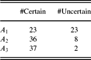
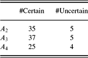
The number of obtained certain/uncertain boundaries for each individual annotator, for each subject, is presented in Tables 5 and 6. The second annotator, A2, was the one responsible for annotating the whole collection. In total, 240 segment boundaries were annotated, from which forty seven were marked as uncertain (19.6 per cent of the total).
Number of certain and uncertain annotations for L02 documents

Number of certain and uncertain annotations for L10 documents

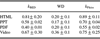
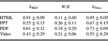
Considering that we have certain and uncertain boundaries, and in order to bring ‘crowd wisdom’ to the annotation process, uncertain boundaries marked by a single annotator were discarded. The intuition was the following: If only one annotator marks a boundary as uncertain, then it is plausible to assume that the boundary may not exist. On the other hand, if multiple annotators mark a boundary as uncertain, it is plausible to assume that it exists. Tables 7 and 8 show the inter-annotator agreement results using the previously described metrics, for each subject. For completeness, we also report the agreement results using the strict metric k Fleiss.
Inter-annotator agreement in L02 documents

Inter-annotator agreement in L10 documents

Despite the differences in the results between k BED and k Fleiss, ranging between 0.08 and 0.12, both metrics provide a similar view of the agreement obtained in the annotation tasks. What stands out from these results is that k Fleiss yield higher agreement than k BED when previous reports showed an opposite behavior (Fournier Reference Fournier2013). This is related to the fact that we removed uncertain boundaries annotated only once. Regarding the WD results, they do not completely agree on which is the hardest and easiest media to annotate when compared with the other agreement metrics. For example, in L02 the k BED results indicate that HTML documents obtained higher agreement and PDF the lowest. For WD, the highest agreement is obtained in PPTs and the lowest in Video transcripts documents, although the difference between PPT and HTML is only three per cent. Less ranking discrepancies were observed in the L10 case. Only the ranking of PPT and PDF is not consistent. On a manual qualitative analysis of the annotations, we observed that k BED better translates the agreement differences across media sources. This is in line with Fournier (Reference Fournier2013), where it is argued that WD overinflates its agreement results for sparse segmentations, which is indeed the case for documents that show inconsistencies across evaluation metrics. Another reason for the agreement differences is that the final WD is the average of the WD results for each pair of annotators, and k BED does micro-averages at the segment level, for all the annotators at the same time (and not pairwise).
k BED results are higher than the values reported in other datasets. In total, we obtained a 0.65 average agreement, whereas Fournier (Reference Fournier2013) and Kazantseva (Reference Kazantseva and Szpakowicz2011) obtained 0.44 and 0.30, respectively. A similar scenario is found when comparing WD results. We obtained a 0.21 average WD, which is better than the 0.35 in Janin, Ang, Bhagat, and Wrede (Reference Janin, Ang, Bhagat and Wrede2004) and 0.34 in Malioutov and Barzilay (Reference Malioutov and Barzilay2006). Some of the differences between our annotation task and the previous ones, which might explain the different results, are the nature of the target documents and how segments are annotated. MUSED is comprised of learning material documents which have a less ambiguous topic structure than the book chapters of the romance in Kazantseva (Reference Kazantseva and Szpakowicz2011). The annotation in MUSED is also simpler than the one in Malioutov and Barzilay (Reference Malioutov and Barzilay2006), which added extra cognitive load to the task by requiring major and minor topics to be identified. Despite providing detailed descriptions of what major and minor topics are, no concrete examples were given, as we did for MUSED.
Finally, and considering that A2 was the main annotator, responsible for annotating the whole dataset, we calculated his WD agreement with A1 (0.17±0.11), A3 (0.15±0.11), and A4 (0.14±0.14). In all cases, the WD score is low, suggesting that A2 consistently segmented the remaining documents.
3.3.3 Dealing with uncertainty
Previous results were calculated considering that uncertain boundaries marked by a single annotator are discarded (from now on the No Uncertainty Singleton (No-Single-U) scenario). In order to study the impact of uncertain boundaries, we conducted another study, in which two other scenarios were considered as follows:
• All Annotations (All): all boundaries (certain or uncertain) are considered.
• No Uncertainty (No-U): all uncertain annotations are discarded.
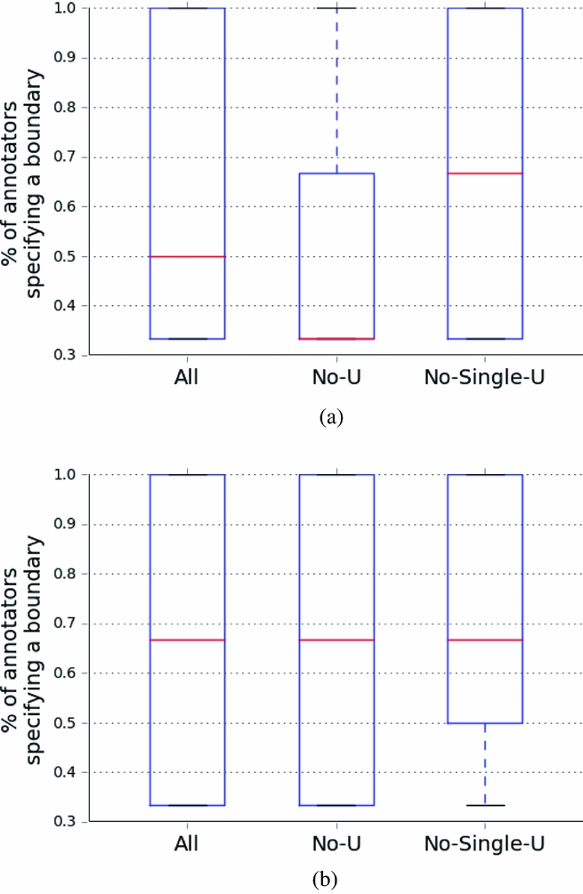
Figure 3 shows what percentage of annotators included a particular boundary in their segmentation for each version of the annotations dataset and each individual subject.
Box plots for the percentage of annotators assigning a topic boundary. (a) annotations of the L02 documents and (b) Annotations of the L10 documents.

For the L02 case (Figure 3(a)), we can see that the No-U scenario is the one with more disagreement among annotators, since most boundaries were annotated by thirty three per cent and sixty seven per cent of the annotators, and only in a few cases there is complete agreement. This result contrasts with the All and No-Single-U annotations, where a higher percentage exists, as most boundaries were annotated by two annotators. Moreover, a significant portion of the distribution has 100% agreement. The difference between All and No-Single-U is the median value. In No-Single-U, the median is sixty seven per cent, thus, there are more cases where at least two annotators specified a boundary.
The differences between the annotation datasets for L10 are not as prominent as before (Figure 3(b)). In all scenarios, a median value of sixty seven per cent was obtained. The difference is that the No-Single-U annotations do not have as many lower percentage values as the remaining. These different results in L02 and L10 suggest that some subjects might be harder to segment than others. This was hinted before when looking at the number of uncertain boundaries used in L02 and L10 (Tables 5 and 6). For the latter case, a much more varied number on uncertain boundaries was used, even though two of the annotators remained the same across subjects. This argues in favor of the proposed annotation scheme which allows a post-analysis of the annotations that better translates the actual agreement between annotators.
3.3.4 Qualitative analysis
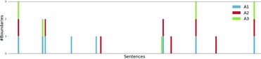
To better understand the disagreement patterns, Figure 4 shows a plot with the annotated boundaries in a PDF document with a low agreement (k BED = 0.4) from the L02 subject. Despite the low agreement, it is possible to observe that there is a set of boundaries for which all the three annotators agree (the vertical lines with three different colors). This indicates that some topical shifts are more prominent than others.
PDF document annotations in a document from the L02 subject.

Figure 4 also illustrates ‘near miss’ situations, in which the boundaries chosen by the annotators are close (the vertical lines with different colors are near to one another). This is due to the difficulty in perceiving if a text span is concluding the current segment or introducing the following one. This usually happens when a text span compares and contrast concepts from the previous and the next segments.
From Figure 4, it is also possible to see that different levels of granularity still exist in some annotations. Annotator A1 provided a finer level of granularity than the remaining ones. For example, he considered two different segments of ‘Average Velocity’ and ‘Instantaneous Velocity’, whereas the remaining annotators considered a single segment (Velocity).
The granularity issue observed in our study has been also reported in previous works (Passonneau and Litman Reference Passonneau and Litman1997; Kazantseva and Szpakowicz Reference Kazantseva and Szpakowicz2012; Fournier Reference Fournier2013), and pointed out as the main reason for the low inter-annotator agreement when compared to other annotation tasks. These annotation differences stem from the different views in what the segmentation granularity should be, and not necessarily with the difficulty in identifying topics in a document. Also, this is not the general case for all topic segments: As discussed before, there is a considerable number of prominent topic shifts for which the annotators agree.
To give an intuition of why annotators disagree, Figure 5 shows the textual representation of the beginning of the PDF document from Figure 4. This is an example where the three annotators had different segmentation perceptions regarding the concept of average speed. Annotator A1 marked a dedicated segment for this concept, showing a finer level of granularity, whereas A2 and A3 agglomerated it with the next and previous segments, respectively. This demonstrates the ambiguity that can be encountered during the topic segmentation annotation task. Even when not considering average speed in a single segment, it is debatable if whether it is more related to the distance segment (the previous) or to the average velocity segment (the next). Despite these hard to judge cases, Figure 5 also shows examples where prominent topic shifts occur. For example, all annotators marked a first segment and described it as introduction. Another interesting observation is that all annotators considered position and displacement/distance to be part of the same segment. This indicates that segments are constructs which can contain several concepts that together form a cohesive piece of information.
Excerpt of an annotated PDF document. At the end of each segment boundary line, it is indicated which annotators marked that boundary.

4 Results
In this section, we describe the experiments conducted with MUSED, which was used to compare several models, both single- and multi-document.
4.1 Experimental setup
The experimental setup can be summarized in the following:
• Preprocessing: Preprocessing procedures were applied to MUSED, namely stop word removal and stemming.
• Models: Experiments were done withFootnote 7 (a) single-document models based on lexical similarity: TextTiling, C99, Content Vector Segmentation, MinCut, and APS, (b) single-document models based on probabilities: UI, BayesSeg, and (c) multi-document models: MultiSeg and BayesSeg-MD.
• Parameter settings: For BayesSeg-MD, we followed the same parameter tunning described in the original paper (Mota et al. Reference Mota, Eskenazi and Coheur2016). The procedure searches in the parameters space by testing different values in the development set. To avoid bias, documents were rotated such that the same documents never appeared in both the development and test sets, at the same time. A range of ten steps, in the positive and negative directions, was tested, and the best-obtained results stored. This procedure was carried out for all parameters for twenty iterations. The previous tunning procedure was also applied to APS and TextTiling. This was done for APS because its original evaluation was carried out on a very particular domain, the segmentation of a novel. Regarding TextTiling, we did not use the original implementation, and, thus, also tunned the parameters. For the remaining algorithms, we did not have any of the previous concerns and the original papers do not report any parameter tuning procedure. In this context, we used the provided default parameters. All algorithms were not given a target number of segments.
• Evaluation metrics: The previously mentioned standard topic segmentation metric WD (Pevzner and Hearst Reference Pevzner and Hearst2002) is used to compare the models’ segmentation hypothesis and the corresponding reference. The k BED agreement metric (Fournier Reference Fournier2013) can also be used for this purpose, thus, we also report it in our experiments.
4.2 Single- versus multi-document models
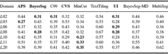
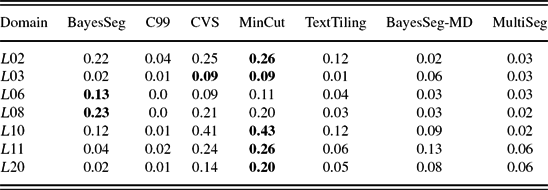
Table 9 presents the WD average scores for each individual domain. The standard deviation values are between 0.09 and 0.27, indicating that some documents are harder to segment than others. The overall results show that single-documents models obtained better results than the multi-document models for all domains. The performance gains range between 0.07 and 0.16 in WD. The best results were spread out across different models, but the most consistent ones overall were MinCut, UI, and BayesSeg. We also report the k BED agreement between automatic segmentation and the human reference (Table 10). Despite not being possible to calculate this metric for all systems,Footnote 8 we can observe that k BED is generally in line with WD as to which segmentors performed better and which are the hardest domains to segment. As before, the standard deviations between 0.01 and 0.39 of k BED also indicates that some documents were harder to segment than others. The k BED metric was much more penalizing than WD, assigning frequently a zero score to many segmentations. The reason for this is that WD just counts segment boundaries in each window. The metric does not take into account that in a given window the boundaries might look very different. In this aspect, k BED is more precise, since it measures the effort of transforming a segmentation into the other.
Average WD scores in MUSED (Remember that BayesSeg-MD and MultiSeg are the multi-document models). Best results are depicted in bold.

Average k BED results in MUSED. Best results are depicted in bold.

Another conclusion from the results is that multi-document models are not able to leverage segmentation on a related set of documents, as single-document models afford better results.
Considering now the reference lectures from Malioutov and Barzilay (Reference Malioutov and Barzilay2006), multi-document models also underperform when compared with single-document models. The best average WD is obtained by MinCut with a 0.42 score, outperforming MultiSeg and BayesSeg-MD results by 0.04 and 0.11, respectively.
4.3 The impact of different media sources
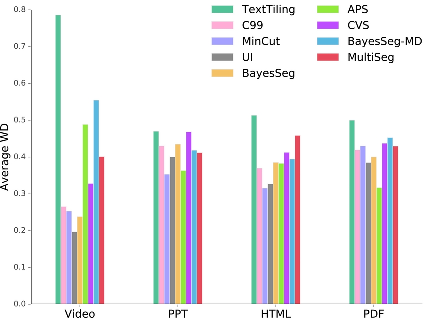
We now analyze the performance of the models considering the different media sources (Figure 6).
Segmentation results grouped by media source.

The results show that even in this scenario multi-document models underperform for all different media sources. Regarding single-document models, the performance varies with the media source of the documents. UI best performs in the video setting, a medium characterized by the low number of segments per document and a high number of words per segment; the fact that APS is designed to model long distant dependencies might explain its performance in PDFs, which is the medium with the highest number of sentences; MinCut performed better in PTT and HTML documents, the media with the lowest number of words. Another observation is that PPT was the hardest medium to segment overall. The explanation is that this media is the one where the textual representations less resemble natural language. PPTs do not offer a coherent discourse structure since they often only have key phrases.
The previous results suggest that since algorithms with distinct characteristics perform differently according to a particular media source, multi-document models might benefit if they incorporate the media source as a feature of the model when segmenting a collection of documents.
4.4 Comparing multi-document models
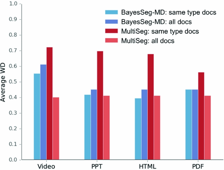
Figure 7 shows the results obtained by multi-document models, when the segmentation of a single document is done with the help of related documents from the same media type (BayesSeg-MD: same type docs and MultiSeg: same type docs), and also when the segmentation of a single document is done with the help of all the remaining related documents (BayesSeg-MD: all docs and MultiSeg: all docs).
Multi-document segmentation models results.

The two multi-document models have opposite behaviors: MultiSeg performs better when all documents are provided (26% overall improvement), and BayesSeg-MD performs better when segmenting documents grouped by type (5% overall improvement). Another difference is that MultiSeg has consistent results across the different sources, whereas BayesSeg-MD is particularly sensitive to video transcript documents.
4.5 Qualitative analysis
In this section, we carry out a qualitative analysis of the results, for both and single and multi-document models, in order to demonstrate the difficulties in segmenting a real dataset of related documents.
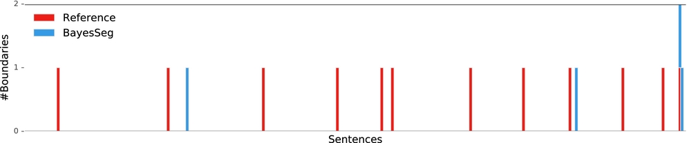
Figure 8 depicts a PPT document segmented by the BayesSeg algorithm. We can observe that most of the boundaries were missed. The difficulty is in detecting the smooth vocabulary changes in the segments. The first two segments describe the concepts of point object and displacement, which have a considerable vocabulary overlap. The cluster of segments before the next boundary placed by BayesSeg shows a similar smooth vocabulary change property. These segments are various topics related to velocity and accelaration. The remaining segments that were merged by BayesSeg describe different aspects of uniform accelerated motion. Finally, the last segment of the document corresponds to the acknowledgments.
BayesSeg segmentation example.

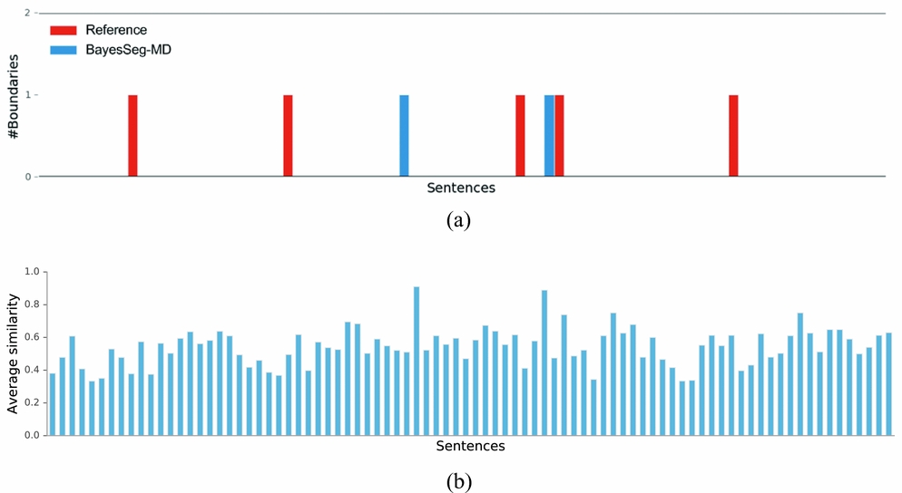
We also analyzed the segmentation of BayesSeg-MD in order to understand its underperformance in MUSED. Two situations might have occurred: (a) the number of segments in the documents is similar to the number of segments in the reference, but segments are not aligned; (b) the number of segments in the documents is very different from the number of segments in the reference (degenerated segmentation). The latter was the main cause of the errors of this model, as there were sixty one documents in which the difference between the number of obtained segments and the number of segments in the reference is higher than 3. An example of such (degenerated) segmentations can be found in Figure 9(a).
Segmentation and sentence similarity example from an HTML document in the L02 domain. (a) example of a degenerated segmentation, (b) average cosine similarity between each sentence of the document and the top-20 most similar sentences in the corresponding domain.

In BayesSeg-MD, similar sentences from related documents are considered when segmenting a target document. The plot in Figure 9(b) shows, for each sentence, the average similarity with the top-20 sentences from other related documents. It can be seen that some sentences have a much higher average similarity than others. This biases the model towards creating segments between such sentences, this is why Figures 9(a) and (b) lineup in the sentences where a spike in average similarity occurs. In other words, sentences that occur frequently throughout the whole collection are likely to be considered as segment boundaries. This was a general pattern of failure, which explains the poor results.
5 Conclusions and future work
We introduced MUSED, a dataset manually segmented by topic, built in order to simulate a real collection of learning materials, gathered from the web. MUSED comprises around twenty documents from different media sources, covering seven subjects in the Physics domains. The average inter-annotator agreement (k BED and WD metrics) is inline with other related works, showing that it is possible for human judges to agree, to some extent, on what is the segmentation of related documents from distinct media sources. The qualitative analysis indicates that the reasons for disagreement are similar to the ones described in previous studies, namely the different perceptions annotators have about the adequate level of granularity for a segment. Despite this, there is a set of prominent segments for which the annotators unanimously agree.
To the best of our knowledge, MUSED is the first dataset that allows a straightforward evaluation of both single- and multiple-documents topic segmentation techniques. The size of MUSED, which is comparable with previous single-document datasets, allows obtaining soundproof regarding multi-document models. Moreover, it is now possible to test multi-document segmentation models in a real-world application scenario, such as segmenting related learning materials from different media sources. All these features were lacking in the previous datasets.
Regarding future work, although single-document models performed better, all annotators felt that seeing related documents helped understanding how to better annotate all the documents. Therefore, we believe in the potential of the multi-document approach. Thus, we would like to develop a better multi-document segmentation model that can effectively leverage repeated topic segment discussions in related documents. Also, we would like to further annotate MUSED with cross-document topic segment relationships, and perform their identification automatically. This will give insights on how the content of a collection of learning materials is structured and how to properly organize it at the topic segment level.