1. Introduction
1.1. Motivation
The bluff-body combustor is prevalent in industrial and aerospace applications, and serves as a canonical burner for many fundamental combustor studies. Fluid dynamics plays an integral role in the operability of bluff-body combustors. For example, the turbulent and coherent structures that stem from hydrodynamic instabilities govern important combustor phenomena such as mixing, entrainment, blowout (Shanbhogue, Husain & Lieuwen Reference Shanbhogue, Husain and Lieuwen2009), and combustion instability (Smith & Zukoski Reference Smith and Zukoski1985; Poinsot et al. Reference Poinsot, Trouve, Veynante, Candel and Esposito1987; Soteriou & Ghoniem Reference Soteriou and Ghoniem1994; O’Connor & Lieuwen Reference O’Connor and Lieuwen2011). Bluff-body combustors are especially prone to combustion instability, which plagues the combustion communities of both the energy and aerospace industries (Zinn & Lieuwen Reference Zinn, Lieuwen, Lieuwen and Yang2005).
Combustion instability is the resonant coupling between the acoustics of the combustor and the unsteady heat release of combustion. This is typically an unwanted phenomenon, which can cause severe damage to hardware, problems with excessive heat transfer, and even blowout of the flame from the combustor. The challenges associated with understanding and predicting combustion instabilities lie in the flame response to the acoustic field. One of the most complicated flame-response mechanisms is the velocity-coupled flame response, where the flame responds dynamically not only to the acoustic velocity, but also to the vortically induced velocity field excited by the acoustics (Lieuwen Reference Lieuwen2012). This vortically induced, or hydrodynamic, velocity field holds critical importance for the flame response but is typically computationally expensive to predict, especially over the broad operability map of the combustor. Local stability analysis applied around a mean flow, which could, for instance, be obtained inexpensively from a Reynolds Averaged Navier Stokes (RANS) solver, offers an inexpensive alternative to traditional computational approaches. With this in mind, this study explores the capability of local stability analysis, applied around a mean flow, to quantify the hydrodynamic stability of bluff-body combustors, and to identify the regions of the flow in which hydrodynamic oscillations are expected to couple most strongly with acoustic oscillations.
1.2. Background
The high-Reynolds-number uniform-density wake behind a bluff body generally exhibits the globally unstable sinuous Von Karman vortex street. This wake instability can be influenced by suction/blowing (Fransson, Konieczny & Alfredsson Reference Fransson, Konieczny and Alfredsson2004), trailing splitter plates (Cardell Reference Cardell1993), wake heating (Roshko Reference Roshko1954; Yu & Monkewitz Reference Yu and Monkewitz1990; Soteriou & Ghoniem Reference Soteriou and Ghoniem1994; Zdravkovich Reference Zdravkovich1997), and numerous other modifications. Strykowski & Sreenivasan (Reference Strykowski and Sreenivasan1990) showed that the oscillations of this global mode can be suppressed by adding a small control cylinder downstream and to one side of the wake. Hill (Reference Hill1992) and Giannetti & Luchini (Reference Giannetti and Luchini2007) identified this region by calculating the direct and adjoint global modes of the steady but unstable flow behind a cylinder at
 $\mathit{Re}\sim 50$
. They overlapped these to obtain the sensitivity of the eigenvalue to changes in intrinsic feedback mechanisms, referred to throughout the paper as the ‘eigenvalue sensitivity’ for reasons of brevity. The eigenvalue sensitivity reveals the region of the flow in which changes to the stability operator, e.g. by passive feedback, cause the biggest eigenvalue drift. This region is known as the wavemaker region of the flow, in that oscillations are generated in this region and the rest of the flow merely responds to these oscillations. This analysis was subsequently refined by Marquet, Sipp & Jacquin (Reference Marquet, Sipp and Jacquin2008) and Luchini, Giannetti & Pralits (Reference Luchini, Giannetti, Pralits, Braza and Hourigan2009) in order to include the influence that the control cylinder has on the base flow. These techniques predict the region in which the control cylinder most stabilizes the flow and identify the corresponding stabilization mechanism.
In this paper, we examine a confined bluff-body wake flow. Lateral confinement can have substantial influences on absolute stability of the wake (Juniper & Candel Reference Juniper and Candel2003). This becomes significant when the confinement ratio,
 $h$
, defined as the width of the outer flow divided by the half-width of the inner flow, is below 4. Confined high-density wakes are particularly absolutely unstable and this effect is strongest when
 $h=1$
(figure 16 of Juniper (Reference Juniper2006)). Rees & Juniper (Reference Rees and Juniper2010) showed that confinement is destabilizing in viscous planar wakes but that the destabilizing influence of confinement starts to diminish below
 $\mathit{Re}=1000$
. In this study we consider the effect of the confining walls, because the confinement ratio is
 $h=0.3$
and the Reynolds number is well above
 $\mathit{Re}=1000$
(ranging from
 $\mathit{Re}=10\,000$
to
 $\mathit{Re}=27\,000$
over the conditions tested).
Bluff-body flame stabilization is used often in aerospace and duct-heating applications. In the reacting wake of a bluff-body-stabilized flame, combustion causes a spatially non-uniform mean-density field with a lower density in the wake. A variety of prior studies has noted fundamental differences in the dynamic character of the flame and flow field at different levels of preheat, and consequently different flame-density ratios (Erickson, Soteriou & Mehta Reference Erickson, Soteriou and Mehta2006; Kiel et al. Reference Kiel, Garwick, Lynch, Gord and Meyer2006; Cross et al. Reference Cross, Fricker, Shcherbik, Lubarsky, Zinn and Lovett2010; Emerson et al. Reference Emerson, O’Connor, Juniper and Lieuwen2012). The first systematic demonstration showing the effects of flame-density ratio in combusting flows was presented by Erickson et al. (Reference Erickson, Soteriou and Mehta2006). Their results show that sinuous vortex shedding is suppressed at high flame-density ratios, but that a large sinuous flow feature gradually grows in prominence as the density ratio across the flame is decreased below values of approximately 2–3. Compared to a uniform-density wake, non-uniform density alters the stability of the flow through the action of baroclinic torque (Lesshafft & Huerre Reference Lesshafft and Huerre2007; Meliga, Sipp & Chomaz Reference Meliga, Sipp and Chomaz2008). Using simple models, Yu & Monkewitz (Reference Yu and Monkewitz1990) expressed the density non-uniformity as a density ratio. They demonstrated the effect of the density-ratio parameter, showing that dense wakes are more absolutely unstable than low-density wakes. Wakes with sufficiently low density relative to the outer flow are globally stable, and only convectively unstable. In this paper we do not rely on the model results in Yu & Monkewitz (Reference Yu and Monkewitz1990), which utilize piecewise-linear velocity/density profiles. Instead, we calculate the absolute growth rate of experimentally measured time-averaged velocity and density profiles. The velocity fields are measured with particle image velocimetry (PIV), and the density fields are estimated from the Mie-scattering images acquired for the PIV measurement. For the moderate density ratios in this study, we find that the flows have a region of absolute instability, even though they are low-density wakes. For these wakes, the sinuous mode is hydrodynamically more globally unstable than the varicose mode, so the sinuous mode dominates when there is no external forcing.
Combustors utilizing reacting bluff-body wakes typically have a streamwise dimension that is longer than their cross-stream dimensions, so the lowest-frequency acoustic mode is longitudinal. A longitudinal acoustic wave forces the bluff-body wake in a varicose manner. Although the bluff-body wake is more hydrodynamically unstable to sinuous motions, it is also convectively unstable to varicose motions. It amplifies these and causes heat-release oscillations in time with the acoustic oscillations. If these heat-release oscillations are sufficiently in phase with the pressure oscillations, then these thermoacoustic oscillations become self-sustained. Experiments show that the varicose mode seems to be especially troublesome for thermoacoustic oscillations (Emerson, Murphy & Lieuwen Reference Emerson, Murphy and Lieuwen2013). The local analysis used in this study can find the direct and adjoint global modes for the varicose motion in the same way as they can for the sinuous motion, even when the flow is not globally unstable. This is difficult with global analyses, which are strongly influenced by the downstream boundary condition when the flow is not globally unstable (Garnaud et al. Reference Garnaud, Lesshafft, Schmid and Huerre2013).
The above studies demonstrate that low-density-ratio reacting bluff-body wakes oscillate sinuously in the absence of acoustic forcing or thermoacoustic oscillations. Experimental studies on low-Reynolds-number uniform-density wakes show that these oscillations are driven by a wavemaker region just behind the bluff body. The goal of this paper is to answer three questions. The first question is whether or not local stability analysis is an appropriate tool for studying the hydrodynamics of high-
 $\mathit{Re}$
low-density wakes. The second question is whether we can use direct/adjoint techniques to identify the wavemaker region of our experimentally measured reacting bluff-body wake in the sinuous and varicose regimes. The third question is what influences, if any, do the lip velocity and density ratio have on the wavemaker and the region of high receptivity to velocity forcing.
2. Local hydrodynamic stability analysis
The goals outlined at the end of § 1 are accomplished by performing a local stability analysis around an experimentally derived time-averaged base flow at high Reynolds number. It is important to note that this analysis is local-only, and that the global modes presented in this paper are estimated by combining the local results. The procedure for combining the local results is outlined later in this section. The use of a base flow that is time averaged, rather than a steady solution to the Navier–Stokes equations, will be discussed in § 5.
A local stability analysis has two advantages over a 2D global stability analysis. Firstly, the streamwise domain of the experimental data is shorter than the length of the direct global mode. It is significantly shorter than that in figure 19 of Giannetti & Luchini (Reference Giannetti and Luchini2007), which shows the influence of the downstream boundary. This presents a challenge for a 2D global stability analysis because the boundaries lie in regions in which the direct and adjoint global modes have significant amplitude. This means that boundary conditions at the upstream and downstream ends of the domain need to be carefully chosen. This is a challenge that faces the global analysis approach, although it is not an insurmountable problem. On the other hand, in a local analysis, slices of the flow at each streamwise location are considered independently, which means that no streamwise boundary conditions need to be imposed. The removal of upstream and downstream boundary conditions is a convenience of the local analysis compared to a global scheme. Secondly, 2D global stability analysis is much more computationally expensive than a local analysis. For these reasons, we use a local stability analysis, as in Juniper & Pier (Reference Juniper and Pier2015), to reconstruct the direct and adjoint global modes.
In a local analysis, the wavelength of the perturbations is assumed to be much shorter than the length scale over which the base flow varies (the WKBJ approximation). This approximation is valid for flows that are nearly parallel, but it also works surprisingly well for flows that are significantly non-parallel (Pier Reference Pier2008). The motivations for using the WKBJ approximation parallel those for using a local analysis, discussed in the previous paragraph. The justification for using this approach is that it is robust for weakly non-parallel flows like those considered in this analysis. Additionally, as opposed to a fully global approach, this approach also precludes acoustic feedback, which is a benefit for isolating hydrodynamic instabilities.
The governing equations are Navier–Stokes equations, linearized around a parallel base flow that is symmetric about the flow centreline. Equations (2.1)–(2.3) show the governing equations, where
 $x$
and
 $y$
are the streamwise and transverse directions, and
 $U_{0}$
and
 ${\it\rho}_{0}$
are the base axial velocity and density. Also,
 $u$
,
 $v$
, and
 $p$
are the transverse dependence of the linear perturbations to the axial velocity, transverse velocity, and pressure, which take the general form
 $p(y)\text{e}^{-\text{i}{\it\omega}t}\text{e}^{\text{i}kx}$
(for the pressure, for example).
 $$\begin{eqnarray}\text{i}ku(y)+\frac{\text{d}v}{\text{d}y}=0,\end{eqnarray}$$
 $$\begin{eqnarray}\displaystyle -\text{i}{\it\omega}{\it\rho}_{0}(y)u(y)+\text{i}kU_{0}(y){\it\rho}_{0}(y)u(y)+{\it\rho}_{0}(y)\frac{\text{d}U_{0}}{\text{d}y}v(y)=-\text{i}kp(y)+\frac{1}{\mathit{Re}}\!\left(\!-k^{2}u(y)+\frac{\text{d}^{2}u}{\text{d}y^{2}}\!\right)\!, & & \displaystyle \nonumber\\ \displaystyle & & \displaystyle\end{eqnarray}$$
 $$\begin{eqnarray}-\text{i}{\it\omega}{\it\rho}_{0}(y)v(y)+\text{i}kU_{0}(y){\it\rho}_{0}(y)v(y)=-\frac{\text{d}p}{\text{d}y}+\frac{1}{\mathit{Re}}\left(-k^{2}v(y)+\frac{\text{d}^{2}v}{\text{d}y^{2}}\right).\end{eqnarray}$$
The base flow includes the spatially varying base-density field. This approach captures instabilities generated by the Kelvin–Helmholtz mechanism, which is influenced by the base-density non-uniformity, although it does not capture the Darrieus–Landau instability, the inclusion of which is left to future work. The boundary conditions are no slip and impermeability at the confining wall, and sinuous or varicose modes at the flow centreline. A Fourier/Laplace decomposition is performed in time and in the
 $x$
-direction such that the governing equations reduce to an eigenvalue problem that is only satisfied for certain eigenvalue pairs of the streamwise wavenumber,
 $k$
, and the angular frequency,
 ${\it\omega}$
(Huerre & Monkewitz Reference Huerre and Monkewitz1990, Reference Huerre, Monkewitz, Batchelor, Moffat and Worster2000). The stages of the local analysis are described in detail in Juniper, Tammisola & Lundell (Reference Juniper, Tammisola and Lundell2011), and are summarized next.
Stage 1 of the local analysis is to evaluate the absolute growth rate,
 ${\it\omega}_{0}$
, as a function of downstream distance,
 $x$
. The absolute growth rate is the temporal growth rate of waves with zero group velocity at that streamwise location. These waves satisfy
 $\text{d}{\it\omega}/\text{d}k=0$
. Stage 2 of the local analysis is to evaluate the linear global mode frequency,
 ${\it\omega}_{g}$
, and the wavemaker location. Stage 3 of the local analysis is to force the flow at
 ${\it\omega}_{g}$
and to evaluate the spatial growth rates of the downstream-travelling wave,
 $k^{+}$
, and the upstream-travelling wave,
 $k^{-}$
. These can then be combined to form the direct global mode and the adjoint global mode (Juniper et al.
Reference Juniper, Tammisola and Lundell2011; Juniper & Pier Reference Juniper and Pier2015). In this analysis, we do not develop non-parallelism, and we do not solve an equation for the slowly varying amplitude.
Stages 1–3 of the analysis proceed as follows. In stage 1, the local stability analysis is performed with the software package InstaFlow, described in Juniper et al. (Reference Juniper, Tammisola and Lundell2011) and Juniper (Reference Juniper2012). At each streamwise location, the time-averaged streamwise velocity,
 $U(y)$
, and time-averaged density,
 ${\it\rho}(y)$
, are projected onto Gauss–Lobatto-spaced points in the cross-stream,
 $y$
, direction. The Gauss–Lobatto grid consists of 60 grid points spanning half of the channel from the centreline to the wall. A grid independence study showed that this grid provided better than 0.12 % error in the eigenvalue. The governing equations and boundary conditions are expressed in matrix form using Chebyshev differentiation matrices. At each slice, this generates a matrix eigenvalue problem for
 ${\it\omega}$
in terms of
 $k$
. Saddle points of
 ${\it\omega}(k)$
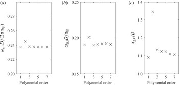
are found and their Briggs–Bers validity is checked. These saddle points are then tracked as the streamwise location changes. For these flows, there is usually only one valid saddle point for sinuous oscillations and another valid saddle point for varicose oscillations. In stage 2, the linear global mode frequency is calculated by fitting a seventh-order Padé polynomial to
 ${\it\omega}_{0}(x)$
and finding the saddle position in the complex
 $(X,{\it\omega}_{0})$
-plane (Juniper & Pier Reference Juniper and Pier2015), denoted (
 $x_{g}$
,
 ${\it\omega}_{g}$
). The dependence of
 $x_{g}$
and
 $w_{g}$
on the polynomial order is shown in figure 1. In stage 3 of the analysis, each of the local analyses (at each axial position) is repeated, this time solving for
 $k$
when
 ${\it\omega}={\it\omega}_{g}$
. For a given value of
 ${\it\omega}$
, there are two valid solutions to
 $k$
, which are the
 $k^{+}$
and
 $k^{-}$
spatial branches. These
 $k^{+}$
and
 $k^{-}$
branches are conveniently identified at
 $x_{g}$
, where they are singular. The
 $k^{+}$
branch is the more spatially amplified branch when moving in the downstream direction, and is numerically tracked while walking downstream from
 $x_{g}$
, while the
 $k^{-}$
branch is the more spatially amplified branch when moving in the upstream direction, and is numerically tracked while walking upstream of
 $x_{g}$
. At each stage, the eigenfunctions are normalized to have
 $u^{2}+v^{2}+p^{2}=1$
.
Dependence of
 ${\it\omega}_{g}$
and
 $x_{g}$
on the Padé polynomial order, showing (a) real part of
 ${\it\omega}_{g}$
non-dimensionalized as the Strouhal number, (b) imaginary part of
 ${\it\omega}_{g}$
, and (c)
 $x_{g,r}$
, shown for a representative case (
 ${\it\rho}_{u}/{\it\rho}_{b}=1.7$
,
 $U_{lip}=30$
m s
 $^{-1}$
).

3. Design of experiments
The goal of the experiments is to obtain estimates of base flows for stability analysis, and to measure the corresponding global mode frequencies and mode shapes. The facility and its instrumentation are described in detail in the next subsection. Its test section is a nominally two-dimensional bluff-body combustor with premixed inflow; therefore, the base flow is a planar wake with spatially varying density, confined within a channel. Three different streams are premixed upstream of the test section: room-temperature natural gas, room-temperature air, and a vitiated stream. The vitiated stream consists of hot combustion products from a natural-gas preburner. Independent control of these three streams provides significant flexibility of the flame-density ratio and the bluff-body lip velocity in the test section. This is significant, because the flame-density ratio controls the global mode growth rate,
 ${\it\omega}_{g,i}$
, and the lip velocity governs the global mode frequency,
 ${\it\omega}_{g,r}$
, in the linear analysis. The test matrix, discussed in § 3.3, is constructed to vary these parameters.
3.1. Experimental facility
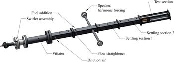
The experimental rig, shown in figures 2 and 3, consists of two premixed methane–air combustors in series. The first combustor is used to vitiate the flow and raise its temperature. The second, bluff-body-stabilized combustor, consists of a rectangular section with a bluff body spanning the width of the combustor, creating a nominally 2D flow. The bluff body has a diameter of
 $D=19.1$
mm. The aspect ratio of bluff-body height to chamber width is 0.15. This combustor has quartz windows for optical access from all four sides. The bluff body used in the test section, shown in figure 3(b), has a 2D ballistic shape. Additional fuel- and air-injection sources are located between the two burners, allowing substantial flexibility in density ratio and lip velocity. The Reynolds number for these experiments varies from
 $\mathit{Re}=10\,000$
to
 $\mathit{Re}=27\,000$
. Further details of this facility and its design are provided in Emerson et al. (Reference Emerson, O’Connor, Juniper and Lieuwen2012).
Schematic of the atmospheric-pressure vitiated bluff-body rig.
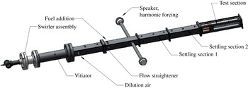
Drawings of (a) the test section and (b) the bluff body.

3.2. Diagnostics
Velocity fields are measured using particle-image velocimetry (PIV). Mie-scattering images for high-speed PIV are obtained as follows. The flow is seeded with 5
 ${\rm\mu}$
m
 $\text{Al}_{2}\text{O}_{3}$
particles, chosen due to their durability in reacting flows and their high refractive index (Melling Reference Melling1997). This particle size is chosen because it is large enough to slow down accumulation on and clouding of the test-section windows, while retaining a sufficiently small Stokes number to accurately track the flow at the frequencies of interest. Following the work by Mei (Reference Mei1996), the Stokes number calculated for this flow and seed-particle combination is 0.015. This Stokes number is calculated using a kinematic viscosity of
 $3\times 10^{-4}~\text{ m}^{2}~\text{s}^{-1}$
and an oscillation frequency of 850 Hz (roughly the highest global mode frequency encountered). This Stokes number is comfortably below the cutoff Stokes number for solid particles in air (Mei Reference Mei1996), which is in the range of 0.02–0.04 and would correspond to a frequency of at least 1500 Hz.
The particle-laden flow is illuminated with a double-pulsed Nd:YLF laser, with wavelength of 527 nm, pulse duration of 100 ns, and 4 mJ/pulse pulse energy. Each of the two lasers in the double-pulsed system is operated at 5000 Hz. The laser beams are expanded with a
 $-$
50 mm cylindrical lens into an expanding sheet, and the sheet is shaped with a 750 mm cylindrical lens to have a nominally 4 mm thickness. An expanding sheet is chosen instead of a collimated sheet because of the large test area. The time delay,
 $\text{d}t$
, between the two illuminating laser pulses of a given pair was
 $12~{\rm\mu}\text{s}$
. The short
 $\text{d}t$
is responsible for much of the velocity uncertainty, as discussed below. Mie scattering image pairs are captured by a high-speed CMOS camera with
 $20~{\rm\mu}\text{m}$
pixels. The camera is outfitted with a 55 mm lens, with aperture at
 $f/5.6$
. The camera is operated with a pixel resolution of
 $640\times 448$
, with image pairs acquired at a frame rate of 5 kHz. The optical configuration produces a magnification of 1:12.5, such that the measurement domain covers a
 $640\times 320$
pixel region of the CMOS chip, which corresponds to a region of the combustor that is roughly 160 mm long in the axial direction and 80 mm wide in the transverse direction. The measurement plane is located at the centre span of the bluff body. The diffraction-limited spot size for this configuration is
 $7~{\rm\mu}\text{m}$
. Slight defocusing, together with the natural aberration and imperfections of the imaging optics, distributes the scattered light from the particles over a nominal three-pixel diameter. A bandpass optical filter is placed in front of the camera in order to reject the majority of flame and other background luminosity. The filter pass band is centred at 527 nm and has a transmission of greater than 93 % from 517 to 537 nm.
Velocity vectors are computed from the Mie-scattering image pairs using a digital cross-correlation algorithm (Willert Reference Willert1991) with a multi-pass approach (Soria Reference Soria1996) and 2D Gaussian subpixel interpolation (Willert Reference Willert1991). The multi-pass analysis consists of a single pass with
 $64\times 64$
pixel interrogation windows and 50 % overlap between the interrogation windows, followed by two passes with
 $32\times 32$
pixel interrogation windows and 50 % overlap between the interrogation windows. The spacing between vectors is 4 mm.
Post-processing algorithms are used to discard and replace a small number of spurious vectors, and to validate the PIV data. First, any velocity vector with an axial component outside of a
 $20\pm 90~\text{m}~\text{s}^{-1}$
range or a transverse component outside of a
 $\pm$
45 m s
 $^{-1}$
range is discarded. These ranges are based on the expected range of mean axial and transverse velocities and, additionally, they conservatively accommodate coherent structures with unsteady velocity on the order of the nominal 50 m s
 $^{-1}$
lip velocity. Next, any velocity vector whose velocimetry calculation has a peak correlation coefficient of less than 0.2 is discarded and a local validation method discards neighbouring vectors whose ratio of difference to average velocity magnitude is greater than 20 % of the r.m.s. of the nearest neighbours. This threshold is consistent with values recommended in the literature (Nogueria, Lecuona & Rodriguez Reference Nogueria, Lecuona and Rodriguez1997). In all, less than 1 % of the total velocity vectors are discarded and their values filled with the instantaneous average of neighbouring vectors.
The PIV measurement is calibrated by imaging a black anodized aluminium calibration plate with a laser-etched pattern, which is located coincidently with the laser-light sheet. The laser-etched pattern consists of a regularly spaced grid of crosses, composed of 0.3 mm thick lines, with spacing of 6 mm and with positional uncertainty of 0.004 %. The spatial coordinates of the Mie-scattering images and resultant velocity fields are mapped to this grid. The worst-case calibration error is estimated to be one pixel over the large 160 mm calibration plate, which would result in a small 0.2 % bias error. The phase jitter between the pair of laser-illumination pulses is measured to be on the order of nanoseconds, which is significantly less than the relatively long 100 ns duration at half-maximum of each illumination. Therefore, the duration of the laser illumination dominates the temporal measurement uncertainty, which is less than 1 % of the time delay between the pair of illumination pulses. Peak locking during subpixel interpolation (Fincham & Spedding Reference Fincham and Spedding1997), combined with the relatively short
 $\text{d}t$
, is estimated to provide a velocity uncertainty of 4 %. In- and out-of-plane motion dominates the random velocity uncertainty over much of the measurement domain, and increases with distance from the measurement centre (located at
 $x/D=4$
). For example, at axial positions 20 mm from the measurement centre (i.e. at
 $x/D=3$
and
 $x/D=5$
), this uncertainty is 5 %. As the measurement position moves to the extreme axial extents of the measurement, i.e. to
 $x/D=0$
and
 $x/D=8$
, this uncertainty increases linearly to 20 %. However, this uncertainty due to in- and out-of-plane motion applies to turbulence and secondary instabilities in this flow, but does not directly impact the nominally 2D hydrodynamic motion and time-averaged velocity field of interest. Just downstream of the bluff body, from
 $x/D=0$
to
 $x/D=0.3$
, laser-light scattering off of the bluff body spoils the PIV measurement and introduces large uncertainties; we do not report results from this region.
The measured oscillatory velocity magnitude is subject to an additional source of uncertainty. Following the seeding particle Stokes number discussion above, the seeding particles are expected to respond at the forcing frequency with 92 % of the flow-response amplitude, and with less than a 20° phase delay. It is important to note that the significant experimental velocity field uncertainties lie in the unsteady-velocity magnitude. The uncertainty in the measured oscillatory velocity affects the validation of the stability analysis, and is quantified with error bars when compared to stability analysis predictions. The time-averaged velocity, which is used as an input to the stability analysis, is not subject to these larger experimental uncertainties.
The time-averaged density field is estimated from the Mie-scattering images. An edge-detection algorithm is used to extract the sharp jump in seed-particle density that occurs at the flame sheet (Gülder et al. Reference Gülder, Smallwood, Wong, Snelling, Smith, Deschamps and Sautet2000). The instantaneous density is then specified as a binary field having either the burned or the unburned value. The unburned-density value is estimated from a temperature measurement just upstream of the test section, and a gas composition consisting of the vitiated gas stream mixed with the fresh air and fuel streams. The burned-density value is estimated as the adiabatic flame temperature of this mixture. The instantaneous density fields are then averaged at each location to obtain the temporally averaged density field. The key assumption behind this method is that the density change occurs across a thin unbroken reaction zone, such that there is minimal turbulent mixing between reactants and products outside of this thin zone. This assumption is supported by the modified Borghi–Peters diagram (Peters Reference Peters1999), due to two considerations for this flow. The first consideration is that the laminar flame thickness is very thin relative to the bluff-body diameter, which is well satisfied for this problem, as verified by detailed chemical kinetic calculations of an unstretched premixed flame (using GRI 3.0), showing that the estimated flame thickness is roughly 2 % of the bluff-body diameter (and hence the integral length scale). The second consideration is that the turbulence intensity is less than 50 times the laminar flame speed. We quantified the uncertainty of this density-ratio measure in a previous study, and demonstrated that it is better than 10 % (Emerson Reference Emerson2013), which is less than the step changes in density ratio reported here during density-ratio sweeps.
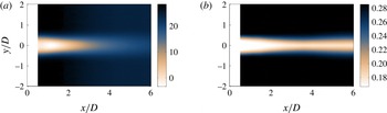
Contour plots of the measured base flow, showing (a) axial velocity field and (b) density field. Conditions are
 ${\it\rho}_{u}/{\it\rho}_{b}=1.7$
,
 $U_{lip}=30$
m s
 $^{-1}$
, which are qualitatively representative of all cases.

3.3. Test-matrix design
The test matrix is designed to vary the global mode growth rate and frequency. This is accomplished by sweeping two stability parameters: the density ratio and the lip velocity. Previous studies have shown that the absolute growth rate is sensitive to the density ratio (Yu & Monkewitz Reference Yu and Monkewitz1990), and that the global mode frequency scales with the bluff-body lip velocity,
 $f_{g}=St_{D}U_{lip}/D$
(Prasad & Williamson Reference Prasad and Williamson1997). In these experiments, the density ratio is varied over the range of
 ${\it\rho}_{u}/{\it\rho}_{b}=1.7$
to
 ${\it\rho}_{u}/{\it\rho}_{b}=2.5$
to sweep the global mode growth rate. For each density ratio, the bluff-body lip velocity is varied from 20 to 70 m s
 $^{-1}$
in order to vary the global mode frequency. The Reynolds number for these experiments ranges from
 $\mathit{Re}=10\,000$
to 27 000.
The experimental parameters, bluff-body lip velocity
 $U_{lip}$
and density ratio
 ${\it\rho}_{u}/{\it\rho}_{b}$
, are determined as follows. The bluff-body lip velocity is calculated as
 $U_{lip}=\dot{m}/({\it\rho}_{u}A_{lip})$
, which is an average streamwise flow velocity. The mass-flow rate,
 ${\dot{m}}$
, is the mass-flow rate entering the test section. The area,
 $A_{lip}$
, is the cross-sectional area of the flow at the plane of the bluff-body trailing edge, accounting for the blockage of the bluff body. The density of the wake, which consists of burned products, is denoted
 ${\it\rho}_{b}$
, and the density of the unburned flow outside of the wake is denoted
 ${\it\rho}_{u}$
. The values of these densities are estimated according to the procedure outlined at the end of § 3.2.
4. Experimental results
4.1. Base-flow approximation
This section describes the experimentally measured mean-flow field, which is the base flow used for the stability analysis. The time-averaged axial velocity field is plotted in figure 4(a). This plot shows that the velocity profile is that of a recirculating wake. The reverse flow in the recirculation zone reaches a maximum reverse-flow velocity between one and two bluff-body diameters downstream, which is generally true for all conditions tested in this study. Figure 4(b) plots the time-averaged density field generated by the bluff-body-stabilized flame. This plot shows that the mean-density field consists of a region of low-density flow (hot combustion products) in the wake region and high-density flow (reactants) in the free stream. The density field also illustrates that this flow holds a nearly flat flame, which ‘pinches’ slightly just downstream of the recirculation zone. The small spreading angle of the flame is due to the fact that the free-stream velocity is two orders of magnitude faster than the laminar flame speed.
4.2. Flow dynamics
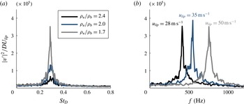
Figure 5 shows power spectra of the unsteady transverse velocity at three different density ratios and velocities. Figure 5(a) presents power spectra for three values of
 ${\it\rho}_{u}/{\it\rho}_{b}$
, and shows that there is a strong narrowband peak at
 $St_{D}=0.24$
. The frequency of this response is proportional to the bluff-body lip velocity, as is evident in figure 5(b). This indicates that the strong oscillation is driven by a hydrodynamic mechanism, not an acoustic mechanism.
Power spectra of the centreline transverse velocity at
 $x/D=5$
,
 $y/D=0$
, for (a) three density ratios at
 $U_{lip}=50$
m s
 $^{-1}$
and (b) three velocities at
 ${\it\rho}_{u}/{\it\rho}_{b}=1.7$
.

The global mode associated with the
 $St_{D}=0.24$
oscillations is sinuous, as it is for a non-reacting wake. To illustrate this, we performed a proper orthogonal decomposition (POD) on the velocity field (Berkooz, Holmes & Lumley Reference Berkooz, Holmes and Lumley1993). The POD decomposes the velocity field,
 $\boldsymbol{u}(\boldsymbol{x},t)$
, into a series of
 $N$
spatial basis functions,
 ${\it\phi}_{n}(\boldsymbol{x})$
, each with temporal evolution of
 $q_{n}(t)$
, such that
 $$\begin{eqnarray}\boldsymbol{u}(\boldsymbol{x},t)=\mathop{\sum }_{n=1}^{N}q_{n}(t){\it\phi}_{n}(\boldsymbol{x}).\end{eqnarray}$$
Here,
 $\boldsymbol{x}$
is a spatial position vector that points to the axial position,
 $x$
, and transverse position,
 $y$
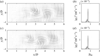
. Figure 6 shows the most energetic pair of POD modes along with the corresponding spectra of their time coefficients. This pair of POD modes is selected because the two modes combine to reconstruct the global mode (Ma, Karamanos & Karniadakis Reference Ma, Karamanos and Karniadakis2000; Konstantinidis, Balabani & Yianneskis Reference Konstantinidis, Balabani and Yianneskis2007; Perrin et al.
Reference Perrin, Braza, Cid, Cazin, Barthet, Sevrain, Mockett and Thiele2007). The time coefficients for each POD mode are denoted
 $q_{n}$
and their power spectral densities are denoted
 $|q_{n}|^{2}$
, where
 $n$
is the number of the POD mode. Together, these two modes represent a strong sinuous vortex shedding at the
 $St_{D}=0.24$
frequency. A detailed discussion of the dynamics of this flow is provided by Emerson et al. (Reference Emerson, O’Connor, Juniper and Lieuwen2012) and Emerson (Reference Emerson2013).
Most energetic pair of POD modes consisting of modes 1 and 2, for
 ${\it\rho}_{u}/{\it\rho}_{b}=1.7$
and
 $U_{lip}=30$
m s
 $^{-1}$
. Spatial modes are illustrated in (a,c) with velocity-vector fields. Power spectral densities of the corresponding time-dependent POD coefficients for modes 1 and 2,
 $|q_{1}|^{2}$
and
 $|q_{2}|^{2}$
, are shown in (b,d).

5. Computational results and comparison
In this section, the predictions from the local stability analysis, applied around the mean flow, are compared with the flow dynamics measured experimentally. The validity of applying linear stability analysis to turbulent mean flows is still an area of active research. On the one hand, Reynolds & Hussain (Reference Reynolds and Hussain1972) provided a theoretical basis by dividing the flow into a mean component, a periodic component, and a turbulent component. By considering a local stability analysis of a turbulent shear layer, they concluded that a turbulence model needs to be included in the stability analysis. On the other hand, other studies have obtained accurate results without using turbulence models. For example, Meliga, Pujals & Serre (Reference Meliga, Pujals and Serre2012) performed a linear stability analysis on the mean flow around a D-shaped cylinder at
 $\mathit{Re}=13\,000$
, using a frozen eddy viscosity approach. Their predicted frequency was reasonably close to that of their oscillating flow (
 ${\it\omega}=1.57$
, giving
 $St=0.25$
). Mettot, Sipp & Bezard (Reference Mettot, Sipp and Bezard2014) performed a similar study on the same D-shaped cylinder but with molecular viscosity instead of a frozen eddy viscosity. Their predicted frequency was close to that of Meliga et al. (Reference Meliga, Pujals and Serre2012) and their predicted growth rate was also positive (
 ${\it\sigma}=0.26$
). Given the success of Mettot et al. (Reference Mettot, Sipp and Bezard2014) at predicting frequency and spatial structure without turbulence models in a configuration close to ours, we also use only molecular viscosity in our stability analysis. It is interesting to note that Barkley (Reference Barkley2006) also performed a stability analysis around the mean flow behind a cylinder at
 $Re=45$
–180. Like Meliga et al. (Reference Meliga, Pujals and Serre2012), Barkley found that this produces an eigenmode with the same frequency as the original oscillating flow, but with zero growth rate. In this case, however, turbulent models would not be appropriate because the flow, although oscillating, was laminar.
The main focus of the studies by Meliga et al. (Reference Meliga, Pujals and Serre2012) and Mettot et al. (Reference Mettot, Sipp and Bezard2014) was to perform sensitivity analysis of the flow by combining the direct and adjoint eigenfunctions of the most unstable eigenmodes. They were not as concerned with the growth rate. In this section, we start by computing the linear global mode frequency, growth rate, and mode shapes around the time-averaged experimental data and then comparing the results with the full experimental data. This reveals whether the stability analysis can predict the correct frequency and mode shape, which is a prerequisite for finding the eigenvalue sensitivity, discussed in § 5.2. During this process, we also examine the growth rate, because we find the same relationship between (i) the linear global mode growth rate and (ii) the nonlinear limit-cycle amplitude that is expected for laminar flows near a Hopf bifurcation.
5.1. Local stability analysis
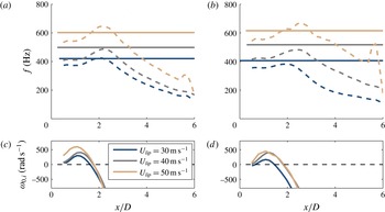
Figure 7(a,b) compare the streamwise dependence of the absolute frequency,
 ${\it\omega}_{0,r}/2{\rm\pi}$
(dashed lines), with the measured global mode frequency (solid lines). Figure 7(c,d) plot the absolute growth rate,
 ${\it\omega}_{0,i}$
, and reveals a pocket of absolute instability around
 $0.2<x/D<2$
. The stability analysis correctly captures that higher bluff-body lip velocities lead to higher frequencies.
(a,b) Comparison of the measured global mode frequency (solid lines) and the predicted absolute frequency (dashed lines). (c,d) For reference, the absolute growth rate is shown. (a,c) are for a fixed density ratio of
 ${\it\rho}_{u}/{\it\rho}_{b}=1.7$
and (b,d) are for a fixed density ratio of
 ${\it\rho}_{u}/{\it\rho}_{b}=2.0$
.

The linear global mode frequency and growth rate,
 $f_{g,l}$
and
 ${\it\omega}_{g}$
, are calculated by finding the saddle point of
 ${\it\omega}_{0}$
in the complex
 $X$
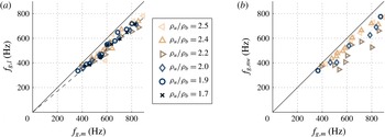
-plane, as described in § 2. Figure 8(a) compares the predicted global mode frequency,
 $f_{g,l}$
, with the experimentally measured frequency,
 $f_{g,m}$
. These are compared for various values of the lip velocity at six different density ratios. This comparison shows that the local linear analysis consistently underpredicts the frequency by around 15 %, across all density and velocity ratios. This can be compared with the global linear analysis of Barkley (Reference Barkley2006), which slightly underpredicts the frequency and the global linear analyses of Meliga et al. (Reference Meliga, Pujals and Serre2012), Mettot et al. (Reference Mettot, Sipp and Bezard2014), which overpredict the frequency by around 10 %. Regarding local analyses, the same 10–15 % underprediction of the frequency was seen in a local analysis by Juniper et al. (Reference Juniper, Tammisola and Lundell2011) for a uniform-density wake flow in a channel at
 $\mathit{Re}=100$
. Similarly, a smaller underprediction was seen by Giannetti & Luchini (Reference Giannetti and Luchini2007) for the local analysis of the flow around a cylinder, but only for Reynolds numbers greater than 80. Interestingly, the degree of accuracy in the frequency is similar to that of previous studies based on analyses around the mean flow, but for studies that determined the base flow with RANS simulations rather than experiments.
Another way to estimate the global mode frequency from the local analysis is to use the frequency-selection criterion from the nonlinear wave-front theory of Pier & Huerre (Reference Pier and Huerre1996). The nonlinear wave-front theory predicts that the experimentally measured frequency and spatial growth rate should match those predicted by the local analysis at the streamwise position where the flow transitions from convective to absolute instability. Therefore, the global mode frequency can be estimated from the absolute frequency,
 ${\it\omega}_{0,r}$
, at the upstream point of
 ${\it\omega}_{0,i}=0$
. Figure 8(b) compares the frequency predicted from the nonlinear wavefront theory,
 $f_{g,nw}$
, to the experimentally measured frequency. The figure shows a slight underprediction of the global mode frequency similar to that observed from the saddle-point approach.
Comparison of measured and predicted global mode frequencies, from velocity sweeps at six different density ratios. (a) Compares measured global mode frequencies,
 $f_{g,m}$
, to those predicted from the saddle point of the
 ${\it\omega}_{0}(X)$
approach,
 $f_{g,l}$
. Solid line corresponds to
 $f_{g,l}=f_{g,m}$
. Dashed line is least-squares fit to the slope of
 $f_{g,l}$
versus
 $f_{g,m}$
. (b) Compares measured global mode frequencies to those predicted from nonlinear wave-front theory,
 $f_{g,nw}$
. Cases where the PIV measurement was noisy near the transition point from convective to absolute instability were omitted from (b).

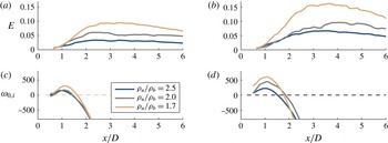
Axial dependence of the oscillatory kinetic energy,
 $E$
(a,b), and predicted absolute growth rate (c,d). Results are shown for density-ratio sweeps at fixed velocities of
 $U_{lip}=30$
m s
 $^{-1}$
(a,c) and
 $U_{lip}=50$
m s
 $^{-1}$
(b,d). As expected, the amplitude of the mode grows most rapidly in the region of strong absolute instability.

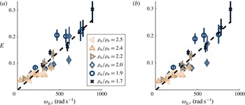
Maximum of the oscillatory kinetic energy,
 $E(x)$
, plotted as a function of the linear global mode growth rate. This is shown for a combination of five values of
 $U_{lip}$
and six values of
 ${\it\rho}_{u}/{\it\rho}_{b}$
and for
 $\max (E)$
(a) and for
 $E(x/D=3.0)$
(b). The dashed line is a linear least-squares fit. The error bars represent PIV measurement uncertainty due to the Stokes number considerations discussed in § 3.2.

Next, we define the local energy of the oscillations,
 $E(x)$
, by integrating the spectral energy of the measured streamwise and cross-stream velocity components from
 $St_{D}=0.20$
to
 $St_{D}=0.28$
, and then integrating this across the transverse dimension,
 $y$
, from the flow centreline to the channel wall:
 $$\begin{eqnarray}E(x)=\int _{y}\int _{0.20}^{0.28}(|u(x,y,St_{D})|^{2}+|v(x,y,St_{D})|^{2})\,\text{d}St_{D}\,\text{d}y.\end{eqnarray}$$
Figure 9 compares
 $E(x)$
(a,b) with the local absolute growth rate
 ${\it\omega}_{0,i}$
(c,d) at two values of
 $U_{lip}$
. The energy of the oscillations grows rapidly in the absolutely unstable region. Therefore, we hypothesize that the oscillations at the global mode frequency are generated by hydrodynamic feedback mechanisms in the absolutely unstable region. Furthermore, the oscillations’ energy increases as the linear global mode growth rate increases. This relationship can be examined more precisely by assuming that the complex amplitude,
 $A$
, of the oscillations can be modelled by the Stuart–Landau equation (Landau Reference Landau1944; Stuart Reference Stuart1958; Provansal, Mathis & Boyer Reference Provansal, Mathis and Boyer1987):
 $\text{d}A/\text{d}t={\it\omega}_{g,i}A-{\it\beta}|A|^{2}A$
. This is a good approximation when the operating point is close to that of the onset of oscillations, which is not always the case here. Saturation is achieved when
 $\text{d}A/\text{d}t=0$
, which leads to the relation that
 $|A|^{2}\propto {\it\omega}_{g,i}$
, where
 $A^{2}\propto E$
, as defined above. Figure 10 plots the maximum of
 $E$
against
 ${\it\omega}_{g,i}$
(calculated from the local linear analysis) for five values of
 $U_{lip}$
and three values of
 ${\it\rho}_{u}/{\it\rho}_{b}$
. The fact that
 $E$
is proportional to
 ${\it\omega}_{g,i}$
shows that the linear growth rate, which is calculated here around the turbulent mean flow, has the same relationship to the nonlinear saturated amplitude as that which would be expected for a laminar base flow. This is a surprising result, especially given that the growth rates calculated from global analyses by Barkley (Reference Barkley2006), Meliga et al. (Reference Meliga, Pujals and Serre2012), Mettot et al. (Reference Mettot, Sipp and Bezard2014) do not have this characteristic.
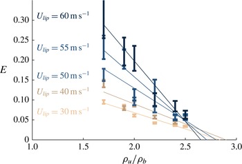
Maximum of the oscillatory kinetic energy,
 $E(x)$
, plotted as a function of the density ratio, shown for a combination of five values of
 $U_{lip}$
and six values of
 ${\it\rho}_{u}/{\it\rho}_{b}$
. Linear least-squares-fit lines are overlaid for each velocity. The error bars represent PIV measurement uncertainty due to the Stokes number considerations discussed in § 3.2.

Figures 9 and 10 also show that the stability analysis correctly captures the role of the density ratio: lower density ratios lead to higher absolute growth rates and larger limit-cycle amplitudes in this flow. The density ratio at which the flow becomes unstable,
 ${\it\rho}_{u}/{\it\rho}_{b}|_{crit}$
, can be calculated from this data by extending the Stuart–Landau model described above. If the linear growth rate,
 ${\it\omega}_{g,i}$
, is proportional to
 ${\it\rho}_{u}/{\it\rho}_{b}-{\it\rho}_{u}/{\it\rho}_{b}|_{crit}$
, and
 $|A|^{2}\propto {\it\omega}_{g,i}$
, then
 $|A|^{2}\propto {\it\rho}_{u}/{\it\rho}_{b}-{\it\rho}_{u}/{\it\rho}_{b}|_{crit}$
. Figure 11 plots
 $\max (E)$
against
 ${\it\rho}_{u}/{\it\rho}_{b}$
, showing a satisfactorily linear relationship for each lip velocity
 $U_{lip}$
. Least-squares lines are overlaid for each velocity in order to extrapolate to
 $E=0$
. This shows that the critical density ratio is in the range
 ${\it\rho}_{u}/{\it\rho}_{b}=2.6{-}2.8$
, and is relatively insensitive to
 $U_{lip}$
, as is expected.
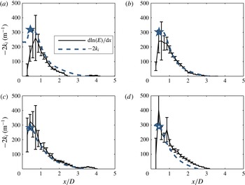
Figure 9 also shows that the amplitude of the oscillations increases in the absolutely unstable region and that the maximum spatial growth rate coincides approximately with the point of maximum absolute instability. This can be examined more precisely by comparing the spatial growth rate from the local analysis with that from the experimental measurements. In order to obtain the spatial growth rate from experiments, we assume a linear normal-mode form for the streamwise and transverse global mode velocity components,
 $(u,v)=(|\hat{u} |,|\hat{v}|)\exp [-\text{i}({\it\omega}t-kx)]$
. Next, we recall that the global mode energy has the general form
 $E=\int _{0}^{H}(|u|^{2}+|v|^{2})\,\text{d}y$
. Finally, we differentiate to obtain the spatial growth rate,
 $-2k_{i}=\text{d}\ln (E)/\text{d}x$
. Figure 12 compares the streamwise dependence of the spatial growth rate derived from the local analysis (solid line) and from the experiments (dashed line). The spatial growth rates from the local analysis are composed of the
 $k^{+}$
and
 $k^{-}$
branches, computed for the predicted global mode frequency,
 $f_{g,l}$
. The
 $k^{-}$
branch is selected in the region upstream of the wavemaker, and the
 $k^{+}$
branch is selected downstream of the wavemaker. In a local analysis around a steady flow, the two should match well in the low-amplitude region upstream, where the growth is linear, but would not be expected to match in the high-amplitude region downstream. In the local analysis around the time-averaged flow shown here, however, the two match reasonably well upstream (particularly for the
 $U_{lip}=60$
cases) but match even better in the high-amplitude region downstream. This shows that, given a mean flow, the linear local analysis can predict the local spatial growth rate and therefore is likely to give a correct mode shape. Although this is something of a circular argument, because the mean flow was generated from the mode shape in the first place, it is reassuring for the next stage in this analysis, which is to calculate the direct and adjoint global modes from the local linear analysis.
Recalling the nonlinear wave-front theory of Pier & Huerre (Reference Pier and Huerre1996), the measured and predicted linear spatial growth rates are expected to match at the point where the flow transitions from convective to absolute instability. Figure 12 identifies this point with a
 $\star$
symbol. The figure shows a good match between experiment and prediction at this point for the 60 m s
 $^{-1}$
cases, and a poorer match for the 30 m s
 $^{-1}$
cases. The reason for the poor comparison (as well as for the scatter in the nonlinear wave-front frequencies in figure 8
b) is unknown, but the authors suspect that it is due to the higher measurement uncertainty of the fluctuating velocity at this spatial position (as quantified by the error bars).
Comparison of predicted linear spatial growth rate to measured spatial growth rate:
 ${\it\rho}_{u}/{\it\rho}_{b}=2$
(a,c); 1.7 (b,d);
 $U_{lip}=30$
m s
 $^{-1}$
(a,b); 60 m s
 $^{-1}$
(b,d). Symbol
 $\star$
is placed at the streamwise position where linear stability analysis predicts the transition from convective to absolute instability (the upstream boundary of the pocket of absolute instability). The error bars represent PIV measurement uncertainty due to the Stokes number considerations discussed in § 3.2.

This section showed comparisons between stability analysis predictions using an experimentally measured base flow, and the experimentally measured flow oscillations. The comparisons show good qualitative trends in the predictions, with small quantitative discrepancies. Three sources of error may account for these discrepancies. These potential sources of error, discussed in detail in §§ 2 and 3.2, are uncertainty in the measured base flow (which propagates through the stability analysis), errors inherent to the stability analysis procedure, and uncertainty in the measured oscillatory velocity. Experimental uncertainty in the oscillatory frequency is extremely small, and uncertainty in the oscillatory velocity amplitude is quantified and indicated with error bars. The authors hypothesize that discrepancies beyond these error bars are due to errors that are inherent to the stability analysis, not due to the small uncertainty in the measured base flow. The weakest components of the analysis procedure are the parallel-flow assumption, and the use of a time-averaged turbulent flow field as the base flow. The influence of the parallel-flow assumption could be investigated in future work with a full global analysis.
5.2. Direct global mode, adjoint global mode, and wavemaker
The aim of this section is to compare the predicted (linear) 2D global mode shape to the measured (nonlinear) 2D global mode shape, and to obtain the adjoint global mode and the eigenvalue sensitivity,
 ${\it\lambda}$
. This analysis, which is performed around the time-averaged mean flow, is similar to that of Meliga et al. (Reference Meliga, Pujals and Serre2012), which included a frozen eddy viscosity, and Mettot et al. (Reference Mettot, Sipp and Bezard2014), which used only molecular viscosity. These analyses were compared with the experimentally derived sensitivities by Parezanovic & Cadot (Reference Parezanovic and Cadot2012) and found to give excellent predictions of the oscillation’s sensitivity to the addition of a passive-control element.
The measured global mode shape is obtained by conditionally averaging the velocity field at a fixed phase of the global mode oscillation. To accomplish this, the mean-subtracted transverse velocity time series from a single spatial point is locally fitted to a sinusoid with a fixed frequency of
 $f_{n}=0.24U_{lip}/D$
over two period windows (Emerson et al.
Reference Emerson, O’Connor, Juniper and Lieuwen2012). The phases of these sinusoidal fits are stored as a time-dependent signal. This signal is then used as a reference phase to conditionally average the entire velocity field at instants that correspond to a fixed reference phase.
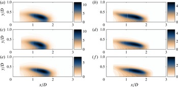
Sinuous mode shape, showing from (a) to (e): instantaneous measured global mode showing conditionally averaged transverse velocity, instantaneous linear direct global mode shape showing transverse velocity,
 $v$
, adjoint global mode showing receptivity to streamwise velocity forcing,
 $|u^{\dagger }|$
, adjoint global mode showing receptivity to transverse velocity forcing,
 $|v^{\dagger }|$
, and eigenvalue sensitivity,
 ${\it\lambda}$
. Conditions are
 ${\it\rho}_{u}/{\it\rho}_{b}=1.7$
,
 $U_{lip}=30$
m s
 $^{-1}$
.

Phase speed (a) and phase velocity (b) of the experimentally measured and the predicted mode shapes of the fluctuating transverse velocity. Conditions are
 ${\it\rho}_{u}/{\it\rho}_{b}=1.7$
,
 $U_{lip}=30$
m s
 $^{-1}$
.

An example snapshot (i.e. a single phase) of the conditionally averaged transverse velocity is shown in figure 13(a) for the upper half of the channel. The direct global mode shape is presented in the frame immediately below. Comparison between these two shows qualitatively similar transverse mode shapes. For a more quantitative comparison of the global mode to the experimental measurement, figure 14 compares the axial dependences of the phases of the linear global mode and conditionally averaged transverse velocity. The experimentally measured phase was determined by first performing a fast Fourier transform (FFT) of the transverse velocity at every spatial position. Next, the phase was extracted from the transverse-velocity Fourier coefficients,
 $\hat{v}$
, at the global mode frequency,
 $f_{g,m}$
, and at a transverse position of
 $y/D=0$
. As such, for the experimental measurement, we define the phase as
 ${\it\theta}(x)=\angle \hat{v}(x,y/D=0,f=f_{g,m})$
. For both the stability analysis and the experimental measurement, figure 14(b) shows the phase speed, which is representative of the convective velocity, and which is calculated from finite differencing the axial dependence of the phase. The phase speed is calculated as
 $$\begin{eqnarray}U_{c}(x)=2{\rm\pi}f_{g}\frac{{\rm\Delta}x}{{\rm\Delta}{\it\theta}},\end{eqnarray}$$
where
 ${\rm\Delta}x$
represents a finite difference of the axial position, and
 ${\rm\Delta}{\it\theta}$
represents a finite difference of the phase. The figure shows that the linear stability analysis captures the qualitative trend of an accelerating phase speed with increasing axial position. Additionally, the figure shows close quantitative agreement, although the stability analysis appears to slightly overpredict the phase speed. This overprediction of the phase speed is also evident in figure 13, which suggests a slightly longer axial wavelength for the prediction, relative to the experiment. As a quantitative comparison of the magnitudes of the predicted and measured global modes, the reader is referred to the spatial growth rates plotted in figure 12, which shows the same case as figures 13 and 14.
The adjoint global modes for streamwise and transverse velocity perturbations are shown in figure 13(c,d). These quantify the influence that open-loop velocity forcing has on the oscillation amplitude, as shown by the final term in equation (9) of Chomaz (Reference Chomaz2005). For example, this shows that the global mode is most sensitive to open-loop velocity forcing in the shear layers aft of the bluff body and that it is slightly more sensitive to streamwise forcing than transverse forcing. Finally, the eigenvalue sensitivity,
 ${\it\lambda}$
, is shown in the last frame. The values of
 ${\it\lambda}$
shown here are the products of the direct and adjoint global mode velocity magnitudes,
 ${\it\lambda}=\sqrt{|u|^{2}+|v|^{2}}\times \sqrt{|u^{\dagger }|^{2}+|v^{\dagger }|^{2}}$
. This quantity physically represents the eigenvalue drift caused by a device that produces an extra acceleration (i.e. momentum feedback) at a given point in space. This is large in locations that have both significant oscillation amplitude (contained in the direct global mode) and significant sensitivity to oscillations (contained in the adjoint global mode), and therefore identifies the location where a passive-feedback device would have most influence if it affects the perturbation but not the base flow. This is the wavemaker region of the flow. Notice that for this flow, the wavemaker is located in the recirculation zone of the wake, between
 $x/D=1$
and
 $x/D=2$
.
This study pursues the eigenvalue sensitivity to momentum feedback, defined above as
 ${\it\lambda}$
. However, it is important to note that there are many different ways to define the eigenvalue sensitivity, each of which describes the eigenvalue drift caused by a different type of feedback. As a practical example, the quantity
 ${\it\lambda}/{\it\rho}_{0}$
would physically represent the eigenvalue drift due to a device that causes an extra force feedback at a point in space. Although not shown here for reasons of space, analysis of this scenario reveals a nearly identical wavemaker region, due to the fact that the wavemaker region lies almost entirely in the uniform-density combustion-products region.
Comparison of the sinuous mode eigenvalue sensitivity,
 ${\it\lambda}$
, for several velocities and density ratios:
 $U_{lip}=30$
m s
 $^{-1}$
(a,c,e); 60 m s
 $^{-1}$
(b,d,f);
 ${\it\rho}_{u}/{\it\rho}_{b}=1.7$
(a,b); 1.9 (c,d); 2.0 (e,f).

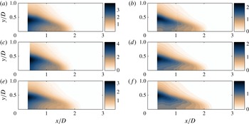
Comparison of the sinuous mode receptivity to transverse velocity forcing,
 $|v^{\dagger }|$
, for several velocities and density ratios:
 $U_{lip}=30$
m s
 $^{-1}$
(a,c,e); 60 m s
 $^{-1}$
(b,d,f);
 ${\it\rho}_{u}/{\it\rho}_{b}=1.7$
(a,b); 1.9 (c,d); 2.0 (e,f).

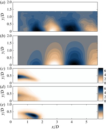
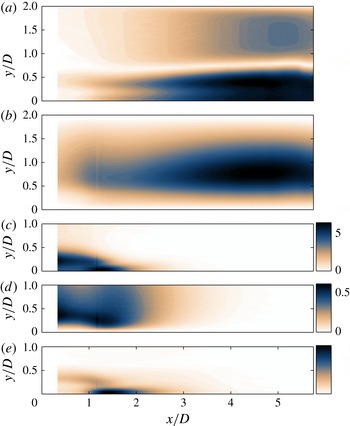
Varicose mode shape, showing from (a) to (e): direct streamwise velocity global mode,
 $u$
, direct transverse velocity global mode,
 $v$
, adjoint global mode showing receptivity to streamwise velocity forcing,
 $|u^{\dagger }|$
, adjoint global mode showing receptivity to transverse velocity forcing,
 $|v^{\dagger }|$
, and eigenvalue sensitivity,
 ${\it\lambda}$
. Conditions are
 ${\it\rho}_{u}/{\it\rho}_{b}=1.7$
,
 $U_{lip}=30~\text{m}~\text{s}^{-1}$
. Colour bar for
 $|v^{\dagger }|$
is
 $1/10$
th the colour bar of
 $|u^{\dagger }|$
for visibility purposes.

5.3. Influence of density ratio and lip velocity on wavemaker region and receptivity regions
Figure 15 presents a comparison of the wavemaker region for three density ratios and two lip velocities. The left-hand column is a density-ratio sweep at a fixed lip velocity of
 $U_{lip}=30$
m s
 $^{-1}$
, and the right-hand column is a density-ratio sweep at a fixed lip velocity of
 $U_{lip}=60$
m s
 $^{-1}$
. The figure shows that the wavemaker shape and location are relatively insensitive to these two parameters, even though the growth rates, frequencies, and amplitudes vary significantly, as shown earlier. The most noticeable influence is the slight elongation of the wavemaker region with increases in bluff-body lip velocity. There also appears to be a slight elongation of the wavemaker region with increase in density ratio, which is apparent when comparing the
 ${\it\rho}_{u}/{\it\rho}_{b}=1.7$
cases to the
 ${\it\rho}_{u}/{\it\rho}_{b}=2.0$
cases. These effects are probably due to the slight increase in recirculation zone length with increases in lip velocity and density ratio (Emerson et al.
Reference Emerson, O’Connor, Juniper and Lieuwen2012), and support the observation from the end of § 5.2, as well as that from analyses around steady flows (Giannetti & Luchini Reference Giannetti and Luchini2007), that the wavemaker is centred on the recirculation zone.
Figure 16 presents a comparison of the receptivity to transverse velocity forcing (the adjoint mode). This region follows the edge of the time-averaged recirculation region, which varies slightly as the lip velocity and density ratio change.
5.4. Varicose oscillations
The previous sections concerned the sinuous mode, which is the observed wake mode in the absence of external forcing or thermoacoustic oscillations. However, varicose oscillations may be excited by external forcing. For example, experimental work by Emerson et al. (Reference Emerson, Murphy and Lieuwen2013) demonstrated that varicose oscillations often dominate in longitudinal combustion instabilities of bluff-body combustors. Therefore, the stability of the varicose mode has direct application to the combustion-instability problem. While the stability analysis does not model the acoustically coupled global thermoacoustic system, it does reveal the most significant sensitivities of the hydrodynamic component of such a system, from which one may speculate about the overall system. For example, figure 17 will show that the hydrodynamic response to acoustic driving is much more sensitive to streamwise forcing than to transverse forcing, and that the highest eigenvalue sensitivity sits on the flow centreline just downstream of the bluff body. For this reason, this section explores the stability of varicose oscillations around the time-averaged flow calculated from the experimental data.
It is worth noting that the predominant unsteady feature in the experimental data is a sinuous mode. Therefore, this analysis is pertinent to varicose oscillations occurring on top of a flow that is already oscillating sinuously. An important point when considering a linear interpretation of such a situation is for the two modes to oscillate independently at different time scales. For the conditions presented in this section (
 ${\it\rho}_{u}/{\it\rho}_{b}=1.7$
,
 $U_{lip}=30~\text{m}~\text{s}^{-1}$
), the predicted frequency of the varicose global mode is 35 Hz, which is an order of magnitude lower than the 374 Hz frequency predicted for the sinuous global mode.
Figure 17 shows (a,b) the direct global mode, (c,d) the receptivities to streamwise and transverse velocity forcing, and (e) the wavemaker of the varicose mode. The varicose mode shown in figure 17 was computed for the same base flow as the sinuous mode shown previously in figure 13. Comparing these two figures reveals some significant differences between the sinuous and varicose modes.
Firstly, the streamwise wavelength of the varicose direct global mode is much longer than that of the sinuous mode. Evidence of this has been observed previously in the direct numerical simulations of Biancofiore et al. (Reference Biancofiore, Gallaire, Laure and Hachem2014). Secondly, by comparing the relative amplitudes of the (c) streamwise and (d) transverse receptivities in figures 16 and 17, it can be seen that the varicose mode is much less sensitive to transverse forcing than the sinuous mode. Thirdly, although the varicose mode is similar to the sinuous mode in that it is very receptive to forcing in the shear layers, it is also receptive to streamwise velocity forcing along the centreline around
 $x/D=1$
. This implies that the growth rate of the varicose oscillations could be reduced (or the damping rate increased) by streamwise injection from the body at
 $y/D=0$
, while minimally affecting the sinuous oscillation. In a system that is forced in a varicose manner, e.g. by thermoacoustic oscillations, this would reduce the amplitude of the hydrodynamic oscillations and thereby weaken the feedback mechanism between the acoustics and heat release. Fourthly, the wavemaker region of the varicose mode has highest amplitude at
 $y/D=0$
, while that of the sinuous mode is at
 $y/D=0.25$
. Additionally, there is a separate distinct weaker wavemaker region in the shear layer. This tendency of the varicose mode to have two distinct receptivity regions and wavemaker regions was not present in the sinuous mode, and is consistent when varying
 ${\it\rho}_{u}/{\it\rho}_{b}$
and
 $U_{lip}$
.
6. Conclusions
This study examines the receptivity and sensitivity of the oscillating flow behind a flame holder in the presence of combustion. A local stability analysis is used in order to calculate the direct and adjoint linear global modes about the experimentally derived time-averaged base flow. This procedure has been applied to laminar nonreacting wakes (Juniper & Pier Reference Juniper and Pier2015) and has been shown to give a very good approximation to the modes found from a global analysis, particularly for nearly parallel flows such as this.
The direct global modes calculated from the local stability analysis have similar frequencies, mode shapes, phase speeds, and streamwise growth rates as the experimentally observed oscillations over a wide range of flame-density ratios and bluff-body lip velocities. This provides a sound basis on which to form the adjoint global modes for the receptivity and sensitivity analysis. In addition, the linear local analysis predicts a global growth rate that is proportional to the square of the experimentally measured amplitude of oscillation, in accordance with a Stuart–Landau model. This feature was not found in the linear global analyses of Barkley (Reference Barkley2006), Meliga et al. (Reference Meliga, Pujals and Serre2012), Mettot et al. (Reference Mettot, Sipp and Bezard2014), which were also around the time-averaged mean flow.
The adjoint global modes show where the flows are most receptive to external forcing. For sinuous oscillations, the flow is slightly more receptive to streamwise forcing than to transverse forcing and is most receptive in the shear layers just downstream of the bluff-body edges. For varicose oscillations, the flow is much more receptive to streamwise forcing than to transverse forcing. It is quite receptive in the shear layers, but it is most receptive along the centreline, although only to streamwise forcing. The overlap of the direct and adjoint global modes shows where the flows are most sensitive to changes in internal feedback, which is the wavemaker region. For both sinuous and varicose oscillations, this region is at around
 $x/D=1.5$
.
The regions of high receptivity and sensitivity change very little as the density ratio and lip velocity change. However, the stability analysis shows that increasing the density ratio reduces the global mode growth rate and has little influence on the global mode frequency. This stabilizing influence is reflected in the experiments, in which the limit-cycle amplitude reduces when the density ratio increases. The stability analysis also shows that increasing the bluff-body lip velocity causes a proportional increase in the global mode frequency, which compares well with the experimentally measured global mode frequency.
This study performs a local stability analysis on experimentally derived time-averaged velocity profiles in a slowly developing wake flow. The authors implement the techniques described in Juniper & Pier (Reference Juniper and Pier2015) to extract the direct and adjoint global modes from the local analysis. These modes show the regions of the flow that are most receptive to external forcing and sensitive to changes in internal feedback. For the combusting flow behind a bluff body studied here, this analysis shows that the sinuous mode is more hydrodynamically unstable than the varicose mode and that the varicose mode has a much lower frequency and longer wavelength. Nevertheless, the varicose mode can lock into longitudinal oscillations in practical combustion systems and thereby cause thermoacoustic oscillations. The varicose mode is quite receptive to momentum forcing in the shear layers downstream of the bluff body. A longitudinal acoustic mode would have high amplitude in these regions, which reveals how this type of acoustics couples to the flame effectively. The varicose mode is most receptive to streamwise momentum forcing along the centreline, however, where the sinuous mode is insensitive to forcing. This provides physical insight into the reasons behind the behaviour of this flow, and suggests a control strategy involving streamwise forcing behind the bluff body, either with feedback control or with a passive device. Such a strategy might change the varicose mode, which is dangerous for thermoacoustics, without affecting the sinuous mode, which is good for mixing.
Acknowledgements
M.P.J. acknowledges the financial support of the European Research Council under grant no. 2590620. T.L. acknowledges the support of the University Turbine Systems Research program (contract no. DE-FC21-92MC29061), under contract monitor Dr M. Freeman, and the Air Force Office of Scientific Research (contract no. FA9550-12-1-0107/RC657), under contract monitor Dr C. Lee.