



1 Introduction
The dynamics of swirling flows in a pipe, specifically at high levels of rotation, is dominated by flow instabilities and the vortex breakdown phenomenon (see the experimental studies of Sarpkaya (Reference Sarpkaya1971, Reference Sarpkaya1974), Faler & Leibovich (Reference Faler and Leibovich1977), Garg & Leibovich (Reference Garg and Leibovich1979), Brucker & Althaus (Reference Brucker and Althaus1995), Malkiel et al. (Reference Malkiel, Cohen, Rusak and Wang1996), Mattner, Joubert & Chong (Reference Mattner, Joubert and Chong2002), Liang & Maxworthy (Reference Liang and Maxworthy2005), Umeh et al. (Reference Umeh, Rusak, Gutmark, Villalva and Cha2010) and Dennis, Seraudie & Poole (Reference Dennis, Seraudie and Poole2014)). The instabilities range from various types of helical waves to the major types of breakdown, the axisymmetric bubble and the spiral breakdown. Understanding the onset of these instabilities can shed light on the vortex breakdown phenomenon which either limits the flight of airplanes operating at high angles of attack or is used in modern combustion chambers as a natural flame holder to stabilize the flame. Currently, there is no general consensus in the literature that vortex breakdown describes a single phenomenon.
Reviews of the vortex breakdown phenomenon include the papers by Hall (Reference Hall1972), Leibovich (Reference Leibovich1984) and Ash & Khorrami (Reference Ash, Khorrami and Green1995). Several theories have been advanced over the years to explain various aspects or mechanisms of the vortex breakdown phenomenon. These include the studies by Benjamin (Reference Benjamin1962), Randall & Leibovich (Reference Randall and Leibovich1973), Keller, Egli & Exley (Reference Keller, Egli and Exley1985) and Leibovich & Kribus (Reference Leibovich and Kribus1990) who investigated the dynamics of standing or travelling nonlinear axisymmetric waves on swirling flows in an infinitely long straight pipe model. We note however that the case of a flow in an infinitely long straight pipe pertains to a translational invariance, but such an entity does not exist in the experimental apparatuses.
Extensive studies have focused on the numerical simulation of vortex breakdown states including the papers by Spall & Gatski (Reference Spall and Gatski1991), Spall (Reference Spall1996), Tromp & Beran (Reference Tromp and Beran1997) and Cary, Darmofal & Powell (Reference Cary, Darmofal and Powell1997). They computed the evolution of various three-dimensional perturbations and the formation of either axisymmetric or spiral breakdown states. They also simulated the possible transition from a spiral wave to an axisymmetric bubble and from a bubble breakdown to a spiral breakdown.
In a seminal comprehensive numerical simulation, Ruith et al. (Reference Ruith, Chen, Meiburg and Maxworthy2003) focused on the instability of a base axisymmetric breakdown state in a long finite axial domain. Their simulation revealed for the first time the details of the onset of a linear spiral instability mode in the axisymmetric breakdown state that grows in size and evolves to a rotating spiral breakdown wave behind a perturbed axisymmetric bubble. They also tried to explain this instability using a weakly non-parallel flow assumption and testing the convective instability (CI) – absolute instability (AI) of various cross-sections around the breakdown bubble to determine the CI–AI transition and the AI zone at the rear part of the breakdown bubble. However, they found that this approach is limited in scope and accuracy in describing the spiral instability mode since the base axisymmetric breakdown state is definitely not a weakly non-parallel flow. Moreover, the CI–AI analysis does not account for the interaction of flow perturbations with the active upstream and passive downstream states. These concerns motivated Ruith et al. (Reference Ruith, Chen, Meiburg and Maxworthy2003) to characterize the growing linear spiral instability mode using the direct numerical simulation (DNS).
Gallaire et al. (Reference Gallaire, Ruith, Meiburg, Chomaz and Huerre2006) attempted to refine the CI–AI calculations of the base axisymmetric breakdown state that Ruith et al. (Reference Ruith, Chen, Meiburg and Maxworthy2003) conducted. Their results found a finite pocket of AI attached to the rear part of the breakdown bubble. However, they did not establish any prediction of the properties of the shape, growth rate and frequency of rotation of the linear spiral mode of instability that was found by Ruith et al. (Reference Ruith, Chen, Meiburg and Maxworthy2003).
Recently, Jones, Hourigan & Thomson (Reference Jones, Hourigan and Thomson2015) used direct numerical simulations to construct a dividing line for the occurrence of the various types of vortex breakdown in a Reynolds number versus swirl level operational diagram. This dividing line indicates that possible instabilities develop on the base swirling flow at operational conditions where vortex breakdown states are found. However, they did not study the linear stability of the base flow and its relationship to the breakdown process.
The classical vortex stability theory (Kelvin Reference Kelvin1880; Rayleigh Reference Rayleigh1916; Synge Reference Synge1933; Howard & Gupta Reference Howard and Gupta1962; Lessen & Paillet Reference Lessen and Paillet1974; Lessen, Singh & Paillet Reference Lessen, Singh and Paillet1974; Leibovich & Stewartson Reference Leibovich and Stewartson1983) studied the dynamics of axial normal periodic perturbation modes of a base swirling flow. Such a study however is strictly valid only for a columnar swirling flow in an infinitely long straight pipe or in a finite-length pipe with periodic inlet–outlet conditions and it necessarily preserves a translational invariance. This limitation has been overlooked for a long time and the Rayleigh stability criterion that is related to the base flow circulation monotonicity was thought to be applicable for any vortex flow in a pipe.
The stability and global analyses of Wang & Rusak (Reference Wang and Rusak1996, Reference Wang and Rusak1997) were the first to reveal this crucial limitation of the classical flow stability theory. They proposed a set of non-periodic inlet–outlet conditions and revealed a completely different mode analysis that is able to describe the physics of swirling flows in a finite-length pipe where the translational invariance does not exist (also see Wang & Rusak Reference Wang and Rusak2011). They showed the existence of an axisymmetric non-Fourier mode of perturbation that becomes unstable when the incoming flow swirl level is above a certain critical level. The growing perturbation evolves through a faster-than-exponential nonlinear mode to an axisymmetric breakdown state that is a global minimum state of the flow force at the given incoming flow swirl level (see Rusak et al. Reference Rusak, Wang, Xu and Taylor2012). This instability mode results from the strong axial inhomogeneity between the active inlet and passive outlet states of the flow in a finite-length open pipe and cannot be explained by either the classical stability theory or the CI–AI analysis. The Wang & Rusak (Reference Wang and Rusak1996, Reference Wang and Rusak1997) analyses are consistent with a swirling flow behaviour in the experimental apparatuses mentioned above where the swirling flow domain is of finite size and an axisymmetric perturbation evolves to an axisymmetric breakdown state.
In a recent paper, Wang et al. (Reference Wang, Rusak, Gong and Liu2016) have analysed the three-dimensional, inviscid and viscous flow instability modes that appear in a solid-body rotation flow in a finite-length, straight, circular pipe. Their study is a direct extension of the Wang & Rusak (Reference Wang and Rusak1996) analysis of axisymmetric (
 $m=0$
) instabilities for inviscid swirling flows in a pipe. A general mode of perturbation for the linearized flow problem has been considered. It is composed of an azimuthal normal mode (with either
 $m=0$
or
 $m\neq 0$
azimuthal wavenumber) and a non-axial Fourier mode in the radial and axial coordinates. The results have shown that the fundamental root cause for the existence of axisymmetric and three-dimensional instabilities in swirling flows in pipes is the elimination of the flow axial homogeneity due to the essential asymmetric role of the active inlet state and the passive outlet state in a convective flow system of finite size. At high swirl ratios, the high level of confined kinetic energy in the swirling flow can be triggered to be released through various physical agents that eliminate the axial homogeneity along the pipe and form either axisymmetric (
 $m=0$
) or spiral (
 $m=1,2,\ldots$
) instability modes that appear in sequence and with higher growth rates as the swirl ratio is increased. Such physical agents include a flow set-up with the inlet conditions behind a fixed-in-time and fixed-in-space vortex generator and an outlet passive discharge device. Viscosity or pipe geometry divergence/contraction can also generate significant axial inhomogeneity. The stability results of Wang et al. (Reference Wang, Rusak, Gong and Liu2016) have been summarized in a Reynolds number (
 $Re$
) versus swirl level (
 $\unicode[STIX]{x1D714}$
) operational diagram which clearly shows the dividing line between stable and unstable swirling flows and the range of operational parameters for either dominant axisymmetric modes or for dominant spiral instability modes. This diagram provides guidelines for the occurrence of such instabilities. The results have indicated the various possible dynamics of perturbations in swirling flows that may lead to either the axisymmetric or the spiral types of breakdown.
The linear stability analyses of Wang & Rusak (Reference Wang and Rusak1996) and Wang et al. (Reference Wang, Rusak, Gong and Liu2016) also indicate a direct relationship between flow strong axial inhomogeneity in a finite-size domain and the linear instability spiral mode of the axisymmetric breakdown state first discovered by Ruith et al. (Reference Ruith, Chen, Meiburg and Maxworthy2003). The base state of an axisymmetric breakdown bubble also forms a significant flow radial expansion and a strong axial inhomogeneity and, together with the inhomogeneity from the upstream and downstream conditions, leads to instability modes that cannot be explained by either the classical vortex stability theory (based on normal mode analysis) or its extension using a weakly non-parallel flow CI–AI analysis. In fact, only when Meliga & Gallaire (Reference Meliga and Gallaire2011) performed a linear stability analysis of the base axisymmetric breakdown state of Ruith et al. (Reference Ruith, Chen, Meiburg and Maxworthy2003) with the same boundary conditions as in the simulation, were they able to accurately reproduce the characteristics of the linear spiral instability mode as calculated by Ruith et al. (Reference Ruith, Chen, Meiburg and Maxworthy2003). This demonstrates the importance of including all flow boundary conditions in determining flow instabilities in a finite-size domain.
In this paper we study via direct numerical simulations the three-dimensional, incompressible and viscous flow dynamics of perturbations on a base solid-body rotation flow with a uniform axial velocity entering a rotating, finite-length, straight circular pipe. The simulation results provide the neutral stability line in response to either axisymmetric or three-dimensional perturbations in a
 $Re$
versus
 $\unicode[STIX]{x1D714}$
operational diagram. This line is found to be in good agreement with the neutral stability line predicted by the linear stability analysis of Wang et al. (Reference Wang, Rusak, Gong and Liu2016). The present study also shows various types of flow evolution scenarios. First, the Wang & Rusak (Reference Wang and Rusak1996, Reference Wang and Rusak1997) axisymmetric instability mechanism and evolution to a stable axisymmetric breakdown state is recovered in the simulations at certain operational conditions in terms of
 $Re$
and
 $\unicode[STIX]{x1D714}$
. However, at other operational conditions with the same
 $\unicode[STIX]{x1D714}$
but with a higher
 $Re$
, we find a second scenario. The breakdown state, that was initiated by an axisymmetric instability of the base columnar flow, continues to evolve and a spiral instability mode appears on it and grows to a rotating spiral breakdown state. The mechanism of this process is shown to be the same as that of the axisymmetric instability discovered by Wang & Rusak (Reference Wang and Rusak1996). In this case the axisymmetric bubble enhances the axial inhomogeneity of the flow to form a spiral instability mode. It is noticed that this case is similar to the case studied in the simulations of Ruith et al. (Reference Ruith, Chen, Meiburg and Maxworthy2003), thus the unstable spiral linear mode of the axisymmetric breakdown state discovered in their study can be attributed to the same mechanism, i.e. it is caused essentially by the loss of axial flow homogeneity. Moreover, at higher levels of
 $\unicode[STIX]{x1D714}$
we find a third scenario where there exists a dominant three-dimensional spiral type of instability mode that agrees with the linear stability theory of Wang et al. (Reference Wang, Rusak, Gong and Liu2016). The growth of this mode leads directly to a spiral type of flow roll up that subsequently nonlinearly saturates in a rotating spiral type of vortex breakdown. This distinct breakdown process was never studied.
Following Ruith et al. (Reference Ruith, Chen, Meiburg and Maxworthy2003), the numerically simulated global dynamical scenarios described above are studied by flow snapshots of streaklines and related low-dimensional representations of the dynamics in phase portraits of the trajectories of the velocity components at a certain point in the domain (§ 4). All streaklines are constructed by following massless particles continuously released in time at the pipe inlet
 $x=0$
on a circle with radius
 $r=0.05$
. In addition, a conclusive energy transfer mechanism between the perturbation and the base flow that is based on the Reynolds–Orr equation has been conducted to reveal the underlying physical mechanism that drives all the various flow instabilities and transitions to breakdown states. These global analysis tools lead to a consistent and conclusive explanation of the various processes of the vortex breakdown phenomenon and the stabilization of various breakdown states.
We emphasize the importance of using the solid-body rotation flow with a uniform axial velocity as the base flow for the present study. According to the Kelvin (Reference Kelvin1880) inviscid flow stability analysis, this base flow is neutrally stable to all normal mode perturbations. Since the linearized stability problem results in orthogonal modes, there are also no transient instability modes with this base flow. Therefore, the onset of instability modes found in this paper is definitely not related to CI–AI analysis. As shown through the use of the Reynolds–Orr equation in § 5, the instability modes we found are directly related to the strong axial inhomogeneity induced by the inlet and outlet flow states while the base flow in the bulk affects the growth of perturbation only through viscous dissipation effects.
Moreover, we also conduct in § 6 an energy analysis based on the Reynolds–Orr equation where the base flow is an axisymmetric breakdown state. We reveal that the spiral instability mode of this state is also dominated by the flow strong axial inhomogeneity. In addition, the total contribution of this base non-parallel flow to the production of the perturbations’ kinetic energy in the bulk is negative and actually induces the decay of the perturbations. Only when the inlet and outlet terms induced by the strong inhomogeneity of the boundary states are added to the production terms, is the perturbation found to be unstable. This analysis also demonstrates that the results of the present paper and the mechanism of vortex breakdown are not limited to only the base solid-body rotation flow in a finite-length pipe but are general in scope to the stability of any vortex flow and the transition to breakdown states in a finite-size domain. The instability is directly caused by the strong non-parallel flow effect due to the convective flow nature and its confinement effect, which definitely cannot be revealed by a CI–AI analysis that is based on a weakly non-parallel flow assumption. Thereby, the present analysis also sheds new light on the mechanism of the instability described in Ruith et al. (Reference Ruith, Chen, Meiburg and Maxworthy2003).
The present study focuses on the case of a solid-body rotating flow in a pipe of non-dimensional length
 $L=2$
(length of one diameter). For this case, the mechanism of flow instability and breakdown, either axisymmetric or three-dimensional spiral, is firmly established. This canonical model of flow set-up can be realized in experiments and is a well selected model to reveal the physical nature of the instabilities as related to strong non-parallel flow effects and axial flow inhomogeneity, that are not related to the AI–CI concept. Moreover, as revealed by the Reynolds–Orr equation, all of the instabilities are accurately evaluated by the difference of energy production inside of the domain and at the boundary. This adds substantial confidence to the presented results.
Moreover, our previous theoretical studies and simulations in Wang & Rusak (Reference Wang and Rusak1996, Reference Wang and Rusak1997), Rusak, Wang & Whiting (Reference Rusak, Wang and Whiting1998) and Rusak et al. (Reference Rusak, Wang, Xu and Taylor2012) already established this mechanism for axisymmetric flows of general vortices in a pipe with non-dimensional length
 $L=6$
. Studying the quantitative effect of pipe length on the instability mechanism and vortex dynamics in longer pipes is an important research subject which requires an extensive investigation of several pipe lengths: for example, from
 $2$
to
 $20$
. For a detailed quantitative characteristics of flow stability and dynamics, each case of pipe length requires simulations at various combinations of Reynolds numbers and swirl levels. Such an extensive study is beyond the scope of this paper. In fact, the length
 $L=2$
was chosen in this study because it is computationally efficient to conduct the simulations and to reveal the strong non-parallel flow effect. In addition, the comparison of the present neutral stability results for
 $L=2$
and the results computed from the linear stability analysis in Wang et al. (Reference Wang, Rusak, Gong and Liu2016) shows similarity between the cases. The essential difference between these cases is that the
 $L=2$
case shows well-separated stability/instability modes and it thus requires the least computational power to reveal through simulations the transition to breakdown states in response to the various instability modes. However, due to the physical sensitivity of the case with
 $L=6$
to the appearance of many instability modes with the slight increase of the inlet swirl level, the simulations to determine the long-term dynamics of the flow must be undertaken with much more care (the use of very small steps of the swirl level) and require a much higher computational cost due to a much more refined mesh.
The paper outline is as follows. The mathematical model and numerical method used in the simulations are discussed in § 2. Section 3 presents the results of three-dimensional numerical simulations and their analyses with respect to the linear stability results of Wang et al. (Reference Wang, Rusak, Gong and Liu2016). Streakline contours and phase portraits of the velocity components at a fixed point in the domain are used to shed light on the relationship between the base flow linear stability, the flow global dynamics and its long-term behaviour. Section 4 describes in a systematic way the various scenarios of rich dynamics of the flow in the operational map of
 $\unicode[STIX]{x1D714}$
against
 $Re$
. Section 5 uses the Reynolds–Orr equation to reveal the mechanism of the various instabilities and transitions to the breakdown states. We also give a detailed discussion that shows that there is no relationship between the instabilities we found and a CI–AI analysis (§ 6). Section 7 summarizes the conclusions of this study.
2 Mathematical model and numerical simulation method
We consider an incompressible and viscous swirling flow in a straight, finite-length, circular pipe of radius
 $R$
and length
 $LR$
, where
 $L$
is the pipe non-dimensional length. The non-dimensional cylindrical coordinates
 $(r,\unicode[STIX]{x1D703},x)$
are used where
 $x$
measures axial distance from the pipe inlet at
 $x=0$
,
 $r$
measures radial distance from the pipe centreline and
 $0\leqslant \unicode[STIX]{x1D703}<2\unicode[STIX]{x03C0}$
. The axial and radial distances are rescaled by the pipe radius
 $R$
. The velocity components
 $u_{r}$
,
 $u_{\unicode[STIX]{x1D703}}$
and
 $u_{x}$
are the radial, azimuthal and axial velocities, respectively, and they are scaled by a characteristic axial velocity at the pipe inlet,
 $U$
. Time
 $t$
is rescaled with
 $R/U$
. The pressure field is denoted as
 $p$
and is scaled by
 $\unicode[STIX]{x1D70C}U^{2}$
. The flow constant density and viscosity are
 $\unicode[STIX]{x1D70C}$
and
 $\unicode[STIX]{x1D707}$
, respectively.
To avoid computational singularity along the centreline of the pipe, we use the vector
 $\boldsymbol{q}=(q_{r},q_{\unicode[STIX]{x1D703}},q_{x})$
where
 $q_{r}=ru_{r}$
,
 $q_{\unicode[STIX]{x1D703}}=ru_{\unicode[STIX]{x1D703}}$
and
 $q_{x}=u_{x}$
, respectively. The flow evolution in the domain
 $0\leqslant x\leqslant L,~0\leqslant r\leqslant 1,0\leqslant \unicode[STIX]{x1D703}<2\unicode[STIX]{x03C0}$
is described for all
 $t\geqslant 0$
by the unsteady, three-dimensional Navier–Stokes equations in cylindrical coordinates:
 $$\begin{eqnarray}\displaystyle & \displaystyle {\displaystyle \frac{1}{r}}{\displaystyle \frac{\unicode[STIX]{x2202}q_{r}}{\unicode[STIX]{x2202}r}}+{\displaystyle \frac{1}{r^{2}}}{\displaystyle \frac{\unicode[STIX]{x2202}q_{\unicode[STIX]{x1D703}}}{\unicode[STIX]{x2202}\unicode[STIX]{x1D703}}}+{\displaystyle \frac{\unicode[STIX]{x2202}q_{x}}{\unicode[STIX]{x2202}x}}=0, & \displaystyle\end{eqnarray}$$
 $$\begin{eqnarray}\displaystyle & \displaystyle {\displaystyle \frac{\text{D}q_{r}}{\text{D}t}}=-r{\displaystyle \frac{\unicode[STIX]{x2202}p}{\unicode[STIX]{x2202}r}}+{\displaystyle \frac{1}{Re}}\left[{\displaystyle \frac{\unicode[STIX]{x2202}}{\unicode[STIX]{x2202}r}}\left(r{\displaystyle \frac{\unicode[STIX]{x2202}}{\unicode[STIX]{x2202}r}}\left({\displaystyle \frac{q_{r}}{r}}\right)\right)-{\displaystyle \frac{q_{r}}{r^{2}}}+{\displaystyle \frac{1}{r^{2}}}{\displaystyle \frac{\unicode[STIX]{x2202}^{2}q_{r}}{\unicode[STIX]{x2202}\unicode[STIX]{x1D703}^{2}}}+{\displaystyle \frac{\unicode[STIX]{x2202}^{2}q_{r}}{\unicode[STIX]{x2202}x^{2}}}-{\displaystyle \frac{2}{r^{2}}}{\displaystyle \frac{\unicode[STIX]{x2202}q_{\unicode[STIX]{x1D703}}}{\unicode[STIX]{x2202}\unicode[STIX]{x1D703}}}\right]\!, & \displaystyle\end{eqnarray}$$
 $$\begin{eqnarray}\displaystyle & \displaystyle {\displaystyle \frac{\text{D}q_{\unicode[STIX]{x1D703}}}{\text{D}t}}=-{\displaystyle \frac{\unicode[STIX]{x2202}p}{\unicode[STIX]{x2202}\unicode[STIX]{x1D703}}}+{\displaystyle \frac{1}{Re}}\left[{\displaystyle \frac{\unicode[STIX]{x2202}}{\unicode[STIX]{x2202}r}}\left(r{\displaystyle \frac{\unicode[STIX]{x2202}}{\unicode[STIX]{x2202}r}}\left({\displaystyle \frac{q_{\unicode[STIX]{x1D703}}}{r}}\right)\right)-{\displaystyle \frac{q_{\unicode[STIX]{x1D703}}}{r^{2}}}+{\displaystyle \frac{1}{r^{2}}}{\displaystyle \frac{\unicode[STIX]{x2202}^{2}q_{\unicode[STIX]{x1D703}}}{\unicode[STIX]{x2202}\unicode[STIX]{x1D703}^{2}}}+{\displaystyle \frac{\unicode[STIX]{x2202}^{2}q_{\unicode[STIX]{x1D703}}}{\unicode[STIX]{x2202}x^{2}}}+{\displaystyle \frac{2}{r^{2}}}{\displaystyle \frac{\unicode[STIX]{x2202}q_{r}}{\unicode[STIX]{x2202}\unicode[STIX]{x1D703}}}\right]\!, & \displaystyle\end{eqnarray}$$
 $$\begin{eqnarray}\displaystyle & \displaystyle {\displaystyle \frac{\text{D}q_{x}}{\text{D}t}}=-{\displaystyle \frac{\unicode[STIX]{x2202}p}{\unicode[STIX]{x2202}x}}+{\displaystyle \frac{1}{Re}}\left[{\displaystyle \frac{1}{r}}{\displaystyle \frac{\unicode[STIX]{x2202}}{\unicode[STIX]{x2202}r}}\left(r{\displaystyle \frac{\unicode[STIX]{x2202}q_{x}}{\unicode[STIX]{x2202}r}}\right)+{\displaystyle \frac{1}{r^{2}}}{\displaystyle \frac{\unicode[STIX]{x2202}^{2}q_{x}}{\unicode[STIX]{x2202}\unicode[STIX]{x1D703}^{2}}}+{\displaystyle \frac{\unicode[STIX]{x2202}^{2}q_{x}}{\unicode[STIX]{x2202}x^{2}}}\right]\!, & \displaystyle\end{eqnarray}$$
 $$\begin{eqnarray}\displaystyle & {\displaystyle \frac{\text{D}q_{r}}{\text{D}t}}={\displaystyle \frac{\unicode[STIX]{x2202}q_{r}}{\unicode[STIX]{x2202}t}}+{\displaystyle \frac{\unicode[STIX]{x2202}}{\unicode[STIX]{x2202}r}}\left({\displaystyle \frac{q_{r}^{2}}{r}}\right)+{\displaystyle \frac{\unicode[STIX]{x2202}}{\unicode[STIX]{x2202}\unicode[STIX]{x1D703}}}\left({\displaystyle \frac{q_{r}q_{\unicode[STIX]{x1D703}}}{r^{2}}}\right)+{\displaystyle \frac{\unicode[STIX]{x2202}(q_{r}q_{x})}{\unicode[STIX]{x2202}x}}-{\displaystyle \frac{(q_{\unicode[STIX]{x1D703}}^{2})}{r^{2}}}, & \displaystyle\end{eqnarray}$$
 $$\begin{eqnarray}\displaystyle & {\displaystyle \frac{\text{D}q_{\unicode[STIX]{x1D703}}}{\text{D}t}}={\displaystyle \frac{\unicode[STIX]{x2202}q_{\unicode[STIX]{x1D703}}}{\unicode[STIX]{x2202}t}}+{\displaystyle \frac{\unicode[STIX]{x2202}}{\unicode[STIX]{x2202}r}}\left({\displaystyle \frac{q_{r}q_{\unicode[STIX]{x1D703}}}{r}}\right)+{\displaystyle \frac{1}{r^{2}}}{\displaystyle \frac{\unicode[STIX]{x2202}q_{\unicode[STIX]{x1D703}}^{2}}{\unicode[STIX]{x2202}\unicode[STIX]{x1D703}}}+{\displaystyle \frac{\unicode[STIX]{x2202}(q_{\unicode[STIX]{x1D703}}q_{x})}{\unicode[STIX]{x2202}x}}+{\displaystyle \frac{q_{\unicode[STIX]{x1D703}}q_{r}}{r^{2}}}, & \displaystyle\end{eqnarray}$$
 $$\begin{eqnarray}\displaystyle & {\displaystyle \frac{\text{D}q_{x}}{\text{D}t}}={\displaystyle \frac{\unicode[STIX]{x2202}q_{x}}{\unicode[STIX]{x2202}t}}+{\displaystyle \frac{1}{r}}{\displaystyle \frac{\unicode[STIX]{x2202}(q_{r}q_{x})}{\unicode[STIX]{x2202}r}}+{\displaystyle \frac{1}{r^{2}}}{\displaystyle \frac{\unicode[STIX]{x2202}(q_{\unicode[STIX]{x1D703}}q_{x})}{\unicode[STIX]{x2202}\unicode[STIX]{x1D703}}}+{\displaystyle \frac{\unicode[STIX]{x2202}(q_{x}^{2})}{\unicode[STIX]{x2202}x}}. & \displaystyle\end{eqnarray}$$
 $Re=UR/\unicode[STIX]{x1D708}$
and where
 $\unicode[STIX]{x1D708}$
is the kinematic viscosity.
The system (2.1a–d
) is subjected to certain boundary conditions which reflect a physical setting of a flow in a pipe generated by an active vortex generator at a steady, continuous and smooth operation ahead of the pipe. In the present study we focus on a special inlet setting that can be realized by a rotating honeycomb ahead of the pipe and where the inlet (
 $x=0$
) profile is given by a steady solid-body rotating flow with a uniform axial velocity, i.e. for all
 $t\geqslant 0$
and
 $0\leqslant \unicode[STIX]{x1D703}<2\unicode[STIX]{x03C0}$
,
 $$\begin{eqnarray}q_{x}(r,\unicode[STIX]{x1D703},0,t)=1,\quad q_{\unicode[STIX]{x1D703}}(r,\unicode[STIX]{x1D703},0,t)=\unicode[STIX]{x1D714}r^{2},\quad q_{r}(r,\unicode[STIX]{x1D703},0,t)=0\quad \text{for }0\leqslant r\leqslant 1.\end{eqnarray}$$
Here
 $\unicode[STIX]{x1D714}$
is the swirl parameter. The outlet (
 $x=L$
) boundary conditions are described by convective boundary conditions for each velocity flux component: i.e. for all
 $t\geqslant 0$
and
 $0\leqslant \unicode[STIX]{x1D703}<2\unicode[STIX]{x03C0}$
,
 $$\begin{eqnarray}\displaystyle \left.\begin{array}{@{}c@{}}{\displaystyle \frac{\unicode[STIX]{x2202}q_{r}}{\unicode[STIX]{x2202}t}}(r,\unicode[STIX]{x1D703},L,t)+C{\displaystyle \frac{\unicode[STIX]{x2202}q_{r}}{\unicode[STIX]{x2202}x}}(r,\unicode[STIX]{x1D703},L,t)=0,\\ {\displaystyle \frac{\unicode[STIX]{x2202}q_{\unicode[STIX]{x1D703}}}{\unicode[STIX]{x2202}t}}(r,\unicode[STIX]{x1D703},L,t)+C{\displaystyle \frac{\unicode[STIX]{x2202}q_{\unicode[STIX]{x1D703}}}{\unicode[STIX]{x2202}x}}(r,\unicode[STIX]{x1D703},L,t)=0,\\ {\displaystyle \frac{\unicode[STIX]{x2202}q_{x}}{\unicode[STIX]{x2202}t}}(r,\unicode[STIX]{x1D703},L,t)+C{\displaystyle \frac{\unicode[STIX]{x2202}q_{x}}{\unicode[STIX]{x2202}x}}(r,\unicode[STIX]{x1D703},L,t)=0\quad \text{for }0\leqslant r\leqslant 1.\end{array}\right\} & & \displaystyle\end{eqnarray}$$
Here
 $C$
is assumed to be a constant velocity, and this velocity represents the advection speed of large-scale structures. For the determination of the constant
 $C$
, it was pointed out in Salvetti, Orlandi & Verzicco (Reference Salvetti, Orlandi and Verzicco1996) that the value of
 $C$
is not critical to the solution. In our simulations
 $C$
is set to the inlet axial velocity, 1. This outlet condition describes a passive discharge device behind the pipe exit. Along the pipe wall (
 $r=1$
) the no-penetration and slip conditions are specified for
 $0\leqslant x\leqslant L$
and all
 $t\geqslant 0$
.
A base flow solution of the problem for all
 $\unicode[STIX]{x1D714}$
,
 $Re$
,
 $L$
and
 $t>0$
is the steady, axisymmetric, columnar, solid-body rotation flow state, i.e.
 $q_{x}(r,\unicode[STIX]{x1D703},x,t)=1,q_{\unicode[STIX]{x1D703}}(r,\unicode[STIX]{x1D703},x,t)=\unicode[STIX]{x1D714}r^{2},q_{r}(r,\unicode[STIX]{x1D703},x,t)=0$
and
 $p(r,\unicode[STIX]{x1D703},x,t)=p_{0}+\unicode[STIX]{x1D714}r^{2}/2$
. However, once this base flow is initially perturbed, the unsteady and three-dimensional flow dynamics becomes complicated. The flow evolution is solved using a direct numerical simulation scheme based on the method of Verzicco & Orlandi (Reference Verzicco and Orlandi1996). We divide the domain by a uniform mesh of
 $n_{r}$
grid points along the radial direction,
 $n_{\unicode[STIX]{x1D703}}$
grid points in the azimuthal direction, and
 $n_{x}$
grid points along the
 $x$
axis, all equally spaced. All spatial derivatives are discretized using a central, second-order accurate finite-difference scheme on a staggered grid, with the velocity on the faces and the pressure at the centre of the cells. The resulting system of algebraic equations is solved with a fractional step method, which advances the solutions in two steps. Initially, the momentum equations are provisionally advanced using the pressure at the previous time step, giving an intermediate non-solenoidal velocity field. This non-solenoidal velocity is used in the calculation of an intermediate pressure field. In the second step, by using both intermediate fields, the solenoidal velocity field and the pressure field are obtained. The time advancement of the solutions is obtained by a semi-implicit scheme using the Crank–Nicholson scheme for the viscous term and the third-order Runge–Kutta scheme for the convective terms. The large sparse matrix resulting from the implicit terms is inverted by an approximate factorization technique. The Poisson equation for the pressure, stemming from the incompressibility condition, is solved directly using trigonometric expansions in the axial and azimuthal directions and a tridiagonal solver in the radial direction. The time step is defined such that the Courant–Friedrichs–Lewy (CFL) numerical stability condition is satisfied for the third-order Runge–Kutta method. More details on the general method and application to similar problems can be found in Verzicco & Orlandi (Reference Verzicco and Orlandi1996) and Ruith et al. (Reference Ruith, Chen, Meiburg and Maxworthy2003). In the present simulations a non-dimensional length of the pipe is set for all cases to be
 $L=2$
.
The dynamics of the perturbed solid-body rotation flow in a pipe is computed in the three-dimensional setting. It is initiated for all cases by a disturbance to the base flow axial velocity component given by:
 $$\begin{eqnarray}u_{x}(r,\unicode[STIX]{x1D703},x,0)=1+0.05{\displaystyle \frac{(1+\text{e}^{\text{i}\unicode[STIX]{x1D703}}+\text{e}^{-\text{i}\unicode[STIX]{x1D703}}+\text{e}^{2\text{i}\unicode[STIX]{x1D703}}+\text{e}^{-2\text{i}\unicode[STIX]{x1D703}})(1+\text{e}^{\text{i}\unicode[STIX]{x03C0}x}+\text{e}^{-\text{i}\unicode[STIX]{x03C0}x}+\text{e}^{2\text{i}\unicode[STIX]{x03C0}x}+\text{e}^{-2\text{i}\unicode[STIX]{x03C0}x})}{25}},\end{eqnarray}$$
for
 $0\leqslant r\leqslant 1$
,
 $0\leqslant \unicode[STIX]{x1D703}<2\unicode[STIX]{x03C0}$
and
 $0<x<L$
, and with no disturbance to the base flow radial and azimuthal velocity components or to the pressure. With the given boundary conditions, the base flow becomes unstable above a certain level of
 $\unicode[STIX]{x1D714}$
that depends on
 $Re$
and evolves to either axisymmetric or spiral vortex breakdown states.
Let
 $u_{r1}(r,\unicode[STIX]{x1D703},x,t),~u_{\unicode[STIX]{x1D703}1}(r,\unicode[STIX]{x1D703},x,t),~u_{x1}(r,\unicode[STIX]{x1D703},x,t)$
and
 $p_{1}(r,\unicode[STIX]{x1D703},x,t)$
denote the instantaneous velocity and pressure perturbation fields from the base flow, calculated from the difference between the computed velocity and pressure at time
 $t$
and that of the base solid-body rotation flow properties. The instantaneous perturbation’s kinetic energy growth rate
 $\unicode[STIX]{x1D70E}_{E}$
as a function of
 $t$
is defined by
 $$\begin{eqnarray}\unicode[STIX]{x1D70E}_{E}={\displaystyle \frac{1}{2}}{\displaystyle \frac{\text{d}}{\text{d}t}}(\ln E(t)).\end{eqnarray}$$
Here
 $E(t)$
is the perturbation’s specific integrated kinetic energy at time
 $t$
:
 $$\begin{eqnarray}\displaystyle E(t)={\displaystyle \frac{1}{2}}\int _{V}(u_{r1}^{2}+u_{\unicode[STIX]{x1D703}1}^{2}+u_{x1}^{2})\,\text{d}V, & & \displaystyle\end{eqnarray}$$
where
 $V$
is the flow domain.
For all solutions obtained by simulating the time-dependent, incompressible and three-dimensional Navier–Stokes equations, checking the value of the maximum local divergence of the velocity vector, denoted by
 $div_{max}$
, is an important issue for establishing the accuracy of the simulation. Figure 1 shows
 $div_{max}$
for a representative base solid-body rotation flow with swirl level
 $\unicode[STIX]{x1D714}=2.2$
and
 $Re=400$
. This case is resolved with a numerical mesh of
 $n_{r}=n_{\unicode[STIX]{x1D703}}=n_{x}=65$
grid points. For this simulation, the flow divergence diagnostics remains for all time below
 $10^{-10}$
and for
 $t>200$
remains near machine accuracy. All other simulations show similar results.
Maximal local divergence of the velocity vector in the flow domain as a function of time as computed using a numerical mesh of
 $n_{r}=n_{\unicode[STIX]{x1D703}}=n_{x}=65$
grid points. In this representative case
 $\unicode[STIX]{x1D714}=2.2$
,
 $Re=400$
.

To demonstrate the convergence of the present simulations with mesh refinement, simulations with two meshes, mesh 1, with
 $n_{r}=n_{x}=n_{\unicode[STIX]{x1D703}}=65$
, and a much finer mesh 2, with
 $n_{r}=n_{x}=n_{\unicode[STIX]{x1D703}}=129$
grid points, for two representative flow cases where (a)
 $\unicode[STIX]{x1D714}=2.2,~Re=300$
, and (b)
 $\unicode[STIX]{x1D714}=2.2,~Re=400$
, have been performed. Figure 2(a,b) presents for the two cases the time history of the instantaneous growth rate
 $\unicode[STIX]{x1D70E}_{E}$
as computed from the two meshes during the stage of linear growth of the perturbation, where the growth rate is nearly constant and provides an ideal time slot for testing mesh convergence. As can be seen, for the two flow cases, the two meshes result in a difference in computing
 $\unicode[STIX]{x1D70E}_{E}$
of the linear growth stage that is less than
 $1\,\%$
. We conclude that a mesh with
 $n_{r}=n_{x}=n_{\unicode[STIX]{x1D703}}=65$
grid points provides a sufficiently converged solution of flow evolution.
Comparison between the time history of the instantaneous growth rate
 $\unicode[STIX]{x1D70E}_{E}$
as computed from mesh 1 with
 $n_{r}=n_{x}=n_{\unicode[STIX]{x1D703}}=65$
(solid line) and from mesh 2 with
 $n_{r}=n_{x}=n_{\unicode[STIX]{x1D703}}=129$
grid points (dash line) for two flow cases: (a)
 $\unicode[STIX]{x1D714}=2.2$
,
 $Re=300$
and (b)
 $\unicode[STIX]{x1D714}=2.2$
,
 $Re=400$
.

The flow solver has been further validated by preforming a simulation of a swirling jet in a semi-infinite axial domain as described in detail in the benchmark study of Ruith et al. (Reference Ruith, Chen, Meiburg and Maxworthy2003). The velocity profile of (Grabowski & Berger Reference Grabowski and Berger1976) is set at the inlet section. The lengths are scaled by the characteristic core radius
 $R$
and the velocity components are scaled by the far-stream axial velocity
 $U=q_{x,\infty }$
. This yields dimensionless velocity profiles at the inlet of the domain of the form:
 $$\begin{eqnarray}\left.\begin{array}{@{}c@{}}q_{x}(0\leqslant r\leqslant 1)=\unicode[STIX]{x1D6FC}+(1-\unicode[STIX]{x1D6FC})r^{2}(6-8r+3r^{2}),\quad q_{x}(r\geqslant 1)=1,\\ q_{\unicode[STIX]{x1D703}}(0\leqslant r\leqslant 1)=Sr^{2}(2-r^{2}),~~q_{\unicode[STIX]{x1D703}}(r\geqslant 1)=S,\\ q_{r}(r)=0,\end{array}\right\}\end{eqnarray}$$
where the swirl parameter
 $S$
represents the azimuthal velocity at the edge of the core,
 $S=q_{\unicode[STIX]{x1D703}}(R)/q_{x,\infty }$
, the parameter
 $\unicode[STIX]{x1D6FC}$
denotes the ratio of the velocity at the axis to the free-stream velocity
 $\unicode[STIX]{x1D6FC}=q_{x,0}/q_{x,\infty }$
. The Reynolds number is defined as
 $Re=q_{x,\infty }R/\unicode[STIX]{x1D708}$
. Figure 3 shows snapshots of streaklines for the case with
 $Re=200,~\unicode[STIX]{x1D6FC}=1$
and
 $S=1.095$
at four subsequent times
 $t=50,400,600,900$
. As can be seen, the initial perturbation evolves to form a bubble breakdown state at
 $t=400$
which continues to evolve into a breakdown state with a spiral wave behind the distorted bubble. These snapshots are compared with figure 4 of Ruith et al. (Reference Ruith, Chen, Meiburg and Maxworthy2003) and show similar results in terms of the bubble size and the spiral wave amplitude and wavelength at the respective times
 $t=400,600,900$
.
Visualization of flow field with streaklines consisting of massless particles released at the pipe inlet (
 $x=0$
) on a circle with
 $r=0.05$
for the case
 $Re=200$
,
 $\unicode[STIX]{x1D6FC}=1$
,
 $S=1.095$
of Ruith et al. (Reference Ruith, Chen, Meiburg and Maxworthy2003): (a)
 $t=50$
, (b)
 $t=400$
, (c)
 $t=600$
, (d)
 $t=900$
.

3 The dynamics of a perturbed solid-body rotation flow
3.1 The linear dynamics of a perturbed solid-body rotation flow
The axisymmetric flow simulations of Rusak & Wang (Reference Rusak and Wang2014) found that the initial evolution of a perturbed solid-body rotation is dominated by the growth (or decay) of the most unstable (or least stable) mode of perturbation that can be accurately predicted by the linear stability analysis of Wang & Rusak (Reference Wang and Rusak1996). In a recent study, Wang et al. (Reference Wang, Rusak, Gong and Liu2016) conducted an extended linear stability analysis of three-dimensional perturbation modes on the solid-body rotation flow in a finite-length pipe. It is expected that these stability results also provide a precise prediction of the linear stage of evolution of perturbations as computed by direct numerical simulations.
We first examine the initial flow evolution of a slightly perturbed solid-body rotation flow at two representative operational points: (i)
 $\unicode[STIX]{x1D714}=2.2$
and
 $Re=400$
and (ii)
 $\unicode[STIX]{x1D714}=2.55$
and
 $Re=214$
. Figure 4 describes the time history of the instantaneous growth rate
 $\unicode[STIX]{x1D70E}_{E}$
of the flow perturbation for the first case. It is found that, after a short transient stage of growth of the small initial perturbation during
 $0\leqslant t\leqslant 50$
, the simulated growth rate
 $\unicode[STIX]{x1D70E}_{E}$
approaches a near-constant value
 $\unicode[STIX]{x1D70E}_{E}=0.0297$
and stays at this value for a significant period of time from
 $t=50$
to
 $t=350$
. This time period is the linear growth stage of the perturbation. Figure 5 presents the snapshot of the streakline contour in the flow at
 $t=400$
(at the end of the linear growth stage), demonstrating that a dominant axisymmetric mode of perturbation has developed in the flow.
The time history of the instantaneous growth rate
 $\unicode[STIX]{x1D70E}_{E}$
for the case
 $\unicode[STIX]{x1D714}=2.2,Re=400$
. A near-constant growth rate of an axisymmetric perturbation mode with
 $\unicode[STIX]{x1D70E}_{E}=0.0297$
is found during the time
 $50<t<350$
.

Snapshot of streaklines consisting of massless particles released at the pipe inlet (
 $x=0$
) on a circle with
 $r=0.05$
for the case
 $\unicode[STIX]{x1D714}=2.2,Re=400$
at
 $t=400$
.

Table 1 shows a comparison of the simulated growth rate
 $\unicode[STIX]{x1D70E}_{E}$
of the dominant unstable mode with the theoretically predicted growth rates of the base flow at
 $\unicode[STIX]{x1D714}=2.2$
and
 $Re=400$
. In this case, the linear stability theory predicts that, indeed, the most unstable mode is axisymmetric (
 $m=0$
) with a growth rate
 $\unicode[STIX]{x1D70E}=0.028$
. This shows an agreement between the theoretical prediction and the computation according to the simulation. The second row in table 1 provides the theoretical prediction of the complex growth rate
 $\unicode[STIX]{x1D70E}=-0.049-1.68i$
of the second least stable mode that is a spiral (
 $m=1$
) mode. This mode is asymptotically stable and decays in time. Therefore, the dynamics of this mode cannot be revealed by computing
 $\unicode[STIX]{x1D70E}_{E}$
from the simulation.
Theoretical linear stability perdition versus direct numerical simulation (DNS) result for the case where
 $\unicode[STIX]{x1D714}=2.2,Re=400$
,
 $L=2$
.

Figure 6 presents the time history of the instantaneous growth rate
 $\unicode[STIX]{x1D70E}_{E}$
of the flow perturbation for the second case,
 $\unicode[STIX]{x1D714}=2.55$
and
 $Re=214$
. As in the first case, it can be seen that after a short transient stage of growth of the small initial perturbation during
 $0\leqslant t\leqslant 9$
, the simulated growth rate
 $\unicode[STIX]{x1D70E}_{E}$
approaches a near-constant value
 $\unicode[STIX]{x1D70E}_{E}=0.036$
with a frequency of
 $1.611$
and stays at this value for the time between
 $t=9$
and
 $t=170$
. Again, this time period is the linear growth stage of the perturbation. Figure 7 presents snapshots of the rotating streaklines in the flow at two nearby times,
 $t=158.63$
(red) and
 $t=160.50$
(black), approximately
 $180$
degree in phase during the rotation cycle. This figure demonstrates that a dominant unstable three-dimensional, rotating spiral (
 $m=1$
) mode of perturbation has developed in the second flow case during the linear growth stage.
Table 2 shows a comparison of the simulated growth rate
 $\unicode[STIX]{x1D70E}_{E}$
of the dominant unstable spiral mode with the theoretically predicted growth rates of the base flow at
 $\unicode[STIX]{x1D714}=2.55$
and
 $Re=214$
. In this second case, the linear stability theory predicts that, indeed, the most unstable mode is a spiral (
 $m=1$
) mode with a growth rate
 $\unicode[STIX]{x1D70E}=0.034+1.609i$
. This shows again an agreement between the linear stability result and the simulated growth rate of the dominant perturbation,
 $\unicode[STIX]{x1D70E}=0.036+1.611i$
. The second row in table 2 provides the theoretical prediction of the growth rate
 $\unicode[STIX]{x1D70E}=-0.0290-0.129i$
of the second least stable mode that is an axisymmetric (
 $m=0$
) mode. This mode is asymptotically stable and decays in time. Therefore, the dynamics of this mode cannot be realized through the computation of
 $\unicode[STIX]{x1D70E}_{E}$
from the simulation.
The time history of the instantaneous growth rate
 $\unicode[STIX]{x1D70E}_{E}$
for the case
 $\unicode[STIX]{x1D714}=2.55$
,
 $Re=214$
. A near-constant growth rate of a spiral mode with
 $\unicode[STIX]{x1D70E}_{E}=0.036$
is found during the time
 $9<t<170$
.

Snapshots of streaklines at times
 $t=158.63$
(red) and
 $t=160.50$
(black) consisting of massless particles released at the pipe inlet (
 $x=0$
) on a circle with
 $r=0.05$
for the case
 $\unicode[STIX]{x1D714}=2.55,Re=214$
.

Theoretical linear stability perdition versus simulation result for the case where
 $\unicode[STIX]{x1D714}=2.55$
,
 $Re=214$
,
 $L=2$
.

The analysis of all other operational points described in this paper exhibits a similar agreement between the linear stability predictions and the numerical simulation results. The study of all of these cases clearly demonstrates the role of the dominant linear mode in the initial growth of a small perturbation of the base flow. Moreover, all of the computed examples demonstrate that the slightly perturbed solid-body rotation flow can take various complicated patterns of the initial evolution depending on the operational flow regime defined by the inlet swirl ratio
 $\unicode[STIX]{x1D714}$
and the flow Reynolds number
 $Re$
. Thus, a detailed examination of the simulated results at various values of
 $\unicode[STIX]{x1D714}$
and
 $Re$
in comparison to the theoretical prediction is needed. This would provide a convincing test for the new linear stability theory of Wang et al. (Reference Wang, Rusak, Gong and Liu2016) as well as a demonstration of the applicability of this stability theory to numerical simulations and to the physical mechanisms that govern the flow evolution.
Figure 8 describes in the operational range
 $2<\unicode[STIX]{x1D714}<2.6$
and
 $0<Re<800$
the predicted neutral line (which corresponds to
 $real(\unicode[STIX]{x1D70E})=0$
) of
 $Re$
versus
 $\unicode[STIX]{x1D714}$
according to the linear stability theory of Wang et al. (Reference Wang, Rusak, Gong and Liu2016) for the case where the pipe non-dimensional length is
 $L=2$
. This border line is composed of two segments, the dash-dot line in the range
 $2.1<\unicode[STIX]{x1D714}<2.462$
, resulting from an analysis of the
 $m=0$
axisymmetric modes, and the solid line in the range
 $2.462<\unicode[STIX]{x1D714}<2.6$
, resulting from an analysis of the
 $m=1$
spiral modes. At operational points above these lines the solid-body rotation flow is unstable. Extensive successive simulations at various
 $\unicode[STIX]{x1D714}$
and
 $Re$
are also used to independently determine computed operational points along the border line of flow stability/instability. These points are also shown in figure 8. Here the circles (○) indicate operational points where an
 $m=0$
axisymmetric mode first becomes unstable as
 $Re$
is increased at a fixed
 $\unicode[STIX]{x1D714}$
and the triangles (▵) indicate operational points where an
 $m=1$
spiral mode first becomes unstable with the increase of
 $Re$
at a fixed
 $\unicode[STIX]{x1D714}$
. A good agreement between the theoretical linear stability predictions and the simulation results is exhibited.
The neutral linear stability line of
 $Re$
versus
 $\unicode[STIX]{x1D714}$
for flows in a pipe with
 $L=2$
(dot-dash line for
 $m=0$
axisymmetric mode and solid line for
 $m=1$
spiral mode). In addition, (○) indicates the neutral stability points with
 $m=0$
axisymmetric mode and ▵ indicates the neutral stability points with
 $m=1$
spiral mode, both obtained from the full three-dimensional time-dependent simulations (DNS).

The results of figure 8 demonstrate that the linear stability predictions capture, within an acceptable accuracy, the initial evolution of the simulated flows in the whole operational region. Above the neutral stability operating line the simulated flow perturbations initially grow with a linear pattern whose mode shapes and growth rates are in an agreement with the linear stability analysis. Moreover, the neutral stability line is formed by the two border line segments of the
 $m=0$
and
 $m=1$
modes, with a sharp intersection point between them at
 $\unicode[STIX]{x1D714}=2.462$
and
 $Re=263$
. The simulated flow neutral points nicely follow this trend. Furthermore, in the unstable operational range with
 $2.1<\unicode[STIX]{x1D714}<2.462$
, close to the neutral line, the simulated flow initially evolves with the most unstable axisymmetric mode while in the range with
 $2.462<\unicode[STIX]{x1D714}<2.6$
the flow evolves with the most unstable
 $m=1$
spiral mode. We conclude that the simulated initial evolution of the slightly perturbed flow is accurately predicted by the linear stability theory.
The underlying physical mechanism of the flow instability and the onset of the vortex breakdown process were revealed by Wang et al. (Reference Wang, Rusak, Gong and Liu2016), in a direct extension of the early work of Wang & Rusak (Reference Wang and Rusak1996) and the recent studies of Wang & Rusak (Reference Wang and Rusak2011), Rusak et al. (Reference Rusak, Wang, Xu and Taylor2012) and Rusak & Wang (Reference Rusak and Wang2014). The instability of both the axisymmetric and spiral perturbations above a certain value of the inlet swirl ratio is a result of the axial inhomogeneity of the flow caused by the different roles of the active inlet and the passive outlet non-periodic boundary conditions and the convective nature of the swirling flow. Therefore the classical stability theory that is based on periodic axial Fourier mode analysis (normal mode analysis) is not relevant to the initial evolution of perturbations as found in the direct numerical simulations. Instead, the evolution of the slightly perturbed solid-body rotation flow clearly develops an inlet–outlet non-axial periodic flow field as shown in figures 5 and 7. These figures can be alternatively obtained by using the most unstable eigenmode at the given operational conditions according to the linear stability analysis of Wang et al. (Reference Wang, Rusak, Gong and Liu2016), see their figures 3, 5, 7 and 11.
The linear stability analysis describes the initial growth of either axisymmetric or spiral instabilities of the base flow which initiate the breakdown process. However, direct numerical simulations are needed to complete the description of the nonlinear evolution of the flow as the perturbations grow from a small (infinitesimal) size to a finite size. The simulations described in the next section shed light on the various possible scenarios of the long-term flow dynamics.
3.2 The global dynamics of a perturbed solid-body rotation flow
The time history of the perturbations’ growth rates
 $\unicode[STIX]{x1D70E}_{E}$
presented in figures 4 and 6 shows that after the linear growth stage the growth rates decrease in time in both cases to a near-zero value. This indicates that in the long term, the simulated flows experience saturated nonlinear processes. We continue to examine the nonlinear evolution of the flow in the pipe in the operating regime of
 $Re$
versus
 $\unicode[STIX]{x1D714}$
. We find three different representative types of nonlinear evolution pattern. These are represented by the flow evolution at the operational points (i)
 $\unicode[STIX]{x1D714}=2.2,Re=300$
, (ii)
 $\unicode[STIX]{x1D714}=2.2,~Re=400$
and (iii)
 $\unicode[STIX]{x1D714}=2.55,~Re=214$
, respectively.
3.2.1 The case study with
 $\unicode[STIX]{x1D714}=2.2,~Re=300$

Figure 9 describes the time history of the instantaneous growth rate
 $\unicode[STIX]{x1D70E}_{E}$
of the flow perturbation for the first case where
 $\unicode[STIX]{x1D714}=2.2$
,
 $Re=300$
. It is found that after a short transient stage of growth of the small initial perturbation, the simulated growth rate
 $\unicode[STIX]{x1D70E}_{E}$
approaches a near-constant value
 $\unicode[STIX]{x1D70E}_{E}=0.018$
and stays at this value for a significant period of time from
 $t=50$
to
 $t=500$
. This time period is the linear growth stage of the most unstable perturbation mode of the base flow.
The time history of the instantaneous growth rate
 $\unicode[STIX]{x1D70E}_{E}$
for the case
 $\unicode[STIX]{x1D714}=2.2,Re=300$
. A near-constant growth rate of an axisymmetric mode with
 $\unicode[STIX]{x1D70E}_{E}=0.018$
is found during the time
 $100<t<500$
.

Figure 10 presents snapshots of streaklines of the flow perturbation at various times from
 $t=400$
to
 $t=1200$
. The flow global evolution may be explained by the following scenario, also see figure 9.
The streaklines of flow perturbation consisting of massless particles released at the pipe inlet (
 $x=0$
) on a circle with
 $r=0.05$
for the case
 $\unicode[STIX]{x1D714}=2.2,Re=300$
at: (a)
 $t=400$
, (b)
 $t=650$
, (c)
 $t=700$
, (d)
 $t=1200$
.

During the time
 $1<t<50$
, the perturbation exhibits a transition period where all of the stable modes of the initial perturbation decay in time. At
 $t\sim 50$
, the perturbation takes the form of the most unstable mode at
 $\unicode[STIX]{x1D714}=2.2,~Re=300,~L=2$
that is an axisymmetric diverging flow mode around the centreline. During the linear growth rate period
 $50<t<500$
this axisymmetric perturbation mode grows in time with a nearly constant growth rate
 $\unicode[STIX]{x1D70E}_{E}=0.018$
(see figure 10(a) for the shape of the flow perturbation at
 $t=400$
). As the perturbation continues to grow in time it forms an axisymmetric separation zone around the pipe centreline and the flow evolves during the time
 $500<t<650$
into an initial axisymmetric vortex breakdown state at time
 $t=650$
, see figure 10(b). With further increase of time, the axisymmetric breakdown zone grows in size (see figure 10(c) at
 $t=700$
). It eventually nonlinearly saturates on a steady axisymmetric breakdown state for all
 $t>1000$
(see figure 10(d) at
 $t=1200$
).
To further explore the global dynamics of the flow, we investigate a low-dimensional representation of the flow dynamics. We consider the phase portrait with time
 $t$
of the velocity components
 $(u_{r},u_{\unicode[STIX]{x1D703}},u_{x})$
at a certain point
 $r=0.5,~\unicode[STIX]{x1D703}=0,~x=1.5$
in the flow domain. It is found that phase portraits of these velocities at other points inside of the flow domain behave in a similar way. This indicates that the dynamics of the flow is sufficiently close to a low-dimensional manifold. Figure 11 shows the various phase portraits with time, each up to a certain time
 $t$
during the flow evolution from
 $t=0$
to
 $t=1200$
.
The phase portrait of
 $(u_{x},u_{y},u_{\unicode[STIX]{x1D703}})\Big|_{(1.5,0.5,0,t)}$
for
 $\unicode[STIX]{x1D714}=2.2$
and
 $Re=300$
,
 $t\in (1,1130)$
. (a) The initial transient stage (red); (b) the linear growth stage (green) and the nonlinear stage (blue) approaching the fixed point (circle) representing a nonlinear saturated state.
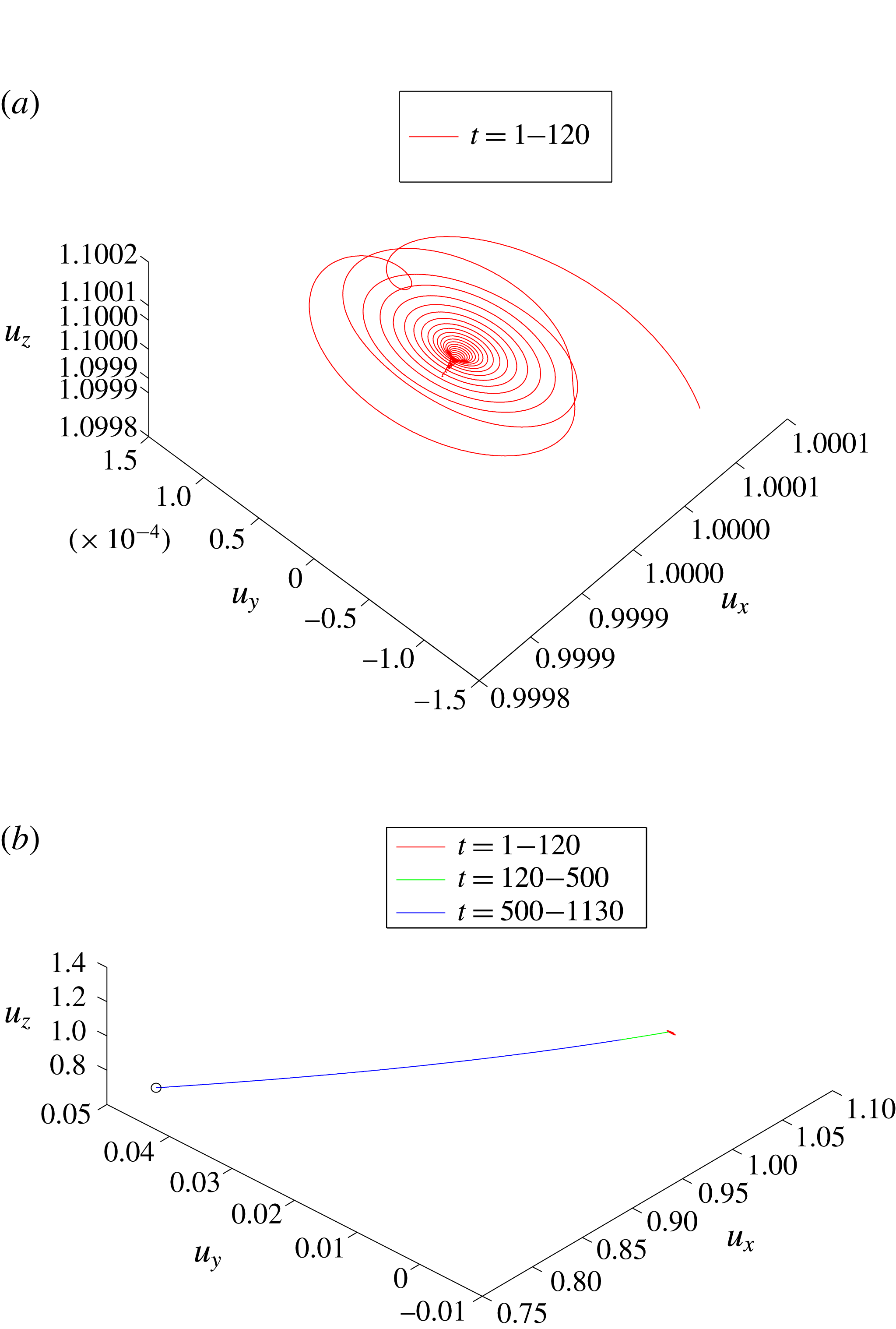
Figure 11(a) shows the velocity trajectory during the time from
 $t=0$
up to
 $t=120$
. Note that the scale of velocity changes during this time period is small,
 $O(10^{-3})$
. The initial flow dynamics consists of two stages of evolution. The first stage is the initial transient stage during
 $0\leqslant t\leqslant 50$
where the trajectory moves towards a linear spiral sink. This describes the decay of all of the stable modes, primarily the
 $m=1$
least stable mode, i.e. the velocity trajectory follows a spiral orbit towards a central point. The second stage is the development of the linear most unstable mode of the base flow starting at
 $t\sim 120$
. The velocity trajectory moves away from the centre of the spiral sink. It continues to evolve along a fixed straight line during the time elapsed from
 $t=120$
to
 $t=500$
, see figure 11(b) and the perturbation shape in figure 10(a) at
 $t=400$
. Note that at this large scale of velocity, the initial transient stage shrinks to almost a point. When
 $t>500$
, the trajectory continues to move along a near straight line (see the perturbation shapes in 10(b) and 10(c)). It asymptotically approaches a stable fixed point of the axisymmetric breakdown state shown in figure 10(d), and stays at this point for all
 $t>1200$
. At the given operational conditions
 $\unicode[STIX]{x1D714}=2.2,~Re=300$
, this stable fixed point of the axisymmetric breakdown state forms an attractor of the flow dynamics.
3.2.2 The case study with
$\unicode[STIX]{x1D714}=2.2,~Re=400$

The growth rate
 $\unicode[STIX]{x1D70E}_{E}$
for the second case with
 $\unicode[STIX]{x1D714}=2.2,~Re=400$
is shown in figure 4. In addition, figure 12 presents snapshots of the streaklines of the flow perturbation at various times from
 $t=400$
to
 $t=1100$
. The flow global evolution in this case may be explained by the following scenario. During the initial time period
 $1<t<50$
, the perturbation exhibits a transition stage where again all of the stable modes of the initial perturbation decay in time. At
 $t$
around
 $50$
, the perturbation takes the form of the most unstable mode of the base flow at
 $\unicode[STIX]{x1D714}=2.2$
and
 $Re=400$
that is also an axisymmetric perturbation mode. During the linear growth stage
 $50<t<350$
this axisymmetric perturbation mode grows in time with a nearly constant growth rate
 $\unicode[STIX]{x1D70E}_{E}=0.0297$
, see figure 12(a). As the perturbation continues to grow in time it eventually forms an axisymmetric separation zone around the pipe centreline. The flow continues to evolve through a saturated nonlinear process during the time period
 $350<t<600$
into a axisymmetric vortex breakdown state at time
 $t=600$
, see the perturbation shape in figure 12(b). However, with further increase of time, an unstable spiral perturbation evolves in the axisymmetric vortex breakdown state, see figure 12(c) at
 $t=645$
. Through a second nonlinear evolution process during the time
 $645<t<1100$
, the axisymmetric breakdown state disappears and the perturbation evolves into a large spiral wave that rotates about the pipe centreline in the same direction of rotation as the base rotating flow, see figure 12(d) at two times
 $t=1099.04$
(red) and
 $t=1100.42$
(black), at approximately
 $180$
degree in phase during the rotation cycle. A three-dimensional, rotating spiral (
 $m=1$
) mode of perturbation dominates the flow for all
 $t>1000$
.
Snapshots of the streaklines consisting of massless particles released at the pipe inlet (
 $x=0$
) on a circle with
 $r=0.05$
for the case
 $\unicode[STIX]{x1D714}=2.2,Re=400$
at: (a)
 $t=400$
, (b)
 $t=600$
, (c)
 $t=645$
, (d)
 $t=1099.04$
(red) and
 $t=1100.42$
(black).

We study the phase portrait of the velocity components
 $(u_{r},u_{\unicode[STIX]{x1D703}},u_{x})$
at the point
 $r=0.5,\unicode[STIX]{x1D703}=0,~x=1.5$
with time
 $t$
, see figure 13. Figure 13(a) shows the velocity trajectory during the time from
 $t=1$
up to
 $t=130$
. The flow dynamics consists of two stages of evolution. The first stage is again the transient stage during
 $1\leqslant t<60$
where the velocity trajectory moves towards a linear spiral sink, which again describes the decay of all stable modes, primarily the
 $m=1$
least stable perturbation mode of the base flow, i.e. the velocity trajectory follows a spiral orbit towards a centre point. The second stage is the development of the linear most unstable mode starting at
 $t\sim 60$
. The velocity trajectory moves away from the centre of the spiral sink along a fixed straight line during the time elapsed from
 $t=60$
to
 $t=130$
. Notice however that the velocity trajectory changes in small scales, of the order of
 $10^{-3}$
. The simulated flow is able to accurately capture the dynamics of this small-scale perturbation.
The phase portrait of
 $(u_{x},u_{y},u_{\unicode[STIX]{x1D703}})|_{(1.5,0.5,0,t)}$
for
 $\unicode[STIX]{x1D714}=2.2$
,
 $Re=400$
. (a)
 $t\in (10,130)$
; the initial transient stage. (b)
 $t\in (1,680)$
; the black straight line is the linear evolution stage. The green near straight line is the saturated nonlinear stage and the trajectory approaches another fixed point. The red line is a spiral source orbit with linear growth rate estimated as
 $\unicode[STIX]{x1D70E}=0.078+i2.0583$
. (c)
 $t\in (1,1100)$
; the green line shows the nonlinear transient stage. (d)
 $t\in (800,1100)$
; the blue line is the orbit approaching to a limit cycle, shown by a closed yellow line.

Figure 13(b) shows the velocity trajectory during the time from
 $t=0$
up to
 $t=680$
on a larger scale. The initial transient stage is too small to be seen at this scale and it shrinks to almost a point. The velocity trajectory moves first along a straight line (the black coloured line) from
 $t=50$
to
 $t=350$
. This represents the exponential linear growth of the velocity components of the axisymmetric perturbation during the linear growth stage,
 $50<t<350$
. This stage is followed by a near-straight-line trajectory till
 $t=600$
. This part corresponds to the nonlinear evolution stage with a decreasing growth of the perturbation. The velocity trajectory approaches a fixed point at
 $t=600$
. This fixed point corresponds to the establishment of the axisymmetric vortex breakdown flow state found at
 $t\sim 600$
, see figure 12(b). However, this fixed point is unstable to a three-dimensional mode of perturbation. The velocity trajectory moves away from this fixed point, following an outward spiral orbit (the red coloured line), which is a typical linear spiral source, see the perturbation shape in figure 12(c). The growth rate of the linear spiral source is estimated from the simulation to be
 $\unicode[STIX]{x1D70E}\sim 0.078+2.0583i$
.
Figure 13(c) shows the complete trajectory for the time from
 $t=0$
to
 $t=1100$
. The green coloured trajectory shows the continuation of the linear spiral source which forms a nonlinear transient stage. The trajectory is eventually attracted to a closed orbit, forming a near-limit-cycle orbit of the rotating spiral breakdown described in figure 12(d). The blue coloured trajectory shows the dense orbit surrounding the limit-cycle orbit (the yellow coloured line). Figure 13(d) shows a closer view of the limit-cycle orbit and the surrounding orbit during the time from
 $t=800$
to
 $t=1100$
. The rotation of the spiral breakdown is estimated to have a frequency of approximately
 $2$
and is in the direction of the base flow rotation. At the given operational conditions
 $\unicode[STIX]{x1D714}=2.2,~Re=400$
and
 $L=2$
, this limit-cycle orbit of the rotating spiral wave breakdown forms an attractor of the flow dynamics.
3.2.3 The case study with
$\unicode[STIX]{x1D714}=2.55,~Re=214$

For the case
 $\unicode[STIX]{x1D714}=2.55,~Re=214$
, figure 14 presents snapshots of the streaklines of the flow. The flow global evolution may be explained by the following scenario, also see the time history of the instantaneous growth rate for this case in figure 6. During the time
 $0<t<9$
, the perturbation exhibits a transition period where all the stable modes of the initial perturbation decay in time. At
 $t$
around
 $9$
the perturbation takes the form of the most unstable mode of the base flow at
 $\unicode[STIX]{x1D714}=2.55,~Re=214,~L=2$
that is a spiral mode. During the linear growth period
 $9<t<170$
this spiral perturbation mode grows in time with a nearly constant growth rate
 $\unicode[STIX]{x1D70E}_{E}=0.036$
. Figure 14(a,b) presents snapshots of streaklines of the growing rotating spiral perturbation at two times,
 $t=139.38$
(red) and
 $t=141.13$
(black), and at two other times,
 $t=179.99$
(red) and
 $t=179.77$
(black), respectively (both at approximately
 $180$
degree in phase during the rotation cycle). As the perturbation continues to grow in time it is stabilized at a saturated nonlinear limit-cycle process when
 $t>290$
and evolves into a large spiral wave with a constant amplitude that rotates about the pipe centreline in the same direction of rotation as the base rotating flow, see figure 14(c) for two snapshots of streaklines of the rotating spiral breakdown at times
 $t=599.69$
(red) and
 $t=601.87$
(black), again, at approximately
 $180$
degree in phase during the rotation cycle. This process of a direct evolution from a spiral instability mode to a spiral breakdown state, without first establishing an axisymmetric breakdown state, was not described before.
The snapshots of the streaklines of the spiral mode perturbation consisting of massless particles released at the pipe inlet (
 $x=0$
) on a circle with
 $r=0.05$
for the case
 $\unicode[STIX]{x1D714}=2.55,~Re=214$
at: (a)
 $t=139.38$
(red) and
 $t=141.13$
(black), (b)
 $t=177.99$
(red) and
 $t=179.77$
(black), (c)
 $t=599.69$
(red) and
 $t=601.87$
(black).

For a low-dimensional representation of the flow dynamics, we again consider the phase portrait of the velocity components
 $(u_{r},~u_{\unicode[STIX]{x1D703}},~u_{x})$
at the point
 $r=0.5,~\unicode[STIX]{x1D703}=0,~x=1.5$
with time
 $t$
. Figure 15 shows various velocity phase portraits up to certain times
 $t$
during the flow evolution from
 $t=1$
to
 $t=600$
.
The phase portrait of
 $(u_{x},u_{y},u_{\unicode[STIX]{x1D703}})|_{(1.5,0.5,0,t)}$
for
 $\unicode[STIX]{x1D714}=2.55$
and
 $Re=214$
. (a)
 $t\in (1,20)$
; the initial transient stage. (b)
 $t\in (1,170)$
. (c)
 $t\in (1,600)$
; linear (red) and nonlinear spiral source (yellow). The trajectory is approaching a limit cycle, shown by a closed black cycle.

Figure 15(a) shows the velocity trajectory at the point
 $r=0.5,\unicode[STIX]{x1D703}=0,~x=1.5$
during the initial stage from
 $t=1$
up to
 $t=20$
. It again consists of two stages of evolution. The first is the transient stage during
 $0\leqslant t\leqslant 9$
where the trajectory moves in a complicated way which describes the decay of all stable modes. The second stage is the development of the linear most unstable mode of the base flow starting at
 $t\sim 9$
. Now the velocity trajectory moves away from the centre of a spiral source along a spiral out orbit (the red coloured line) during time
 $t=9$
to
 $t=20$
. Notice again that the velocity changes occur again at small scales, of the order of
 $10^{-3}$
. The simulated flow correctly captures the dynamics of this fine small-scale perturbation.
Figure 15(b) shows the velocity trajectory from
 $t=1$
to
 $t=170$
on a larger scale. The initial transient stage is too small to be seen in this scale and shrinks to almost a point. The velocity trajectory moves along an outward spiral orbit during the linear growth stage,
 $9<t<170$
, see the perturbation shape in 14(a) and 14(b).
Figure 15(c) shows the complete velocity trajectory during the time period from
 $t=1$
to
 $t=600$
. The trajectory moves for all time along an outward spiral orbit. After the linear stage of the orbit (the red coloured line), the second part of the orbit presents a continued nonlinear saturated process with a decreasing growth of the perturbation size (the yellow coloured line). The velocity trajectory is eventually attracted to a closed limit-cycle orbit (the black coloured line). The rotating spiral breakdown shape for this state is shown in figure 14(d). At the given operational conditions
 $\unicode[STIX]{x1D714}=2.55,~Re=214$
, this limit-cycle orbit of the rotating spiral wave breakdown forms an attractor of the flow dynamics.
4 The attractors of the solid-body rotation flow in a finite-length pipe
The global dynamics of the solid-body rotation flow in a finite-length pipe in response to small initial perturbations is discussed in this section. Two basic approaches have been used in the study of the above representative examples. First, the flow field and perturbation shape (given by streak lines) are described at key times of the flow evolution to determine the flow characteristics. The second approach is based on a low-dimensional representation of the flow dynamics, i.e. the phase portrait in time comprised of the velocity trajectory at a fixed point in the domain. Within the range of
 $Re$
,
 $\unicode[STIX]{x1D714}$
studied in this paper, the combined approaches reveal three basic different scenarios of the perturbed flow evolution:
(i) The first scenario (when
$\unicode[STIX]{x1D714}=2.2$
,
$Re=300$
) is a direct evolution from a linearly unstable axisymmetric disturbance of the base flow to a nonlinear saturated axisymmetric breakdown state, that is a nonlinear modification of the linear instability mode of the base flow.(ii) The second scenario (when
$\unicode[STIX]{x1D714}=2.2$
,
$Re=400$
) is a multistage flow evolution composed of an initial transient stage into a first fixed point, followed by a linear growth stage of an unstable axisymmetric mode of the base flow into an axisymmetric breakdown state (a second fixed point) that is by itself unstable to a secondary spiral mode of perturbation and evolves through a nonlinear spiral source trajectory into a rotating (limit cycle) spiral wave of breakdown of constant amplitude.(iii) The third scenario (when
$\unicode[STIX]{x1D714}=2.55$
,
$Re=214$
) is an evolution composed of an initial transient stage, that is followed by a linear growth stage of an unstable spiral mode, and is continued by a nonlinear spiral source evolution to a large-size saturated rotating (limit cycle) spiral wave of breakdown.


These three scenarios reveal the existence of various types of attractors in the global dynamics of perturbations on the solid-body rotation flow. The flow eventually evolves to a certain attractor that strongly depends on the basin of the attraction in the flow operational map of
 $Re$
versus
 $\unicode[STIX]{x1D714}$
. In the case of
 $\unicode[STIX]{x1D714}=2.2,Re=300$
, the flow is directly attracted by the strong attractor of the axisymmetric breakdown state at these operational conditions. A similar dynamical behaviour is found at other operational points in the range of
 $\unicode[STIX]{x1D714}$
and
 $Re$
that are above but close to the neutral line of the axisymmetric linear mode of the base flow, see the operational conditions with (●) shown in figure 16. In the case of the same
 $\unicode[STIX]{x1D714}=2.2$
with a higher
 $Re$
,
 $Re=400$
, the flow exhibits a different trajectory. It is first attracted by the axisymmetric breakdown state at the given conditions. Then, the flow is further attracted by the strong limit-cycle orbit of a large-amplitude rotating spiral wave, that is an attractor at these operational conditions. A similar dynamical behaviour is found at other operational points above and away from the neutral line of the axisymmetric linear mode of the base flow as well as near the corner point
 $\unicode[STIX]{x1D714}=2.462,Re=263$
of the neutral line, see the operational conditions with (▴) shown in figure 16. The domain of attraction of the axisymmetric breakdown state above the neutral line decreases to zero as the corner point of the neutral line is approached. In the case of a higher
 $\unicode[STIX]{x1D714}$
,
 $\unicode[STIX]{x1D714}=2.55$
with
 $Re=214$
, the flow is directly attracted by the strong limit-cycle orbit of a large rotating spiral perturbation, that is an attractor at these operational conditions. A similar dynamical behaviour is found at all other operational points above the neutral line of the linear
 $m=1$
spiral mode of the base flow, see the operational conditions with (○) shown in figure 16.
Three scenarios of the perturbed flow evolution: the first scenario is a direct evolution from a linearly unstable axisymmetric disturbance of the base flow to a nonlinear saturated axisymmetric breakdown state (∙); the second scenario is composed of a linear growth stage of an unstable axisymmetric mode of the base flow into an axisymmetric breakdown state, followed by an evolution of a secondary unstable spiral mode of perturbation that is eventually saturated on a rotating spiral wave of breakdown (▴); the third scenario is a direct evolution from a linearly unstable spiral disturbance of the base flow to a large-size saturated rotating (limit cycle) spiral wave of breakdown (○). The neutral linear stability line of
 $Re$
versus
 $\unicode[STIX]{x1D714}$
is presented for reference: (dot-dash line:
 $m=0$
axisymmetric mode and solid line is
 $m=1$
spiral mode.

A special case of the present results is the similar scenario of flow evolution revealed first in the flow simulations by Ruith et al. (Reference Ruith, Chen, Meiburg and Maxworthy2003). They found the linear spiral instability mode that initiates an instability of the axisymmetric bubble breakdown state to a dominant attractor describing a large-amplitude, rotating spiral breakdown wave. They claimed that the occurrence of the spiral type of breakdown is induced by an instability of the axisymmetric breakdown state.
In the present study we find that the flow dynamics depends on the operational conditions and is richer in terms of possible scenarios than the scenarios presented in previous papers such as in Wang & Rusak (Reference Wang and Rusak1997), Ruith et al. (Reference Ruith, Chen, Meiburg and Maxworthy2003), Gallaire et al. (Reference Gallaire, Ruith, Meiburg, Chomaz and Huerre2006), Meliga & Gallaire (Reference Meliga and Gallaire2011), where only part of the scenarios were studied. The axisymmetric breakdown evolves directly from an axisymmetric linear instability mode of the base flow, that was first predicted by the Wang & Rusak (Reference Wang and Rusak1996, Reference Wang and Rusak1997) axisymmetric vortex breakdown theory. Depending on
 $\unicode[STIX]{x1D714}$
and
 $Re$
, the spiral type of breakdown can be found from either the secondary instability of an axisymmetric breakdown state but it can also be induced directly by the growth of spiral instability modes of the base flow.
In fact, the present case studies show that the nonlinear dynamics of the flow is a natural extension of the linear dynamics of the base axisymmetric solid-body rotation flow in a finite-length pipe (see Wang & Rusak (Reference Wang and Rusak1996, Reference Wang and Rusak1997), Rusak et al. (Reference Rusak, Wang, Xu and Taylor2012), Rusak & Wang (Reference Rusak and Wang2014) and Wang et al. (Reference Wang, Rusak, Gong and Liu2016)). In particular, it can be observed from figure 16 for the flow with
 $\unicode[STIX]{x1D714}=2.2$
and
 $Re=300$
that is above but close to the linear neutral stability line with
 $m=0$
, that a steady nonlinear saturated state is established as a direct dynamical consequence of the corresponding linear
 $m=0$
instability mode of the base flow. Similarly, the flow with
 $\unicode[STIX]{x1D714}=2.55$
and
 $Re=214$
that is above but close to the linear neutral stability line with
 $m=1$
, shows a nonlinear saturated state of a rotating spiral breakdown wave that is established as a direct dynamical consequence of the corresponding linear
 $m=1$
instability mode of the base flow. Moreover, at certain operational conditions, such as at
 $\unicode[STIX]{x1D714}=2.2$
and
 $Re=400$
, the attractors can interfere one with the other to form several types of attractors and thereby determine a complicated nature of the flow dynamics.
We emphasize that in a real flow apparatus, the various flow set-ups at the pipe inlet (the vortex generator ahead of the pipe) and at the pipe outlet (the discharge device), the pipe geometry (diverging or contracting), the swirl level and Reynolds number can strongly affect the form of an attractor at various operational conditions. The experiments of Sarpkaya (Reference Sarpkaya1971, Reference Sarpkaya1974), Faler & Leibovich (Reference Faler and Leibovich1977) and Garg & Leibovich (Reference Garg and Leibovich1979) already demonstrated the rich dynamics of a swirling flow in a diverging vortex tube with guiding vanes ahead of it. They determined various types of disrupted vortex flows, axisymmetric and spiral breakdown states, and dynamical transitions between them. Also, the numerical flow simulations of Spall & Gatski (Reference Spall and Gatski1991) and Spall (Reference Spall1996) demonstrated the transition from a spiral state of breakdown to an axisymmetric breakdown state and back to a spiral breakdown state. The simulations of Tromp & Beran (Reference Tromp and Beran1997) also described a transition from axisymmetric breakdown state to spiral waves and spiral breakdown states. The current approach that is composed of a linear stability analysis of the base axisymmetric flow together with a low-dimensional representation of the global dynamics deduced from direct numerical simulations can be used in the future to shed further insight on these complicated flow phenomena.
5 Energy transfer mechanism
In this section we follow the analysis of Wang et al. (Reference Wang, Rusak, Gong and Liu2016) of the energy transfer mechanism of three-dimensional perturbations on a base solid-body rotation flow. We first re-derive the Reynolds–Orr equation for the perturbation’s specific integrated kinetic energy
 $E(t)$
, defined by (2.7), see (A 3) in appendix A. Note that (A 3) applies to any size of a perturbation on the base columnar flow and is not limited to small disturbances. Using the computed solution of the perturbation structure as a function of time, as found by the direct numerical simulations based on the Navier–Stokes equations, we then compute the various terms in (A 3) as a function of time
 $t$
. Thereby, we are able to directly assess the contributions of the various sources of production of
 $E(t)$
from inside the bulk and at the boundaries to the instantaneous growth rate
 $\unicode[STIX]{x1D70E}_{E}(t)$
. This provides a direct understanding of the physical mechanism that drives the flow instabilities and the evolution to either axisymmetric or spiral vortex breakdown states without invoking any technical details of stability analysis of the flow.
From the formulation (2.7) and (A 3), we obtain
 $$\begin{eqnarray}\unicode[STIX]{x1D70E}_{E}=\unicode[STIX]{x1D70E}_{E1}+\unicode[STIX]{x1D70E}_{E2}+\unicode[STIX]{x1D70E}_{E3},\end{eqnarray}$$
where
 $$\begin{eqnarray}\displaystyle \unicode[STIX]{x1D70E}_{E1} & = & \displaystyle -{\displaystyle \frac{1}{2\mathscr{E}_{0}}}\int _{S_{2}}u_{x1}p_{1}\,\text{d}S_{2},\end{eqnarray}$$
 $$\begin{eqnarray}\displaystyle \unicode[STIX]{x1D70E}_{E2} & = & \displaystyle -{\displaystyle \frac{1}{2\mathscr{E}_{0}}}{\displaystyle \frac{1}{2}}\int _{S_{2}}u_{x}(u_{r1}^{2}+u_{\unicode[STIX]{x1D703}1}^{2}+u_{x1}^{2})\,\text{d}S_{2}\end{eqnarray}$$
 $$\begin{eqnarray}\displaystyle \unicode[STIX]{x1D70E}_{E3} & = & \displaystyle {\displaystyle \frac{1}{2\mathscr{E}_{0}Re}}\left(-\int _{V_{C}}\left(|\unicode[STIX]{x1D6FB}u_{r1}|^{2}+|\unicode[STIX]{x1D6FB}u_{\unicode[STIX]{x1D703}1}|^{2}+|\unicode[STIX]{x1D6FB}u_{x1}|^{2}\vphantom{{\displaystyle \frac{2u_{r1}}{r^{2}}}}\right.\right.\nonumber\\ \displaystyle & & \displaystyle +\left.{\displaystyle \frac{2u_{r1}}{r^{2}}}{\displaystyle \frac{\unicode[STIX]{x2202}u_{\unicode[STIX]{x1D703}1}}{\unicode[STIX]{x2202}\unicode[STIX]{x1D703}}}+{\displaystyle \frac{u_{r1}^{2}}{r^{2}}}-{\displaystyle \frac{2u_{\unicode[STIX]{x1D703}1}}{r^{2}}}{\displaystyle \frac{\unicode[STIX]{x2202}u_{r1}}{\unicode[STIX]{x2202}\unicode[STIX]{x1D703}}}+{\displaystyle \frac{u_{\unicode[STIX]{x1D703}1}^{2}}{r^{2}}}\right)\text{d}V\nonumber\\ \displaystyle & & \displaystyle \left.+\,\int _{\unicode[STIX]{x2202}V_{C}}\left(u_{r1}{\displaystyle \frac{\unicode[STIX]{x2202}u_{r1}}{\unicode[STIX]{x2202}n}}+u_{\unicode[STIX]{x1D703}1}{\displaystyle \frac{\unicode[STIX]{x2202}u_{\unicode[STIX]{x1D703}1}}{\unicode[STIX]{x2202}n}}+u_{x1}{\displaystyle \frac{\unicode[STIX]{x2202}u_{x1}}{\unicode[STIX]{x2202}n}}\right)\text{d}S\right).\end{eqnarray}$$
 $\unicode[STIX]{x1D70E}_{E1}$
represents the growth rate of the perturbation as a result of the outlet integrated work of the perturbation’s pressure by the perturbation’s axial velocity. The term
 $\unicode[STIX]{x1D70E}_{E2}$
represents the growth rate of the perturbation as a result of the outlet integrated convective loss of perturbation’s kinetic energy by the flow axial velocity. The term
 $\unicode[STIX]{x1D70E}_{E3}$
represents the growth rate of the perturbation as a result of the viscous dissipation of the perturbation’s kinetic energy in the bulk and at the boundaries of the domain. The sum of these three sources determines the perturbation’s instantaneous growth rate in the bulk.
Figure 17 presents the computed values of
 $\unicode[STIX]{x1D70E}_{E1}$
(the solid black line),
 $\unicode[STIX]{x1D70E}_{E2}$
(the solid green line),
 $\unicode[STIX]{x1D70E}_{E3}$
(the solid blue line) and the sum of these three terms,
 $\unicode[STIX]{x1D70E}_{E1}+\unicode[STIX]{x1D70E}_{E2}+\unicode[STIX]{x1D70E}_{E3}$
(the open circles) as a function of
 $t$
for the case
 $\unicode[STIX]{x1D714}=2.55$
,
 $Re=214$
and
 $L=2$
where the base flow is unstable to a rotating spiral mode and evolves to a limit-cycle rotating spiral breakdown. Also shown in figure 17 (the solid red line) is the computed instantaneous growth rate
 $\unicode[STIX]{x1D70E}_{E}(t)$
of the perturbation, taken from figure 6. It can be seen that the line of the sum
 $\unicode[STIX]{x1D70E}_{E1}+\unicode[STIX]{x1D70E}_{E2}+\unicode[STIX]{x1D70E}_{E3}$
nicely matches for all times with the computed line of
 $\unicode[STIX]{x1D70E}_{E}(t)$
. The lines of
 $\unicode[STIX]{x1D70E}_{E1}$
and
 $\unicode[STIX]{x1D70E}_{E2}$
represent the major perturbation kinetic energy production (positive) and loss (negative), respectively. These terms are not directly related to the viscous effect. The viscous effect through
 $\unicode[STIX]{x1D70E}_{E3}$
is negative and causes loss of perturbation kinetic energy for all time. The viscous effect is stabilizing the perturbation and is only slightly dependent on
 $t$
.
The growth rates
 $\unicode[STIX]{x1D70E}_{E1}$
,
 $\unicode[STIX]{x1D70E}_{E2}$
,
 $\unicode[STIX]{x1D70E}_{E3}$
,
 $\unicode[STIX]{x1D70E}_{E1}+\unicode[STIX]{x1D70E}_{E2}+\unicode[STIX]{x1D70E}_{E3}$
and
 $\unicode[STIX]{x1D70E}_{E}$
as a function of
 $t$
for the case
 $\unicode[STIX]{x1D714}=2.55$
,
 $Re=214$
and
 $L=2$
.

During the linear stage of growth of the perturbation,
 $9\leqslant t\leqslant 170$
, the contributions to the instantaneous growth rate from the various components are all nearly constants, as was predicted by the linear stability theory of Wang et al. (Reference Wang, Rusak, Gong and Liu2016). For a fixed
 $Re$
and at inlet swirl levels
 $\unicode[STIX]{x1D714}$
below the neutral line, the perturbation’s pressure work at the outlet is less than the convection of perturbation’s kinetic energy through the outlet and the viscous loss of energy in the bulk and at the boundaries. Then, all perturbation modes of the base flow lose energy and decay in time and the flow is asymptotically stable. However, at inlet swirl levels
 $\unicode[STIX]{x1D714}$
above the neutral line, the instability mode is driven by the perturbation’s pressure work at the outlet with respect to the convection of perturbation’s kinetic energy through the outlet and the viscous loss of energy in the bulk and at the boundaries. The instability modes gain energy from the growing changes at the outlet state. When the perturbation grows to a finite size, the contributions from
 $\unicode[STIX]{x1D70E}_{E1}$
and
 $\unicode[STIX]{x1D70E}_{E2}$
vary in time while
 $\unicode[STIX]{x1D70E}_{E3}$
remains nearly constant in time. We find that
 $\unicode[STIX]{x1D70E}_{E1}$
due to the perturbation’s pressure work at the outlet decreases in size while
 $\unicode[STIX]{x1D70E}_{E2}$
due to the convection of perturbation’s kinetic energy at the outlet increases in negative size between
 $t=170$
and
 $t=240$
. These changes at the outlet form a new balance of the perturbation’s kinetic energy production thereafter, with
 $\unicode[STIX]{x1D70E}_{E}$
approaching zero, i.e. the real part of the growth rate is zero and the perturbation does not grow any longer. The changes of
 $\unicode[STIX]{x1D70E}_{E1}$
and
 $\unicode[STIX]{x1D70E}_{E2}$
stabilize the perturbation on a limit-cycle orbit describing a large-amplitude rotating spiral breakdown for all
 $t>600$
. The variation of
 $\unicode[STIX]{x1D70E}_{E1}$
and
 $\unicode[STIX]{x1D70E}_{E2}$
in time is caused by the significant change of the base flow state by the large-amplitude rotating spiral perturbation.
The energy transfer mechanism during the linear growth stage of the perturbation,
 $9\leqslant t\leqslant 170$
, shows a crucial point; in the physical model of a vortex flow in a finite-length pipe, where the swirling flow is generated by a fixed in place and fixed in time vortex generator ahead of the pipe inlet and the flow discharge device at the outlet is relatively passive, the convective nature of the flow does not allow an inlet–outlet periodicity to occur. The consequence of this periodicity (symmetry) breaking leads to a significant change of the energy transfer mechanism between the perturbation and the base flow and to the loss of stability above a certain swirl ratio. The instability of the solid-body rotation flow in a finite-length pipe is induced by the unbalanced kinetic energy transfer between the perturbation and the base flow. The current study further extends the linear stability result and reveals a nonlinear energy transfer mechanism between the perturbation and base flow that is a natural extension of the linear stability theory. Thus, the onset and the evolution to the vortex breakdown are beyond the reach of the classical vortex stability theory, where an upstream–downstream periodicity is imposed on the flow for all time, but this assumption is not realistic.
Computations of the various sources of perturbation’s kinetic energy production or loss for all other flow simulations described above exhibit a similar behaviour of the way the competition between the various sources determines the fate of the perturbation’s dynamics and the linear and nonlinear stability of the base flow.
6 Mechanism of onset of instability and vortex breakdown
6.1 Local stability versus global stability
It is important to understand further the nature of the instability leading to the vortex breakdown states as arises from the three-dimensional numerical simulations. There has been a considerable effort in the literature to relate the instability of vortex flows to the global stability of a weakly non-parallel developing flow along its main axis in an infinitely long axial domain. This approach relates to the classical absolute/convective instability analysis. In a slightly non-parallel flow governed by a small parameter
 $\unicode[STIX]{x1D716}$
,
 $0<\unicode[STIX]{x1D716}\ll 1$
, a rescaling of the axial length
 $x$
by
 $X=\unicode[STIX]{x1D716}x$
reveals the role of flow stability at various axial cross-sections, and is called local stability analysis. At the dominant order of the problem is the classical stability problem of an axially parallel base flow. The local linear stability properties of the flow at an axial cross-section
 $x$
is determined by the nature of growth of normal mode perturbations on the local flow as a base flow in an infinitely long homogeneous domain. A flow can be classified as locally stable when all perturbations decay in time or absolutely/convectively unstable based on the base flow wave guiding nature, i.e.
(i) Convective instability (CI) occurs when the flow is locally unstable, but, in a fixed laboratory frame, the perturbation diminishes over time.
(ii) Absolute instability (AI) occurs when a flow is locally unstable, but, in a fixed laboratory frame, the perturbation grows in time.
The significance of CI–AI for a spatially weakly developing flow is that such a flow can stay globally linearly stable although it may be characterized locally with a CI. On the other hand, a flow with a sufficient finite region of AI may become a self-sustained wave maker and trigger a global linear instability by a transition from convective to absolute local instability, see for example the pioneering papers by Huerre & Monkewitz (Reference Huerre and Monkewitz1985), Chomaz, Huerre & Lg (Reference Chomaz, Huerre and Redekopp1988) and Huerre & Monkewitz (Reference Huerre and Monkewitz1990).
The CI–AI concept captures the competitive effects of the perturbation’s growth against its convection by the base flow. The underlying physical concept of CI–AI explains that perturbations in a CI region can be amplified but are deemed to convect out of the instability region and that perturbations in an AI region can sustain growth to generate a global mode of instability. We emphasize that the local/global stability (instability) is a closely connected pair of concepts in the stability theory of a weakly non-parallel flow. On the other hand, the various instability processes of the solid-body rotation flow found in the present simulations is of a completely different physical mechanism where the local/global stability (instability) pair does not even exist; the solid-body rotation flow is linearly stable to all normal mode perturbations and is a wave guide (Kelvin Reference Kelvin1880). The instabilities found in this paper are induced by the finite-domain effect, and no local normal mode instability is necessary for the onset of instabilities of the rotating flow in a finite-length pipe.
Moreover, the CI–AI approach is limited in its scope and accuracy of calculations to cases where the base flow is only weakly developing along the axial direction. Moreover, since this approach is based on the local stability properties of the flow profile at various axial cross-sections, it does not allow the full interactions in the flow, i.e. no interaction between the sections properties and the inlet and outlet conditions is described. This may apply to the nature of thin boundary layer or wake flows and of certain regions of vortex flows but not to flows where there may be a strong global interaction between the flow in the bulk and the domain boundaries, including the pipe wall, inlet and outlet. The latter is the case of the stability of a vortex flow in a finite-length domain. In such a case, only a linear stability analysis of the base flow which also includes all the boundary conditions used in the simulations accurately represents the flow dynamics as computed by direct numerical simulations. In the following subsections we further explain this view.
6.2 The study of local/global stability of swirling flows
Ruith et al. (Reference Ruith, Chen, Meiburg and Maxworthy2003) studied the local CI–AI properties of a numerically simulated base axisymmetric and steady vortex breakdown state of a Grabowski–Berger vortex (Grabowski & Berger Reference Grabowski and Berger1976) injected into a semi-infinite domain at
 $Re=200$
and swirl level
 $S=1$
, and that contains a centreline bubble separation zone. They assumed that at any axial cross-section the base flow may be approximated by a Batchelor vortex profile (Batchelor Reference Batchelor1964) with specific parameters of the vortex core size and strength. They used the results of CI–AI analyses of the base Batchelor vortex by Delbende, Chomaz & Huerre (Reference Delbende, Chomaz and Huerre1998) and Olendraru, Sellier & Huerre (Reference Olendraru, Sellier and Huerre1999) to determine the nature of the flow local stability at various axial cross-sections. They found a finite local region of AI that is attached to the rear part of the axisymmetric breakdown bubble and qualitatively attributed this region to the loss of stability of the axisymmetric breakdown state to a certain three-dimensional perturbation and its evolution to a spiral breakdown state. However, they realized that the base flow state has a significant radial expansion around the breakdown bubble and is not a slightly parallel flow state. Therefore, their CI–AI analysis may not lead to any quantitatively accurate and conclusive link between the existence of an absolute instability (AI) region in the axisymmetric breakdown state and the spiral mode of instability of the breakdown bubble.
Realizing the limitations of the CI–AI analysis, and in an attempt to shed additional light on the flow dynamics, Ruith et al. (Reference Ruith, Chen, Meiburg and Maxworthy2003) also developed another strategy to estimate the global instability of the breakdown bubble. They were the first to use three-dimensional direct numerical simulation to describe the shape and growth rate of the rotating spiral mode that destabilizes the bubble and evolves to a spiral breakdown state.
In a follow-up study, Gallaire et al. (Reference Gallaire, Ruith, Meiburg, Chomaz and Huerre2006) further explored the relationship of CI–AI to the global nonlinear mode of instability of the breakdown bubble. They used the base axisymmetric vortex breakdown state computed by Ruith et al. (Reference Ruith, Chen, Meiburg and Maxworthy2003) and assumed that it is a weakly non-parallel base flow. They conducted a thorough linear local stability analysis at all the axial cross-sections of this simulated base flow. According to their CI–AI analysis, they inferred that a nonlinear global mode develops in the axisymmetric breakdown state, triggered by the appearance of a locally absolutely unstable region behind the breakdown bubble. However, the predicted frequency for the dominant
 $m=1$
mode for the case
 $Re=200$
and swirl parameter
 $S=1$
is
 $\unicode[STIX]{x1D70E}_{i}\sim 1.3$
, which is higher than the frequency of the dominant mode found in the simulation of Ruith et al. (Reference Ruith, Chen, Meiburg and Maxworthy2003) where
 $\unicode[STIX]{x1D70E}_{i}=1.18$
. More seriously, their study showed that the transition from CI to AI for the
 $m=1$
mode first occurs at the axial location near the nose of the breakdown bubble where the base flow exhibits a significant radial expansion, as shown by their non-parallelism parameter in figure 2 of Gallaire et al. (Reference Gallaire, Ruith, Meiburg, Chomaz and Huerre2006). Thus, the weakly non-parallel flow assumption of the base flow is not justified. Moreover, they also do not show any evidence that the predicted shape of the absolutely unstable mode indeed becomes a wave maker and is similar to the shape of the linear growth mode of global instability simulated by Ruith et al. (Reference Ruith, Chen, Meiburg and Maxworthy2003). This invalidation can be clearly observed by the reported absolutely unstable wavelength of
 $\unicode[STIX]{x1D706}_{0}=13.1$
, which is far greater than any length scale of the AI region and cannot be considered as a slightly non-parallel flow. The authors claimed, however, that this length scale found from the CI–AI analysis is consistent with the Ruith et al. (Reference Ruith, Chen, Meiburg and Maxworthy2003) simulation result for the spiral mode, but this is an ad hoc conclusion drawn with no direct correlation between the CI–AI results and the simulation results. In conclusion, they did not establish a sufficient convincing evidence that CI–AI analysis can indeed induce the global spiral instability of the breakdown bubble.
6.3 A vortex stability approach based on real physical boundary conditions
We refer again to the study of Ruith et al. (Reference Ruith, Chen, Meiburg and Maxworthy2003) who deduced the linear stability characteristics of the destabilizing spiral mode of the axisymmetric breakdown state directly from results of direct numerical simulation of flow evolution. This led them for the first time to the discovery of a clean linearly unstable spiral mode that is responsible for a spiral type of vortex breakdown. The specific growth rates and frequencies of the unstable spiral mode quantitatively identified by their study became the benchmark for further study. For the case
 $Re=200$
and
 $S=1$
, the
 $m=1$
mode is the most unstable perturbation and is characterized by a complex growth rate,
 $\unicode[STIX]{x1D70E}=0.0359+1.18i$
. The mode shape of the linear eigenmode has a typical wavenumber of approximately
 $k=1/5$
, evidently not supporting the weakly non-parallel assumption in the local/global stability relationship. Moreover, the unstable mode (presented in figure 30 of Ruith et al. (Reference Ruith, Chen, Meiburg and Maxworthy2003) shows a spatial development in the axial direction and the corresponding mode shape is spiral (not helical). This mode is formed by the strong interaction of the vortex flow in the bulk and the imposed physical constraints at the inlet (upstream state) where the velocity profiles are fixed, at the radial far field and at the downstream. The eigenmode obtained does not show a correlation to the CI–AI transition location described by the analysis of Gallaire et al. (Reference Gallaire, Ruith, Meiburg, Chomaz and Huerre2006).
The finding of the linearly unstable spiral modes of Ruith et al. (Reference Ruith, Chen, Meiburg and Maxworthy2003) is an important contribution to the vortex stability theory. It clarifies the nature of the linear mode. This study raised the issue of the importance of quantitative evidence in supporting a theory. This is particularly important as highly accurate computation is available and thus quantitative evidence must be established for testing of a theory. Along this line, in a recent study, Meliga & Gallaire (Reference Meliga and Gallaire2011) performed a linear stability analysis of the base axisymmetric vortex breakdown state obtained by Ruith et al. (Reference Ruith, Chen, Meiburg and Maxworthy2003) where they used the same boundary conditions of Ruith et al. (Reference Ruith, Chen, Meiburg and Maxworthy2003). They confirmed with high accuracy the benchmark linear stability results obtained originally by Ruith et al. (Reference Ruith, Chen, Meiburg and Maxworthy2003). For example, for the case
 $Re=200$
and
 $S=1$
they found that the
 $m=1$
mode is the most unstable mode with growth rate
 $\unicode[STIX]{x1D70E}=0.0387+1.16i$
, which is close to the benchmark result, especially the frequency has three digits accuracy. Moreover, the corresponding mode shape presented in their study is sufficiently close to the one found in Ruith et al. (Reference Ruith, Chen, Meiburg and Maxworthy2003). This shows that only when the same boundary conditions are used in the linear stability analysis as in the simulation, can an accurate prediction of the spiral mode of instability of the breakdown bubble be found. It should be pointed out that the study of Meliga & Gallaire (Reference Meliga and Gallaire2011) is essentially in the same spirit as the analysis of Wang & Rusak (Reference Wang and Rusak1996), where realistic constraints on the vortex flow were used. The instability is, therefore, induced by the strong influence of the imposed physical conditions, which effectively eliminate the weakly non-parallel nature of the base flow. Such an accurate result cannot be obtained by CI–AI analysis since the crucial boundary conditions are ignored in this approach.
6.4 The strong non-parallel flow effect on vortex stability
The significance of the current study is that the selected nominal base flow, solid-body rotation flow with a uniform axial velocity, is the only strain-free flow. Therefore, it exhibits very special stability characteristics, i.e. lack of any instability mechanism including transient growth within the framework of classical normal mode analysis (Kelvin Reference Kelvin1880). This is equally true for any type of perturbation, axisymmetric (
 $m=0$
) or helical (
 $m\neq 0$
). Thus, CI–AI is completely unrelated to the instability mechanism of the solid-body rotation flow in a finite-length pipe found in the present simulations. This is the reason we conducted in § 5 the analysis of energy transfer mechanism based on the Reynolds–Orr equation. This analysis clearly demonstrates that the instability mechanism, discovered originally by Wang & Rusak (Reference Wang and Rusak1996) and followed by Wang et al. (Reference Wang, Rusak, Gong and Liu2016) and by the present study, is essentially a new flow instability mechanism, beyond the scope of classical normal mode analysis, i.e. it is a finite-length domain instability. As shown in the present study, this new ingredient of flow stability is the only mechanism that leads to the onset of the various types of vortex breakdown in a solid-body rotation flow in a finite-length pipe.
The current study also consolidates the view that the instability arising from the unstable spiral mode of Ruith et al. (Reference Ruith, Chen, Meiburg and Maxworthy2003) is also a finite-length domain instability and is beyond the scope of the classical flow instability based on the normal mode or CI–AI analyses. To further illustrate this idea, we conducted an energy analysis based on the Reynolds–Orr equation (A 1) where in this case the base flow is the axisymmetric breakdown state established by a special axisymmetric simulation at
 $\unicode[STIX]{x1D714}=2.2$
and
 $Re=400$
with the same boundary conditions stated in § 2. We computed the linear spiral mode of instability perturbation that evolves in this base flow state and that stabilizes over time on the rotating spiral vortex breakdown state as described in § 3.2.2. We computed for this linear mode of instability the various production (loss) terms of the perturbation’s kinetic energy in the right-hand side of (A 1). We first note from the inlet conditions that the second and fourth terms on the right-hand side of (A 1) vanish. Figure 18(a) shows (dash line) the axial distribution of the integrated energy production at cross-sections
 $x$
in the bulk between the inlet and the outlet as found from the inviscid effect (the axial distribution of the radially integrated integrand in the first term in (A 1)). Also shown is the axial distribution of the viscous damping effect in the bulk (dash-dot line, from the sixth term in (A 1)). The sum of these two bulk effects is also shown (solid line). We note that the seventh term of the viscous effects is very small. It is clear that the overall perturbation’s kinetic production in the bulk (the integrated combined effects due the sum of the two terms) is negative and contributes an integrated negative growth rate of the perturbations kinetic energy in the amount of
 $\unicode[STIX]{x1D70E}_{E,internal}\sim -0.097$
. If the base flow was weakly non-parallel and the AI mechanism was the major source for the onset of the linear spiral mode of instability in the axisymmetric breakdown state, then this integrated combination of effects in the bulk should have been positive and not negative. This rules out the relationship between AI and the mode instability of the axisymmetric breakdown state.
Moreover, we find that the main energy production from the third and fifth terms of right-hand side of (A 1) comes from the outlet state as shown by figure 18(b). It can be seen that the radial distribution of the work performed at the outlet by the pressure perturbation on the axial velocity perturbation (the dash-dot line) overcomes for all
 $r$
the radial distribution of the convective perturbation’s kinetic energy loss at the outlet (dash line). The combined radial distribution of effects at the outlet (the solid line) is positive all across the outlet section from the centreline to the wall. This combined effect contributes an integrated positive growth rate of perturbation kinetic energy production at the outlet where
 $\unicode[STIX]{x1D70E}_{E,outlet}=+0.174$
. The net effect from the bulk and the outlet produces a growth rate of the linear spiral mode of perturbation that is
 $\unicode[STIX]{x1D70E}_{E}=\unicode[STIX]{x1D70E}_{E,outlet}+\unicode[STIX]{x1D70E}_{E,internal}\sim 0.077$
. The use of the Reynolds–Orr equation gives a growth rate of the spiral instability mode in the axisymmetric breakdown state that is similar to that found in the simulation, where
 $\unicode[STIX]{x1D70E}_{E}\sim 0.078$
. It shows that this instability is caused by the axial flow inhomogeneity in the strong non-parallel base flow and is driven by the imbalance between the base flow in the bulk, the inlet state and the outlet state.
The various production (loss) terms of the perturbation’s kinetic energy: (a) distribution along the pipe axis inside of the bulk, and (b) at the outlet.

We also present figure 19, which shows the spatial distribution of the production of an inviscid perturbation’s kinetic energy in the bulk (
 $0\leqslant x\leqslant 2$
and
 $0\leqslant r\leqslant 1$
) as computed from the integrand of the first term on the right-hand side of (A 1). We can see that there is a significant loss of energy along the pipe, specifically around
 $x=1.4$
and
 $r=0.25$
, and production of energy near the outlet at
 $r\sim 0.55$
. The energy pattern has a nearly one wavelength distribution and this cannot be described by a weakly non-parallel assumption about the flow used in CI–AI analyses. The figure actually demonstrates the strong non-parallel flow effect on the perturbation mode that is induced by the boundary conditions which form the axial inhomogeneity in the flow. This is further evidence that the instability mode cannot be driven by an CI–AI mechanism.
The inviscid perturbation’s kinetic energy productions’ density inside of the domain.

In the case of a general vortex flow in a finite-length domain, the Reynolds–Orr equation shows that the instability is caused essentially by the non-axial homogeneity of the base flow and the imbalance of the exchange of the perturbation’s kinetic energy between the base flow in the bulk (except the solid-body rotation flow) and the boundary settings at the domain inlet and outlet. Note that the non-axial homogeneity is also an element in a weakly non-parallel flow approach but it has a completely different role in the instability onset.
In the local/global stability pair, the instability is caused by a sufficiently strong AI region to sustain the perturbation’s growth. Actually, a weak non-parallel flow inhomogeneity by itself modulates the wave but is not the cause of instability. The instability in such an approach depends on the local sectional instability nature as found from normal mode analysis. In a sharp contrast to that, a strong non-parallel flow inhomogeneity induces instability by itself as found in the present study for the solid-body rotation flow in a finite-length pipe. This is made even more striking since in the current study the finite domain is a pipe with an axial length scale that is the same as the diameter of pipe. In such a case the weakly non-parallel flow assumption has no value. Extending the present analysis to other base flows such as the Lamb–Oseen vortex (Gong Reference Gong2017) or the a Grabowski–Berger vortex (Ruith et al. Reference Ruith, Chen, Meiburg and Maxworthy2003) shows a similar dynamical behaviour where the underlying instability mechanism remains the same. We therefore conjecture that the instability found in the current simulations is a general vortex stability behaviour for a confined vortex flow with sufficient swirl. The root cause of this instability was first revealed by the Wang & Rusak (Reference Wang and Rusak1996) analysis and is clearly explained by the use of the Reynolds–Orr equation as a diagnostic tool of the simulation results. An alternative approach is to use the direct numerical simulation to identify the instability process, as was first done by Ruith et al. (Reference Ruith, Chen, Meiburg and Maxworthy2003), in tandem with analysis based on the Reynolds–Orr equation.
6.5 The role of instability in the onset of vortex breakdown
This study provides strong quantitative evidence to support the stability results and the onset mechanism of various types of vortex breakdown and answers the crucial question as to how the vortex breakdown process starts and evolves into various types of breakdown states. The main results shown in figures 8, 16 and 17 demonstrate the consistency of the direct numerical simulation results with the linear stability theories of Wang & Rusak (Reference Wang and Rusak1996) and of Wang et al. (Reference Wang, Rusak, Gong and Liu2016). These include:
(i) The simulated flows strictly obey the predicted swirling flow dynamics found in the linear stability analysis when the perturbation is sufficiently small and thereby clarify the physical conditions
$Re$
versus
$\unicode[STIX]{x1D714}$
for the onset of instabilities and the vortex breakdown process.(ii) The simulated nonlinear dynamics of the flow can be understood by instantaneous flow snapshots and the related phase portraits of the velocity trajectory at a point in the domain. This provides a clear explanation of the various flow evolution paths, the forms of vortex breakdown states and the possible transitions among them.
(iii) The analysis of the energy transfer mechanism reveals an essential ingredient of the physical mechanism that drives the linear as well as the nonlinear flow dynamics, i.e. the loss of flow axial homogeneity between the inlet and outlet by the flow convective nature, and the associated competition between energy production or loss inside the bulk and at the boundaries.


These findings provide an integrated dynamical picture for the onset of the vortex breakdown process and evolution to various breakdown states on the solid-body rotation flow in a finite-length pipe. They also provide a consistent and unified theoretical explanation of the vortex breakdown phenomenon, axisymmetric or spiral, in a solid-body rotation flow in a finite-length pipe. In particular, we point out that the onset of the process of vortex breakdown in a solid-body rotation flow is not related to Benjamin’s vortex breakdown theory, where the axisymmetric vortex breakdown is interpreted as a result of a supercritical–subcritical jump transition analogous to the hydraulic jump phenomenon. The flow transition in vortex breakdown is essentially smooth and neither a super–sub critical transition nor a hydraulic jump phenomenon are found in the simulation.
We shall emphasize that the solid-body rotation flow is closely related to other flow models. The result can be used for large core size of Lamb–Ossen vortices (a family of Batchelor vortex) and can also be readily extended by computational efforts to other vortex flow models including the Batchelor vortex. More importantly the fundamental mechanism revealed by this study evidently has a general nature in regard to the understanding of the vortex breakdown phenomenon in various flow configurations.
7 Conclusions
This paper uses direct numerical simulations to study the dynamics of three-dimensional, incompressible and viscous flows of a base solid-body rotation flow with a uniform axial velocity entering a rotating, finite-length, straight circular pipe. The simulations provide the base flow neutral stability line in response to either axisymmetric or three-dimensional perturbations in a
 $Re$
versus
 $\unicode[STIX]{x1D714}$
operational diagram (figure 8). This line is in good agreement with the neutral stability line predicted by the linear stability theory of Wang et al. (Reference Wang, Rusak, Gong and Liu2016). This agreement supports the accuracy of the simulations in predicting the initial growth of dominant small perturbations on the base flow while supporting the theoretical stability predictions.
Global analysis tools are applied to understand the global dynamics of the flow. We construct a three-dimensional phase portrait composed of the trajectory in time of the three velocity components at a certain point in the flow. These phase portraits provide a low-dimensional representation of the flow dynamics. The phase portraits capture the main flow global nonlinear dynamics and its long-term behaviour. Depending on the operational conditions, these portraits show the existence of stable and unstable focus states as well as saturated limit-cycle orbits during the flow evolution. The use of these portraits helps to identify the various stages of the flow evolution and provides domains of attraction in the operational diagram in figure 16 for various long-term states. The simulated flow evolution can be also analysed via the Reynolds–Orr equation to explore the mechanism that governs the perturbations dynamics (§ 5).
The simulation results demonstrate the various possible scenarios of the global evolution of perturbations and transition phenomena between bubble and spiral breakdown states, as summarized in figure 16. These include: (i) at
 $2.1<\unicode[STIX]{x1D714}<2.45$
and
 $Re$
close to the neutral line, the growth in time of a small disturbance axisymmetric instability mode to form an axisymmetric breakdown state that is a strong attractor state, as predicted by Wang & Rusak (Reference Wang and Rusak1996, Reference Wang and Rusak1997); (ii) at
 $2.1<\unicode[STIX]{x1D714}<2.45$
and higher
 $Re$
above the neutral line, the growth of a small disturbance axisymmetric instability mode, predicted by Wang & Rusak (Reference Wang and Rusak1996), to form an axisymmetric breakdown state that is by itself unstable to a three-dimensional instability mode and evolves to a strong attractor, rotating spiral breakdown wave; and (iii) at higher
 $\unicode[STIX]{x1D714}$
in the range of
 $2.45<\unicode[STIX]{x1D714}<2.6$
, the growth of a small disturbance spiral instability mode, predicted by Wang et al. (Reference Wang, Rusak, Gong and Liu2016), to form a strong attractor, spiral breakdown state.
The analysis based on the Reynolds–Orr equation reveals the mechanism that drives all the instability modes as well as the nonlinear global flow evolution. At high swirl ratios
 $\unicode[STIX]{x1D714}>2.1$
, the confined kinetic energy in a swirling flow in a finite domain can be triggered to be released through various physical agents, such as the non-periodic (asymmetric) conditions set at the pipe inlet and outlet. Other agents may include the viscous effects and pipe geometry changes. These agents eliminate the axial homogeneity along the pipe and thereby induce flow instabilities. They also govern the long-term evolution of the growing perturbations to the various saturated breakdown states, including the transition from axisymmetric breakdown states to spiral breakdown states. This crucial mechanism has been substantiated by the present conclusive analysis. It also sheds new light on the previous three-dimensional flow simulations of Spall & Gatski (Reference Spall and Gatski1991), Spall (Reference Spall1996), Cary et al. (Reference Cary, Darmofal and Powell1997), Tromp & Beran (Reference Tromp and Beran1997) and Ruith et al. (Reference Ruith, Chen, Meiburg and Maxworthy2003).
The discussion in § 6 shows that local instability or its extension using the assumption of a weakly non-parallel flow to conduct CI–AI analysis is definitely not related to any of the instability modes found in the present study. Moreover, a stability study based on the strongly non-parallel flow character, including the axial inhomogeneity due to a finite-domain boundary conditions, must be conducted to determine flow instabilities in such complicated flows. The instabilities may be computed by simulation (as was done in Ruith et al. (Reference Ruith, Chen, Meiburg and Maxworthy2003)) or using linear stability analysis with all applicable boundary conditions. Both computations can supported by an energy analysis based on the Reynolds–Orr equation to determine interaction effects between the flow in the bulk and the flow at the domain boundaries.
Appendix. The Reynolds–Orr equation
For an axisymmetric base flow with velocity components,
 $\boldsymbol{u}_{0}=(u_{0x},u_{0r},u_{0\unicode[STIX]{x1D703}})$
, the Reynolds–Orr equation (see, for example, Serrin Reference Serrin1959) relates the rate of change in time of
 $E$
to various source terms. The Reynolds–Orr equation in the cylindrical coordinates reads
 $$\begin{eqnarray}\displaystyle & & \displaystyle {\displaystyle \frac{\text{d}E(t)}{\text{d}t}}=-\int _{V_{C}}(u_{r1},u_{\unicode[STIX]{x1D703}1},u_{x1})\unicode[STIX]{x1D63D}(u_{r1},u_{\unicode[STIX]{x1D703}1},u_{x1})^{\text{T}}\,\text{d}V+\int _{S_{1}}u_{x1}p_{1}\,\text{d}S_{1}-\int _{S_{2}}u_{x1}p_{1}\,\text{d}S_{2}\nonumber\\ \displaystyle & & \displaystyle \quad +\,{\displaystyle \frac{1}{2}}\int _{S_{1}}u_{x}(u_{r1}^{2}+u_{\unicode[STIX]{x1D703}1}^{2}+u_{x1}^{2})\,\text{d}S_{1}-{\displaystyle \frac{1}{2}}\int _{S_{2}}u_{x}(u_{r1}^{2}+u_{\unicode[STIX]{x1D703}1}^{2}+u_{x1}^{2})\,\text{d}S_{2}\nonumber\\ \displaystyle & & \displaystyle \quad -\,{\displaystyle \frac{1}{Re}}\int _{V_{C}}\!\left(|\unicode[STIX]{x1D6FB}u_{r1}|^{2}+|\unicode[STIX]{x1D6FB}u_{\unicode[STIX]{x1D703}1}|^{2}+|\unicode[STIX]{x1D6FB}u_{x1}|^{2}+{\displaystyle \frac{2u_{r1}}{r^{2}}}{\displaystyle \frac{\unicode[STIX]{x2202}u_{\unicode[STIX]{x1D703}1}}{\unicode[STIX]{x2202}\unicode[STIX]{x1D703}}}+{\displaystyle \frac{u_{r1}^{2}}{r^{2}}}-{\displaystyle \frac{2u_{\unicode[STIX]{x1D703}1}}{r^{2}}}{\displaystyle \frac{\unicode[STIX]{x2202}u_{r1}}{\unicode[STIX]{x2202}\unicode[STIX]{x1D703}}}+{\displaystyle \frac{u_{\unicode[STIX]{x1D703}1}^{2}}{r^{2}}}\right)\text{d}V\nonumber\\ \displaystyle & & \displaystyle \quad +\,{\displaystyle \frac{1}{Re}}\int _{\unicode[STIX]{x2202}V_{C}}\left(u_{r1}{\displaystyle \frac{\unicode[STIX]{x2202}u_{r1}}{\unicode[STIX]{x2202}n}}+u_{\unicode[STIX]{x1D703}1}{\displaystyle \frac{\unicode[STIX]{x2202}u_{\unicode[STIX]{x1D703}1}}{\unicode[STIX]{x2202}n}}+u_{x1}{\displaystyle \frac{\unicode[STIX]{x2202}u_{x1}}{\unicode[STIX]{x2202}n}}\right)\,\text{d}S.\end{eqnarray}$$
Here
 $S_{1}$
and
 $S_{2}$
are the pipe inlet and outlet sections, respectively; the boundary
 $\unicode[STIX]{x2202}V_{C}$
is the domain’s control surface (the inlet, outlet and wall);
 $\unicode[STIX]{x2202}/\unicode[STIX]{x2202}n$
is the directional derivative in the outer normal direction of
 $\unicode[STIX]{x2202}V_{C}$
. Also,
 $\unicode[STIX]{x1D63D}$
is the symmetric strain-rate tensor of the base flow, given in cylindrical coordinates by
 $$\begin{eqnarray}\displaystyle \unicode[STIX]{x1D63D}={\displaystyle \frac{1}{2}}\left[\begin{array}{@{}ccc@{}}2{\displaystyle \frac{\unicode[STIX]{x2202}u_{0r}}{\unicode[STIX]{x2202}r}} & r{\displaystyle \frac{\unicode[STIX]{x2202}}{\unicode[STIX]{x2202}r}}\left({\displaystyle \frac{u_{0\unicode[STIX]{x1D703}}}{r}}\right) & {\displaystyle \frac{\unicode[STIX]{x2202}u_{0x}}{\unicode[STIX]{x2202}r}}+{\displaystyle \frac{\unicode[STIX]{x2202}u_{0r}}{\unicode[STIX]{x2202}x}}\\ r{\displaystyle \frac{\unicode[STIX]{x2202}}{\unicode[STIX]{x2202}r}}\left({\displaystyle \frac{u_{0\unicode[STIX]{x1D703}}}{r}}\right) & {\displaystyle \frac{2u_{0r}}{r}} & {\displaystyle \frac{\unicode[STIX]{x2202}u_{0\unicode[STIX]{x1D703}}}{\unicode[STIX]{x2202}x}}\\ {\displaystyle \frac{\unicode[STIX]{x2202}u_{0x}}{\unicode[STIX]{x2202}r}}+{\displaystyle \frac{\unicode[STIX]{x2202}u_{0r}}{\unicode[STIX]{x2202}x}} & {\displaystyle \frac{\unicode[STIX]{x2202}u_{0\unicode[STIX]{x1D703}}}{\unicode[STIX]{x2202}x}} & 2{\displaystyle \frac{\unicode[STIX]{x2202}u_{0x}}{\unicode[STIX]{x2202}x}}\end{array}\right]. & & \displaystyle\end{eqnarray}$$
We emphasize that the Reynolds–Orr equation applies to any type (axisymmetric or three-dimensional) and to any size of perturbation and therefore demonstrates the nonlinear kinetic energy exchange between the base flow and the perturbation to determine the fate of the perturbation.
For a base columnar solid-body rotation flow with a uniform axial velocity,
 $u_{0x}=1$
,
 $u_{0r}=0$
and
 $u_{0\unicode[STIX]{x1D703}}=\unicode[STIX]{x1D714}r$
, and the symmetric strain-rate tensor
 $\unicode[STIX]{x1D63D}$
vanishes in the entire flow domain. Therefore, the first integral on the right-hand side of (A 1) vanishes. In addition, the two integrals over the inlet surface
 $S_{1}$
also vanish due to the no velocity perturbation conditions at the inlet. As a result, the rate of change of the perturbation’s kinetic energy
 $E$
in time is given for all
 $t>0$
by,
 $$\begin{eqnarray}\displaystyle & & \displaystyle {\displaystyle \frac{\text{d}E(t)}{\text{d}t}}=-\int _{S_{2}}u_{x1}p_{1}\,\text{d}S_{2}-{\displaystyle \frac{1}{2}}\int _{S_{2}}u_{x}(u_{r1}^{2}+u_{\unicode[STIX]{x1D703}1}^{2}+u_{x1}^{2})\,\text{d}S_{2}\nonumber\\ \displaystyle & & \displaystyle \quad -\,{\displaystyle \frac{1}{Re}}\int _{V_{C}}\!\left(|\unicode[STIX]{x1D6FB}u_{r1}|^{2}+|\unicode[STIX]{x1D6FB}u_{\unicode[STIX]{x1D703}1}|^{2}+|\unicode[STIX]{x1D6FB}u_{x1}|^{2}+{\displaystyle \frac{2u_{r1}}{r^{2}}}{\displaystyle \frac{\unicode[STIX]{x2202}u_{\unicode[STIX]{x1D703}1}}{\unicode[STIX]{x2202}\unicode[STIX]{x1D703}}}+{\displaystyle \frac{u_{r1}^{2}}{r^{2}}}-{\displaystyle \frac{2u_{\unicode[STIX]{x1D703}1}}{r^{2}}}{\displaystyle \frac{\unicode[STIX]{x2202}u_{r1}}{\unicode[STIX]{x2202}\unicode[STIX]{x1D703}}}+{\displaystyle \frac{u_{\unicode[STIX]{x1D703}1}^{2}}{r^{2}}}\right)\text{d}V\nonumber\\ \displaystyle & & \displaystyle \quad +\,{\displaystyle \frac{1}{Re}}\int _{\unicode[STIX]{x2202}V_{C}}\left(u_{r1}{\displaystyle \frac{\unicode[STIX]{x2202}u_{r1}}{\unicode[STIX]{x2202}n}}+u_{\unicode[STIX]{x1D703}1}{\displaystyle \frac{\unicode[STIX]{x2202}u_{\unicode[STIX]{x1D703}1}}{\unicode[STIX]{x2202}n}}+u_{x1}{\displaystyle \frac{\unicode[STIX]{x2202}u_{x1}}{\unicode[STIX]{x2202}n}}\right)\text{d}S.\end{eqnarray}$$
The first term on the right-hand side of (A 3) represents the work done by the pressure perturbation due to the axial velocity perturbation at the outlet. This term cannot be computed without a solution of the flow perturbation.



