1 Introduction
Hypersonic laminar–turbulent transition is very complex and is still a major unresolved topic in fluid dynamics. The understanding of high-speed boundary-layer transition is required in order to develop reliable transition prediction methods that can be used for the design and safe operation of advanced high-speed vehicles. Transition to turbulence in supersonic/hypersonic boundary layers is associated with considerable increases in heat transfer. The increased heat loads on the structure of hypersonic vehicles represent one of the main difficulties in designing and operating such vehicles. Appropriate measures to guard against the heat transfer due to aero-thermal loads are expensive and/or result in significant weight penalties. Reliable estimates of the transition location are of vital importance because only then can the aero-thermal loads and surface temperatures be adequately predicted. In addition to surface heating, transition to turbulence also has a significant effect on the aerodynamic performance of high-speed flight vehicles, as the skin friction for turbulent boundary layers is considerably higher than for the laminar boundary layer.
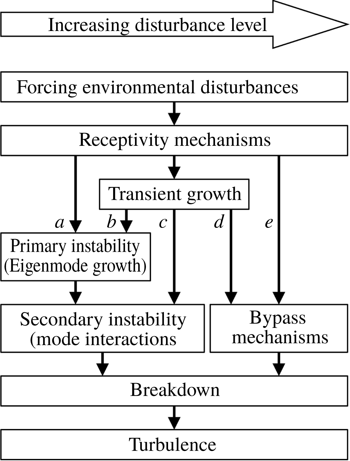
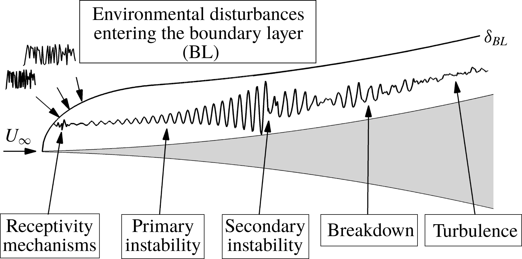
Laminar–turbulent transition in high-speed boundary layers can take various paths, as outlined by Morkovin (Reference Morkovin and Wells1969) (see figure 1). Along which route transition occurs depends largely on the free-stream disturbance level. For quiet tunnel conditions with a low level of free-stream turbulence, such as for the Boeing/AFOSR Mach 6 Quiet Tunnel (BAM6QT) at Purdue University, the stages of the transition process from the natural disturbance environment all the way to turbulence (path a in figure 1) are schematically shown in figure 2. The vital role of quiet tunnels in combination with numerical studies in understanding hypersonic transition and to develop physics based transition prediction methods is discussed by Schneider (Reference Schneider2015).
Paths to transition (adapted from Morkovin Reference Morkovin and Wells1969).

Schematic of the different regions of path a (drawing not to scale).

Experiments carried out by Kimmel (Reference Kimmel1993) and Kimmel, Poggie & Schmisseur (Reference Kimmel, Poggie and Schmisseur2000) at the Arnold Engineering Development Center (AEDC) Tunnel B for a nominal Mach number of 7.93 showed that an adverse pressure gradient generated by a cone flare accelerates transition. The flared cone model in this experimental campaign consisted of a 0.483 m long conical fore-body with a
 $7^{\circ }$
half-angle, a nominal nose radius of
 $5\times 10^{-5}~\text{m}$
and a flared after-body of 0.5334 m length. The cone flare was designed based on a modified Newtonian hypersonic flow theory to achieve constant pressure gradients along the flared after-body (see Shope Reference Shope1991).
Lachowicz, Chokani & Wilkinson (Reference Lachowicz, Chokani and Wilkinson1996a
,Reference Lachowicz, Chokani and Wilkinson
b
) used a flared cone to induce transition on the model within the quiet flow region of the NASA Langley Mach 6 Nozzle Test Chamber Facility (M6NTC) for
 $Re_{1}\approx 0.86\times 10^{6}~\text{m}^{-1}$
. The flared cone geometry used in these studies consisted of a
 $5^{\circ }$
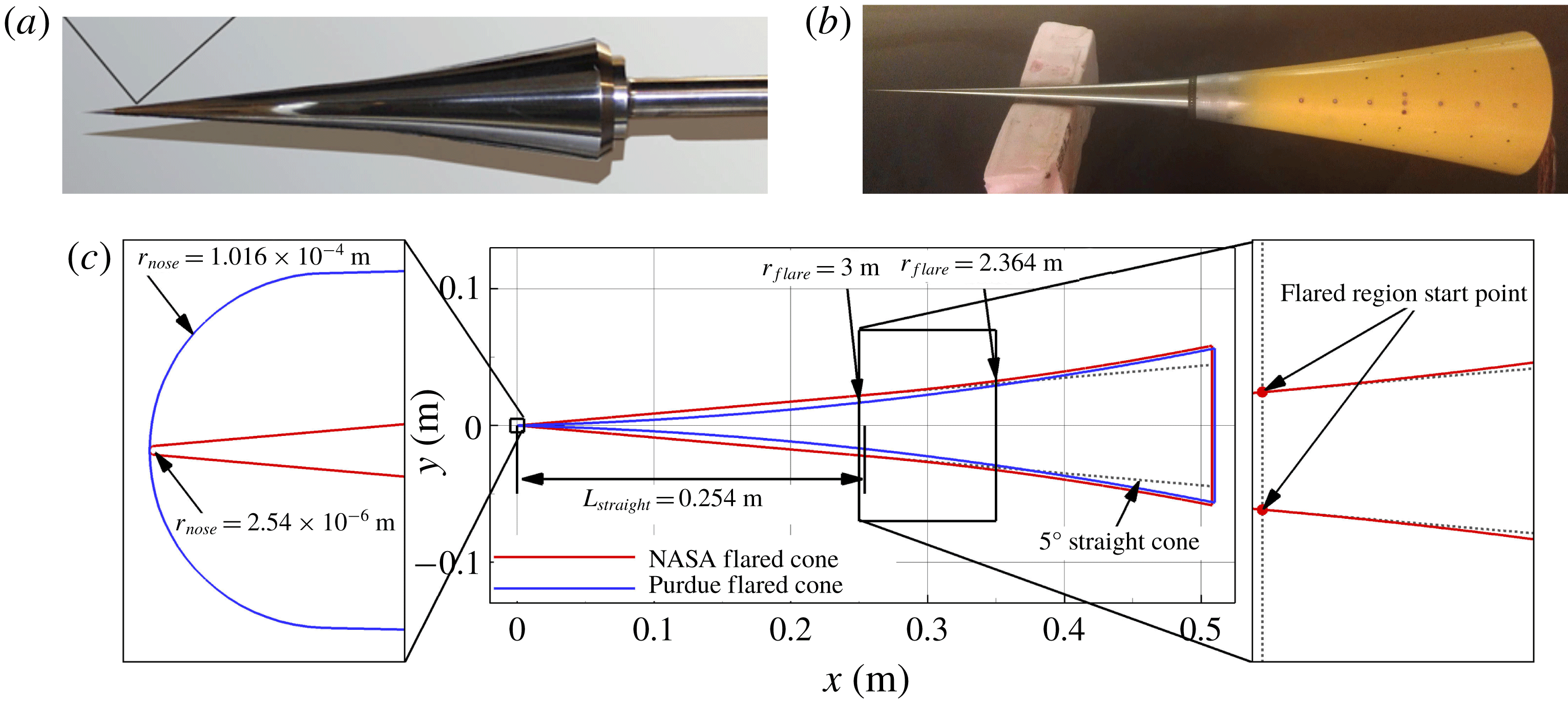
-half-angle sharp-nose straight cone section, which then changed into a circular arc flare portion for the remainder downstream extent of the cone. This cone geometry will be referred to as the ‘NASA flared cone’ (figure 3
a). They found that the transition process was dominated by second-mode waves. Blanchard, Selby & Wilkinson (Reference Blanchard, Selby and Wilkinson1996) carried out hypersonic stability experiments for the NASA flared cone with an adiabatic and a cooled wall in a quiet flow at the M6NTC and found that for the cooled-wall case the dominant second-mode frequency is higher and leads to larger integrated spatial growth rates (
 $N$
-factors) compared to the adiabatic-wall case. Doggett, Chokani & Wilkinson (Reference Doggett, Chokani and Wilkinson1997) investigated the stability behaviour for the NASA flared cone at angle of attack in the M6NTC. At the windward meridian of the model, they found that the boundary layer remained laminar over the entire length and that the frequency of the dominant second-mode instability increased relative to the case with zero angle of attack. They speculated that the dominant instability mechanism on the leeward meridian is not due to second-mode waves. Pruett & Chang (Reference Pruett and Chang1998) performed direct numerical simulations (DNS) for the conditions reported in Lachowicz et al. (Reference Lachowicz, Chokani and Wilkinson1996a
,Reference Lachowicz, Chokani and Wilkinson
b
). The results of the numerical simulations were consistent with the results of the experimental studies. Balakumar & Kegerise (Reference Balakumar and Kegerise2010) investigated the effect of the cone flare on receptivity and stability in a high-speed boundary layer at Mach 6. They found that the receptivity for sharp-nose geometries was orders of magnitude larger compared to the geometry with a blunt nose. The cone flare was found to have mainly two primary effects: The frequency of the most amplified second-mode disturbance shifted to a higher value compared to its straight cone counterpart, and the amplification rates of the first- and second-mode waves increased due to the cone flare. Laible & Fasel (Reference Laible and Fasel2011) carried out high-resolution DNS to study the effects of the cone flare on the nonlinear breakdown process at Mach 6 for the NASA flared cone and the M6NTC conditions. They observed streaks on the cone surface indicating local regions of high heat transfer. The M6NTC facility was moved to Texas A&M, and is now referred to as the Texas A&M Mach 6 Quiet Tunnel (M6QT), where Hofferth & Saric (Reference Hofferth and Saric2012) repeated some of the experiments for the NASA flared cone by Lachowicz et al. (Reference Lachowicz, Chokani and Wilkinson1996a
,Reference Lachowicz, Chokani and Wilkinson
b
) for quiet flow. They found that for quiet flow conditions transition occurred far downstream and very close to the base of the cone.
Picture of the NASA flared cone model (taken from Horvath et al. Reference Horvath, Berry, Hollis, Chang and Singer2002) (a), a picture of the Purdue flared cone model (taken from Chynoweth Reference Chynoweth2015) (b) and a comparison of the flared cone models between the NASA flared cone and the Purdue flared cone (c).

Wheaton et al. (Reference Wheaton, Juliano, Berridge, Chou, Gilbert, Casper, Steen and Schneider2009) designed a new flared cone geometry to experimentally investigate laminar–turbulent transition in the BAM6QT at Purdue University. This geometry differs from the NASA flared cone geometry in that the circular arc flare was applied along the entire length of the cone starting at the tip. This new geometry will be referred to as the ‘Purdue flared cone’ (figure 3
b). A comparison of the cone models in figure 3(c) shows that the Purdue flared cone is initially more slender and the curvature in the streamwise direction is larger compared to the NASA flared cone. The nominal nose radius of the NASA flared cone is
 $r_{nose}=2.54\times 10^{-6}~\text{m}$
and thus forty times smaller than the nominal nose radius of the Purdue flared cone with
 $r_{nose}=1.016\times 10^{-4}~\text{m}$
. Both cones, however, can be considered as ‘sharp’ according to the criterion used at NASA Langley (
 $Re_{r_{nose}}\leqslant 1000$
, Chynoweth Reference Chynoweth2015).
DNS of the laminar–turbulent breakdown for the Purdue flared cone and BAM6QT experimental conditions were reported by Fasel, Sivasubramanian & Laible (Reference Fasel, Sivasubramanian and Laible2015). They found that both the fundamental breakdown and the oblique breakdown scenario are viable paths to transition. In addition, the typical ‘hot’ streak pattern found by Laible (Reference Laible2011), Laible & Fasel (Reference Laible and Fasel2011) was confirmed as well. In experimental investigations Berridge et al. (Reference Berridge, Chou, Ward, Steen, Gilber, Juliano and Schneider2010) used the same cone geometry with a sharp nose as Wheaton et al. (Reference Wheaton, Juliano, Berridge, Chou, Gilbert, Casper, Steen and Schneider2009). In their experiments they were able to observe the development of ‘hot’ streaks on the cone surface, thus confirming the DNS results by Laible (Reference Laible2011) and Laible & Fasel (Reference Laible and Fasel2011). Experiments to investigate the influence of isolated roughness elements on the spacing of the streamwise streaks were carried out by Chou (Reference Chou2010), Ward et al. (Reference Ward, Wheaton, Chou, Gilbert, Steen and Schneider2010) and Chou et al. (Reference Chou, Ward, Letterman and Luersen2011). They found that ‘proper’ placing of the roughness elements can change the streamwise streak spacing and match the azimuthal spacing of the roughness dots. Li et al. (Reference Li, Choudhari, Chang and White2010a
,Reference Li, Choudhari, Chang, Wu and Greene
b
) performed numerical studies for the Purdue flared cone and the BAM6QT conditions that showed that both subharmonic and fundamental secondary instability can lead to large
 $N$
-factors. An extensive study by Li et al. (Reference Li, Choudhari, Chang and White2012) on the secondary instability for the Purdue flared cone at Mach 6 using nonlinear parabolized stability equations (PSE) indicated that the fundamental resonance led to larger amplification rates and
 $N$
-factors of the secondary disturbance wave compared to the subharmonic resonance scenario. The authors suggested that it will be important to determine the role of fundamental modes in the transition process. Terwilliger (Reference Terwilliger2011) investigated the fundamental and oblique breakdown scenarios for the Purdue flared cone geometry and the BAM6QT conditions using DNS. He also observed the development of ‘hot’ streaks and found good qualitative agreement between DNS and experimental results. Berridge et al. (Reference Berridge, Ward, Luersen, Chou, Abney and Schneider2012) and Luersen (Reference Luersen2012) investigated techniques for applying roughness elements onto the flared cone geometry in order to improve repeatability of the experiments. The epoxy dot technique turned out to be not suitable to generate adequately sized roughness elements. Ward et al. (Reference Ward, Wheaton, Chou, Berridge, Letterman, Luersen and Schneider2012) observed transition under quiet conditions on a flared cone at Mach 6 and captured the typical pattern of ‘hot’ streaks appearing, disappearing and reappearing. Chynoweth et al. (Reference Chynoweth, Ward, Greenwood, McKiernan, Fisher and Schneider2014a
,Reference Chynoweth, Ward, Henderson, Moraru, Greenwood, Abney and Schneider
b
), Chynoweth (Reference Chynoweth2015) and McKiernan, Chynoweth & Schneider (Reference McKiernan, Chynoweth and Schneider2015) continued the investigations of the influence of roughness elements on the streak development. They found that the roughness elements interact with the second-mode waves without tripping the boundary layer, and that the streak spacing could be successfully modified with the roughness elements.
At this point it is not clear what physical mechanisms cause the streak development, why the streaks appear, disappear and reappear in the breakdown region. Most important is an answer to the question if the streaks observed in the experiments are caused by the nonlinear mechanisms investigated by Laible (Reference Laible2011) who found that streak patterns can be generated by either a so-called ‘oblique breakdown’ (Fasel, Thumm & Bestek Reference Fasel, Thumm and Bestek1993) as well as a so-called ‘fundamental breakdown’.
The objective of this research is to provide clear evidence that the ‘hot’ streaks in the experiments are caused by the same nonlinear mechanisms as in the DNS. Towards this end, detailed investigations using high-fidelity DNS of the underlying nonlinear mechanisms were carried out in order to understand what exactly causes the ‘hot’ streaks. An extensive flow field analysis was performed in support of the ongoing experiments. The cone geometry and the flow conditions for the present investigation are chosen to match as closely as possible those of the experimental investigations currently carried out at the Purdue University BAM6QT facility.
2 Simulation strategy
The simulation strategy for carrying out the stability and transition investigations can be broken down into three main steps.
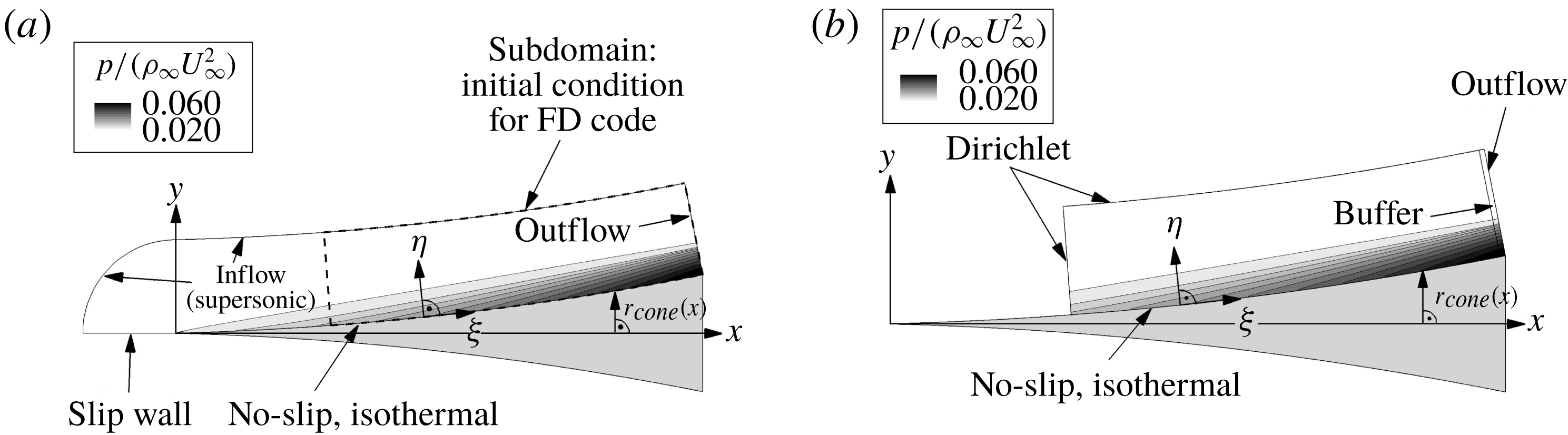
First, an initial, undisturbed base flow is obtained from a precursor calculation using a finite volume (FV) code developed in our computational fluid dynamics (CFD) laboratory at the University of Arizona (Gross & Fasel Reference Gross and Fasel2002, Reference Gross and Fasel2008, Reference Gross and Fasel2010a ,Reference Gross and Fasel b ). In the precursor calculation the entire cone geometry is considered, including the nose of the cone (see figure 4 a).
In the second step, a higher-order finite difference (FD) calculation (Laible Reference Laible2011; Laible & Fasel Reference Laible and Fasel2011) is performed. For the FD calculation, the computational domain starts downstream of the tip of the cone as shown in figure 4(b). For this the solution obtained with the FV code is interpolated (second-order interpolation) onto a finer grid and then used in the FD calculation as initial guess and for the inflow and free-stream boundary condition. This FD calculation is performed in order to obtain a ‘clean’ base-flow state for the final third step.
Computational domain used for the base-flow computation with the finite volume (FV) code (a) and the finite difference (FD) code (b).

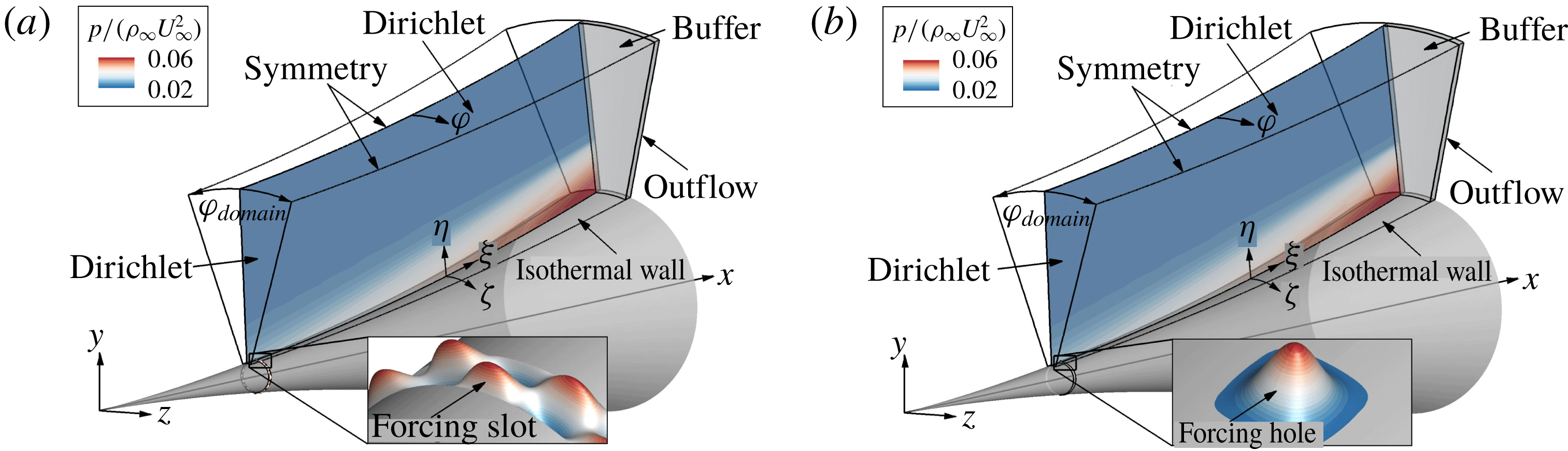
In the third step the disturbance (transition) simulations are carried out using the same FD code as in step 2 (Laible Reference Laible2011; Laible & Fasel Reference Laible and Fasel2011). The re-converged base flow from the second step is used as an initial condition. Schematics of the computational domain used for disturbance simulations are provided in figure 5. The disturbances are introduced either through a blowing/suction slot or hole at the wall downstream of the inflow boundary, or time-dependent boundary conditions at the inflow (Fasel Reference Fasel1976), or combinations thereof. When using a forcing slot or hole, the disturbances are introduced via perturbations of the wall normal velocity (
 $v^{\prime }$
), whereas for the time-dependent inflow boundary conditions the wall-normal amplitude and phase distributions of all primitive flow variables are used, which are either obtained through a precursor simulation or by solving the compressible linear stability theory (LST) equations.
Computational set-up for disturbance simulations using the finite difference code (Laible Reference Laible2011) for a continuous forcing simulation (a), and a short duration pulse forcing (b).

For the results presented in this paper the perturbations were introduced downstream of the inflow boundary using two different temporal and spatial forcing functions. In a first option, wall-normal velocity disturbances are introduced continuously (2.1) through a forcing ‘slot’ at the wall (figure 5 a) in order to introduce a specified single frequency or a specified set of frequencies into the computational domain,
 $$\begin{eqnarray}v^{\prime }(t)/U_{\infty }=\mathop{\sum }_{i=1}^{n}A_{forcing,i}\cos (\unicode[STIX]{x1D714}_{forcing,i}t+\unicode[STIX]{x1D719}_{i}),\end{eqnarray}$$
where
 $n$
is the number of frequencies to be forced,
 $\unicode[STIX]{x1D714}_{forcing,i}$
is the angular forcing frequency (
 $\unicode[STIX]{x1D714}_{forcing,i}=2\unicode[STIX]{x03C0}f_{forcing,i}$
),
 $\unicode[STIX]{x1D719}_{i}$
is a user-specified phase shift and
 $A_{forcing,i}$
is the forcing amplitude of the
 $i$
th frequency component. Another option to generate the wall-normal velocity disturbances is to introduce a broad range of frequencies and azimuthal wavenumbers by applying a short duration pulse (2.2) through a ‘hole’ in the wall (figure 5
b).
 $$\begin{eqnarray}v^{\prime }(t)/U_{\infty }=\left\{\begin{array}{@{}ll@{}}A_{pulse}\cos (\unicode[STIX]{x1D714}_{pulse}t+\unicode[STIX]{x1D719}) & t\leqslant T_{pulse}\\ 0 & t>T_{pulse},\end{array}\right.\end{eqnarray}$$
where
 $T_{pulse}$
is the forcing duration,
 $\unicode[STIX]{x1D714}_{pulse}=2\unicode[STIX]{x03C0}f_{pulse}=2\unicode[STIX]{x03C0}/T_{pulse}$
is the angular frequency around which the pulse is centred and
 $A_{pulse}$
is the initial forcing amplitude of the short duration pulse.
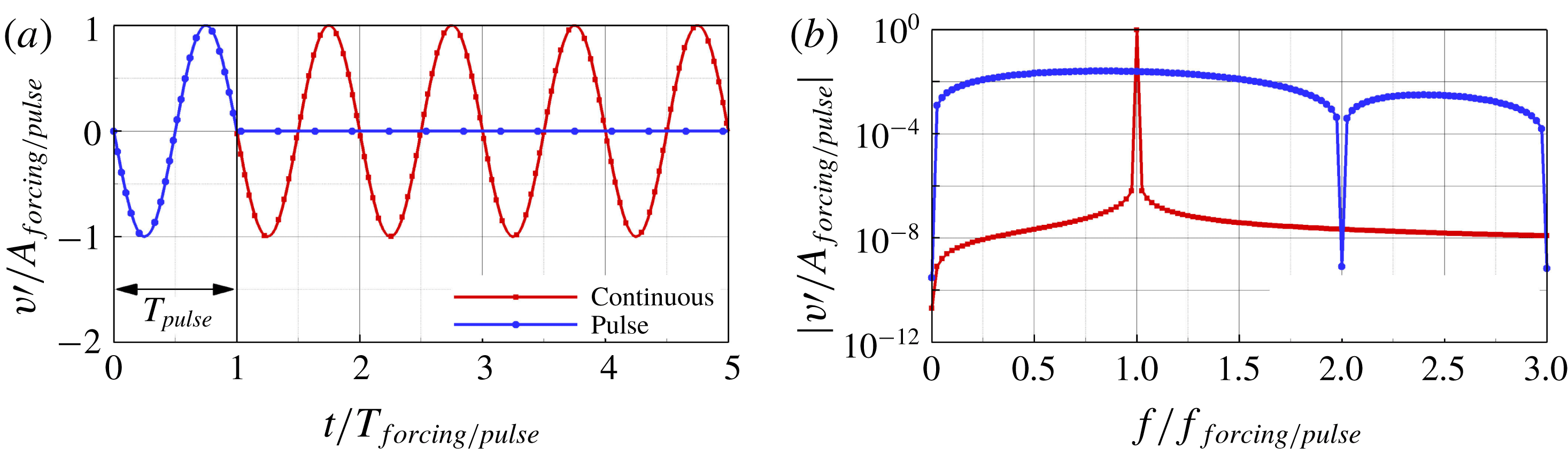
The normalized wall-normal velocity perturbation versus time at the forcing location for the continuous and short duration pulse forcing are shown in figure 6(a). In this example only one frequency is introduced with the continuous forcing approach. The corresponding amplitude spectra of the two different forcing functions are provided in figure 6(b). The spectra highlight the key differences between the two approaches. While the continuous forcing essentially introduces only a single frequency, the pulse forcing results in a broad spectrum. With the continuous forcing the disturbance frequencies that are introduced into the computational domain can be controlled accurately, thus allowing so-called ‘controlled’ breakdown simulations.
Wall-normal velocity disturbance evolution (a), and corresponding amplitude spectra (b) for the continuous and short duration pulse forcing approach.

3 Numerical methods
The details of the DNS code used here, along with its continuing development, have been described in Laible, Mayer & Fasel (Reference Laible, Mayer and Fasel2008, Reference Laible, Mayer and Fasel2009), Laible (Reference Laible2011), Laible & Fasel (Reference Laible and Fasel2011). Therefore, only a short overview will be given. The numerical method is based on the three-dimensional (3-D) Navier–Stokes equations, the continuity equation and the energy equation for a compressible fluid in generalized conical coordinates. The so-called spatial model is applied, where all three spatial dimensions and time are discretized without any modelling assumptions. High-order accurate non-compact central finite differences are used for discretization of the wall-normal (fourth-order) and the streamwise direction (sixth-order). In the azimuthal direction, a pseudo-spectral discretization using fast Fourier transforms is employed. The inviscid fluxes are separated into an upwind flux and a downwind flux using van Leer’s splitting (van Leer Reference van Leer1982). Then, grid centred upwind biased differences (Zhong Reference Zhong1998) with ninth-order accuracy are applied to evaluate the derivatives for these fluxes. Special attention is given to the wall-next boundary stencils. Since high-order accurate boundary closures are typically unstable, the order of the stencil is successively reduced from ninth order to third order at the wall. For further details, the reader is referred to the references given above.
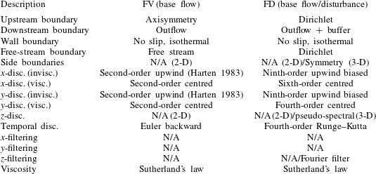
The boundary conditions together with the spatial and temporal discretization used in the three steps of the simulation procedure for the results discussed in this paper are provided in table 1. The wall is assumed to be isothermal for the base flow and will remain so even in the presence of the disturbances. Consequently, the temperature disturbances at the wall vanish. The isothermal-wall assumption with respect to the disturbances is justified because the wall temperature of the model remains nearly constant in the experiments due to the very short run times of the BAM6QT (see Ward Reference Ward2010; Chynoweth Reference Chynoweth2015).
Boundary conditions, spatial and temporal discretization employed for the simulations (disc.
 $=$
discretization, invisc.
 $=$
inviscid terms, visc.
 $=$
viscous terms).

4 Flow conditions and cone geometry
The transition investigations presented here are based on the Purdue flared cone geometry with a 4.5 inch base diameter that is used for the ongoing experiments in the BAM6QT (Chynoweth et al.
Reference Chynoweth, Ward, Greenwood, McKiernan, Fisher and Schneider2014a
,Reference Chynoweth, Ward, Henderson, Moraru, Greenwood, Abney and Schneider
b
; Chynoweth Reference Chynoweth2015; McKiernan et al.
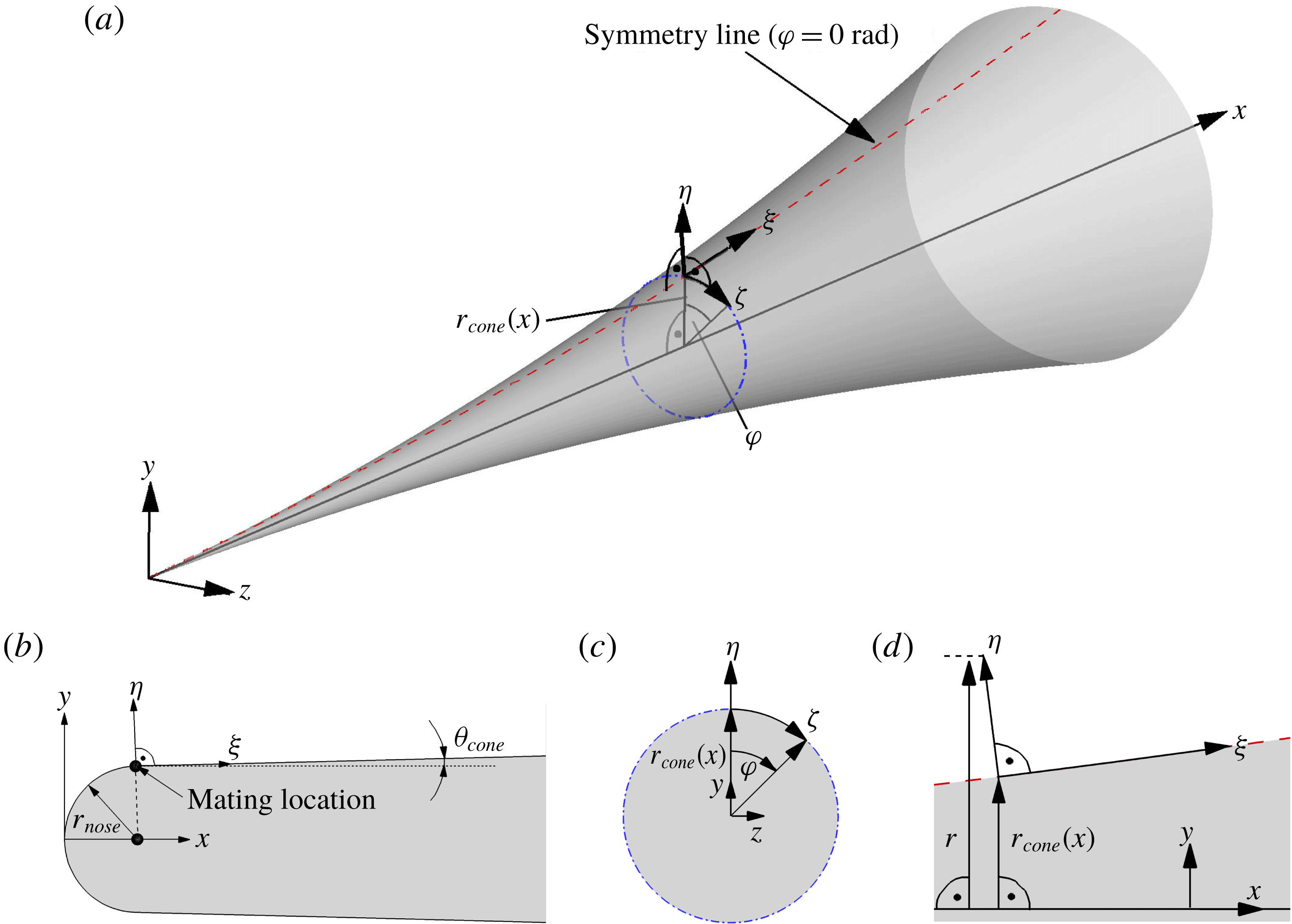
Reference McKiernan, Chynoweth and Schneider2015). Here, the flared cone is considered at a zero angle of attack. A schematic of the flared cone and the reference coordinate systems is provided in figure 7. The origin of the Cartesian coordinate system (
 $x,y,z$
) is at the nose of the cone with the
 $x$
axis along the axis of the cone. A body-fitted coordinate system (
 $\unicode[STIX]{x1D709},\unicode[STIX]{x1D702},\unicode[STIX]{x1D701}$
) is defined by the coordinate
 $\unicode[STIX]{x1D709}$
along the surface of the cone, the coordinate
 $\unicode[STIX]{x1D702}$
in the radial direction normal to the surface of the cone and the azimuthal coordinate
 $\unicode[STIX]{x1D701}$
, which is defined as
 $$\begin{eqnarray}\unicode[STIX]{x1D701}=\unicode[STIX]{x1D711}r_{cone}(x),\end{eqnarray}$$
where
 $\unicode[STIX]{x1D711}$
is the azimuthal angle and
 $r_{cone}(x)$
is the local radius of the cone measured from the body axis (
 $x$
) to the surface of the cone. The azimuthal coordinate
 $\unicode[STIX]{x1D701}$
is often referred to as the unrolled cone coordinate. The initial half-angle of the cone is indicated in the schematic of figure 7(b). It is defined as the angle between the horizontal axis and the tangent to the circular arc flare region of the cone at the so-called mating location between the nose, which is modelled by a section of a circle, and the circular arc flare region. The close up of a cross-section of the flared cone in a plane perpendicular to the
 $x$
-axis (figure 7
c) provides details regarding the geometric relationship of the unrolled cone coordinate (
 $\unicode[STIX]{x1D701}$
), the azimuthal angle (
 $\unicode[STIX]{x1D711}$
) and the local cone radius (
 $r_{cone}(x)$
). A side view of a small section of the cone in figure 7(d) indicates the relationship of the local radial coordinate,
 $r$
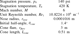
, measured perpendicular to the cone axis to a point above the cone surface in the flow field. This radial coordinate is used to unroll the azimuthal direction for data extracted parallel to the cone surface. The flow conditions and cone geometry parameters are provided in table 2. The fluid is a perfect gas (air) with a ratio of specific heats of
 $\unicode[STIX]{x1D6FE}=1.4$
and a Prandtl number of
 $Pr=0.71$
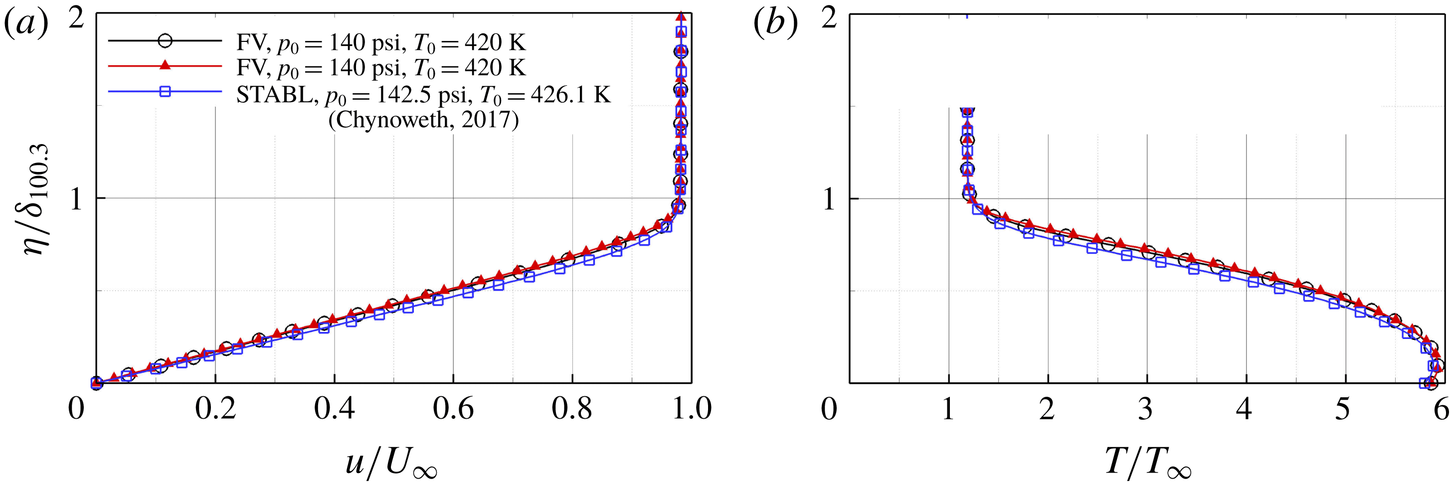
. The nose of the cone is resolved with 20 points, which is assumed to be sufficient based on the results of Terwilliger (Reference Terwilliger2011) for a similar cone geometry. A comparison between the normalized base-flow profiles computed with the FV code, the FD code and the STABL software suite (Stability and Transition Analysis for hypersonic Boundary Layers, see Johnson & Candler Reference Johnson and Candler2005) provided by (B. C. Chynoweth, private communication 2017) is shown in figure 8. The wall-normal coordinate was normalized with the local boundary-layer thickness determined as the location where 100.3 % of the total enthalpy is reached (
 $\unicode[STIX]{x1D6FF}_{100.3}$
, see for example Meersman, Hader & Fasel Reference Meersman, Hader and Fasel2018). The profiles for the streamwise velocity component (figure 8
a) and temperature (figure 8
b) obtained with the different codes are in reasonable agreement suggesting that the basic state obtained from the FD calculation was sufficiently ‘clean’ so as to be used for the initial and boundary conditions for the disturbance simulations.
Schematic of the flared cone geometry showing the different coordinate systems (a), and close ups of the nose region (b), a cut through the cone along the cone axis (c) and a cone cross-section (d) to illustrate the geometric relationships between the different coordinate systems.

Comparison of the normalized
 $u$
-velocity base-flow profiles (a), and the normalized temperature base-flow profiles (b) extracted at
 $x=0.2570~\text{m}$
, between the FD code, the FV code and the STABL solution (B. C. Chynoweth, personal communication 2017).

5 Mode terminology
For the analysis of the breakdown simulations a mode terminology
 $(n,m)$
is employed. Here
 $n$
is the multiple of the primary wave frequency,
 $f_{primary}$
. For the presented ‘controlled’ disturbance simulations, the frequency chosen for
 $f_{primary}$
was that which led to the largest
 $N$
-factors based on the results of the low amplitude (linear) pulse calculations as discussed below in § 6.1. The integer
 $m$
is the multiple of the spanwise ‘domain wavenumber’, which denotes the lowest azimuthal wavenumber that can be represented on the grid employed for the disturbance simulations,
 $$\begin{eqnarray}k_{c,domain}=\frac{2\unicode[STIX]{x03C0}}{\unicode[STIX]{x1D711}_{domain}}.\end{eqnarray}$$
Thus
 $k_{c,domain}$
depends on the azimuthal extent,
 $\unicode[STIX]{x1D711}_{domain}$
, of the computational domain (figure 5).
Flow conditions and details of the cone geometry for BAM6QT experiments (Chynoweth et al. Reference Chynoweth, Ward, Greenwood, McKiernan, Fisher and Schneider2014a ,Reference Chynoweth, Ward, Henderson, Moraru, Greenwood, Abney and Schneider b ; Chynoweth Reference Chynoweth2015; McKiernan et al. Reference McKiernan, Chynoweth and Schneider2015).

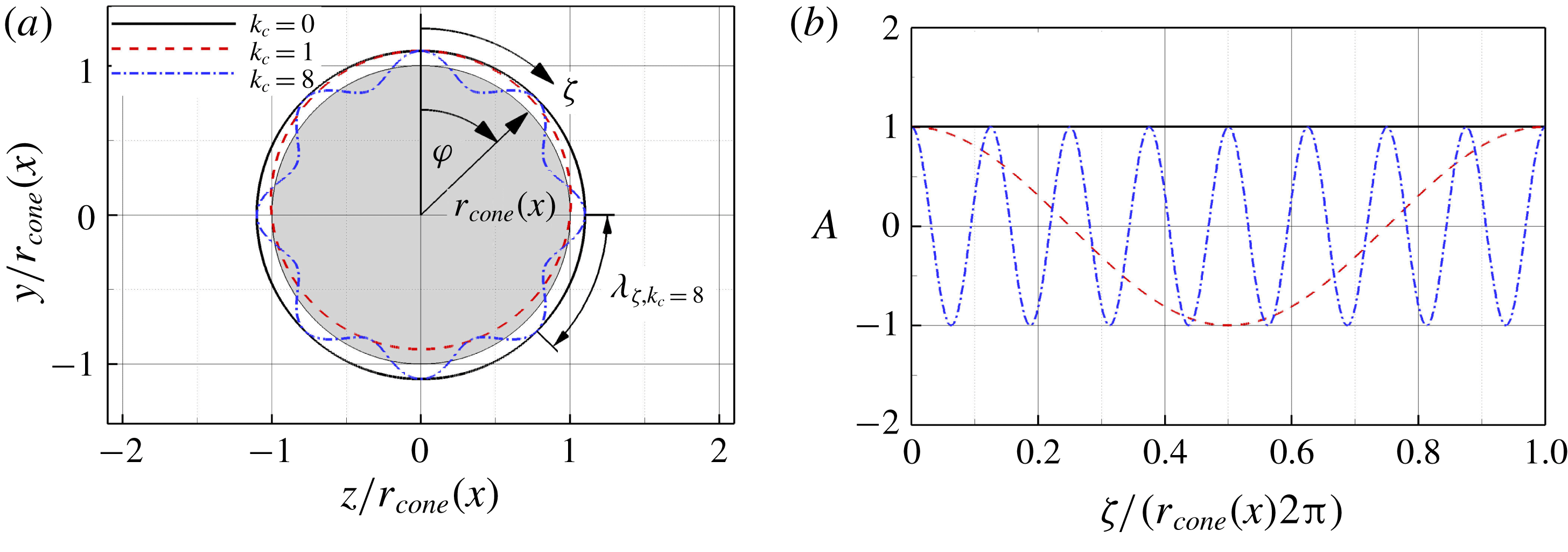
The concept of the azimuthal wavenumber is illustrated in figure 9. It represents the number of wavelengths of an azimuthal wave around the circumference of the cone (figure 9
a). For axisymmetric geometries, such as the flared cone considered here, the azimuthal wavenumber can only have an integer value. Plotting the azimuthal waves in the unrolled cone coordinate
 $\unicode[STIX]{x1D701}$
(4.1) normalized with the local cone circumference (figure 9
b) shows that a wave with the azimuthal wavenumber
 $k_{c}=0$
is two-dimensional (axisymmetric) without any modulation in the azimuthal direction (constant amplitude), whereas a wave with an azimuthal wavenumber of
 $k_{c}=q$
has exactly
 $q$
wavelengths around the circumference of the cone.
For a constant azimuthal wavenumber, the azimuthal wavelength changes with the local radius due to body divergence according to
 $$\begin{eqnarray}\unicode[STIX]{x1D706}_{\unicode[STIX]{x1D701}}=\frac{2\unicode[STIX]{x03C0}r_{cone}(x)}{k_{c}}.\end{eqnarray}$$
The cone radius,
 $r_{cone}(x)$
, increases in the downstream direction. Consequently, the wave angle (
 $\unicode[STIX]{x1D713}=\arctan (\unicode[STIX]{x1D706}_{x}/\unicode[STIX]{x1D706}_{\unicode[STIX]{x1D701}})$
) for a wave of constant
 $k_{c}$
is continuously decreasing in the downstream direction.
Illustration of a geometry cross-section and the azimuthal wavenumber,
 $k_{c}$
, (a), and the azimuthal wave in the unrolled coordinate (
 $\unicode[STIX]{x1D701}$
) for different values of
 $k_{c}$
(b).

In summary, the mode terminology (
 $n,m$
) employed here is thus a shorthand notation for (
 $n\cdot f_{primary},m\cdot k_{c,domain}$
). Note also that, due to the symmetry conditions employed at the azimuthal domain boundaries, only half of the computational domain (
 $\unicode[STIX]{x1D711}_{domain}$
) needs to be used in the simulations (
 $\unicode[STIX]{x1D711}_{sim.}=\unicode[STIX]{x1D711}_{domain}/2$
, figure 5).
6 ‘Controlled’ breakdown simulations
As stated in the introduction, Schneider (Reference Schneider2015) pointed out the need for numerical studies in combination with quiet tunnel experiments for understanding hypersonic transition and for developing physics based transition prediction methods. Towards this end, high-fidelity DNS were carried out for the BAM6QT conditions to understand the nonlinear mechanisms leading to breakdown and ultimately to turbulence. As a model of the natural transition scenario observed in the experiments at the BAM6QT, the DNS were performed using a ‘controlled’ disturbance input. In order to determine the ‘appropriate’ (i.e. relevant for experiments) disturbance input for such so-called ‘controlled transition simulations’, the primary and secondary instability regimes were investigated prior to carrying out the high-resolved DNS for the entire transition process including the breakdown to turbulence. The dominant primary instability mechanism for the Mach number considered here (
 $M=6$
) is due to second-mode waves (Mack Reference Mack1969). Thus, second mode waves will dictate the primary wave frequency prior to the onset of the secondary instability and therefore the disturbance input parameters for the controlled transition simulations.
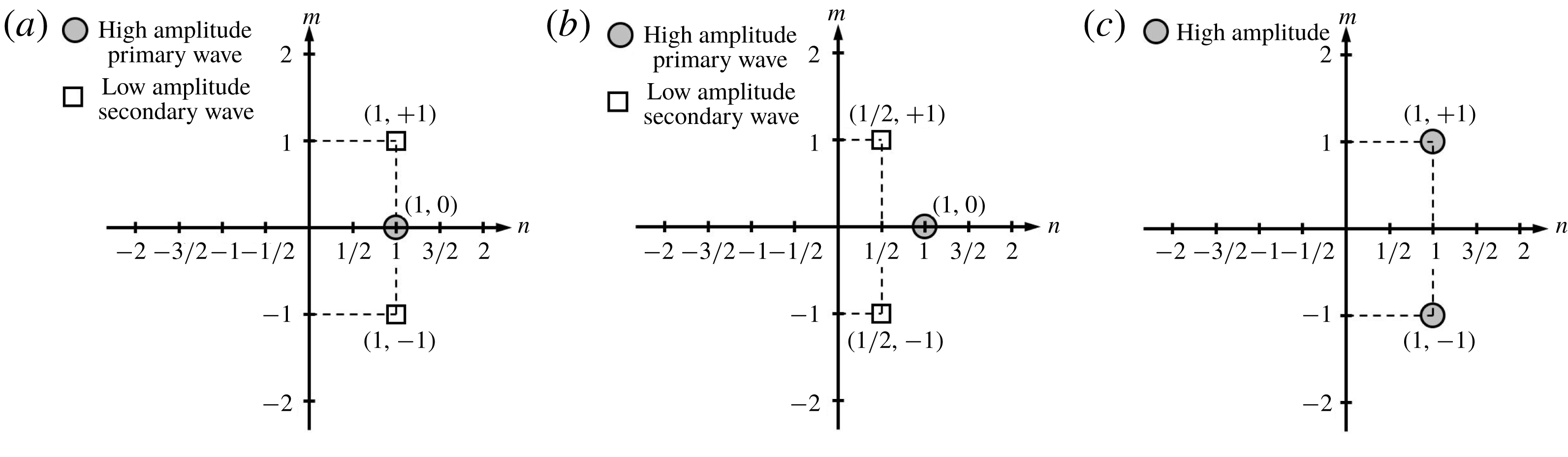
To initiate laminar–turbulent transition in the DNS the disturbances have to be introduced into the computational domain. Towards this end, two different approaches are employed in the present study as discussed in § 2. Initiating the breakdown by disturbances consisting of a specific set of frequencies and azimuthal wavenumbers using the continuous forcing approach is referred to as ‘controlled’ breakdown. Three different ‘controlled’ breakdown scenarios that have been found in past research (Craik Reference Craik1971; Herbert Reference Herbert1988; Kachanov Reference Kachanov1994) to be relevant for the nonlinear transition stages for low-speed (incompressible) boundary layers are schematically depicted in the frequency–wavenumber diagrams of figure 10.
The so-called fundamental resonance (figure 10
a) is initiated with a large amplitude, two-dimensional primary wave, (
 $1,0$
), and a pair of small amplitude oblique secondary disturbance waves at the same (fundamental) frequency as the primary wave, (
 $1,\pm 1$
). This resonance was originally found to be relevant for incompressible boundary layers when the free-stream turbulence level is slightly elevated and in that context is also referred to as Klebanoff (
 $K$
-) type breakdown (Klebanoff, Tidstrom & Sargent Reference Klebanoff, Tidstrom and Sargent1962; Bake, Meyer & Rist Reference Bake, Meyer and Rist2002).
In contrast, for the so-called subharmonic resonance (figure 10
b) a two-dimensional primary wave, (
 $1,0$
), is forced at a large amplitude along with a pair of small amplitude secondary oblique waves at half (subharmonic) of the frequency of the primary wave, (
 $1/2,\pm 1$
). This resonance was originally found to be relevant for incompressible boundary layers when the free-stream turbulence level is low (lower than for
 $K$
-type) and in that context is referred to as Herbert (
 $H$
-) type breakdown (Kachanov & Levchenko Reference Kachanov and Levchenko1984).
For the oblique breakdown only a pair of large amplitude three-dimensional disturbance waves (
 $1,\pm 1$
) is required to initiate nonlinear resonances. This breakdown was originally discovered for a flat plate boundary layer at
 $M=1.6$
(Fasel et al.
Reference Fasel, Thumm and Bestek1993) and found later to also be relevant for cone boundary layers at
 $M=8$
(Pruett & Chang Reference Pruett and Chang1995).
In the present paper the focus is on the fundamental breakdown. The primary and secondary wave frequencies were chosen based on the (primary) linear stability investigations as discussed in § 6.1. For selecting the azimuthal wavenumber for the secondary oblique waves, a parameter study was carried out as discussed in § 6.2.
Frequency–wavenumber schematic for the fundamental breakdown (a), the subharmonic breakdown (b) and the oblique breakdown (c).

6.1 Primary instability
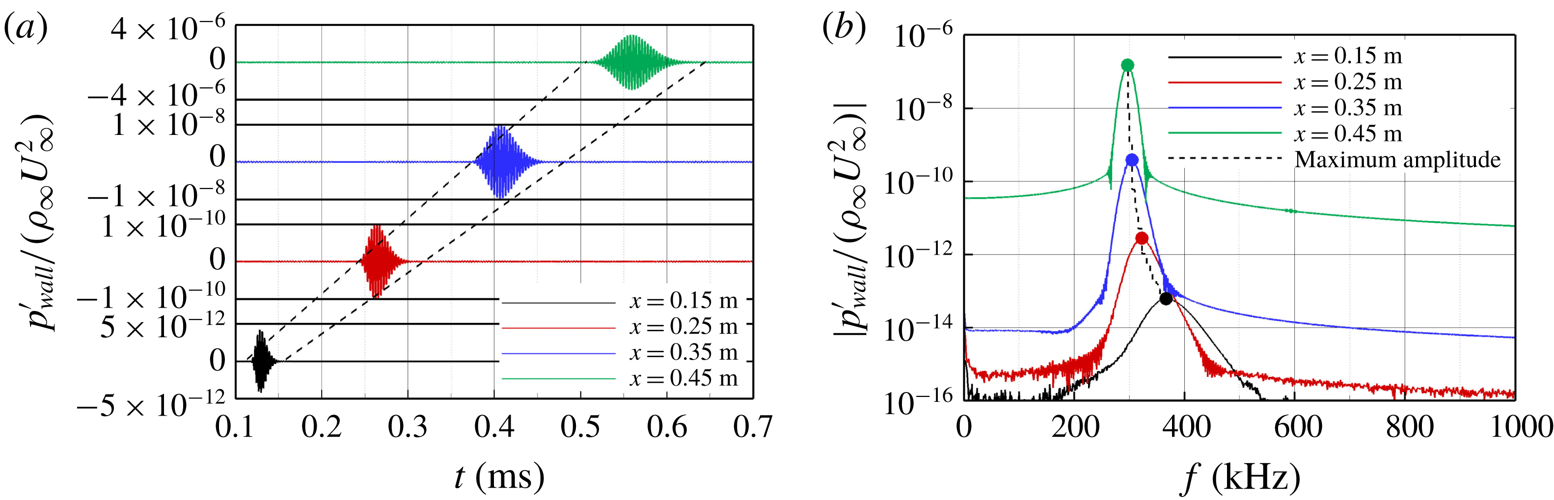
For selecting a proper frequency to be used for the ‘controlled’ fundamental breakdown simulations, first the linear stability regime was investigated. Towards this end, a low amplitude, axisymmetric pulse calculation was carried out for typical BAM6QT experimental conditions (Chynoweth et al. Reference Chynoweth, Ward, Greenwood, McKiernan, Fisher and Schneider2014a ,Reference Chynoweth, Ward, Henderson, Moraru, Greenwood, Abney and Schneider b ; Chynoweth Reference Chynoweth2015; McKiernan et al. Reference McKiernan, Chynoweth and Schneider2015) as provided in table 2. The pulse calculations are used to identify the most unstable frequency band. The short duration pulse is introduced into the domain through a blowing and suction hole in the wall using wall-normal velocity disturbances (figure 5 b). Due to the short duration of the pulse, a wide range of frequencies is introduced into the boundary layer (see figure 6 b) which then begin to form a wave packet. The wave packet is tracked in the downstream direction as it propagates through the computational domain.
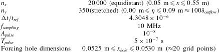
Details of the simulation parameters for the axisymmetric pulse calculation are provided in table 3. The resolution in streamwise direction is high enough to resolve the high frequency wave components with a sufficient number of points. In addition, the sampling frequency is chosen such that frequencies up to 1 MHz are resolved with at least 10 sampling time steps in order to minimize aliasing errors and spectral leakage when computing the spectra. The extent of the computational domain for the axisymmetric pulse calculations in the streamwise direction was chosen so that the entire linear stability regime could be analysed using the high-order finite difference code. The nose of the cone was excluded for the stability calculations as discussed in § 2. The forcing hole was located approximately 100 grid points downstream of the inflow boundary to avoid possible reflections at the inflow boundary of upstream traveling waves. The wall pressure disturbance signals over time (figure 11
a) and their corresponding frequency spectra (figure 11
b) at different downstream locations show that the low amplitude wave packet spreads and significantly grows in amplitude when propagating in the downstream direction. One of the main reasons for using flared cones in hypersonic boundary-layer transition research is to keep the boundary-layer thickness at an approximately constant value such that the most amplified frequencies are nearly constant in downstream direction (Wheaton et al.
Reference Wheaton, Juliano, Berridge, Chou, Gilbert, Casper, Steen and Schneider2009). This ultimately leads to higher
 $N$
-factors for a shorter downstream distance compared to a ‘straight’ (non-flared) cone. The spectra shown in figure 11(b) confirm that a relatively narrow frequency band emerges around 300–350 kHz and is amplified along the entire length of the cone. The
 $N$
-factors are computed according to van Ingen (Reference van Ingen2008) as
 $N=\ln (A(x)/A(x_{0}))$
, where
 $A$
is a place holder for the amplitude and
 $x_{0}$
is defined as the reference position where the disturbance of a given frequency and amplitude
 $A(x_{0})$
becomes first unstable (van Ingen Reference van Ingen2008).
Time signals of the wall pressure disturbance (a), and corresponding amplitude spectra in frequency space (b) at different downstream locations.

Low amplitude pulse calculation set-up.

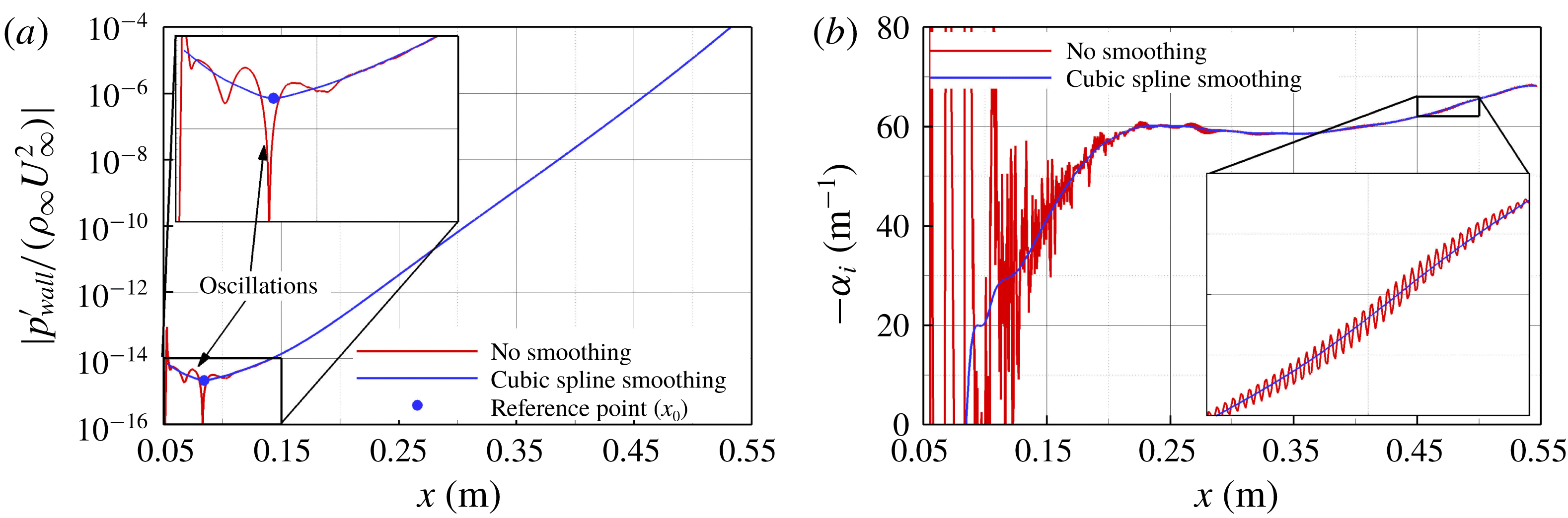
For the pulse calculations the reference position of a disturbance wave
 $x_{0}$
is difficult to determine unambiguously because of small oscillations in the downstream amplitude development (see figure 12
a). Simply using the location where amplification is first observed as the reference location
 $x_{0}$
would not correctly reproduce the criterion according to van Ingen (Reference van Ingen2008) because the disturbance wave is still decaying and the amplification at first only occurs for a limited downstream distance due to these oscillations. To determine an improved reference position, a cubic spline smoothing (Weinert Reference Weinert2009) was applied to the amplitude development in the downstream direction (figure 12
a), which eliminates these oscillations. The reference position and the
 $N$
-factors are then extracted from the smoothed amplitude curve. The spatial growth rate (
 $\unicode[STIX]{x1D6FC}_{i}$
) is calculated as the second-order numerical derivative of the natural logarithm of the pressure disturbance amplitude at the wall (
 $p_{wall}^{\prime }$
) for the various disturbance modes
 $(n,m)$
(see § 5) with respect to the body coordinate
 $\unicode[STIX]{x1D709}$
(figure 7
a)
 $$\begin{eqnarray}-\unicode[STIX]{x1D6FC}_{i_{i,(n,m)}}=\mathop{\sum }_{l=-1}^{1}c_{l}\ln (|p_{i+l,(n,m)}^{\prime }|_{wall}),\quad 2\leqslant i\leqslant n_{x},\end{eqnarray}$$
where
 $i$
is the grid index in the streamwise direction,
 $n_{x}$
is the number of grid points in the streamwise direction,
 $(n,m)$
denotes the disturbance mode frequency and azimuthal wavenumber and the stencil coefficients,
 $c_{l}$
, are determined at each grid point by solving a linear system of the form
 $$\begin{eqnarray}\left[\begin{array}{@{}ccc@{}}1 & 1 & 1\\ \unicode[STIX]{x1D709}_{i-1}-\unicode[STIX]{x1D709}_{i} & 0 & \unicode[STIX]{x1D709}_{i+1}-\unicode[STIX]{x1D709}_{i}\\ \displaystyle \frac{(\unicode[STIX]{x1D709}_{i-1}-\unicode[STIX]{x1D709}_{i})^{2}}{2} & 0 & \displaystyle \frac{(\unicode[STIX]{x1D709}_{i+1}-\unicode[STIX]{x1D709}_{i})^{2}}{2}\end{array}\right]\left(\begin{array}{@{}c@{}}c_{-1}\\ c_{0}\\ c_{1}\end{array}\right)=\left(\begin{array}{@{}c@{}}0\\ 1\\ 0\end{array}\right)\!.\end{eqnarray}$$
The spatial growth rates at the inflow and outflow boundaries were calculated using a first-order accurate difference scheme as
 $$\begin{eqnarray}\displaystyle & \displaystyle -\unicode[STIX]{x1D6FC}_{i_{1,(n,m)}}=\frac{|p_{2,(n,m)}^{\prime }|_{wall}-|p_{1,(n,m)}^{\prime }|_{wall}}{\unicode[STIX]{x1D709}_{2}-\unicode[STIX]{x1D709}_{1}} & \displaystyle\end{eqnarray}$$
 $$\begin{eqnarray}\displaystyle & \displaystyle -\unicode[STIX]{x1D6FC}_{i_{n_{x},(n,m)}}=\frac{|p_{n_{x},(n,m)}^{\prime }|_{wall}-|p_{n_{x}-1,(n,m)}^{\prime }|_{wall}}{\unicode[STIX]{x1D709}_{n_{x}}-\unicode[STIX]{x1D709}_{n_{x}-1}}. & \displaystyle\end{eqnarray}$$
A comparison between the spatial growth rate development calculated with the un-smoothed and smoothed amplitude curves is shown in figure 12(b). The cubic spline smoothing substantially reduces the ‘noise’ in the spatial growth rates, which is caused by the calculation of the numerical derivative, while accurately retaining the main trends. Consequently, the
 $N$
-factors and the spatial growth rates were computed after applying a cubic spline smoothing to the amplitude development.
Comparison of the amplitude (a), and the spatial growth rate (b) development in the downstream direction of the un-smoothed and smoothed (cubic spline smoothing) data for the
 $f=300~\text{kHz}$
disturbance wave.

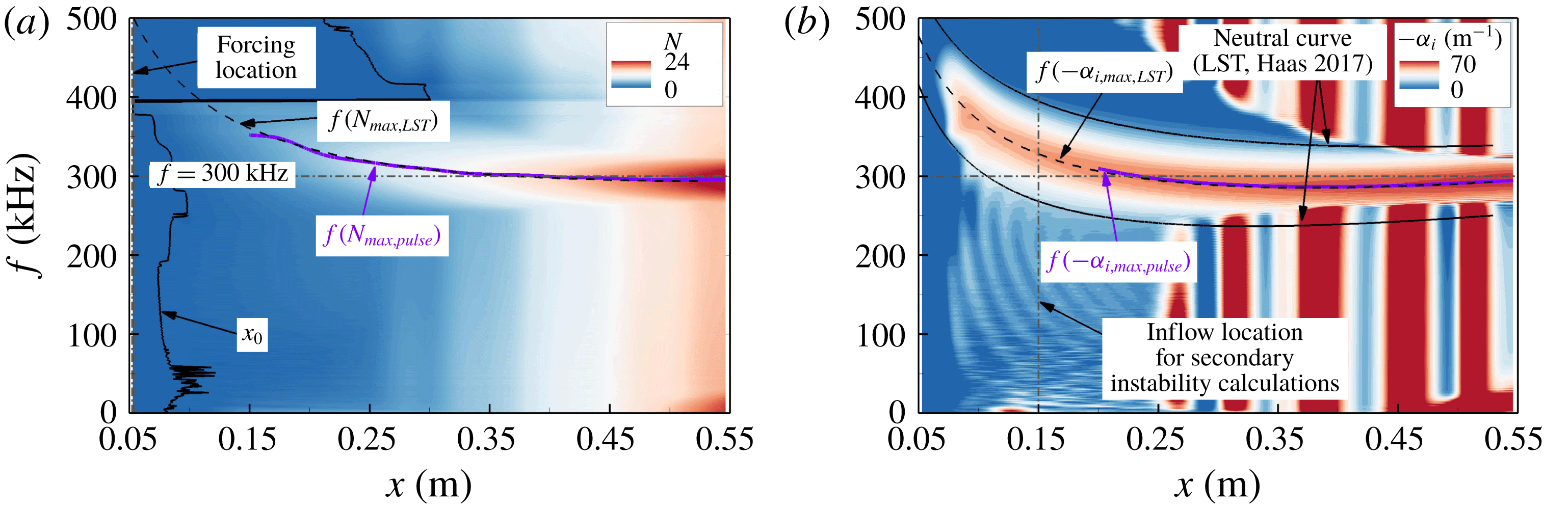
The
 $N$
-factor spectrum is provided in figure 13(a). For reference, the frequency for which the maximum
 $N$
-factor is obtained using LST is marked with a black dashed line (
 $f(N_{max,LST})$
) and the corresponding frequency resulting in the maximum
 $N$
-factor using the low amplitude pulse calculations is highlighted with a solid purple line (
 $f(N_{max,pulse})$
). The frequency leading to the maximum
 $N$
-factor drops from approximately 350 kHz at
 $x=0.15~\text{m}$
to approximately 300 kHz at the end of the computational domain. The spatial growth rate contours are shown in figure 13(b). The neutral curve from LST calculations (A. P. Haas 2017 Private communication.) is provided as reference. A comparison of the disturbance wave frequencies that experience the maximum spatial amplification in the downstream direction between the low amplitude pulse calculations (
 $f(-\unicode[STIX]{x1D6FC}_{i,max,pulse})$
, solid, purple line in figure 13
b) and the LST (
 $f(-\unicode[STIX]{x1D6FC}_{i,max,LST})$
, dashed black line in figure 13
b) shows good agreement. The maximum relative difference between the maximum spatial growth rates obtained with LST and the axisymmetric pulse calculations varied from approximately 8 to 12 % in the investigated region.
Based on the
 $N$
-factor contours and the contours of the spatial growth rate (figure 13) a primary wave frequency of
 $f_{primary}=300~\text{kHz}$
is selected to investigate the secondary instability mechanisms and for the nonlinear breakdown simulations. The primary wave frequency was determined based on the conjecture that the primary disturbance wave that dominates the linear stability regime will prevail in the secondary instability regime and the subsequent stages. The primary disturbance wave that reaches the largest
 $N$
-factors will initiate the nonlinear interactions and the following breakdown to turbulence at a location further upstream compared to disturbance modes that result in smaller
 $N$
-factors. This is believed to be the most relevant ‘controlled’ breakdown model compared to the experimental investigations, where breakdown is initiated by broadband free-stream disturbances and where then the flow naturally selects the most amplified modes.
 $N$
-factor contours (a), and contours of the spatial growth rate (b) in the downstream direction for a wide range of frequencies.

6.2 Secondary instability
To set up ‘controlled’ transition simulations, the secondary instability mechanism has to be specified a priori as the nonlinear development is dependent on the secondary instability stage when free-stream disturbances are small (path
 $a$
in figure 1).
The two secondary instability mechanisms considered here are the fundamental resonance (figure 10
a) and the subharmonic resonance (figure 10
b). In both cases the primary wave, (
 $1,0$
), is forced using a time dependent inflow boundary condition (see § 2) with an amplitude of
 $A_{(1,0)}=10^{-3}$
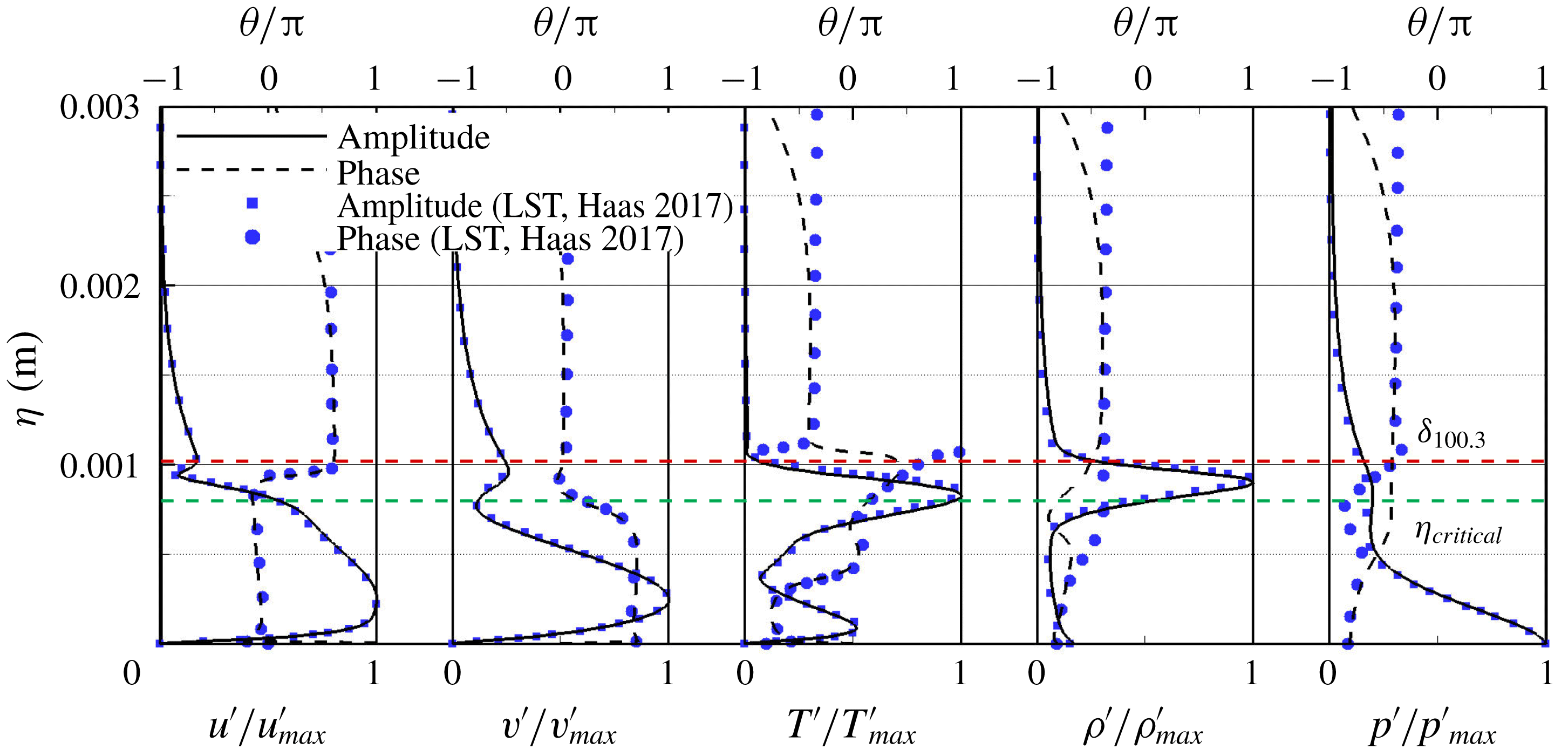
. The normalized amplitude and phase distributions, as shown in figure 14, are used for the time-dependent inflow boundary condition. They were obtained from the low amplitude axisymmetric pulse calculations as discussed in § 6.1. The amplitude and phase distributions from the low amplitude pulse calculation are in good agreement with those calculated using compressible LST (A. P. Haas, private communication 2017) using the re-converged base-flow profiles obtained in step 2 (§ 2). Note, that for the compressible LST analysis the streamwise curvature terms were neglected. The good agreement between the LST results and the wall-normal amplitude and phase distributions in figure 14 suggests that the streamwise curvature has only a small effect in the LST analysis. The inflow boundary for the secondary instability calculations was located at
 $x=0.15~\text{m}$
because this is close to the location where the primary disturbance wave frequency (
 $f_{(1,0)}=300~\text{kHz}$
) is amplified (see figure 13
b). This avoids having to compute through large parts of the boundary-layer flow that are linearly stable. Thus, the computational resources could be focused on parts of the flow field that are relevant for the nonlinear breakdown.
The secondary wave disturbances are introduced through a blowing and suction slot by prescribing a wall-normal velocity disturbance (figure 5
a) with a forcing amplitude of
 $A_{(1,\pm 1)}=A_{(1/2,\pm 1)}=10^{-5}$
. As discussed regarding the forcing location for the primary instability calculations, the forcing slot for the secondary instability calculations is also located 100 grid points downstream of the inflow boundary to avoid possible reflections of the disturbance waves that travel upstream.
Wall-normal amplitude and phase distributions obtained with a low amplitude pulse simulation and eigenfunctions from compressible LST (A. P. Haas, private communication 2017).

The initial forcing amplitudes of the primary and secondary disturbance wave for the secondary instability calculations (
 $A_{(1,0)},A_{(1,1)}$
) were selected based on calculations where for a fixed
 $k_{c,(1,1)}=80$
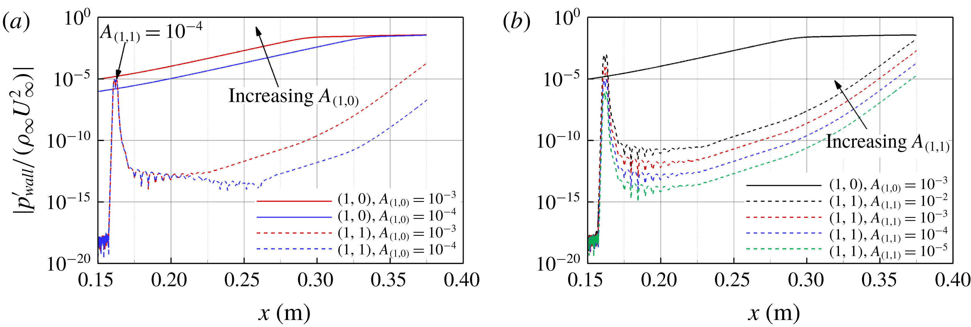
first the primary disturbance wave amplitude and then the secondary wave amplitude was varied while the other remained at a fixed value. The fundamental resonance onset for two different primary wave forcing amplitudes is provided in figure 15(a). Based on these results the initial amplitude was chosen as
 $A_{(1,0)}=10^{-3}$
in order to obtain a ‘clean’ resonating behaviour within the computational domain. With the primary wave amplitude fixed at
 $A_{(1,0)}=10^{-3}$
the amplitude development in the downstream direction for several secondary disturbance amplitudes is shown in figure 15(b), which indicates that the results are less sensitive to the initial forcing amplitude of the secondary wave. To isolate the secondary instability behaviour (interaction between modes (
 $1,0$
) and (
 $1,1$
)) the secondary disturbance wave amplitude was selected to be
 $A_{(1,1)}=10^{-5}$
.
Fundamental resonance onset for a test case with
 $k_{c,(1,1)}=80$
for (a) a varying primary wave forcing amplitude with
 $A_{(1,1)}=10^{-4}$
, and for a (b) varying secondary wave forcing amplitude with
 $A_{(1,0)}=10^{-3}$
.

To determine which azimuthal wavenumber (
 $k_{c}$
) leads to the strongest onset of either the fundamental or the subharmonic resonance, ‘low-resolution simulations’ (resolution is low compared to the resolution that would be needed for later nonlinear stages and breakdown, but it is sufficient for secondary instability investigations) were carried out for both scenarios. Details of the computational set-up are provided in table 4.
Fundamental and subharmonic resonance onset simulation set-up.

The azimuthal wavenumber,
 $k_{c}$
, of the respective resonance scenarios can be varied by adjusting the extent of the azimuthal domain (
 $\unicode[STIX]{x1D711}_{domain}$
, figure 5). Typical results from low-resolution simulations of a fundamental and subharmonic resonance onset (
 $k_{c}=80$
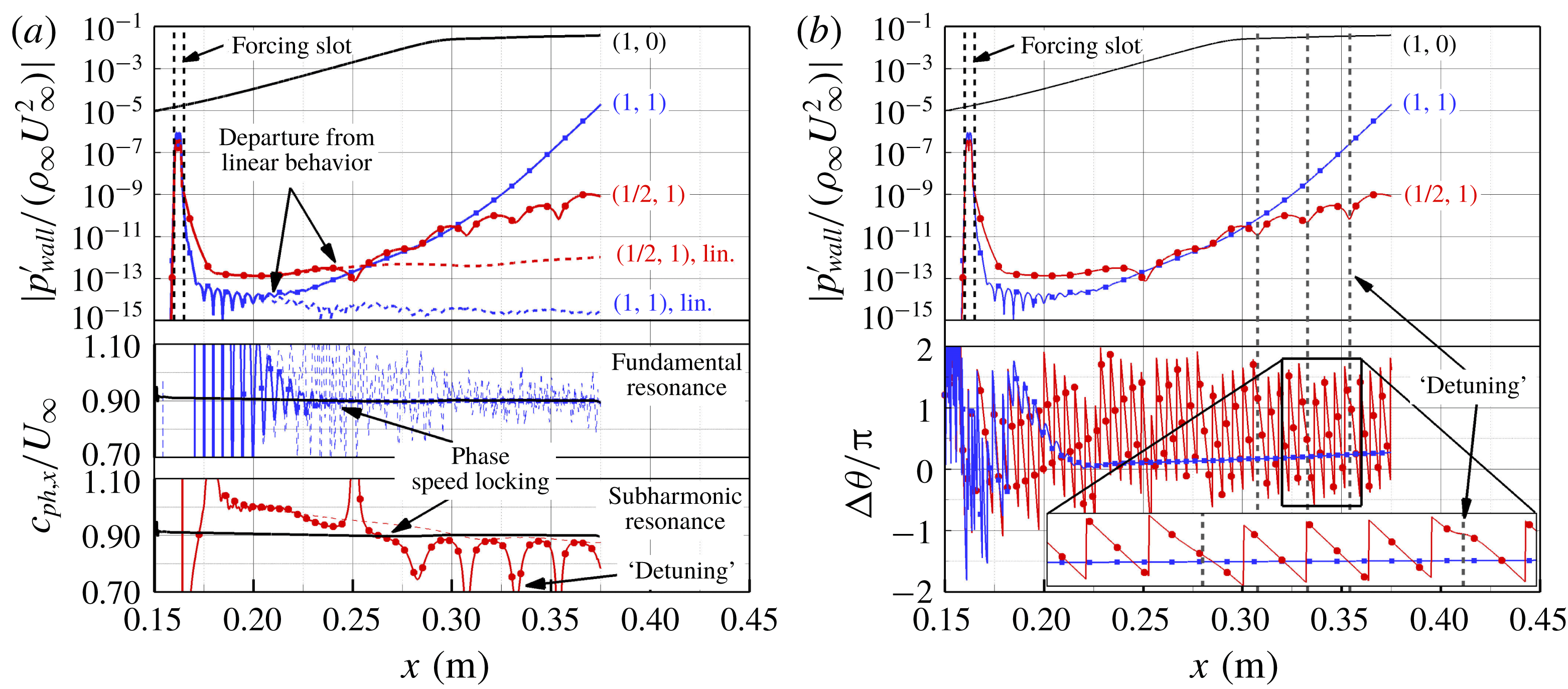
) are provided in figure 16. The wall pressure disturbance amplitude and phase speed development in the streamwise direction are plotted in figure 16(a). For reference, the ‘linear’ behaviour of the secondary wave is also plotted in figure 16(a), which in this context refers to the amplitude development of the secondary wave if the large amplitude primary wave were not present. As can be observed in figure 16(a) (top), the primary wave grows exponentially until it reaches a large enough amplitude and then begins to saturate. As the primary wave saturates, a phase speed locking process occurs between the primary and the secondary waves (figure 16(a), middle: fundamental resonance, bottom: subharmonic resonance) and then the growth of the secondary wave begins to deviate from its ‘linear’ behaviour due to the secondary instability mechanism. The comparison between the fundamental and subharmonic resonance cases in figure 16(a) indicates that for this particular azimuthal wavenumber the secondary instability onset is significantly stronger for the fundamental than for the subharmonic resonance. Once the phase speeds of the primary and secondary waves are ‘locked’ in (figure 16(a), middle: fundamental resonance, bottom: subharmonic resonance), the secondary wave experiences strong exponential growth, which is consistent with secondary linear stability theory (Herbert Reference Herbert1988). For the subharmonic resonance, the phase speed of the secondary wave appears to be alternately ‘locked’ and ‘detuned’ with the phase speed of the primary wave, which ultimately leads to a weaker resonance in this case. This ‘detuning’ can be explained by consulting the phase difference,
 $\unicode[STIX]{x0394}\unicode[STIX]{x1D703}$
, between the primary and the secondary disturbance wave in figure 16(b) (bottom). According to Herbert (Reference Herbert1988), synchronization between primary and secondary waves provides an optimum chance for the transfer of energy into the secondary disturbance wave. The waves are considered synchronized when they are phase locked and propagate at the same phase speed. In the fundamental resonance scenario, the phase difference between the two waves assumes a nearly constant value, whereas for the subharmonic resonance the phase difference between the two waves varies strongly. At the locations where the waves are detuned, a strong modulation in the phase difference can be observed. As a consequence, the primary and secondary wave are alternately either phase locked or out of phase, leading to an alternation of optimal and non-optimal conditions for energy exchange and therefore for resonance for the subharmonic case.
Typical results from low-resolution fundamental and subharmonic resonance simulations (
 $k_{c}=80$
,
 $f_{(1,0)}=f_{(1,1)}=300~\text{kHz}$
,
 $f_{1/2,1}=150~\text{kHz}$
). Wall pressure disturbance amplitude (top) and streamwise phase speed development in the downstream direction (middle: fundamental resonance, bottom: subharmonic resonance) (a), and wall pressure disturbance amplitude (top) and phase difference (bottom) between the primary and the secondary disturbance wave (b).

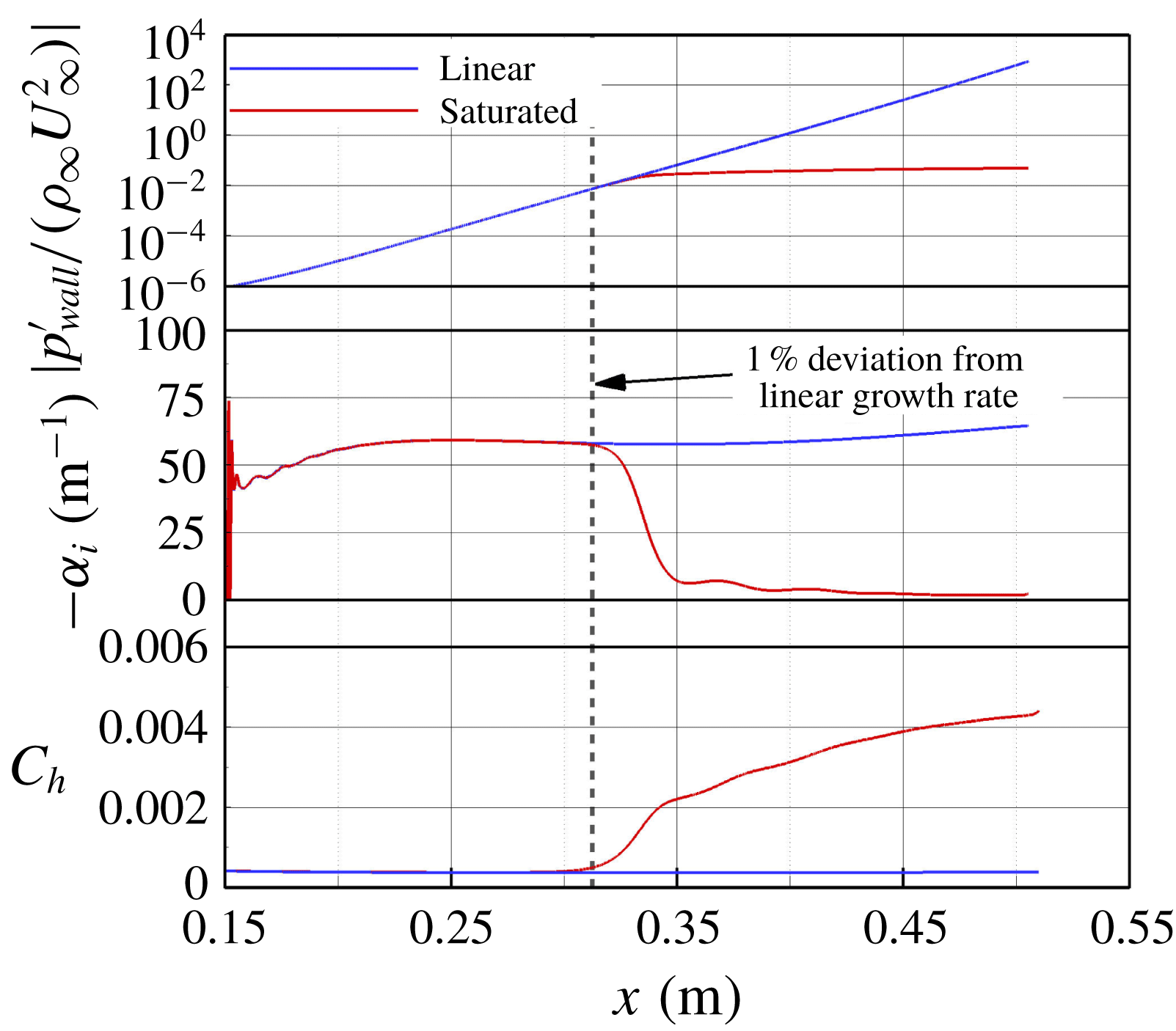
The wall pressure disturbance amplitude, the spatial growth rate development of the primary wave and the Stanton number development for a linear and saturated case are compared in figure 17. When the primary wave begins to saturate, its spatial growth rate drops rapidly, and the Stanton number begins to deviate from its laminar value (figure 17). A small deviation (1 %) of the spatial growth rate from its linear value indicates that the primary wave is beginning to saturate, which coincides with the location where the Stanton number begins to rise. The location where the Stanton number begins to deviate from the laminar values is often defined as the transition onset location (see for example Balakumar & Chou Reference Balakumar and Chou2016). The growth rate of the secondary instability waves is dependent on the spanwise wavenumber
 $k_{c}$
. Therefore, the low-resolution simulations were carried out for both the fundamental and the subharmonic resonance for a range of azimuthal wave numbers from
 $k_{c}=5$
to
 $k_{c}=200$
in increments of
 $\unicode[STIX]{x0394}k_{c}=5$
. Furthermore, the strength of the resonance onset is dependent on the
 $N$
-factors of the secondary disturbance waves, which were calculated in the same manner as for the primary waves as discussed in § 6.1.
Wall pressure disturbance amplitude development, spatial growth rate development in the streamwise direction for the primary wave and the Stanton number development for a linear and a saturated case.

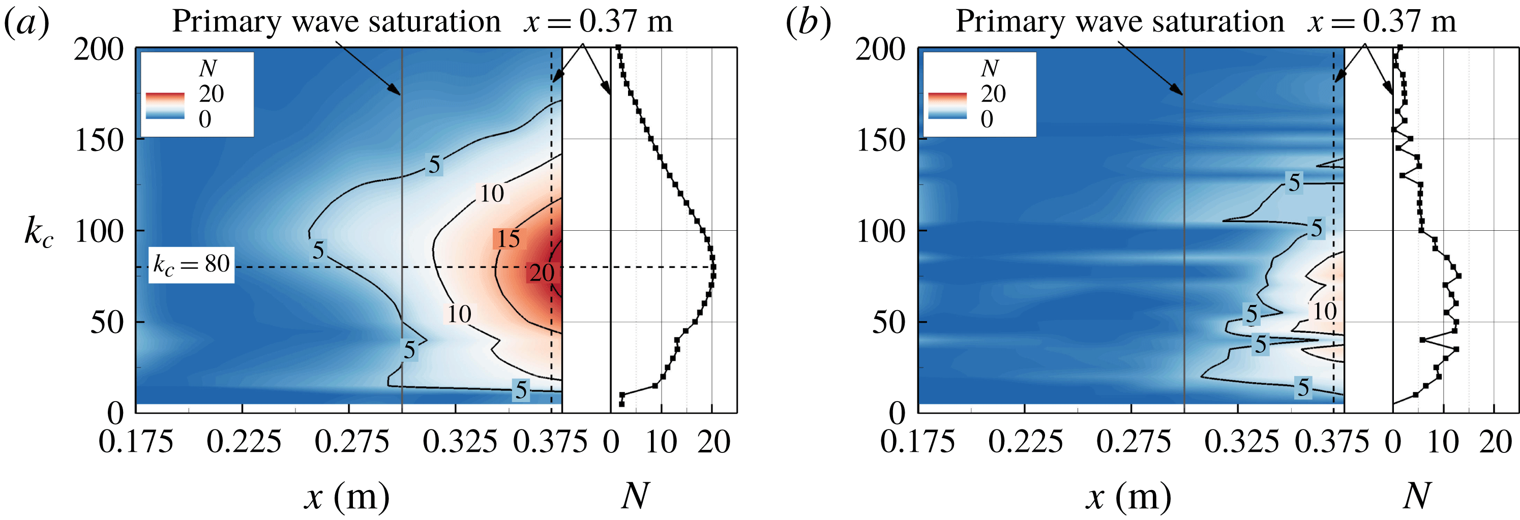
The
 $N$
-factor contours in figure 18 reveal for which wavenumbers the secondary disturbance waves have grown the most in an integral sense. Comparing the results obtained for the fundamental resonance (figure 18
a) and the subharmonic resonance (figure 18
b) indicates that the fundamental resonance is much stronger as it leads to much larger
 $N$
-factors. This is consistent with the findings of Li et al. (Reference Li, Choudhari, Chang and White2012). A direct comparison of the
 $N$
-factors versus the azimuthal wavenumber (for example, at a fixed downstream location of
 $x=0.37~\text{m}$
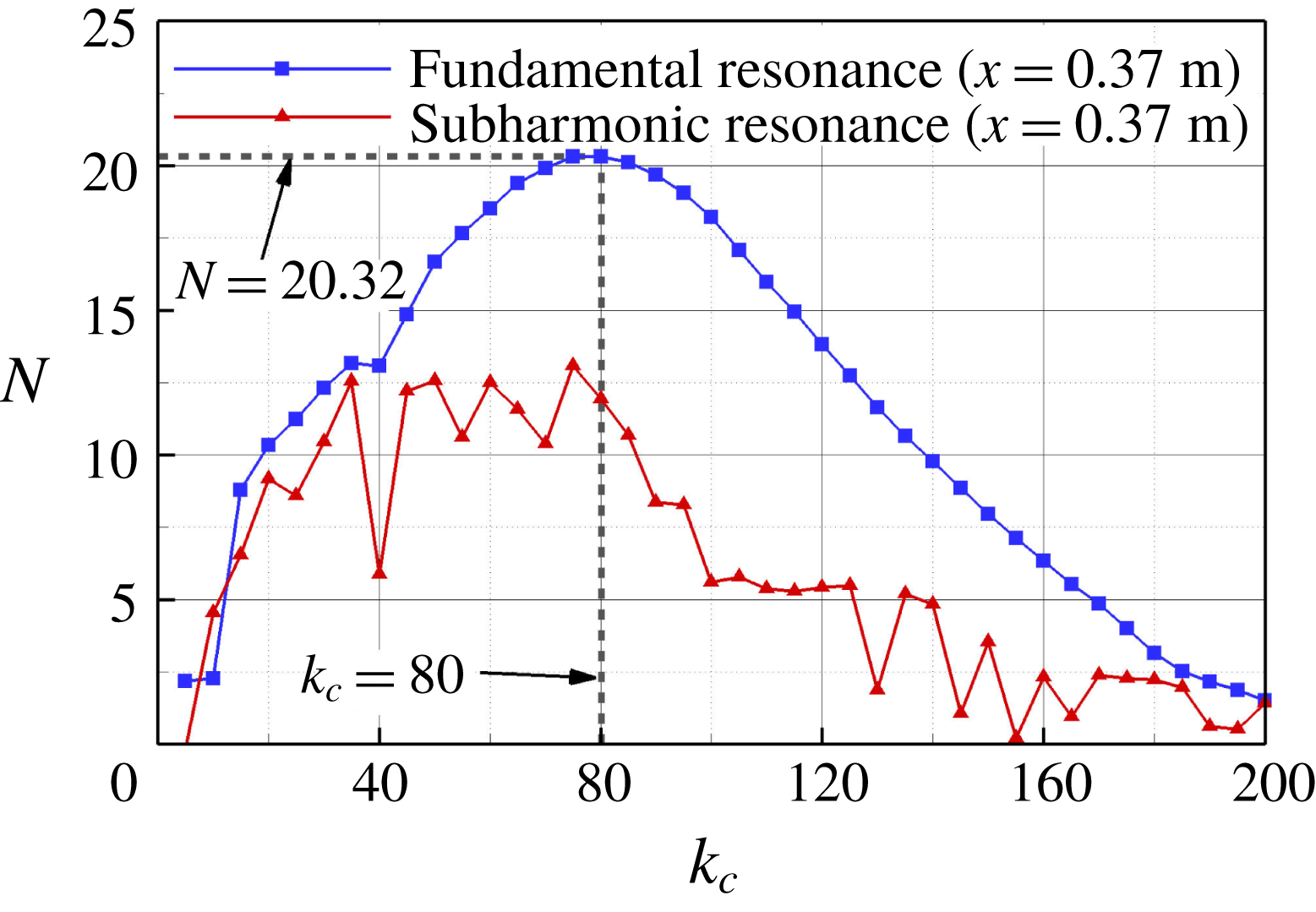
) between the two resonance scenarios is provided in figure 19 and reveals that the azimuthal wavenumber
 $k_{c}=80$
leads to the largest
 $N$
-factor for the fundamental resonance. The distribution of the
 $N$
-factor in azimuthal wavenumber space extracted at
 $x=0.37$
(figure 19) appears to be much ‘noisier’ for the subharmonic compared to the fundamental resonance. This can be attributed to the ‘detuning’ process shown in figure 16(b). In addition, the data were not smoothed in azimuthal wavenumbers space.
 $N$
-factors of the secondary disturbance wave in the downstream direction for varying azimuthal wavenumbers (
 $k_{c}$
) for the fundamental resonance (a), and the subharmonic resonance onset (b).

Based on the results provided here the fundamental resonance is the much more likely scenario to lead to transition than the subharmonic resonance for the flow conditions considered here and will therefore be subject of the high-resolution breakdown simulations discussed below in § 6.3. Under the assumption that the fundamental breakdown with a secondary wave resulting in the largest secondary
 $N$
-factor would prevail in the breakdown for the BAM6QT experimental conditions, the azimuthal wavenumber
 $k_{c}=80$
was chosen for the secondary wave, (
 $1,\pm 1$
), for the fundamental breakdown simulation (§ 6.3).
Comparison of the
 $N$
-factors of the secondary waves after resonance onset extracted at
 $x=0.37~\text{m}$
.

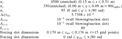
Parameters for the high-resolution fundamental breakdown simulation.

6.3 Fundamental breakdown simulations
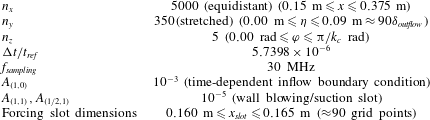
The spatial resolution chosen for the high-resolution fundamental breakdown simulations is based on our previous experience (see Laible Reference Laible2011; Terwilliger Reference Terwilliger2011; Fasel et al. Reference Fasel, Sivasubramanian and Laible2015; Sivasubramanian & Fasel Reference Sivasubramanian and Fasel2015). The computational parameters used are provided in table 5.
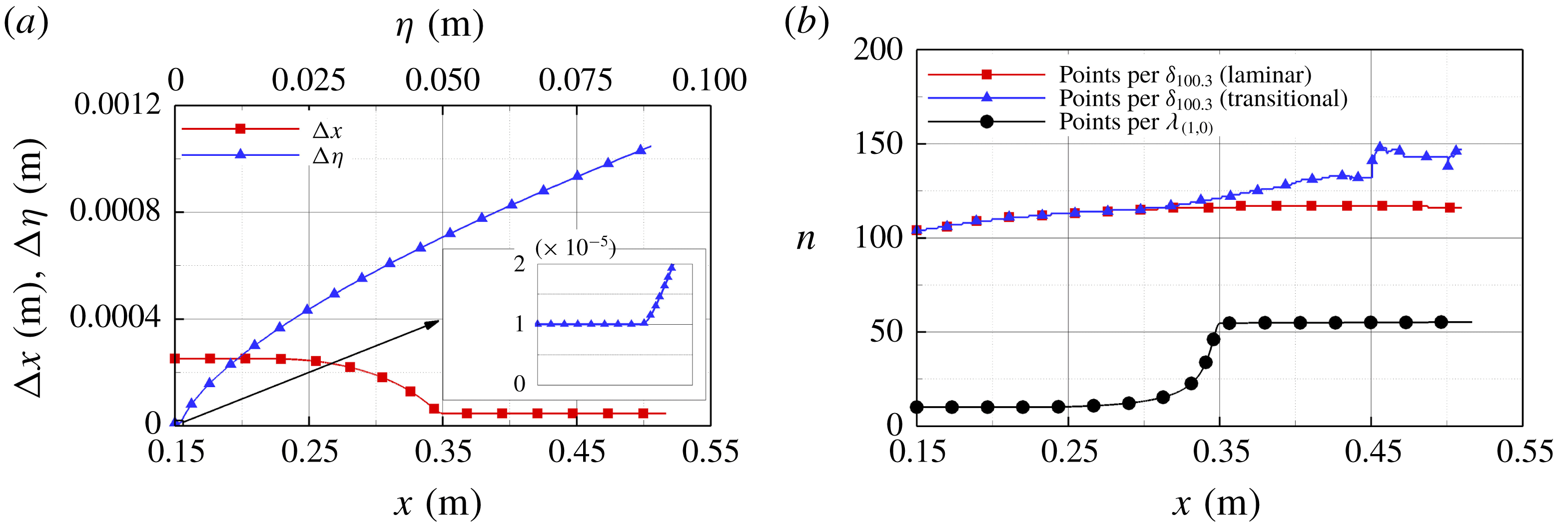
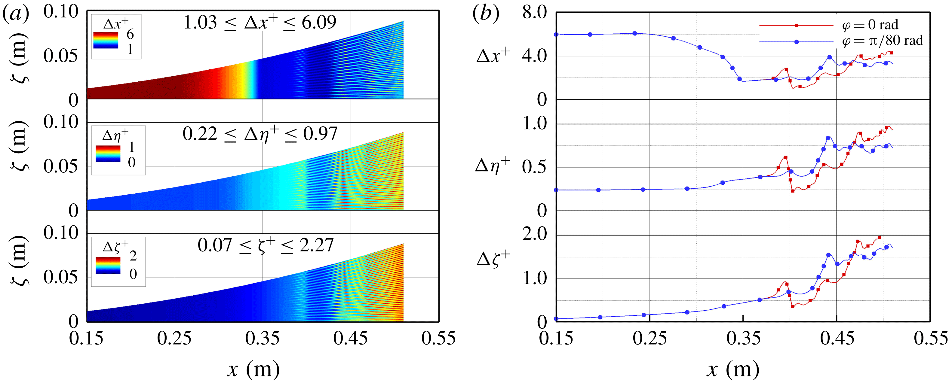
The streamwise and wall-normal grid-density functions are shown in figure 20(a). In the streamwise direction the grid spacing is initially equidistant and then refined towards the downstream end of the computational domain in order to resolve the highly nonlinear stages and the breakdown region. In the wall-normal direction, the grid-line spacing near the wall is equidistant (
 $\unicode[STIX]{x0394}\unicode[STIX]{x1D702}_{wall}=10^{-5}~\text{m}$
) at first and then stretched towards the free stream. The number of points per boundary-layer thickness (figure 20
b) was calculated for the laminar base flow and the time-averaged modified (transitional) base flow from the fundamental breakdown simulation. Throughout the domain the boundary layer is resolved with approximately 100 points in the wall-normal direction which is deemed to be sufficient considering the high-order accuracy of the numerical method. Once the flow begins to transition the boundary layer becomes thicker and the transitional boundary layer is consequently resolved with more points. To assess the quality of the streamwise resolution, the number of points per primary wavelength is plotted in figure 20(b). At the beginning of the computational domain the primary wave is resolved with approximately 15 points per wavelength and with approximately 55 points per wavelength in the refined region further downstream.
Grid-density functions in the streamwise and the wall-normal directions (a), and points per boundary-layer thickness (100.3 % total enthalpy criterion) and points per primary wavelength at each downstream location (b).

To initiate the fundamental breakdown (figure 10
a), the primary wave, (
 $1,0$
), and the secondary wave, (
 $1,1$
), were forced with initial amplitudes of
 $A_{(1,0)}=10^{-4}$
and
 $A_{(1,1)}=10^{-2}$
, respectively, as wall-normal velocity disturbances through a wall blowing and suction slot (figure 5
a). Using a higher initial forcing amplitude for the secondary wave than for the primary wave is justified by examining figure 16(a), which exhibits a sharp decrease of the wall pressure disturbance amplitude of the oblique secondary waves, (
 $1,1$
) and (
 $1/2,1$
), immediately downstream of the forcing location. Thus, the amplitude, for which these waves are effectively seeded into the flow is several orders of magnitude lower compared to their initial forcing amplitudes. This drop from the initial to the ‘effective’ amplitude is much less pronounced for the two-dimensional primary wave. Consequently, even though
 $A_{(1,0)}<A_{(1,1)}$
, the ‘effective’ amplitude of the primary wave is much larger than that of the secondary wave due to the fact that the boundary layer is much more receptive with respect to two-dimensional disturbance waves compared to the highly oblique secondary disturbance waves. Therefore, for the present simulations the fundamental breakdown is effectively initiated by a large amplitude primary wave and a small amplitude secondary wave as would be required for a fundamental (
 $K$
-type) resonance (figure 10
a).
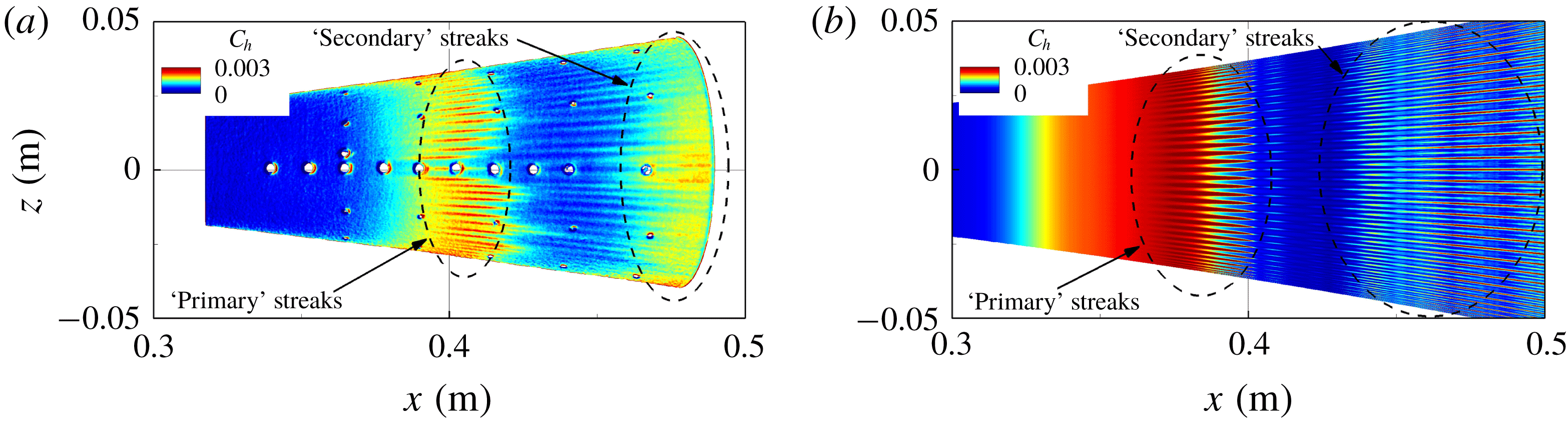
The temperature sensitive paint (TSP) image from the experiments at the BAM6QT facility (B. C. Chynoweth, personal communication 2017) in figure 21(a) was obtained for similar flow conditions (
 $p_{0}=141.3~\text{psi}$
,
 $T_{0}=429.5~\text{K}$
) as the ones used for the present ‘controlled’ fundamental breakdown DNS (
 $p_{0}=140~\text{psi}$
,
 $T_{0}=420~\text{K}$
). A comparison of Stanton number contours obtained from the experiment (figure 21
a) with the time-averaged Stanton number contours on the surface of the cone from the ‘controlled’ breakdown DNS (figure 21
b) reveals qualitatively similar patterns of streamwise streaks. For both the experimental and the DNS results, the TSP contours and the time-averaged Stanton number contours are uniform until ‘hot’ streaks appear. These ‘hot’ streaks then disappear before reappearing further downstream. To distinguish the two streak patterns, the streaks that appear first will be referred to as ‘primary’ and the reappearing streaks as ‘secondary’ streaks in the following discussion. For reference, the approximate start and end of the ‘primary’ streaks (
 $x_{primary,start}\approx 0.38~\text{m}$
,
 $x_{primary,end}\approx 0.40~\text{m}$
) and the beginning of the ‘secondary’ streaks (
 $x_{secondary,start}\approx 0.42~\text{m}$
) were determined from the Stanton number contours in figure 21(b). Of course the determination of the start and end of the streaks depends on the choice of the contour levels and is therefore not an accurate measure. It is nonetheless informative to highlight these locations to indicate where different effects can be observed relative to the streak locations.
The similarities of the patterns between the experiments and the DNS in figure 21 are an indication that the ‘controlled’ fundamental breakdown captures the nonlinear transition stages for the BAM6QT flared cone experiments. In particular, it appears that the streak development in the experiments is indeed due to a fundamental breakdown. To provide convincing evidence that this is the case, in the following the DNS results are examined in great detail.
Streak patterns observed on the surface of the flared cone obtained in the experiments carried out at Purdue University (
 $p_{0}=141.3$
psi and
 $T_{0}=419.5$
K, B. C. Chynoweth, personal communication 2017) using TSP (a), and with DNS (
 $p_{0}=140~\text{psi}$
,
 $T_{0}=420~\text{K}$
) (b).

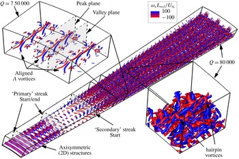
The instantaneous flow structures of the fundamental breakdown simulation are visualized in figure 22 using
 $Q$
-isocontours coloured with the streamwise vorticity values. The data are extended periodically in the azimuthal direction for illustration purposes. For reference, the start and end of the ‘primary’ streaks and the beginning of the ‘secondary’ streaks, which were found approximately from the Stanton number contours in figure 21(b), are also provided in figure 22.
The
 $Q$
-isocontours reveal in figure 22 that upstream of the ‘primary’ streak onset the flow is dominated by two-dimensional (axisymmetric) structures (due to large amplitude 2-D second-mode waves). In the primary streak region, the structures are periodically modulated in the azimuthal direction with the azimuthal wavenumber of the secondary instability waves. In between the ‘primary’ and ‘secondary’ streaks, a ‘quiet’ zone can be observed where the vortical structures exhibit a significantly reduced intensity compared to the ‘primary’ and ‘secondary’ streak regions.
The close up in the upper left corner of figure 22 (using different isocontour levels) exposes aligned
 $\unicode[STIX]{x1D6EC}$
vortices that are typical for a
 $K$
-type breakdown. The streamwise vorticity contours show that the ‘legs’ of the
 $\unicode[STIX]{x1D6EC}$
vortices are counter rotating. The close-up also indicates the so-called peak and valley planes (wall-normal planes) through the tip and the legs of the
 $\unicode[STIX]{x1D6EC}$
vortices, respectively.
The other close up in the lower right-hand corner of figure 22 displays the hairpin vortices that are generated when the
 $\unicode[STIX]{x1D6EC}$
vortices begin to break down due to tertiary instabilities (see Klebanoff et al.
Reference Klebanoff, Tidstrom and Sargent1962).
Visualization of the instantaneous flow structures of the fundamental breakdown using the
 $Q$
-criterion. The
 $Q$
-isosurfaces are coloured by the streamwise vorticity.

In experiments, schlieren imaging techniques have been successfully employed to visualize the instability phenomena and transition in hypersonic boundary layers (see for example Casper et al.
Reference Casper, Beresh, Henfling, Spillers and Pruett2013a
,Reference Casper, Beresh, Wagnild, Henfling, Spillers and Pruett
b
; Laurence et al.
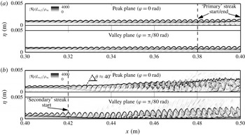
Reference Laurence, Wagner, Ozawa and Hannemann2014). To obtain qualitatively comparable images from DNS data to experimental schlieren the magnitude of the instantaneous total density gradient (‘pseudo-schlieren’) can be used as shown in figure 23. The numerical schlieren visualization of the flow field in the peak and the valley planes for the downstream extent from
 $x=0.3~\text{m}$
to
 $x=0.4~\text{m}$
(figure 23
a) and from
 $x=0.4~\text{m}$
to
 $x=0.5~\text{m}$
(figure 23
b) shows the typical characteristics of a transitional boundary layer that have been observed in experiments. In figure 23(a) rope-like structures are developing at the edge of the boundary layer, which have been identified as being typical for second mode waves (see for example Laurence et al.
Reference Laurence, Wagner, Ozawa and Hannemann2014). Further downstream, the well-organized rope-like structures begin to contain smaller and smaller scales (figure 23
b) as the boundary layer progresses deeper into the nonlinear breakdown regime. In the peak plane, the breakdown into smaller scales occurs away from to wall whereas in the valley plane the development of smaller structures occurs close to the wall. Mach waves can be observed that are radiated from the transitional boundary layer in the peak plane. The angle of these Mach waves is approximately
 $40^{\circ }$
, which is close to the angle of the Mach waves radiated from the turbulent boundary layer for the BAM6QT conditions on a flat plate (
 $30^{\circ }$
) geometry as reported by Duan, Choudhari & Zhang (Reference Duan, Choudhari and Zhang2016). The difference in Mach wave angle between the value found by Duan et al. (Reference Duan, Choudhari and Zhang2016) and the wave angle obtained with the DNS results here can be attributed to the difference in geometry (e.g. the strong streamwise adverse pressure gradient for the flared cone). Note that from figure 23 the ‘primary’ and ‘secondary’ streak region could not be identified as no drastic changes can be observed in these regions. The approximate locations of the ‘primary’ and ‘secondary’ streak onset and end are marked with vertical dashed lines.
Contours of the magnitude of the density gradient (‘pseudo-schlieren’) in the peak and valley plane for
 $0.3~\text{m}\leqslant x\leqslant 0.4~\text{m}$
(a) and
 $0.4~\text{m}\leqslant x\leqslant 0.5~\text{m}$
(b).

The density magnitude contours extracted at various wall-normal distances from the cone surface in the planes parallel to the cone surface and unrolled in the azimuthal direction are displayed in figure 24. Note that for figure 24 the unrolled coordinate was calculated with the local radius measured from the cone axis to the point in the flow field as indicated in figure 7(d), and not by using the local cone radius,
 $r_{cone}(x)$
. In this view, for a distance closest to the wall (
 $\unicode[STIX]{x1D702}/\unicode[STIX]{x1D6FF}_{laminar}\approx 0.20$
) the presence of the ‘primary’ and ‘secondary’ streak regions can be identified because distinctly different streamwise structures can be observed in the ‘primary’ streak region, in the ‘quiet’ region between the ‘primary’ and ‘secondary’ streaks and then again at the onset of the ‘secondary’ streaks. Comparing the contour plots for different wall distances reveals that generally the breakdown to small scales occurs much closer to the wall in the valley plane compared to the peak plane, which is consistent with the observations made in figure 23 that the small scale structure development is pushed towards the wall in the valley plane. Further away from the wall (
 $\unicode[STIX]{x1D702}/\unicode[STIX]{x1D6FF}_{laminar}\approx 0.42$
) the three-dimensional ‘wedge-like’ structures begin to appear further upstream, before the ‘secondary’ streaks appear, compared to the plane closer to the wall where these structures are observed after the ‘secondary’ streaks have formed. At
 $\unicode[STIX]{x1D702}/\unicode[STIX]{x1D6FF}_{laminar}\approx 0.63$
and
 $\unicode[STIX]{x1D702}/\unicode[STIX]{x1D6FF}_{laminar}\approx 0.85$
the breakdown from two-dimensional to three-dimensional structures is moved upstream compared to the planes lower in the boundary layer. The ‘pseudo-schlieren’ images confirm that before the ‘primary’ streaks appear, the flow is dominated by axisymmetric waves as was observed also from the
 $Q$
-isocontours in figure 22. Close to the end of the ‘primary’ streaks the structures exhibit a modulation in the azimuthal direction, corresponding to the azimuthal wavenumber of the secondary disturbance wave, and over a short downstream distance the dominant two-dimensional character of the disturbances quickly disappears.
Contours of the magnitude of the density gradient in the unrolled
 $x$
–
 $\unicode[STIX]{x1D701}$
planes extracted at different distances from the cone surface.

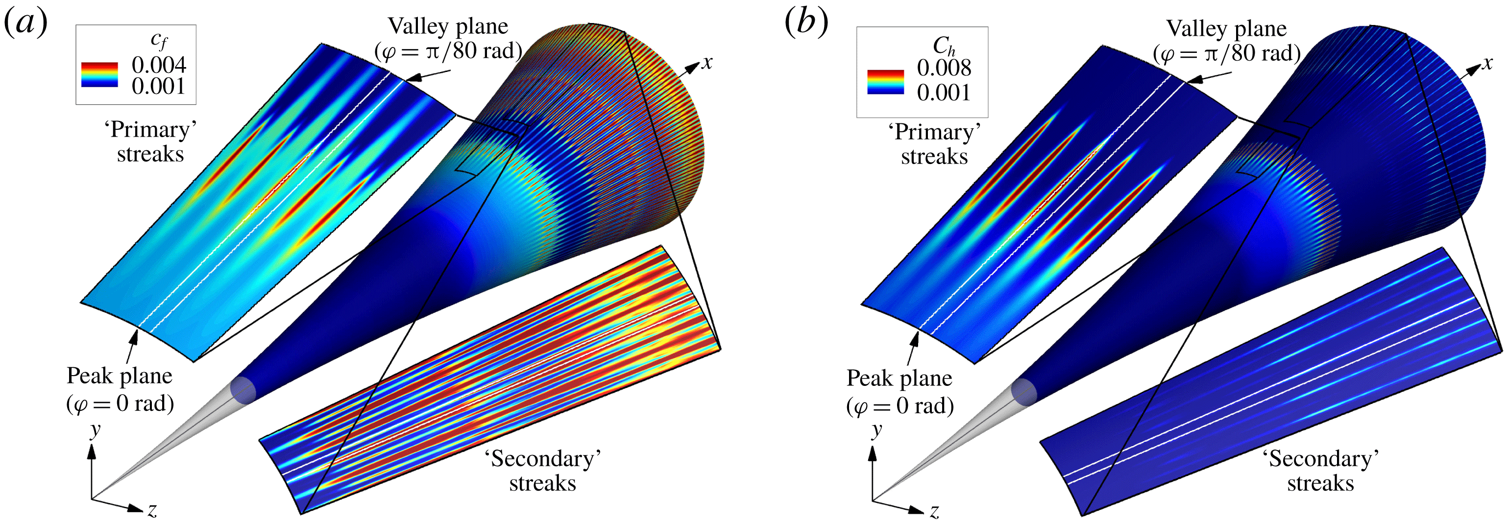
To shed light on the development of the streamwise streaks on the cone surface, the DNS data are averaged in time (arithmetic average). The time-averaged skin-friction coefficient and the time-averaged Stanton number on the surface of the cone are shown in figure 25(a) and figure 25(b), respectively. Similar patterns of streamwise ‘streaks’ emerge for both quantities. As can be observed in figure 21, the time-averaged skin-friction coefficient and the time-averaged Stanton number are nearly uniform until there is a rise followed by the appearance of ‘primary’ streaks, where locally large skin-friction and Stanton number values are obtained. Both coefficients show little modulation in the azimuthal direction until the ‘primary’ streaks begin to appear. After a limited downstream extent the ‘primary’ streaks disappear and both the skin-friction coefficient and Stanton number drop significantly until a ‘secondary’ streak pattern appears. As can be observed from the colour contour levels, for the time-averaged skin-friction coefficient (figure 25 a) the ‘primary’ streaks are weaker compared to the ‘secondary’ streaks, which indicates that the peak skin-friction coefficient in the secondary peak region is larger compared to the ‘primary’ streak region. The opposite trend is found for the time-averaged Stanton number (figure 25 b) where the ‘primary’ streaks have much higher intensity compared to the ‘secondary’ streaks.
Time-averaged skin-friction coefficient (a), and Stanton number (b) on the surface of the cone.

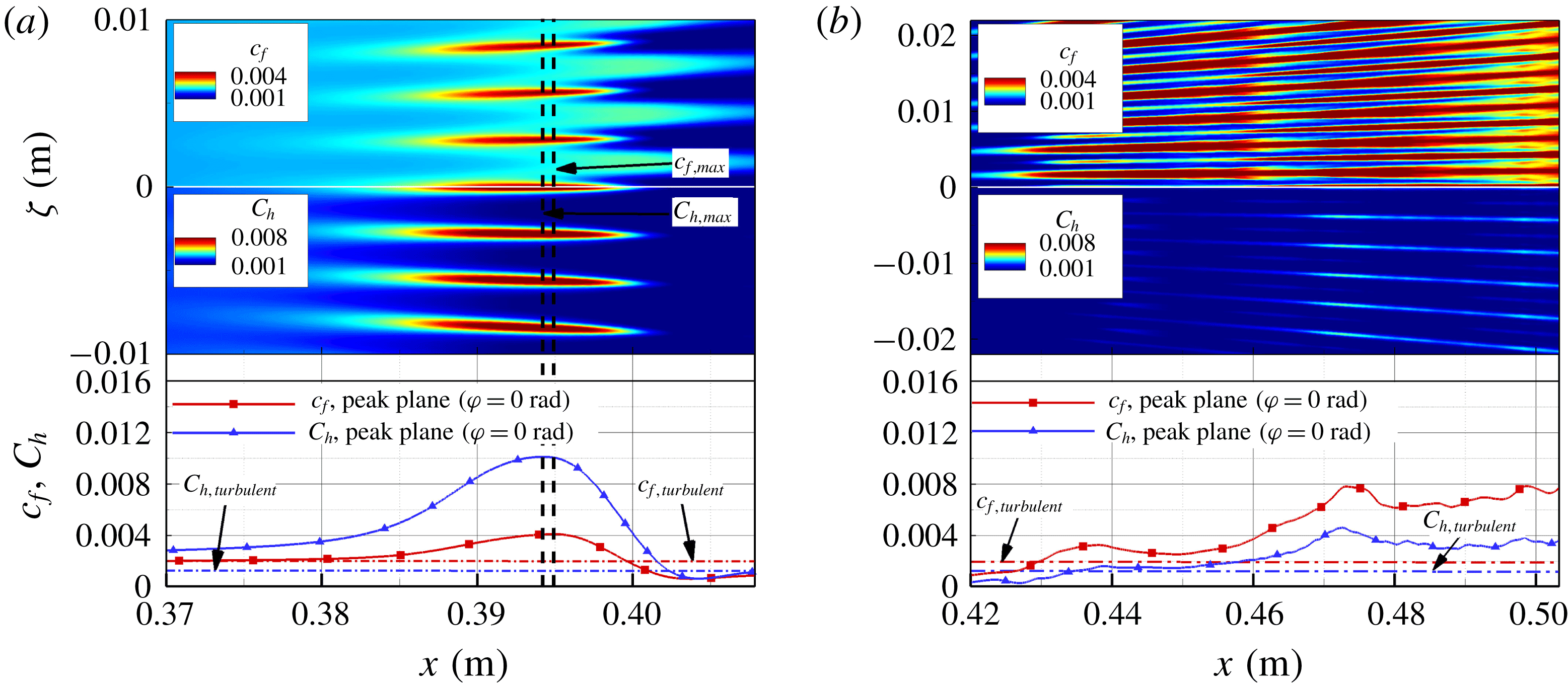
The ‘primary’ streak patterns of the time-averaged skin-friction coefficient and the Stanton number on the unrolled cone surface (see (4.1)) are compared in figure 26(a). The upper half of the cone surface shows the skin-friction coefficient contours and the lower half shows the Stanton number contours. The coefficient development in the streamwise direction through a ‘primary’ streak is provided below the contours. Estimates of the turbulent skin-friction coefficient (
 $c_{f,turbulent}$
) and the turbulent Stanton number (
 $C_{h,turbulent}$
) calculated according to White (Reference White2006) are provided. Note that these theoretical values only provide a qualitative estimate since they were derived for a straight (right) cone geometry, thus neglecting the adverse pressure gradient due to the cone flare. The ‘primary’ streaks appear at the same location and have approximately the same length for both the Stanton number and skin-friction coefficient. The location of the maximum skin-friction coefficient (
 $x=0.3949~\text{m}$
) is nearly identical to the location of the maximum Stanton number (
 $x=0.3942~\text{m}$
). After the ‘primary’ streaks disappear the Stanton number is nearly uniform, whereas the skin-friction coefficient still shows a significant modulation in the azimuthal direction.
The time-averaged contours of the ‘secondary’ streaks on the unrolled cone surface are displayed in figure 26(b), which clearly show how much more intense the ‘secondary’ streaks are when visualized using the skin-friction coefficient compared to the Stanton number. The skin-friction and Stanton number developments in the streamwise direction (bottom figure 26 b) show that both coefficients appear to approach a turbulent value at the end of the computational domain indicating that the flow has progressed deep into the nonlinear breakdown regime.
Close up of the time-averaged skin-friction coefficient and Stanton number on the surface of the ‘primary’ streak region (a), and the ‘secondary’ streak region (b). The turbulent estimates for the skin-friction coefficient (
 $c_{f,turbulent}$
) and the Stanton number (
 $C_{h,turbulent}$
), derived for a straight cone geometry, were calculated according to White (Reference White2006).

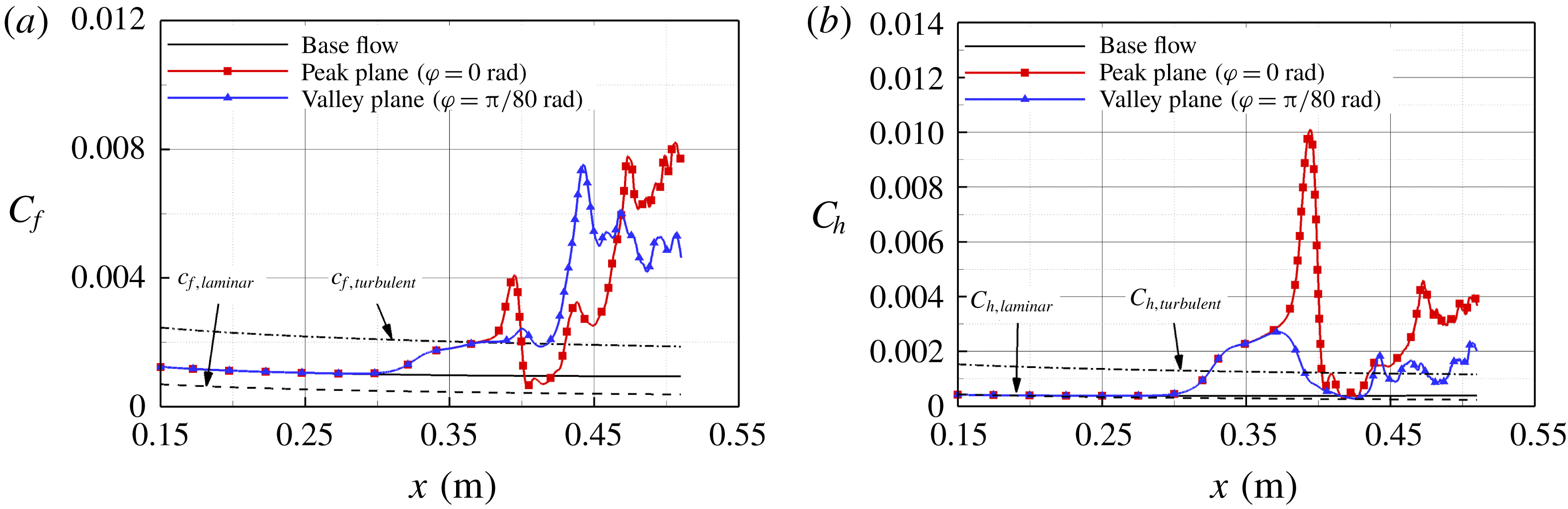
For a more quantitative comparison of the peak values obtained for the ‘primary’ and ‘secondary’ streaks, in figure 27 the time-averaged skin-friction coefficient and Stanton number values are plotted in downstream direction along a ray on the surface of the cone at an azimuthal position that is cutting through a ‘primary’ streak (
 $\unicode[STIX]{x1D711}=0$
rad, see figure 25) and a ray for an azimuthal position in between two ‘primary’ streaks (
 $\unicode[STIX]{x1D711}=\unicode[STIX]{x03C0}/80$
rad, see figure 25). For reference, the base flow values and a laminar and turbulent estimate for a straight cone geometry (White Reference White2006) are provided again in figure 27(a). The skin-friction coefficient begins to depart from its laminar base-flow value at
 $x\approx 0.3$
m. Following that departure is a significant ‘overshoot’ of the turbulent estimate further downstream that is caused by the ‘primary’ streaks before a sharp drop off occurs almost back to the laminar value. After the drop a steep rise towards the turbulent curve follows when the ‘secondary’ streaks begin to appear.
The downstream development of the time-averaged Stanton number along with the laminar base-flow value and the theoretical laminar and turbulent estimates are provided in figure 27(b). Initially it exhibits the same downstream trend as the skin-friction coefficient in figure 27(a). However, the ‘overshoot’ of the turbulent estimate is much larger for the Stanton number compared to the ‘overshoot’ for the skin-friction coefficient.
Downstream development of the time-averaged skin-friction coefficient (a), and Stanton number (b). The laminar and turbulent estimates for the skin-friction coefficient (
 $c_{f,laminar}$
,
 $c_{f,turbulent}$
) and the Stanton number (
 $C_{h,laminar}$
,
 $C_{h,turbulent}$
), derived for a straight cone geometry, were calculated according to White (Reference White2006).

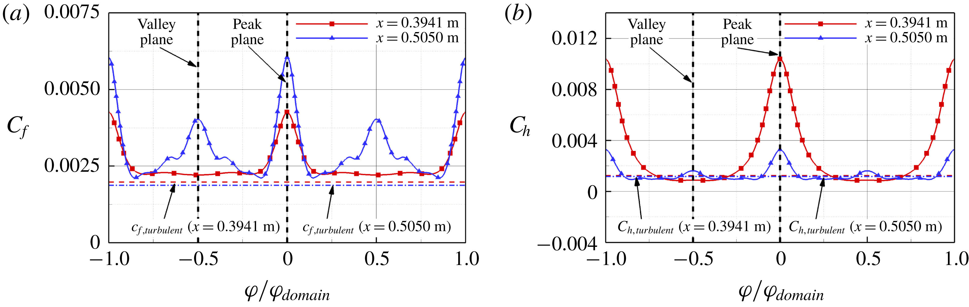
To accurately determine the number of streamwise streaks that arise in the simulation, in figure 28 the time-averaged skin-friction coefficient and the Stanton number are plotted versus the azimuthal direction at a location where the ‘primary’ streaks are present (
 $x=0.3941~\text{m}$
) and at a location where the ‘secondary’ streaks are observed (
 $x=0.5050~\text{m}$
). The azimuthal coordinate is normalized using the azimuthal extent of the domain,
 $\unicode[STIX]{x1D711}_{domain}$
(5.1). The turbulent estimates (White Reference White2006) of the skin-friction coefficient and the Stanton number at the two downstream locations are provided in figure 28 as a qualitative reference. For the fundamental breakdown simulation presented here the azimuthal domain extent was
 $\unicode[STIX]{x1D711}_{domain}=2\unicode[STIX]{x03C0}/80$
, which means that the domain extends over a
 $1/80$
of the cone in the azimuthal direction. The computational domain width determines the smallest azimuthal wavenumber,
 $k_{c,domain}$
(5.1), that can be resolved in the simulation. For better illustration, in figure 28 the data are extended periodically in the azimuthal direction. The skin-friction coefficient in figure 28(a) in the normalized azimuthal direction exhibits a peak exactly one domain width apart at the ‘primary’ streak location (
 $x=0.3941~\text{m}$
). Consequently, there are exactly 80 ‘primary’ streaks around the circumference of the cone at this location. Using the turbulent estimate as a reference at the ‘primary’ streak location reveals a significant overshoot of the turbulent value at the streaks, whereas in between the streaks, good agreement between the turbulent estimate and the time-averaged skin-friction coefficients calculated from the DNS data is found. At the ‘secondary’ streak location (
 $x=0.5050~\text{m}$
) the peaks are spaced exactly half a domain width apart, which means that the streak count has doubled to 160 ‘secondary’ streaks around the circumference of the cone. The Stanton number development in the azimuthal direction in figure 28(b) indicates the same ‘primary’ and ‘secondary’ number of streaks counts as for the skin-friction coefficient.
Variation of time-averaged skin-friction coefficient (a), and Stanton number (b) in the azimuthal direction at a streamwise location where the ‘primary’ streaks are present (
 $x=0.3942~\text{m}$
) and at a location where the ‘secondary’ streaks appear (
 $x=0.5050~\text{m}$
).

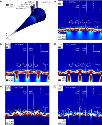
To contribute towards the understanding of the underlying physical mechanisms causing the formation of the streaks, their disappearance and re-appearance further downstream, the time-averaged total flow and the time-averaged disturbance flow fields are plotted in figure 29 for cross-sections at the locations marked in figure 29(a). Here the time-averaged total flow quantities represent the sum of the undisturbed steady laminar base flow and of the time-averaged disturbance flow field (
 $\unicode[STIX]{x1D719}_{total}=\unicode[STIX]{x1D719}_{base}+\unicode[STIX]{x1D719}^{\prime }$
), whereas the disturbance quantities denote the difference between the time-averaged total flow and the undisturbed laminar base flow (
 $\unicode[STIX]{x1D719}^{\prime }=\unicode[STIX]{x1D719}_{total}-\unicode[STIX]{x1D719}_{base}$
). The cross-sections in the wall-normal direction are coloured with isocontours of the time-averaged total temperature contours. In addition, the time-averaged Stanton number contours on the cone surface are also provided in figure 29. Furthermore, streamlines are shown which were generated using the time-averaged disturbance flow field (
 $u^{\prime }$
,
 $v^{\prime }$
,
 $w^{\prime }$
). Time markers, displayed as dots, are seeded at an equidistant
 $\unicode[STIX]{x0394}t$
along the streamlines to indicate how the fluid elements move from one time instance to the next. The laminar boundary-layer thickness of the steady base flow is marked to show where the dominant flow structures are located within the boundary layer.
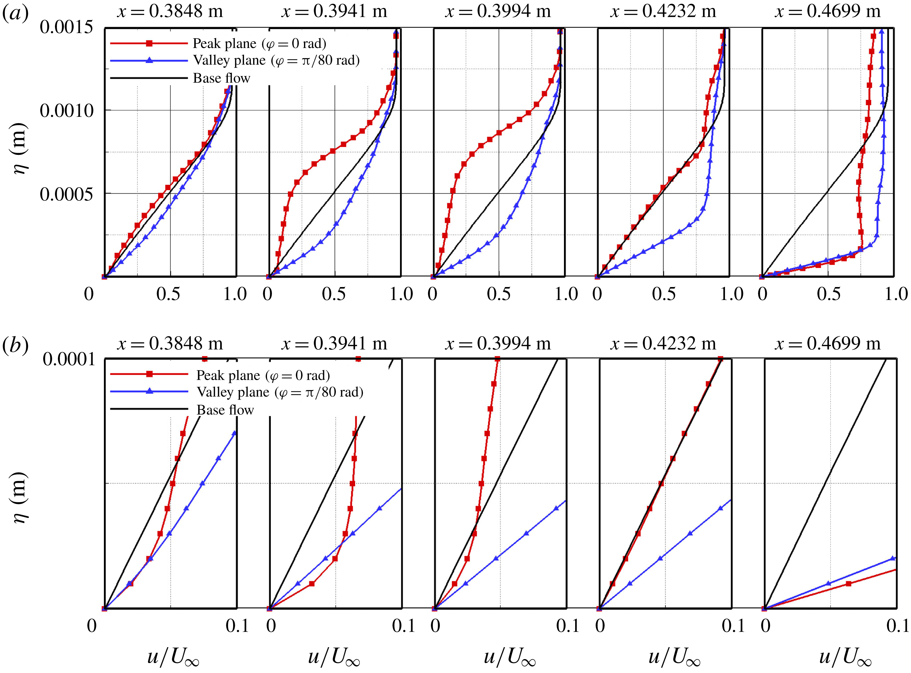
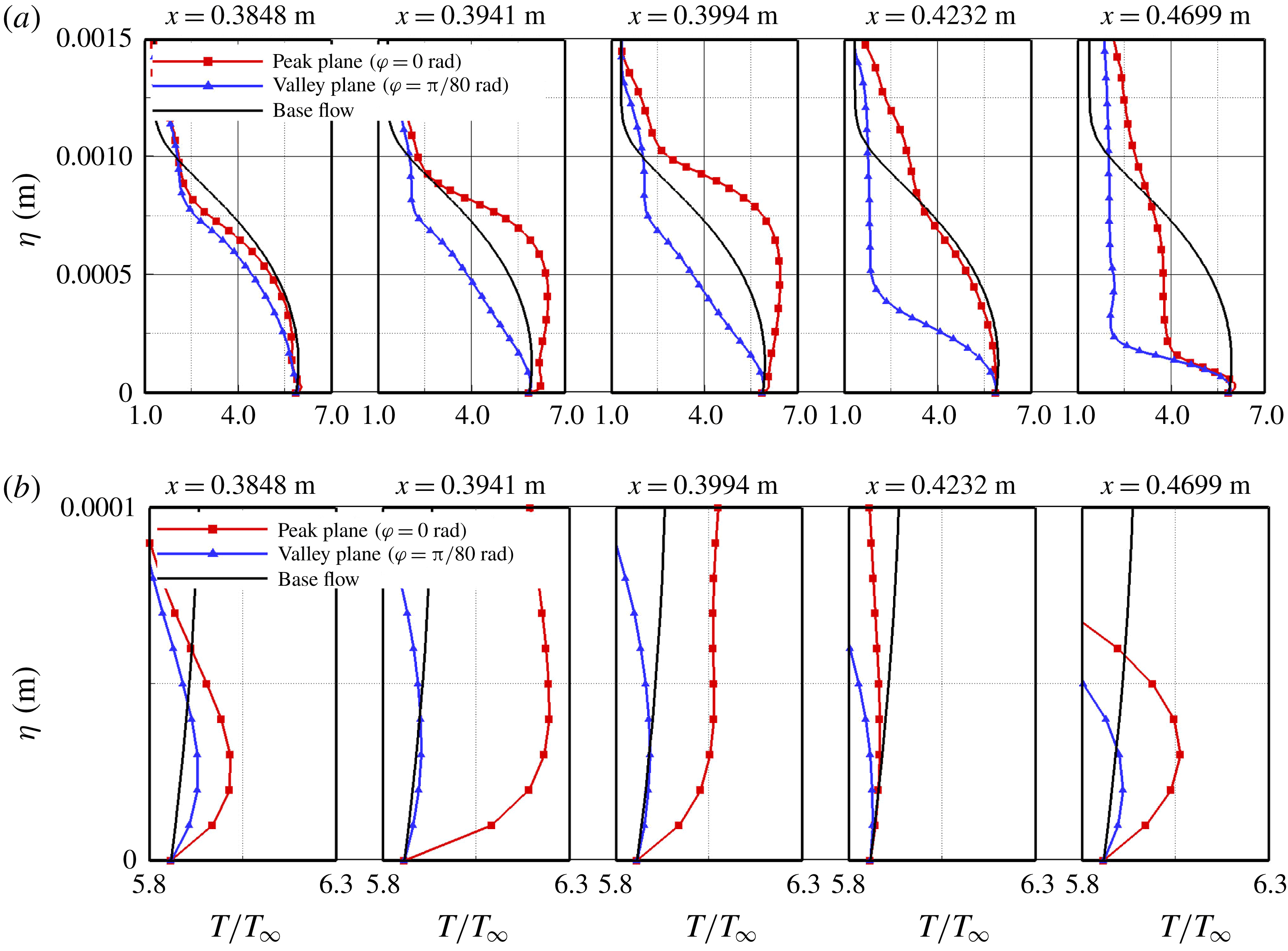
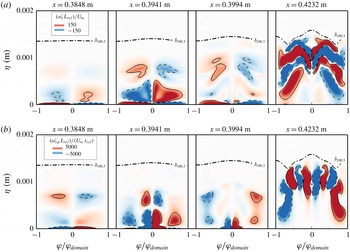
At the location where the ‘primary’ streaks appear (figure 29
b) counter-rotating streamwise vortices are formed. These vortices appear to be confined within the boundary layer. The total temperature contours exhibit a slight modulation in the azimuthal direction. These counter-rotating flow structures entrain ‘cooler’ fluid from the free stream, which is pushed towards the wall and leads to an accumulation of ‘warmer’ fluid above the ‘primary’ streaks. Slightly further downstream at the location where the Stanton number becomes maximal (figure 29
c) the counter-rotating structures are pushed towards the wall. Due to the streamwise vortices ‘warmer’ fluid is accumulating above the ‘primary’ streaks causing the massive overshoot in the Stanton number. In addition, streamlines appear much closer together and the time markers on the streamlines appear to be further apart compared to the previous location. Due to the seeding of these markers at constant time intervals, this indicates that these structures at
 $x=0.3941~\text{m}$
(figure 29
c) rotate faster compared to the location upstream at
 $x=0.3848~\text{m}$
(figure 29
b). At the location, where the ‘primary’ streaks begin to disappear (figure 29
d) the counter-rotating structures are ‘lifted’ away from the wall and the accumulated ‘warmer’ fluid above the streaks appears to be redistributed in such a way that the ‘primary’ streaks are weakened. In the region where the ‘primary’ streaks completely disappear (figure 29
e) the streamwise vortices are completely lifted away from the wall, which explains the decrease of the Stanton number on the surface of the cone back to its laminar value. In addition, smaller secondary structures begin to form indicating that energy is being shifted towards smaller scales and that the flow has progressed into the breakdown regime. In the breakdown region (figure 29
f) the streamwise vortices are pushed back towards the wall, which leads to the formation of the ‘secondary’ streaks. Now it can be observed more clearly that the ‘secondary’ streaks are weaker and that the number has doubled in the breakdown region compared to the ‘primary’ streak location.
Full cone view with time-averaged Stanton number on the surface of the cone with the cross-section planes highlighted (a). Cross-sections showing the time-averaged temperature contours and the streamlines of the disturbance flow field (
 $u^{\prime },v^{\prime },w^{\prime }$
) and the time-averaged Stanton number on the surface of the cone at
 $x=0.3848~\text{m}$
(b),
 $x=0.3941~\text{m}$
(c),
 $x=0.3994~\text{m}$
(d),
 $x=0.4232~\text{m}$
(e) and
 $x=0.4699~\text{m}$
(f).

The rise in the time-averaged skin-friction coefficient and the Stanton number observed in figure 27 must be explainable by an increase of the gradient in the wall-normal direction of the streamwise velocity and the temperature at the wall, respectively. To confirm this, the time-averaged
 $u$
-velocity profiles in the wall-normal direction extracted at select downstream and azimuthal locations are shown in figure 30. The
 $u$
-velocity profiles plotted in figure 30(a) confirm that the increase in skin friction at the ‘primary’ streak (
 $\unicode[STIX]{x1D711}=0$
rad) locations is indeed caused by an increase of the streamwise velocity gradient in a narrow region very close to the wall. A close up of the profiles near the wall in figure 30(b) shows that the rise in the skin friction at the azimuthal location
 $\unicode[STIX]{x1D711}=0$
rad is caused by a small ‘bulge’ in the
 $u$
-velocity profile near the wall (
 $x=0.3848~\text{m}$
,
 $x=0.3941~\text{m}$
,
 $x=0.3994~\text{m}$
). When the bulge disappears the skin-friction coefficient drops back to the laminar value (figure 30(b),
 $x=0.4232$
m). At
 $x=0.4699~\text{m}$
, downstream of the location where the ‘secondary’ streaks appear, the profiles at both azimuthal locations are ‘fuller’ leading to a significant increase in the skin-friction coefficient, which is typical for turbulent flow. This bulge near the wall is not observed for the profiles extracted at an azimuthal location between the ‘primary’ streaks (
 $\unicode[STIX]{x1D711}=\unicode[STIX]{x03C0}/80$
rad), where profiles become gradually fuller resulting in a continuous increase from the laminar to the turbulent skin-friction coefficient without the drop back to the laminar value (see figure 27
a).
The
 $u$
-velocity profiles in the wall-normal direction (
 $\unicode[STIX]{x1D702}$
) of the undisturbed laminar base flow and the time-averaged flow field extracted at an azimuthal location cutting through the ‘primary’ streaks (peak plane,
 $\unicode[STIX]{x1D711}=0$
rad) (a) and in between the ‘primary’ streaks (valley plane,
 $\unicode[STIX]{x1D711}=\unicode[STIX]{x03C0}/80$
rad), and close up of the region near the wall (b).

The time-averaged temperature profiles are plotted in figure 31(a) with the corresponding close ups in figure 31(b). Analogous to the discussion regarding the time-averaged
 $u$
-velocity profiles, the temperature profiles shown in figure 31 confirm that the increase in the Stanton number is caused by a drastic increase of the wall-normal temperature gradient that is also confined to a very small region close to the wall. Contrary to the velocity profiles, however, a ‘bulge’ is observable (figure 31
b) for both azimuthal locations but is a lot more pronounced for the profiles extracted at
 $\unicode[STIX]{x1D711}=0$
rad. At
 $x=0.4232~\text{m}$
the wall-normal gradient of the time-averaged profiles falls back to that of the laminar base flow before an increase is observed at
 $x=0.4699~\text{m}$
at both azimuthal locations when the ‘secondary’ streaks have formed. As shown in figure 28(b) the ‘secondary’ streaks are more closely spaced together in azimuthal direction compared to the ‘primary’ streaks effectively leading to an increased streak count in the azimuthal direction. The profiles in figure 31(b) at
 $x=0.4699~\text{m}$
explain that the ‘secondary’ streaks at
 $\unicode[STIX]{x1D711}=0$
rad and
 $\unicode[STIX]{x1D711}=\unicode[STIX]{x03C0}/80$
rad are caused by a tiny ‘bulge’ in the temperature profile that is confined to a very small region near the wall. The increase in the wall-normal temperature gradient and, therefore, the Stanton number is smaller for the
 $\unicode[STIX]{x1D711}=\unicode[STIX]{x03C0}/80$
rad azimuthal location compared to the
 $\unicode[STIX]{x1D711}=0$
rad location, which explains that the ‘secondary’ Stanton number streaks at
 $\unicode[STIX]{x1D711}=\unicode[STIX]{x03C0}/80$
rad are weaker than for the primary ones.
Temperature profiles in the wall-normal direction (
 $\unicode[STIX]{x1D702}$
) of the undisturbed laminar base flow and the time-averaged flow field extracted at an azimuthal location cutting through the ‘primary’ streaks (peak plane,
 $\unicode[STIX]{x1D711}=0$
rad) (a) and in between the ‘primary’ streaks (valley plane,
 $\unicode[STIX]{x1D711}=\unicode[STIX]{x03C0}/80$
rad), and close up of the region near the wall (b).

The streamline visualization of the disturbance flow field in figure 29 indicated the presence of counter-rotating vortices in the primary streak region causing the accumulation of warmer fluid and the entrainment of cooler fluid in the ‘primary’ streak pattern. To confirm that indeed streamwise vortical structures are present the streamwise vorticity of the time-averaged disturbance flow field
 $$\begin{eqnarray}\unicode[STIX]{x1D714}_{x}^{\prime }=\frac{\unicode[STIX]{x2202}w^{\prime }}{\unicode[STIX]{x2202}y}-\frac{\unicode[STIX]{x2202}v^{\prime }}{\unicode[STIX]{x2202}z},\end{eqnarray}$$
was calculated. When considering the vorticity equation the baroclinicity, which is also called the baroclinic torque (
 $1/\unicode[STIX]{x1D70C}^{2}\unicode[STIX]{x1D735}\unicode[STIX]{x1D70C}\times \unicode[STIX]{x1D735}p$
, Wu, Ma & Zhou Reference Wu, Ma and Zhou2007) describes the vorticity production due to a misalignment of the density and pressure gradients. The baroclinic torque for the
 $x$
-component of vorticity is
 $$\begin{eqnarray}\unicode[STIX]{x1D714}_{x,p}=\frac{1}{\unicode[STIX]{x1D70C}^{2}}\left(\frac{\unicode[STIX]{x2202}\unicode[STIX]{x1D70C}}{\unicode[STIX]{x2202}y}\frac{\unicode[STIX]{x2202}p}{\unicode[STIX]{x2202}z}-\frac{\unicode[STIX]{x2202}\unicode[STIX]{x1D70C}}{\unicode[STIX]{x2202}z}\frac{\unicode[STIX]{x2202}p}{\unicode[STIX]{x2202}y}\right)\!,\end{eqnarray}$$
where the subscript
 $p$
in this context is used to refer to the production of vorticity. The contours of the time-averaged streamwise disturbance vorticity (6.5) are presented in figure 32(a) in cross-sectional planes normal to the surface of the cone at different downstream locations. At
 $x=0.3848$
m the ‘primary’ streaks appear and a formation of pairs of counter-rotating vortices is clearly observable. The counter-rotating vortices have intensified significantly at
 $x=0.3941~\text{m}$
, which corresponds to the location of the maximum skin-friction coefficient and Stanton number. At
 $x=0.3994~\text{m}$
the ‘primary’ streaks have begun to fade which coincides with the counter-rotating vortices being weakened and lifted away from the wall. At
 $x=0.4232~\text{m}$
the vortices have intensified, have broken down to smaller structures and are pushed down towards the wall. At this location the ‘secondary’ streaks have started to form on the surface of the cone.
The contours of the baroclinic torque (6.6) calculated from the time-averaged total flow field for the same corresponding downstream locations are given in figure 32(b) which suggests that the streamwise vortices are generated by the vorticity production due to the baroclinic torque (6.6) caused by the misalignment of the pressure and density gradients.
Time-averaged streamwise vorticity calculated with the disturbance flow quantities (a), and
 $x$
-component of baroclinic torque of the total time-averaged flow field (b) in select
 $\unicode[STIX]{x1D711}$
–
 $\unicode[STIX]{x1D702}$
planes.

The contours of the time-averaged streamwise vorticity of the disturbance flow field (6.5) and the
 $x$
-component of the baroclinic torque of the time-averaged total flow (6.6) in a plane extracted in the wall-normal direction along the streamwise coordinate (figure 33) also indicate that the vortices are confined close to the wall at the ‘primary’ streak region and move away from the wall when the ‘primary’ streaks begin to fade. The approximate ‘primary’ streak onset as discussed earlier, are also indicated in figure 33. Comparing the contours in figure 33(a) to the contours in figure 33(b) reveals that the time-averaged streamwise disturbance vorticity is strongest where the vorticity production due to the baroclinic torque is most intense. These observations support the conjecture that the ‘primary’ streaks are caused by the streamwise counter-rotating vortices, which in turn are generated due to the baroclinic torque.
Streamwise vorticity (
 $\unicode[STIX]{x1D714}_{x}^{\prime }$
) of the time-averaged disturbance flow field (a), and
 $x$
-component of baroclinic term of the total averaged flow field in the
 $x$
–
 $\unicode[STIX]{x1D702}$
plane (b) at an azimuthal location above the ‘primary’ streaks.

The amplitude development in the downstream direction of the maximum
 $u$
-velocity disturbance (figure 34
a) and the maximum temperature disturbance (figure 34
b) is consulted to investigate if the formation of the ‘primary’ and ‘secondary’ streaks can be linked to specific disturbance modes that are generated by the primary instability and/or by nonlinear interactions.
In figure 34(a) the maximum streamwise velocity disturbance amplitudes for various disturbance modes (top) are plotted versus
 $x$
together with the time-averaged skin-friction coefficient (bottom) shown already in figure 27(a). The vertical dashed lines mark the locations where the skin-friction coefficient becomes maximal at the ‘primary’ streak region and where the ‘secondary’ streaks approximately begin to appear. Figure 34(a) indicates that the departure of the skin-friction coefficient from the laminar curve is caused by the large amplitude of the primary wave (
 $1,0$
). The ‘primary’ streaks begin to appear (at
 $x\approx 0.38~\text{m}$
) when the steady longitudinal (streamwise vortex) mode (
 $0,1$
), becomes dominant, which coincides with the onset of the skin-friction coefficient ‘overshoot’. When the skin-friction coefficient along a ray cutting through the ‘primary’ high skin-friction streaks drops back to its laminar value and the ‘primary’ streaks disappear the (
 $0,0$
) mode dominates all other unsteady disturbance modes, thus indicating a strong base-flow modification (‘nonlinear distortion’). At the location where the ‘secondary’ streaks begin to appear on the surface of the cone, the steady streamwise mode (
 $0,2$
) reaches large amplitudes and is of the same level as the (
 $0,1$
) mode. This explains the ‘streak doubling’ when the ‘secondary’ streaks appear, suggesting that it is caused by the nonlinear generation of a higher harmonic of the steady streamwise mode that has been linked to the primary streaks.
Further downstream when the flow begins to break down modes of a wide range of frequencies and wavenumbers (grey curves in figure 34
a) become strongly amplified and the skin-friction coefficient rises towards turbulent values. Analogously, in figure 34(b) the maximum temperature disturbance amplitudes for various disturbance modes (top) are plotted versus
 $x$
together with time-averaged Stanton number (bottom). At the location where the steady mode, (
 $0,1$
), becomes dominant (
 $x=0.38~\text{m}$
, vertical dashed line in figure 34
b) the Stanton number reaches its maximum. Note that the maximum skin-friction coefficient is reached slightly further downstream at
 $x(c_{f,max})=0.3949~\text{m}$
compared to the maximum Stanton number at
 $x(C_{h,max})=0.3942~\text{m}$
as shown in figure 26(a). When the ‘secondary’ streaks appear, mode (
 $0,2$
) reaches large amplitudes, of the same order of magnitude as mode (
 $0,1$
), supporting the earlier hypothesis that the streak doubling is caused by a higher harmonic of the streamwise steady mode that dominates the ‘primary’ streak development as inferred from the streamwise disturbance velocity amplitude development in figure 34(a).
The observations made in figure 34 provide strong evidence that the steady streamwise mode, (
 $0,1$
), which is generated in a first level of nonlinear interaction for the fundamental resonance considered here, is directly responsible for the ‘primary’ streak formation. Once this mode reaches large amplitudes and dominates over the other modes the ‘primary’ streaks begin to form. The conjecture that the ‘primary’ streak formation is directly linked to the (
 $0,1$
) mode is supported by the fact that the ‘primary’ azimuthal streak count is according to the wavenumber of the (
 $0,1$
) mode. On closer inspection of figure 34, the longitudinal mode remains dominant for the remainder of the downstream domain after becoming dominant. This is consistent with the earlier observation made in figures 32(a) and 33(a) that the longitudinal structures persist even when the streaks are not ‘visible’ on the cone surface, but that they are rather lifted away from the wall and then again pushed towards the wall when the ‘secondary’ streak pattern appears. Thus the secondary streak pattern is also a consequence of the nonlinearly (by the fundamental resonance) generated mode (
 $0,1$
). The evidence that in the secondary streak pattern the streak count has doubled, can be explained by the fact the (
 $0,2$
) mode can be generated in a second level of nonlinear interactions.
Streamwise development of the maximum
 $u$
-velocity disturbance and the skin-friction coefficient (a), and the maximum temperature disturbance and the Stanton number (b).

To demonstrate which modes are dominant at different downstream locations and how the energy is distributed among the various disturbance waves, the amplitude spectra in the wavenumber–frequency space are provided in figure 35. At the location where the skin-friction coefficient and the Stanton number depart from the laminar base-flow values (at
 $x=0.3~\text{m}$
) the spectrum in figure 35(a) provides proof for the earlier conjecture that the initial departure is caused by the large amplitude two-dimensional (second) mode waves. Here the primary wave and its first 3 higher harmonics exhibit large amplitude values along with the (0,0) mode which represents the base-flow modification. At the location (
 $x=0.3943~\text{m}$
) where the ‘primary’ streaks appear and the skin-friction coefficient and Stanton number reach their maximum value the amplitude spectrum is already much broader with respect to both frequencies and spanwise wavenumbers (figure 35
b) but appears to be still dominated by the primary wave frequency and its higher harmonics. Downstream of the ‘primary’ streaks but upstream of the ‘secondary’ streaks in the region where the Stanton number drops back to the laminar value at
 $x=0.4232~\text{m}$
the energy from the higher azimuthal mode numbers appears to have shifted towards modes with lower azimuthal wavenumbers (disturbance flow has become more two dimensional) and a narrower band of frequencies (see figure 35
c) and the spectrum is dominated by the primary and secondary wave components and their higher harmonics. Towards the end of the computational domain at
 $x=0.5050$
the spectrum quickly broadens in the frequency as well as in the wavenumber range (figure 35
d) and no dominant frequencies or wave-numbers can be observed anymore. This indicates that the flow has progressed far into the breakdown regime.
Amplitude spectra in the wavenumber–frequency plane extracted at a location where the Stanton number begins to deviate from its laminar value (a), the Stanton number of the ‘primary’ streaks becomes maximal (b), the ‘primary’ streaks disappeared upstream of the ‘secondary’ streaks (c) and the flow begins to break down (d).

How far has transition progressed towards fully turbulent flow? This question is answered by analysing the van Driest transformed velocity profiles of the time-averaged flow (White Reference White2006) in figure 36. The transformed velocity profiles are computed for various downstream locations at two different azimuthal positions. The viscous sublayer and the log layer are provided for reference. At
 $x=0.3~\text{m}$
, where the Stanton number begins to deviate from its laminar value, the van Driest transformed profiles extracted at
 $\unicode[STIX]{x1D711}=0$
rad and
 $\unicode[STIX]{x1D711}=\unicode[STIX]{x03C0}/80$
rad are indistinguishable. At
 $x=0.3942~\text{m}$
the Stanton number becomes maximal and the van Driest transformed profile extracted at the ‘primary’ streak location shows a drastic departure from the viscous sublayer due to the increased wall-normal gradients (figure 30
b) at the wall causing the increase in the skin-friction coefficient. At this location no distinct log layer is formed yet, which indicates that the flow is still in the transitional regime when the ‘primary’ streaks are present. Downstream of the ‘primary’ streaks at
 $x=0.4232~\text{m}$
the strong modification of the viscous sublayer at
 $\unicode[STIX]{x1D711}=0$
rad disappeared and no log layer has been formed at either azimuthal location. Towards the end of the computational domain at
 $x=0.5054$
m the log layer begins to form but is not yet fully established. Also the fact that the profiles differ for the two azimuthal locations is evidence that the longitudinal mode (
 $0,1$
) still has a strong effect (although weakened) as can be observed in figure 34.
The van Driest transformed velocity profiles of the time-averaged total flow field at different downstream and azimuthal locations.

Turbulent flow is characterized by random fluctuations, which means that in the turbulent regime the periodicity of the flow breaks down. In order to assess the flow periodicity is the auto-correlation factor
 $R$
(see Gross & Fasel Reference Gross and Fasel2010a
) is employed
 $$\begin{eqnarray}R_{i,j,k,l}=\frac{1}{\unicode[STIX]{x1D70E}^{2}}\mathop{\sum }_{n=1}^{N}(p_{i,j,k,n}^{\prime }-p_{i,j,k,mean}^{\prime })(p_{i,j,k,n+l-1}^{\prime }-p_{i,j,k,mean}^{\prime }),\end{eqnarray}$$
where
 $p^{\prime }$
is the pressure disturbance value calculated as the difference between the total flow and the laminar base-flow values,
 $i,j,k$
are the grid-line indices in the streamwise, wall-normal and azimuthal directions,
 $n$
is the time step index,
 $l=1,\ldots ,N$
is the time shift between the two time signals that are correlated,
 $\unicode[STIX]{x1D70E}^{2}=\sum _{n=1}^{N}(p_{i,j,k,n}^{\prime }-p_{i,j,k,mean}^{\prime })^{2}$
is the variance and
 $p_{i,j,k,mean}^{\prime }$
is the mean time average of the pressure disturbance. The time shift index can be expressed as a time lag
 $t_{lag}=(l-1)\cdot \unicode[STIX]{x0394}t$
, where
 $\unicode[STIX]{x0394}t$
is the sampling time step of the pressure disturbance signal. The auto-correlation contours of the pressure disturbance calculated at the wall (
 $j=1$
) are provided in figure 37 for two different azimuthal locations (
 $\unicode[STIX]{x1D711}=0~\text{rad}/k=1$
and
 $\unicode[STIX]{x1D711}=\unicode[STIX]{x03C0}/80~\text{rad}/k=95$
). The auto-correlation was computed for a time series that was sampled for 10 primary wave periods (
 $t_{sampling}=3.33\times 10^{-5}~\text{s}$
) with a sampling rate of
 $f_{sampling}=30~\text{MHz}$
.
The time lag is normalized with the primary wave period
 $T_{(1,0)}$
. At
 $\unicode[STIX]{x1D711}=0$
rad a strong periodicity is observed (figure 37
a) with the primary wave period up to
 $x\approx 0.4~\text{m}$
. This indicates that the disturbance signal is dominated by the primary wave frequency and higher harmonics far into the breakdown regime. Towards the end of the computational domain at
 $x\approx 0.46~\text{m}$
the periodicity of the signal quickly breaks down suggesting that the flow is beginning to break down to turbulence. Due to the fact that the auto-correlation coefficient does not approach zero everywhere it appears as if there is still some correlation within the signal indicating that the fluctuations are not completely random and therefore the flow is not fully turbulent. The auto-correlation contour at
 $\unicode[STIX]{x1D711}=\unicode[STIX]{x03C0}/80~\text{rad}$
(figure 37
b) exhibits similar trends as the auto-correlation contours observed at
 $\unicode[STIX]{x1D711}=0~\text{rad}$
(figure 37
a) except that the periodicity of the flow seems to break down a little bit further upstream around
 $x\approx 0.44~\text{m}$
. The van Driest transformed velocity profiles (figure 36) and the auto-correlation contours calculated for different azimuthal locations (figure 37) provide further evidence that the departure of the skin-friction coefficient and Stanton number from the laminar values, the massive overshoots beyond the turbulent values are not due to turbulent motion but rather due to the large amplitude disturbance components that are generated through the primary and secondary instability mechanisms. Furthermore, the van Driest transformed velocity profiles and the auto-correlation contours indicated that towards the end of the computational domain, downstream of the location where the ‘secondary’ streaks begin to appear, the flow has indeed progressed far into the nonlinear breakdown regime but is not fully turbulent.
Auto-correlation contours of the wall pressure disturbance at the peak plane (
 $\unicode[STIX]{x1D711}=0$
rad) (a), and the valley plane (
 $\unicode[STIX]{x1D711}=\unicode[STIX]{x03C0}/80$
rad) (b), where
 $T_{(1,0)}$
is the period of the primary wave.

The quality of the grid to be used in the simulations was assessed a priori, that is, before the DNS were carried out (see figure 20). However, to ascertain if the grid quality was sufficient for the a priori unknown simulation results, an a posteriori grid quality analysis can be performed using the results from the high-resolution breakdown simulation. Once the simulation data are available the grid-line spacing in the streamwise, wall-normal and azimuthal directions can be re-scaled to so-called wall units with the friction velocity
 $$\begin{eqnarray}u_{\unicode[STIX]{x1D70F}}=\sqrt{\frac{\unicode[STIX]{x1D70F}_{w}}{\unicode[STIX]{x1D70C}_{w}}},\end{eqnarray}$$
where
 $\unicode[STIX]{x1D70F}_{w}$
is the shear stress at the wall and
 $\unicode[STIX]{x1D70C}_{w}$
is the density value at the wall. The wall units are calculated as
 $$\begin{eqnarray}\displaystyle & \displaystyle \unicode[STIX]{x0394}x^{+}=\unicode[STIX]{x0394}x\frac{u_{\unicode[STIX]{x1D70F}}\unicode[STIX]{x1D70C}_{w}}{\unicode[STIX]{x1D707}_{w}}, & \displaystyle\end{eqnarray}$$
 $$\begin{eqnarray}\displaystyle & \displaystyle \unicode[STIX]{x0394}\unicode[STIX]{x1D702}^{+}=\unicode[STIX]{x0394}\unicode[STIX]{x1D702}\frac{u_{\unicode[STIX]{x1D70F}}\unicode[STIX]{x1D70C}_{w}}{\unicode[STIX]{x1D707}_{w}}, & \displaystyle\end{eqnarray}$$
 $$\begin{eqnarray}\displaystyle & \displaystyle \unicode[STIX]{x0394}\unicode[STIX]{x1D701}^{+}=\unicode[STIX]{x0394}\unicode[STIX]{x1D701}\frac{u_{\unicode[STIX]{x1D70F}}\unicode[STIX]{x1D70C}_{w}}{\unicode[STIX]{x1D707}_{w}}. & \displaystyle\end{eqnarray}$$
The contours of the wall units are provided for the unrolled cone surface in figure 38(a). The
 $\unicode[STIX]{x0394}x^{+}$
values are larger at the beginning of the computational domain but drop towards the end of the computational domain due to the refinement in the breakdown region (figure 20
a). The wall units of the wall-normal spacing are smaller than one throughout the computational domain, thus sufficient to resolve the viscous sublayer in the entire domain. The azimuthal grid-line spacing in wall units increases in the downstream direction due to body divergence but does not exceed values of
 $2.27$
. The wall values extracted in the downstream direction at the wall in the peak (
 $\unicode[STIX]{x1D711}=0~\text{rad}$
) and in the valley (
 $\unicode[STIX]{x1D711}=\unicode[STIX]{x03C0}/80~\text{rad}$
) planes in figure 38(b) offer a more detailed overview of the development with respect to wall units. In the breakdown region towards the end of the computational domain the wall values are
 $\unicode[STIX]{x0394}x^{+}\approx 4$
,
 $\unicode[STIX]{x0394}\unicode[STIX]{x1D702}^{+}\approx 1$
, and
 $\unicode[STIX]{x0394}\unicode[STIX]{x1D701}^{+}\approx 2$
. The wall units obtained for the fundamental breakdown DNS are comparable to the wall units used to resolve a turbulent boundary layer for a flat plate at Mach 3 (Mayer et al.
Reference Mayer, Von Terzi and Fasel2011), suggesting that the grid resolution was adequate to capture the main effects of the laminar–turbulent transition process.
Contours of wall units in the streamwise direction (top), wall-normal direction (middle) and azimuthal direction (bottom) on the unrolled cone surface (a), and wall units along the streamwise direction extracted at the wall in the peak (
 $\unicode[STIX]{x1D711}=0~\text{rad}$
) and the valley (
 $\unicode[STIX]{x1D711}=\unicode[STIX]{x03C0}/80~\text{rad}$
) plane (b).

7 Conclusion
The goal of this investigation was to understand the underlying physical mechanisms of the laminar–turbulent transition process, in particular of the nonlinear stages and the breakdown regime, for the Purdue flared cone experiments in the BAM6QT.
First, secondary instability investigations with respect to fundamental and subharmonic resonances were performed. It was found that for BAM6QT flared cone experiments, fundamental resonance is much stronger than subharmonic resonance. In addition, contrary to fundamental resonance, the subharmonic resonance would not lead to streamwise (‘hot’) streaks that were observed in the experiments. Based on these findings, it was conjectured that fundamental resonance would be the likely nonlinear breakdown mechanism for the BAM6QT experiments and was therefore investigated in detail. Towards this end, so-called ‘controlled’ breakdown simulations for the fundamental resonance were performed, where transition is initiated by pre-specified disturbances for the primary and secondary instability.
To select appropriate parameters for the controlled disturbance input to be used in a high-resolved breakdown DNS, the primary and secondary instability regimes preceding the nonlinear breakdown regime were explored separately. The disturbance parameters were selected based on the assumptions that the (primary wave) frequency that led to the largest
 $N$
-factors in the primary instability regime would dictate the frequency of the secondary wave for the secondary instability regime. The largest
 $N$
-factor for the investigated flow conditions was obtained for a primary wave frequency of
 $f_{primary}\approx 300~\text{kHz}$
, while a secondary instability study revealed that the fundamental resonance was strongest for an azimuthal wavenumber of
 $k_{c}=80$
.
In subsequent high-resolution DNS, all stages from the primary instability all the way to the late stages of the nonlinear breakdown and the onset to turbulence were included. The DNS confirmed the typical pattern of streamwise hot streaks as observed in the experiments, first appearance of ‘primary’ streaks, which disappear further downstream, and are followed by ‘secondary’ streaks in the strongly nonlinear transition regime close to final breakdown to turbulence. The streaks are associated with significant ‘overshoots’ of the time-averaged skin-friction coefficient and Stanton number compared to their turbulent estimates. A detailed flow field analysis revealed the presence of counter-rotating structures (steady streamwise vortices) near the wall, which transport cooler fluid from the boundary-layer edge towards the wall and cause an accumulation of warmer fluid above the ‘primary’ streaks. These vortices lift up, away from the wall and the ‘primary’ streaks disappear. The streamwise vortices are pushed back towards the wall in the secondary streak region where additional streaks appear (doubling of the azimuthal streak count). The formation of the streaks could be directly linked to the steady streamwise modes (vortices), which are nonlinearly generated by the fundamental resonance. The number of the ‘primary’ streaks in the circumferential direction corresponds to the azimuthal wavenumber of the secondary disturbance wave. Further downstream, when the ‘secondary’ streaks are observed, the count has doubled due to the nonlinear generation of the higher harmonic, (
 $0,2$
).
Auto-correlation coefficients, van Driest transformed profiles and energy spectra indicate that further downstream the flow has progressed deep into the nonlinear breakdown regime but is not yet fully turbulent at the end of the computational domain. This leads to the conclusion that the ‘primary’ as well as the ‘secondary’ streaks are a consequence of nonlinear mechanisms in the transition regime and not of the turbulent motion. On the other hand, it is obvious that the fundamental breakdown scenario would eventually lead to a fully developed turbulent boundary layer farther downstream.
The striking qualitative similarities between experimental and DNS results suggest that the transition process in the Purdue experiments, and in particular the observed streak development (Chynoweth Reference Chynoweth2015) are indeed caused by the same nonlinear mechanisms, and therefore the dominant nonlinear mechanism is a fundamental breakdown. However, rigorous quantitative comparison of experimental and DNS data would be required to provide a final confirmation of this conjecture. Towards this end, detailed information of the background (free-stream) disturbances in the Purdue experiments would be required, which is not yet available.
As a continuation of this work, simulations with different azimuthal wavenumbers for the secondary wave will be carried out to investigate the effect on the ‘primary’ and ‘secondary’ streak development when the breakdown is initiated with a ‘non-optimal’ disturbance input.
Acknowledgements
This work was supported by AFOSR Grant FA9550-15-1-0265, with Dr. Ivett Leyva serving as the program manager. Computer time was provided by the US Army Engineering Research and Development Center (ERDC) under the Department of Defense (DOD) High Performance Computing Modernization Program (HPCMP). The views and conclusions contained herein are those of the authors and should not be interpreted as necessarily representing the official policies or endorsements, either expressed or implied, of the Air Force Office of Scientific Research or the US Government. The authors gratefully acknowledge the support of A. Haas (University of Arizona), Dr B. Chynoweth and Professor S. Schneider (Purdue University). Furthermore the authors are thankful for the fruitful discussions with Professor H. Hornung (California Institute of Technology), specifically his suggestion regarding the baroclinic torque.