Introduction
Neuronal responses in visual cortex to repeated stimulus presentations are highly variable (Vogels et al., Reference Vogels, Spileers and Orban1989; Carandini, Reference Carandini2004). This feature of cortical dynamics has spurred insightful hypotheses on the role of response variability in cortical signal processing (Maass & Orponen, Reference Maass and Orponen1998; Dakin & Frith, Reference Dakin and Frith2005). Identifying the sources of response variability represents an important stepping stone toward understanding cortical computing with across-trial unit variability. Three main sources have been proposed. First, one source of variability is stimulus dependent. Stimulus presentation elicits variable responses in lateral geniculate nucleus (Sadagopan & Ferster, Reference Sadagopan and Ferster2012), and this variability propagates to the cortex (Priebe & Ferster, Reference Priebe and Ferster2012). We refer to this contribution as the “input fluctuation.” The second source of variability arises from fluctuations across large spatial scales of cortical circuit (Kelly et al., Reference Kelly, Smith, Kass and Lee2010; Ecker et al., Reference Ecker, Berens, James Cotton, Subramaniyan, Denfield, Cadwell, Smirnakis, Bethge and Tolias2014). For instance, the cortex can exhibit a continuum of qualitatively different dynamics ranging from strong synchronization to complete desynchronization (Curto et al., Reference Curto, Sakata, Marguet, Itskov and Harris2009; Harris & Thiele, Reference Harris and Thiele2011). Such large-scale cortical fluctuations are not linked to the visual stimulus. We therefore refer to them as “network fluctuations.” Third, a portion of the cortical response variability is due to local firing activity and other local processes such as transmission noise in synapses and channel noise in membranes (Shadlen and Newsome, Reference Shadlen and Newsome1998; Carandini, Reference Carandini2004; Faisal et al., Reference Faisal, Aldo Faisal, Selen and Wolpert2008); we refer to this contribution as the “local fluctuation.” In general, studies of cortical variability in visual cortex are numerous. However, few have investigated variability from different sources separately through either experimental techniques (Sadagopan & Ferster, Reference Sadagopan and Ferster2012; Cohen-Kashi Malina et al., Reference Cohen-Kashi Malina, Malina, Mohar, Rappaport and Lampl2016) or analytic tools (Goris et al., Reference Goris, Movshon and Simoncelli2014; Lin et al., Reference Lin, Okun, Carandini and Harris2015; Scholvinck et al., Reference Scholvinck, Saleem, Benucci, Harris and Carandini2015; Arandia-Romero et al., Reference Arandia-Romero, Tanabe, Drugowitsch, Kohn and Moreno-Bote2016). To fill this knowledge gap, we set out to quantify the relative contributions and the dynamics of input, network, and local fluctuations to the across-trial response variability in visual cortex.
Intimately embedded in the study of response variability is the question to what extent such variability is coordinated across units (Ohiorhenuan et al., Reference Ohiorhenuan, Mechler, Purpura, Schmid, Hu and Victor2010; Panzeri et al., Reference Panzeri, Brunel, Logothetis and Kayser2010; Cohen & Kohn, Reference Cohen and Kohn2011). Such correlated variability varies with stimulus and activity conditions (Poulet and Petersen, Reference Poulet and Petersen2008; Churchland et al., Reference Churchland, Yu, Cunningham, Sugrue, Cohen, Corrado, Newsome, Clark, Hosseini, Scott, Bradley, Smith, Kohn, Movshon, Armstrong, Moore, Chang, Snyder, Lisberger, Priebe, Finn, Ferster, Ryu, Santhanam, Sahani and Shenoy2010; Renart et al., Reference Renart, de la Rocha, Bartho, Hollender, Parga, Reyes and Harris2010; Okun et al., Reference Okun, Steinmetz, Cossell, Iacaruso, Ko, Barthó, Moore, Hofer, Mrsic-Flogel, Carandini and Harris2015; Scholvinck et al., Reference Scholvinck, Saleem, Benucci, Harris and Carandini2015; Doiron et al., Reference Doiron, Litwin-Kumar, Rosenbaum, Ocker and Josić2016; Wright et al., Reference Wright, Hoseini and Wessel2017a) and is often thought to have implications for cortical sensory processing (Zohary et al., Reference Zohary, Shadlen and Newsome1994; Shadlen & Newsome, Reference Shadlen and Newsome1998; Averbeck & Lee, Reference Averbeck and Lee2004; Averbeck et al., Reference Averbeck, Latham and Pouget2006; Moreno-Bote et al., Reference Moreno-Bote, Beck, Kanitscheider, Pitkow, Latham and Pouget2014). Despite the apparent importance of correlated variability, little is known about the relative contributions of input, network, and local fluctuations to the correlations of response variability across cortical units. This knowledge gap continues to hamper our understanding of cortical sensory processing and represents an unmet challenge in systems neuroscience.
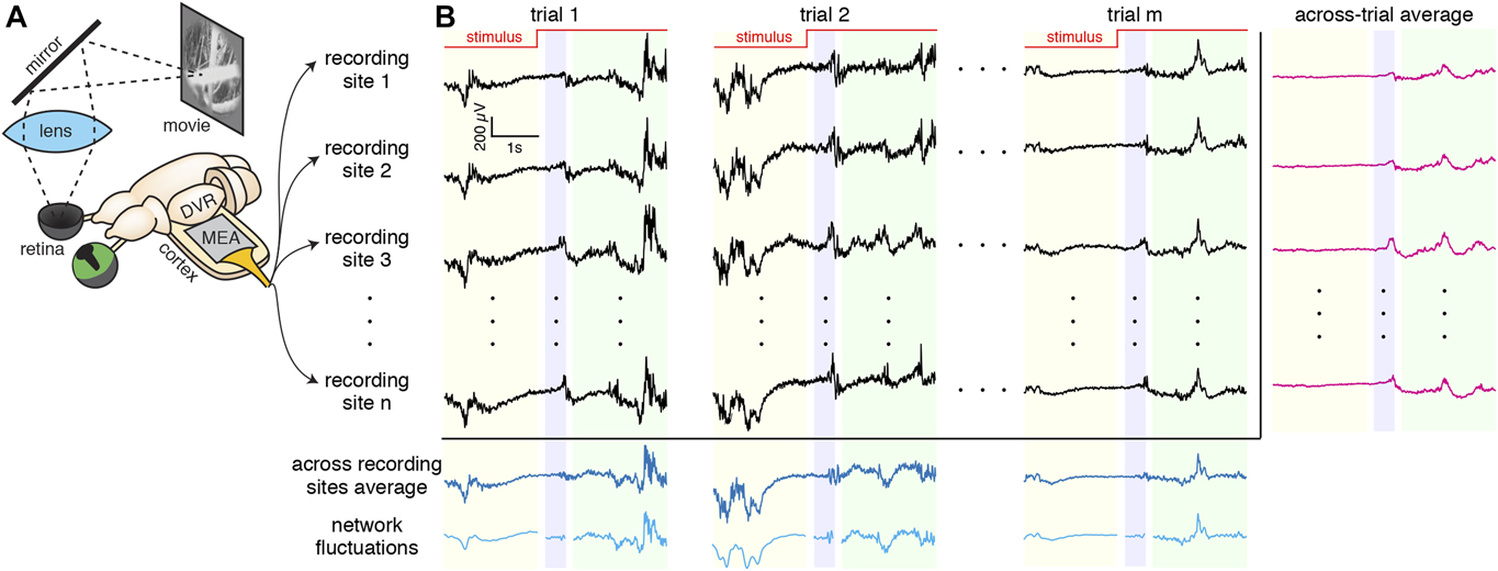
To investigate the dynamics and sources of cortical response variability and its correlations, we recorded and analyzed local field potentials (LFP) from visual cortex of turtle ex vivo preparations using microelectrode arrays (MEA) and decomposed cortical response variability into input, network, and local fluctuations (Fig. 1). Our results revealed that input fluctuations dominate cortical response variability immediately following stimulus onset, whereas network fluctuations dominate the response variability in the steady state during continued visual stimulation. Consistent with the dynamics of the relative contributions of input and network fluctuations to the response variability, we found that the network fluctuations dominate the correlations of the variability during the ongoing and steady-state epochs, but not immediately following stimulus onset. Finally, a parsimonious model of cortical circuit identified relevant network features mediating the dynamics and sources of cortical response variability and its correlations.
What are the relative contributions of input, network, and local fluctuations in visual responses in turtle cortex? (A) Our experimental setup for experiments done with a monitor and mirror. The visual stimuli are presented on a monitor. The image reflects off a mirror and through a lens to project on the retina of the turtle’s hemisected eye. LFP are recorded with a MEA placed in the flattened cortex. (B) LFP recordings (black) are shown for multiple trials and recording sites. Three epochs are being considered: ongoing (yellow), transient (blue), and steady state (green). The single-site across-trial average of the LFP recording (input fluctuation) is shown in magenta. The across recording sites average and “network fluctuation” are shown in dark and light blue, respectively.

Materials and methods
Ex vivo eye-attached whole-brain preparation
All procedures were approved by the Institutional Animal Care and Use Committees of both Washington University and University of Arkansas, and conform to the guidelines of the National Institutes of Health on the Care and Use of Laboratory Animals. As described in our previous work (Shew et al., Reference Shew, Clawson, Pobst, Karimipanah, Wright and Wessel2015), adult red-eared sliders (Trachemys scripta elegans, 150–1000 g weight, 12–15 cm carapace length) were studied. First, turtles were anesthetized with propofol (2 mg propofol/kg), then decapitated, and the brain was removed surgically from the skull, with eyes and optic nerve intact. The right eye was hemisected to expose the retina and bathed in cold extracellular saline (in mM, 85 NaCl, 2 KCl, 2 MgCl2·6H2O, 20 dextrose, 3 CaCl2–2H2O, 45 NaHCO3, bubbled with 95% O2 and 5% CO2). Two cuts were made to unfold the cortex, thus facilitating the subsequent insertion of the microelectrode array. Recordings began 2–3 h after induction of anesthesia.
Visual stimulation
Visual stimuli were delivered with either a video projector (Aaxa Technologies, P4X Pico Projector) or an LCD monitor (Samsung 19″, 1440 × 900 pixels, contrast ratio = 20,000:1, and response time = 2 ms) to the retina. Visual stimuli were as follows: a naturalistic movie (“CatCam”), a motion-enhanced movie (courtesy Jack Gallant), and a phase-shuffled version of the same movie. The duration of each movie was ∼10 s followed by 30 s of gray screen. A given visual stimulus was repeated between 15 and 20 times. The mean irradiance at the retina was 1 W/m2 for the projector and 20 mW/m2 for the monitor. In all cases, the stimulus was triggered using a custom Labview program (National Instruments).
Experimental design and statistical analysis
Extracellular neural activity recordings at multiple locations
Wideband (0.7 Hz–15 kHz) extracellular voltages were recorded at 30 kHz sample rate (Blackrock Microsystems, Cerebus) using two different electrode arrays. The first was a 96-channel MEA (10 × 10 square grid, 400 µm inter-electrode spacing, 500 µm electrode length, no corner electrodes, 50 kΩ impedance with Iridium oxide plating, Blackrock Microsystems). This array was inserted to a depth of 250–500 μm using a micromanipulator (Sutter, MP-285) with the plane of electrodes parallel to the dorsal surface of the cortex. The second array was a three-dimensional (3D) grid of electrodes (4 × 4 × 8 grid, 16 shanks, 8 electrodes per shank, 300 μm inter-shank spacing, 100 μm inter-electrode spacing on each shank, 300 kΩ impedance with Iridium oxide plating, Neuronexus) and was inserted to a depth such that electrodes spanned the cortex from the ventricular to the dorsal surface. To avoid LFP cross-talk, we analyzed data from only one electrode per shank that has the strongest response. With postprocessing filtering (bandpass), we extracted the local field potential (LFP)  $Y_j^k\left( t \right)$ at recording site j for trial k. All data analysis was performed using custom-written software in MATLAB.
Identifying responsive recording sites
To identify visually responsive recording sites and include them in the analyses, we quantified the level of spontaneous LFP activity on each recording site by averaging over a 4 s time window preceding the stimulus onset. Then, we took responses over a 4 s window immediately following the stimulus onset and we defined the normalized difference of these two quantities as a measure of responsiveness. We classified a recording site as visually responsive if the ratio was greater than 0.75. This approach yields ∼10 (range: 6 to 14) visually responsive sites across all recordings.
Identifying sources of response variability
To identify sources of response variability, we used LFPs rather than spikes since (1) spikes were not clearly measurable in our experiments, and (2) LFP may better represent a large population of neurons. Nevertheless, these findings may be generalizable to the spiking data since LFP and spiking activity are correlated (see Fig. S4 in Shew et al., Reference Shew, Clawson, Pobst, Karimipanah, Wright and Wessel2015). From the LFP recordings  $Y_j^k\left( t\right)$ at the recording site j for trial k, we computed a number of useful quantities. The single-site across-trial average of the LFP recording is
 ${\left\langle {Y_j^k\left( t\right)} \right\rangle _{{\rm{trials}}}}$, which may be interpreted as the “input fluctuation.” The residual LFP recording at the recording site j for trial k is
 $Y_j^k\left( t\right) - {\left\langle {Y_j^k\left( t\right)} \right\rangle _{{\rm{trials}}}}$. The across recording sites average of the LFP recording for trial k is
 ${\left\langle {Y_j^k\left( t\right)} \right\rangle _{{\rm{sites}}}}$. By applying a Gaussian-process factor analysis (GPFA) (Yu et al., Reference Yu, Cunningham, Santhanam, Ryu, Shenoy and Sahani2009) to the across recording sites average of LFP recordings 〈Y k(t)〉sites, we obtained a smooth version of the across recording sites average of the LFP recordings X k(t), which may be interpreted as the “network fluctuation.” Even though the GPFA has been developed for spike count data, because LFP and spiking activity are correlated (see Fig. S4 in Shew et al., Reference Shew, Clawson, Pobst, Karimipanah, Wright and Wessel2015), it can bridge between the network state and the LFP activity. Indeed, the network state obtained using GPFA is very similar to low-frequency LFPs taken as an estimation of the network state (Kelly et al., Reference Kelly, Smith, Kass and Lee2010). Armed with these quantities, we assume that the LFP recording
 $Y_j^k\left( t\right)$ at the recording site j for trial k consists of the sum of three components:
 $$Y_j^k\left( t\right) = {\left\langle {Y_j^k\left( t\right)} \right\rangle _{{\rm{trials}}}} + {C_j}{X^k}\left( t\right) + \eta _j^k\left( t\right),$$
where C j is the coefficient that determines the strength of impact of the smoothed network fluctuation on the LFP recording of the recording site j. Following previous studies (Yu et al., Reference Yu, Cunningham, Santhanam, Ryu, Shenoy and Sahani2009), the parameters of the GPFA model were fit using an expectation-maximization (EM) algorithm in such a way that it maximized the probability of the observed LFP recording,  $Y_j^k\left( t\right)$. Finally, the remainder of the LFP recording
 $Y_j^k\left( t\right)$ that is not accounted for by the “input fluctuation”
 ${\left\langle {Y_j^k\left( t\right)} \right\rangle _{{\rm{trials}}}}$ and the “network fluctuation” X k(t) is collected in the term
 $\eta _j^k\left( t\right)$, to which we refer as the “local fluctuation.”
The traditional “variance explained” (ψ) is computed as the difference of the total variance and the variance of the residuals of a model, that is, the difference between the single-trial time series and the trial-averaged time series. Applied to our LFP recordings, the “variability explained” (ψ input) by input fluctuation is given by (David & Gallant, Reference David and Gallant2005; Haefner & Cumming, Reference Haefner and Cumming2008): 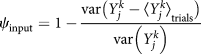 ${\psi _{{\rm{input}}}} = 1 - {{{\mathop{\rm var}} \left\big( {Y_j^k - {{\left\langle {Y_j^k} \right\rangle }_{{\rm{trials}}}}} \right\big)} \over {{\mathop{\rm var}} \left( {Y_j^k} \right)}}$. Expanding on this framework, the “variability explained” (ψ network) by the network fluctuation is defined by
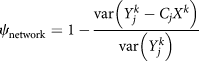 ${\psi _{{\rm{network}}}} = 1 - {{{\mathop{\rm var}} \left( {Y_j^k - {C_j}{X^k}} \right)} \over {{\mathop{\rm var}} \left( {Y_j^k} \right)}}$.
Defining three analysis windows
We considered three separate analysis windows relative to the timing of the stimulus onset: ongoing (2000 ms before stimulus onset), transient (200 to 600 ms after stimulus onset, but see below for details), and steady-state (800 to 2800 ms after stimulus onset). We motivated our choice of windows based on the results of a previous study of population activity performed on the same data set (Shew et al., Reference Shew, Clawson, Pobst, Karimipanah, Wright and Wessel2015). The choice of a relatively long transient time window and a 200 ms gap before it is because LFP responses are delayed by >200 ms past the stimulus onset (see Fig. S5 in Shew et al., Reference Shew, Clawson, Pobst, Karimipanah, Wright and Wessel2015; Wright et al., Reference Wright, Hoseini and Wessel2017a). This delay is likely mediated by the processing time from photoreceptors to the visual cortex in turtle. We repeated all of our analysis for three other sets of choices for epoch window sizes (three 1-s) and gaps between epochs (Wright et al., Reference Wright, Hoseini and Wessel2017a). The results presented here were largely robust to these choices (data not shown).
Correlated variability analysis
As mentioned above, for each single-trial LFP, the residual (or deviation from the trial averaged activity LFP recording) is calculated by subtracting the across-trial average time series from the single-trial time series, that is, the residual LFP recording at the recording site j for trial k is  $Y_j^k\left( t\right) - {\left\langle {Y_j^k\left( t\right)} \right\rangle _{{\rm{trials}}}}$. Traces were then separated into three epochs, as detailed above. Then Pearson correlation of residuals
 $Y_j^k\left( t\right) - {\left\langle {Y_j^k\left( t\right)} \right\rangle _{{\rm{trials}}}}$ between pairs of responsive recording sites was calculated for each epoch and trial k. The results were averaged across all trials, resulting in the trial-averaged correlated variability (CC) for each pair and epoch. The significance of CC values for a given pair and epoch was determined by either one-sided or two-sided t-test.
Assuming that the LFP recording  $Y_j^k\left( t\right)$ at recording site j for trial k consists of the sum of three components (see above), the local fluctuations were
 $\eta _j^k\left( t\right) = Y_j^k\left( t\right) - {\left\langle {Y_j^k\left( t\right)} \right\rangle _{{\rm{trials}}}} - {C_j}{X^k}\left( t\right)$. Within this analysis framework, we then calculated the Pearson correlation of the local fluctuations between pairs of responsive recording sites for each epoch and trial k.
Phase concentration analysis
For each trial and LFP recording site, we extracted a 5.8 s window of residuals and residuals with network fluctuation subtracted. To avoid filtering artifacts at the beginning and end of the signal, we padded it with two 500 ms traces and later on dropped it. For each trace, we performed wavelet analysis in Matlab using software provided by C. Torrence and G. Compo (Torrence and Compo, Reference Torrence and Compo1998) (available at URL: http://paos.colorado.edu/research/wavelets/). This resulted in a phase value as a function of time and frequency for trial k and recording site i,  $\varphi _i^k\left( {t,f} \right)$. We then calculated the cosine of the phase difference for pair ij,
 $R_{ij}^k\left( {t,f} \right) = \cos \left[ {\varphi _i^k\left( {t,f} \right) - \varphi _j^k\left( {t,f} \right)} \right]$, and averaged over the entire frequency range () and then time to obtain the “phase concentration” for each epoch and all the possible pairs, R ij(epoch). The phase concentration ranges between −1 and +1, with +1 for a pair of perfectly in-phase signals, −1 for perfectly out-of-phase signals, and 0 for two signals with random phase difference.
Computational model
We simulated a two-dimensional model network of 800 excitatory and 200 inhibitory leaky integrate-and-fire neurons using code written in Python. All neurons are distributed randomly on the surface of a unit sphere (in order to have periodic boundary condition). In the model that reproduced our principal experimental results, excitatory connections had clustered (or “small-world”) connectivity, that is, connections were made between nearby neurons with a probability that has 0.1 maximum and decay like a Gaussian with spatial separation of the neurons (Watts & Strogatz, Reference Watts and Strogatz1998; Litwin-Kumar & Doiron, Reference Litwin-Kumar and Doiron2012; Bujan et al., Reference Bujan, Aertsen and Kumar2015). All other connections were established randomly without any spatial constraint. This network topology has a mean path length and high clustering coefficient (Aguirre et al., Reference Aguirre, Huerta, Corbacho and Pascual2002). Synaptic weights are drawn from a gamma distribution with a very long tail (Cossell et al., Reference Cossell, Iacaruso, Muir, Houlton, Sader, Ko, Hofer and Mrsic-Flogel2015). The dynamics of the membrane potential (V i) of each neuron evolved according to
 $${\tau _{\rm{m}}}{{{\rm{d}}{V_i}} \over {{\rm{d}}t}} = - {g_{\rm{L}}}\left[ {{V_i}\left( t\right) - {E_{\rm{L}}}} \right] + {I_{{\rm{syn}}}}\left( t\right),$$
where the membrane time constant τ m = 100 ms (excitatory neurons), 50 ms (inhibitory), and the leak conductance g L = 10 nS (excitatory) and 5 nS (inhibitory). The leak reversal potential E L for each neuron was a random value between −70 and −60 mV, drawn from a Gaussian distribution. The reversal potentials for the synaptic current I syn(t) were E GABA = −68 mV and E AMPA = 50 mV. The spike threshold for each neuron was −40 mV. A neuron reset to −59 mV after spiking, and was refractory for 2 ms (excitatory) and 1 ms (inhibitory).
The synaptic current is given by  $I_{{\rm{syn}}}^{{\rm{YX}}}\left( t\right) = {g_{{\rm{YX}}}}{S_{{\rm{YX}}}}\left( t\right)\left( {V\left( t\right) - {E_{{\rm{syn}}}}} \right)$, where g YX is the maximum conductance and gating variable, S YX(t), following a presynaptic spike at time 0 is described by (Hoseini & Wessel, Reference Hoseini and Wessel2016)
 $${S_{{\rm{YX}}}}\left( t\right) = {{{\tau _{\rm{m}}}} \over {{\tau _{{\rm{DYX}}}} - {\tau _{{\rm{RYX}}}}}}\left[ {\exp \left( { - {{t - {\tau _{{\rm{LX}}}}} \over {{\tau _{{\rm{DYX}}}}}}} \right) - \exp \left( { - {{t - {\tau _{{\rm{LX}}}}} \over {{\tau _{{\rm{RYX}}}}}}} \right)} \right].$$
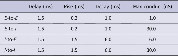
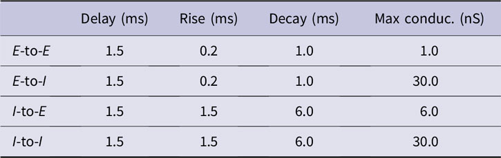
Each synapse type (between presynaptic neurons of type X and postsynaptic neurons of type Y) had three relevant time course parameters: delay (τ LX, i.e., the lag between presynaptic spike time and beginning of conductance waveform), rise time (τ RYX), and decay time (τ DYX). Values are listed in Table 1.
Parameters of the simulated model
In response to a presynaptic spike, the weight (W YX) of a synapse depressed and recovered according to
 $${{{\rm{d}}{W_{{\rm{YX}}}}\left( t\right)} \over {{\rm{d}}t}} = - {{{W_{{\rm{YX}}}}\left( t\right)} \over {{\tau _{{\rm{depress}}}}}}\delta \left( {t - t_{\rm{X}}^{{\rm{sp}}}} \right) + {{W_{{\rm{YX}}}^0 - {W_{{\rm{YX}}}}\left( t\right)} \over {{\tau _{{\rm{recover}}}}}},$$
where  $W_{{\rm{YX}}}^0$ is the initial weight matrix, depression time constant τ depress = 30 ms, and recovery time constant τ recover = 1.5 s.
Twenty external independent Poissonian inputs are fed into each neuron. During “ongoing” activity, the total external input was 180 Hz (20 inputs, 6 Hz each). The stimulus was modeled as a sudden increase to 800 Hz at stimulus onset time.
The gating variables for external inputs had the same parameters as for E-to-E connections, and maximum conductances were g E = 4 nS. Each trial was 5.8 s in duration, with the stimulus onset at 2.7 s, and the time step was 0.05 ms. The ongoing epoch was defined to be 2200 ms to 200 ms before stimulus onset, the transient epoch 0 ms to 400 ms after stimulus onset, and the steady-state epoch 600 ms to 2600 ms after stimulus onset. The additional half a second at the beginning and end of each trial ensured there were no wavelet filtering artifacts in the ongoing and steady-state epochs.
We imagined 10 equidistant electrodes on the surface of the sphere and defined simulated LFPs as the summation over synaptic currents to a population of excitatory neurons in the vicinity of the nearest electrode.
Code that was used to simulate the network is available on https://github.com/Mahmood-Hoseini/Cortical-response-variability-and-noise-correlation.
Results
To quantify response variability, its dynamics, and its correlation across visual cortex, we recorded population neural activity (local field potential, LFP)  $Y_j^k\left( t\right)$ for multiple trials k at multiple recording sites j using a microelectrode array (MEA) inserted into the geniculo-recipient dorsal cortex (visual cortex) of 11 turtle ex vivo eye-attached whole-brain preparations during visual stimulation of the retina (Fig. 1A). Turtle dorsal cortex consists of a single layer of densely packed somata of pyramidal neurons, sandwiched between layers filled with axons, dendrites, and a diverse population of interneurons (Swanson, Reference Swanson2003). We aimed to select recording sites in the vicinity of the single layer of pyramidal neuron somata. LFP responses to repeated presentations of extended stimuli varied from trial to trial, with a response variability magnitude as large as the trial-averaged response (Fig. 1B).
The contribution of input fluctuations to cortical response variability increases sharply during the transient epoch
How does the response variability vary with time relative to the visual stimulus onset? What sources contribute to the response variability? To address these questions, we considered three separate analysis windows (Fig. 1B): ongoing (2000 ms before stimulus onset), transient (200 to 600 ms after stimulus onset), and steady state (800 to 2800 ms after stimulus onset) (Methods). From the LFP recordings  $Y_j^k\left( t\right)$ at recording sites j for trials k, we inferred three sources of response variability. First, we interpreted the across-trial average of the LFP recording
 ${\left\langle {Y_j^k\left( t\right)} \right\rangle _{{\rm{trials}}}}$ as a measure of the “input fluctuation” at recording site j (Fig. 1B). Second, applying a Gaussian-process factor analysis (GPFA) (Yu et al., Reference Yu, Cunningham, Santhanam, Ryu, Shenoy and Sahani2009) to the across recording sites average of LFP recordings 〈Y k(t)〉sites, we obtained a measure of the “network fluctuation” X k(t) for trial k (Fig. 1B). Third, we assumed that the sources of response variability combine additively, that there are exactly three sources, and that the contribution of network fluctuations to the response variability is site specific (Methods). Within these assumptions, the LFP recording
 $Y_j^k\left( t\right)$ at the recording site j for trial k can be written as
 $Y_j^k\left( t\right) = {\left\langle {Y_j^k\left( t\right)} \right\rangle _{{\rm{trials}}}} + {C_j} \cdot {X^k}\left( t\right) + \eta _j^k\left( t\right)$, where C j is the coefficient that determines the strength of impact of the network fluctuation on the LFP recording of recording site j. The term
 $\eta _j^k\left( t\right)$ accounts for the “local fluctuation.” Armed with this analysis framework, we then calculated the LFP response variability explained in visual cortex during natural vision for the three sources of fluctuations in the three time windows relative to the stimulus onset.
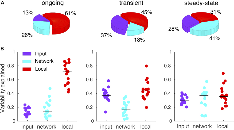
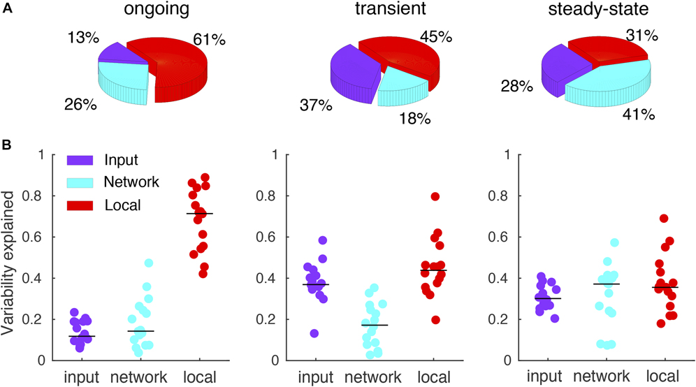
Compared with the ongoing and steady-state period, during the transient period, the contribution of input fluctuations to the response variability increased, whereas the contribution of network fluctuations decreased (ongoing: 13%, 26%, and 61% for input, network, and local fluctuations, respectively; transient: 37%, 18%, and 45%; steady state: 28%, 41%, and 31%) (Fig. 2A). These observations held for 8/11 turtles and 3 types of visual stimuli (n = 16 data sets; naturalistic movie and motion enhanced movies as well as its phase shuffled version; see Fig. 2B), demonstrating their generality. Furthermore, results were largely robust with respect to the choices of window sizes and gaps between windows (data now shown). In terms of cortical circuit architecture, the observed sharp increase of the input fluctuations during the transient epoch suggests that cortical response fluctuations following stimulus onset are largely driven by the activity fluctuations of the thalamic inputs to the cortex (Shadlen & Newsome, Reference Shadlen and Newsome1998; Salinas & Sejnowski, Reference Salinas and Sejnowski2000; de la Rocha et al., Reference de la Rocha, Doiron, Shea-Brown, Josić and Reyes2007; Renart et al., Reference Renart, de la Rocha, Bartho, Hollender, Parga, Reyes and Harris2010; Rosenbaum, Reference Rosenbaum2010).
The relative contribution of input fluctuations to the response variability increases during the transient epoch. (A) Pie charts show contribution of the three sources (input, network, and local fluctuations) in the variability of responses across three epochs (ongoing, transient, and steady state) for a single recording. (B) The contribution of three sources in response variability across the three epochs for 16 recording sessions of 11 preparations (Five preparations were recorded twice). The relative contribution of input fluctuations during the ongoing epoch is significantly lower than the other two epochs (ongoing, transient, steady state; mean ± SEM; 0.13 ± 0.01, 0.38 ± 0.02, 0.30 ± 0.01; F = 47, P = 7.8 × 10⁻¹², one-way ANOVA, Tukey’s post hoc test, n = 16; ongoing vs. transient, P = 9.6 × 10⁻¹¹; ongoing vs. steady state, P = 9.4 × 10⁻⁹; transient vs. steady state, P = 0.02). In contrast, the relative contribution of network fluctuations to the response variability increases significantly during the steady-state epoch (0.18 ± 0.03, 0.17 ± 0.03, 0.31 ± 0.04; F = 6, P = 0.003; ongoing vs. transient, P = 0.95; ongoing vs. steady state, P = 0.01; transient vs. steady state, P = 0.005). Local fluctuation has a higher contribution during the ongoing epoch (0.68 ± 0.04, 0.45 ± 0.04, 0.37 ± 0.03; F = 20, P = 7.2 × 10⁻⁷; ongoing vs. transient, P = 1 × 10⁻⁴; ongoing vs. steady state, P = 9 × 10⁻⁸; transient vs. steady state, P = 0.32).
Network fluctuations dominate the correlated variability during the ongoing and steady-state epochs
The interconnected nature of cortical circuits suggests that cortical response variability across trials is to some extent correlated among recorded signals (Cohen & Kohn, Reference Cohen and Kohn2011; Tan et al., Reference Tan, Chen, Scholl, Seidemann and Priebe2014; Scholvinck et al., Reference Scholvinck, Saleem, Benucci, Harris and Carandini2015). Given the observed dynamics of cortical response variability (Fig. 2), we asked to what extent the correlation of variability varies with time relative to the visual stimulus onset.
To obtain the “correlated variability,” or noise correlation, for a given trial k, we computed the Pearson correlation coefficient between pairs of LFP recordings (0.7–100 Hz) around the trial average from two recording sites j and i for trial k, that is, the Pearson correlation coefficient of the so-called residuals  $Y_j^k\left( t\right) - {\left\langle {Y_j^k\left( t\right)} \right\rangle _{{\rm{trials}}}}$ and
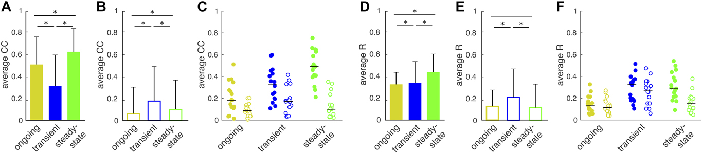
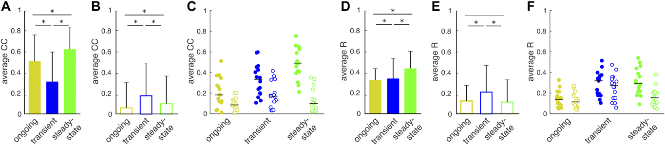
 $Y_i^k\left( t\right) - {\left\langle {Y_i^k\left( t\right)} \right\rangle _{{\rm{trials}}}}$. We averaged across all trials to compute the trial-averaged correlated variability CC for a given pair of recording sites j and i. Finally, averaging across all possible pairs of recording sites, we obtained the population-averaged correlated variability 〈CC〉. Correlated variabilities during ongoing, transient, and steady-state epochs were significantly nonzero for all epochs and dropped significantly during the transient epoch (mean ± SEM, 0.51 ± 0.01, 0.31 ± 0.03, 0.62 ± 0.02; F = 73, P = 1 × 10⁻²⁴, one-way ANOVA; Fig. 3A).
After subtraction of network fluctuations, correlated variability follows oscillation dynamics in the network. (A) Correlated variability of the residuals for a single recording significantly decreases from ongoing to transient and then recovers back during steady-state epoch. Bars indicate average over all the possible pairs (mean ± SEM, 0.51 ± 0.01, 0.31 ± 0.03, 0.62 ± 0.02; F = 73, P = 1 × 10⁻²⁴, one-way ANOVA, n = 66). (B) Correlated variability amplitudes for the data shown in A, markedly decrease during ongoing and steady state after subtracting network fluctuations (0.06 ± 0.02, 0.17 ± 0.03, 0.10 ± 0.03; F = 5, P = 0.005). (C) A transient increase in correlated variability emerges after subtracting of network activity. The dots represent the preparations (ongoing, transient, steady state; filled circles, residuals, 0.21 ± 0.04, 0.33 ± 0.04, 0.49 ± 0.04; F = 14, P = 1 × 10⁻⁵, one-way ANOVA, Tukey’s post hoc test, n = 16; ongoing to transient, P = 0.07; ongoing to steady state, P = 7 × 10⁻⁶; transient to steady-state, P = 0.009; open circles, residuals with network fluctuation subtracted, 0.09 ± 0.01, 0.18 ± 0.03, 0.12 ± 0.03; F = 3, P = 0.03; ongoing to transient, P = 0.04; ongoing to steady state, P = 0.63; transient to steady state, P = 0.27). (D) Phase concentration of the residuals for a single recording significantly increases from transient to steady state (0.32 ± 0.01, 0.34 ± 0.02, 0.44 ± 0.02; F = 18, P = 8 × 10⁻⁹). (E) Phase concentration increases from ongoing to transient and decreases from transient to steady-state epochs after subtracting network fluctuations (0.12 ± 0.01, 0.20 ± 0.02, 0.11 ± 0.02; F = 9, P = 0.001). (F) Subtraction of network activity highlights the transient increase in phase concentration. The dots represent the preparations (0.14 ± 0.02, 0.24 ± 0.03, 0.31 ± 0.03; F = 11, P = 1 × 10⁻⁴; ongoing to transient, P = 0.001; ongoing to steady state, P = 2 × 10⁻⁵; transient to steady state, P = 0.88; 0.12 ± 0.02, 0.26 ± 0.03, 0.16 ± 0.02; F = 8, P = 0.001; ongoing to transient, P = 0.001; ongoing to steady state, P = 0.56; transient to steady state, P = 0.02).
Within our assumption of three additive components of cortical response variability (see above), the residuals  $Y_j^k\left( t\right) - {\left\langle {Y_j^k\left( t\right)} \right\rangle _{{\rm{trials}}}}$ equal
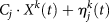 ${C_j} \cdot {X^k}\left( t\right) + \eta _j^k\left( t\right)$. This identity raises the question to what extent the two components, that is, network fluctuations C j · X k(t) and local fluctuations
 $\eta _j^k\left( t\right)$, contribute to the correlated variability. To address this question, we next computed the Pearson correlation coefficients of
 $Y_j^k\left( t\right) - {\left\langle {Y_j^k\left( t\right)} \right\rangle _{{\rm{trials}}}} - {C_j} \cdot {X^k}\left( t\right)$ and
 $Y_i^k\left( t\right) - {\left\langle {Y_i^k\left( t\right)} \right\rangle _{{\rm{trials}}}} - {C_i} \cdot {X^k}\left( t\right)$ from two recording sites j and i for trial k. The thus computed correlation coefficients were markedly reduced for the ongoing and steady-state epochs, but changed little for the transient epoch (0.06 ± 0.02, 0.17 ± 0.03, 0.10 ± 0.03; F = 5, P = 0.005; Fig. 3B). Similar results were obtained for all 16 data sets (Fig. 3C). In summary, there are three noticeable features comparing CC amplitudes before and after accounting for the network fluctuations. First, accounting for the network fluctuations reduces CC values for all epochs. Second, ongoing and steady-state CCs are more heavily influenced by network fluctuations due to the high fraction of variance captured by the GPFA model. Third, a transient increase in correlated variability emerges after subtracting network activity for all the preparations (Fig. 3A–3C, ongoing, transient, and steady state; 0.21 ± 0.04, 0.33 ± 0.04, 0.49 ± 0.04; F = 14, P = 1 × 10⁻⁵, one-way ANOVA, Tukey’s post hoc test; ongoing to transient, P = 0.07; ongoing to steady state, P = 7 × 10⁻⁶; transient to steady state, P = 0.009; open circles, residuals with network fluctuation subtracted, 0.09 ± 0.01, 0.18 ± 0.03, 0.12 ± 0.03; F = 3, P = 0.03; ongoing to transient, P = 0.04; ongoing to steady state, P = 0.63; transient to steady state, P = 0.27).
It has been hypothesized that the coordination between pairs of neurons might be shaped by the amount of phase synchrony as well as anatomical connectivity (Renart et al., Reference Renart, de la Rocha, Bartho, Hollender, Parga, Reyes and Harris2010; Scholvinck et al., Reference Scholvinck, Saleem, Benucci, Harris and Carandini2015; Haider et al., Reference Haider, Schulz, Häusser and Carandini2016). We therefore asked how well correlated variability dynamics could be explained by the network phase synchrony. Specifically, unlike amplitude correlation, measures of phase synchronization are time-resolved and are only sensitive to the phases, irrespective of the amplitudes of the two signals. For a pair of analog signals, a popular measure of phase synchrony is the “phase concentration,” which is defined as the cosine of the phase difference of analog signals (Quiroga et al., Reference Quiroga, Kraskov, Kreuz and Grassberger2002; Yang et al., Reference Yang, Shew, Roy and Plenz2012) (see Methods). We calculated the cosine of phase difference between a pair of residuals, that is,  $Y_j^k\left( t\right) - {\left\langle {Y_j^k\left( t\right)} \right\rangle _{{\rm{trials}}}}$, or residuals while accounting for the network fluctuations, that is,
 $Y_j^k\left( t\right) - {\left\langle {Y_j^k\left( t\right)} \right\rangle _{{\rm{trials}}}} - {C_j} \cdot {X^k}\left( t\right)$, across epochs. Then, we obtained trial-average phase concentration, R, by taking the average over all trials and window of interest. The phase concentration takes a value of +1 for a pair of perfectly in-phase signals, −1 for perfectly out-of-phase signals, and 0 for two signals with random phase difference.
Our results indicated that, like correlated variability (Fig. 3A), population-averaged phase concentration (〈R〉) for residuals  $Y_j^k\left( t\right) - {\left\langle {Y_j^k\left( t\right)} \right\rangle _{{\rm{trials}}}}$ from pairs of recording sites was significantly increased from transient to steady-state epochs (0.32 ± 0.01, 0.34 ± 0.02, 0.44 ± 0.02; F = 18, P = 8 × 10⁻⁹; Fig. 3D). Qualitatively similar results were obtained for all 16 data sets (data not shown). When accounting for network fluctuations, that is,
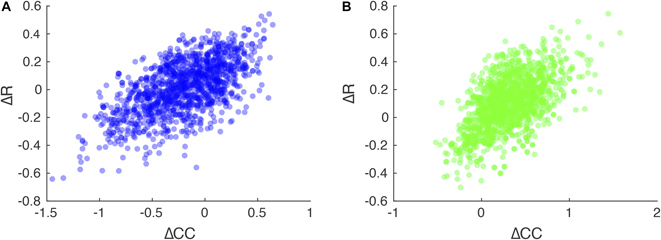
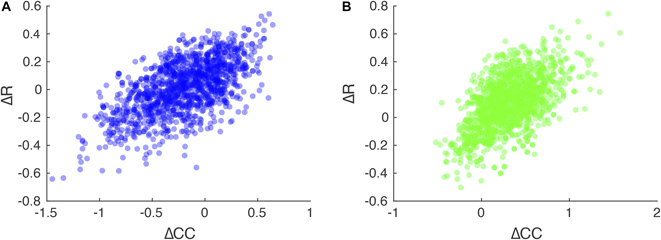
 $Y_j^k\left( t\right) - {\left\langle {Y_j^k\left( t\right)} \right\rangle _{{\rm{trials}}}} - {C_j} \cdot {X^k}\left( t\right)$, population-averaged phase concentration from pairs of recording sites were significantly reduced (0.12 ± 0.01, 0.20 ± 0.02, 0.11 ± 0.02; F = 9, P = 0.001; Fig. 3E). Furthermore, population-averaged phase concentration increased significantly from ongoing to transient and then decreased from transient to steady state, thus mirroring the dynamics of the correlation coefficients of network fluctuation corrected residuals (Fig. 3F). Indeed, changes in CC were significantly related to changes in R for residuals (Fig. 4A, from ongoing to transient epochs, ρ = 0.58; Spearman’s test, P ≪ 0.001; Fig. 4B, from transient to steady-state epochs, ρ = 0.54, P ≪ 0.001).
Changes in correlated variability are significantly correlated with changes in phase concentration. (A) Change in correlated variability from ongoing to transient epochs against changes in phase concentration from ongoing to transient reveals a significant correlation (Spearman’s ρ = 0.58, P ≪ 0.001, n = 1320). Each dot is from one pair of recordings averaged across trials. (B) Same as in A for changes from transient to steady-state epochs (ρ = 0.54, P ≪ 0.001).
In summary, similar temporal dynamics in correlated variability and phase concentration across all frequency bands up to 100 Hz (data not shown; Hoseini et al., Reference Hoseini, Pobst, Wright, Clawson, Shew and Wessel2017b) may indicate that cortical oscillations are instructing coordination of neuronal activity at the scale of LFPs (for review, see Ermentrout, Reference Ermentrout1996; Achuthan & Canavier, Reference Achuthan and Canavier2009; Wang, Reference Wang2010).
Synaptic clustering mediates the nature of response variability
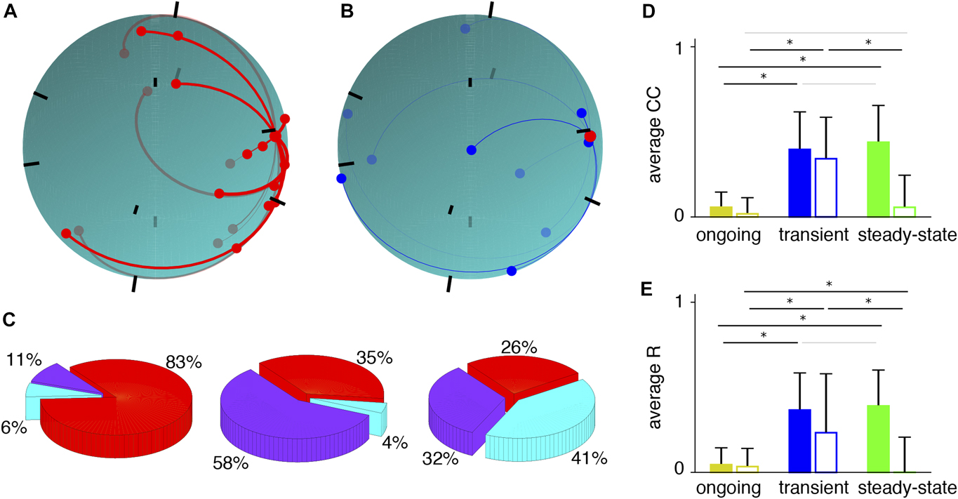
What biophysical mechanisms could mediate the experimentally observed response properties [i.e., nature of variability across epochs (Fig. 2)], and the dynamics of correlated variability and of phase concentration (Fig. 3)? To address this question, we investigated a model network of 800 excitatory and 200 inhibitory leaky integrate-and-fire neurons distributed randomly over the surface of a unit sphere, with Poisson process external inputs to all neurons (see Methods). In order to reproduce the experimental findings, we imposed a “small world” structure to the synaptic connectivity. Excitatory neurons make synapses to their neighbor excitatory cells with a Gaussian distribution decaying with spatial separation between neurons, with 10% connection probability (Fig. 5A). The rest of the connections are random, that is, I-to-E connections are homogeneously random such that an inhibitory neuron can project to any excitatory cell (Fig. 5B). Synaptic weights are drawn from a gamma distribution with a long tail (Cossell et al., Reference Cossell, Iacaruso, Muir, Houlton, Sader, Ko, Hofer and Mrsic-Flogel2015). An increase in the external input rate mimics the stimulus. Synaptic currents obey alpha function dynamics with reasonable sets of rise and decay times (Wang, Reference Wang1999; Brunel & Wang, Reference Brunel and Wang2003; Hoseini & Wessel, Reference Hoseini and Wessel2016), and we implemented adaptation via short-term synaptic depression with recovery (see Methods). We defined simulated LFPs as the summation over synaptic currents to a population of excitatory neurons. We simulated the network spiking in response to 20 repeated stimulus presentations. From the thus simulated LFPs, we computed the input  ${\left\langle {Y_j^k\left( t\right)} \right\rangle _{{\rm{trials}}}}$, network C j · X k(t), and local
 $\eta _j^k\left( t\right)$ fluctuations at each recording site and for all three epochs as described above.
A network with clustered architecture reproduces experimentally observed dynamics of variability and correlation. (A) E-to-E connections are clustered with sporadic long-range connections. Shown is the network projected onto the surface of a sphere. Excitatory synaptic connections to a given excitatory cell are shown with connection strength indicated in the thickness of the line. Black bars indicate the center of the calculated “LFP,” thus mimicking LFP recording electrodes. (B) Inhibitory inputs to the excitatory cell shown in A. I-to-E connections are homogeneously random such that an inhibitory neuron can project to any excitatory cell. (C) Portion of the variability explained by each component during the three epochs. (D) Average noise correlation across three epochs without (solid bars; ongoing, transient, steady state; 0.05 ± 0.01, 0.28 ± 0.03, 0.22 ± 0.04; F = 19, P = 5 × 10⁻⁸, n = 45; ongoing to transient, P = 7 × 10⁻⁸; ongoing to steady state, P = 4 × 10⁻⁵; transient to steady state, P = 0.24) and with (open bars; 0.03 ± 0.03, 0.24 ± 0.03, 0.03 ± 0.03; F = 41, P = 9 × 10⁻¹⁵; ongoing to transient, P = 9 × 10⁻¹⁰; ongoing to steady state, P = 0.99; transient to steady state, P = 7 × 10⁻¹⁰) subtraction of network fluctuations. Subtracting network fluctuations leads to a dramatic decrease in steady state correlation amplitudes. (E) Average noise correlation across three epochs without (solid bars; 0.03 ± 0.01, 0.36 ± 0.03, 0.39 ± 0.04; F = 22, P = 6 × 10⁻⁹; ongoing to transient, P = 7 × 10⁻⁷; ongoing to steady-state, P = 4 × 10⁻⁸; transient to steady-state, P = 0.43) and with (open bars; 0.02 ± 0.01, 0.23 ± 0.05, 0.00 ± 0.04; F = 22, P = 6 × 10⁻⁹; ongoing to transient, P = 3 × 10⁻¹¹; ongoing to steady state, P = 0.65; transient to steady state, P = 5 × 10⁻⁸) subtraction of network fluctuations.
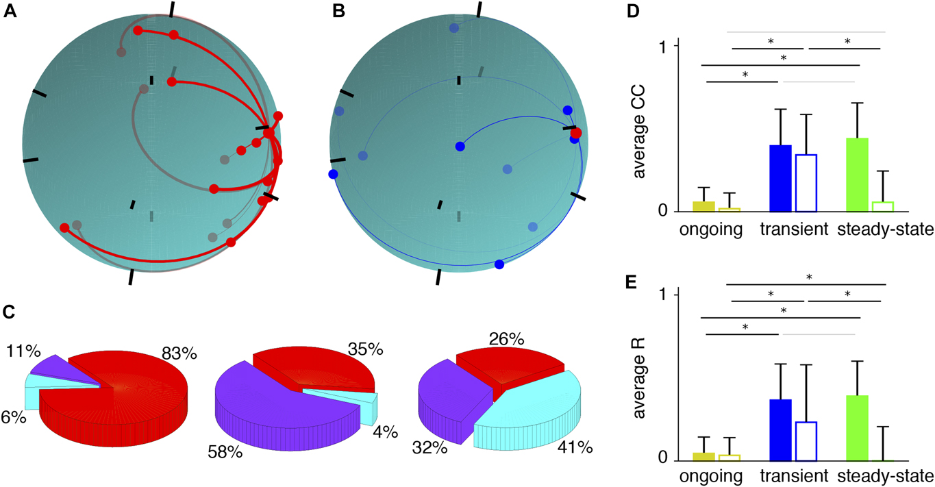
This model exhibits slow, coordinated spike-rate fluctuations (Litwin-Kumar & Doiron, Reference Litwin-Kumar and Doiron2012) with a reasonable propagation of activity from active clusters to more quiescent clusters (see Fig. 5 in Wright et al., Reference Wright, Hoseini and Wessel2017a). Comparing with the experimental results (Fig. 2), this model network reproduced qualitatively the fraction of variance explained by each component in the transient and steady-state epochs (Fig. 5C). Specifically, the simulated input fluctuations  ${\left\langle {Y_j^k\left( t\right)} \right\rangle _{{\rm{trials}}}}$ explain a large fraction of the total variability during the transient epoch, whereas the simulated network fluctuations X k(t) dominate during the steady state (ongoing: 11%, 6%, 83% for input fluctuations, network fluctuations, and local fluctuations, respectively; transient: 58%, 4%, and 35%; steady-state: 32%, 41%, and 26%). Correlated variabilities of simulated LFP residuals
 $Y_j^k\left( t\right) - {\left\langle {Y_j^k\left( t\right)} \right\rangle _{{\rm{trials}}}}$ during ongoing, transient, and steady-state epochs were significantly nonzero for all epochs (Fig. 5D), thus qualitatively reproducing the experimental results (Fig. 3A). Furthermore, when subtracting network fluctuations C j · X k(t) and computing the Pearson correlation coefficients of
 $Y_j^k\left( t\right) - {\left\langle {Y_j^k\left( t\right)} \right\rangle _{{\rm{trials}}}} - {C_j} \cdot {X^k}\left( t\right)$ and
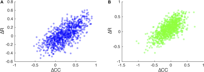
 $Y_i^k\left( t\right) - {\left\langle {Y_i^k\left( t\right)} \right\rangle _{{\rm{trials}}}} - {C_i} \cdot {X^k}\left( t\right)$ from two sites j and i for trial k, the thus computed correlation coefficients were markedly reduced for the ongoing and steady-state epochs, but changed little for the transient epoch (Fig. 5D). The transient increase of the thus computed correlation coefficients in model activity mirrors the experimentally observed dynamics (Fig. 3B). In addition, population-averaged phase concentration of residuals (Fig. 5E) roughly shows the same temporal dynamics as the simulated correlated variability (Fig. 3D). Indeed, changes in CC were significantly related to changes in R for both model (Fig. 6) and experiment (Fig. 4). Furthermore, accounting for the network fluctuations reduces 〈R〉 during the steady-state and causes 〈R〉 to show a significant increase with the stimulus onset (Fig. 5E), thus reproducing the observed dynamics of phase concentration (Fig. 3E).
Changes in correlated variability are significantly correlated with changes in phase concentration in the simulated network. (A) Change in correlated variability from ongoing to transient epochs against changes in phase concentration from ongoing to transient reveals a significant correlation (Spearman’s ρ = 0.58, P ≪ 0.001, n = 900). Each dot is from one pair of synthetic LFP signals averaged across trials. (B) Same as in A for changes from transient to steady-state epochs (ρ = 0.52, P ≪ 0.001).
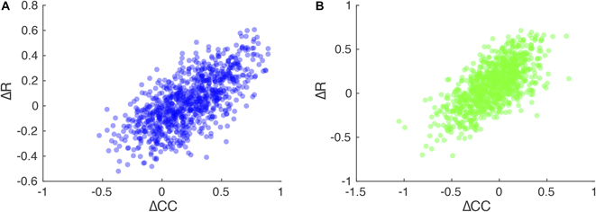
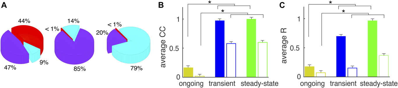
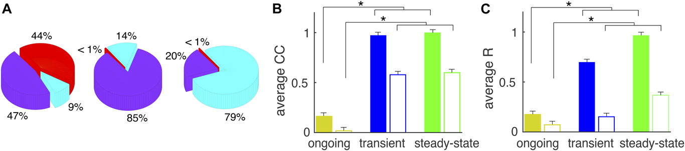
The following network features are essential in reproducing the observed network dynamics. First, the difference in time course of excitation and inhibition is important (Wright et al., Reference Wright, Hoseini and Wessel2017a). When synaptic time constants for excitation and inhibition are different, the lag between excitation and inhibition provides a window of opportunity in which synaptic input correlations are manifested in pairs of recordings (Renart et al., Reference Renart, de la Rocha, Bartho, Hollender, Parga, Reyes and Harris2010; Doiron et al., Reference Doiron, Litwin-Kumar, Rosenbaum, Ocker and Josić2016). This causes an increase in correlated variability as well as phase concentration (Fig. 5D and 5E), thus causing a tight relation between changes in correlated variability and changes in phase concentration (Fig. 6). Indeed, a network with equally fast excitation and inhibition does not exhibit any synchronization and fails to reproduce experimentally observed dynamics of 〈CC〉 as well as 〈R〉 (Wright et al., Reference Wright, Hoseini and Wessel2017a). Second, the synaptic depression is instrumental for the robustness of the results in a broad range of parameters such as initial synaptic weights, thalamic input rate, various time constants, and network architecture. Third, the synaptic depression and clustering structure are responsible for the significant 〈CC〉 decrease in correlated variability from transient to steady-state epoch. Synaptic depression diminishes network activity level by weakening interactions, which results in coherent oscillations occurring within one or a few clusters during steady-state epoch. Clustering architecture of the network, together with synaptic depression, abolishes oscillations in the network and causes a decrease in correlated variability 〈CC〉 values via the following mechanism. Stimulus onset triggers oscillations that invade the whole network. Such network oscillations at stimulus onset have two impacts. They cause an upward modulation in 〈CC〉 because oscillations are coherent and they cause the across-trial average to capture a large fraction of variability during the transient epoch since this network oscillation is consistent across trials. Consistent with this view, a homogenous random network reproduces the dynamics of response variability but not the dynamics of 〈CC〉 or 〈R〉 (Fig. 7). For completeness, we note that gamma distribution of the synaptic weights does not change any of the results except the amount of variability seen in 〈CC〉 and 〈R〉. In other words, a similar network with uniform distribution of weights, but still with clustered architecture, was able to reproduce the results.
A homogenous random network reproduces response variability results but not average CC or R. (A) Variability explained by each component during the three epochs shows absolute domination of input and network fluctuations during transient and steady-state epochs respectively. (B) Average CC (solid bars; ongoing, transient, steady-state; 0.16 ± 0.01, 0.97 ± 0.01, 0.99 ± 0.01; P ≪ 0.001, n = 900; open bars; 0.03 ± 0.01, 0.59 ± 0.01, 0.61 ± 0.01; P = 6.2 × 10⁻⁹). (C) Average phase concentration (solid bars; 0.17 ± 0.01, 0.69 ± 0.01, 0.96 ± 0.01, P ≪ 0.001; open bars; 0.06 ± 0.01, 0.14 ± 0.01, 0.32 ± 0.01, P = 4 × 10⁻⁴) indicates very large amplitudes during transient and steady-state epochs.
In conclusion, model investigations strengthen the hypothesis that thalamocortical oscillation are the key factor in reproducing experimental observations and, more importantly, clustering architecture shapes spatiotemporal dynamics of neural responses. Correlated variability follows network oscillation dynamics, such that constraining network model to produce realistic temporal dynamics of oscillations yields the transient increase in 〈CC〉. Therefore, synaptic time constants, synaptic clustering, and synaptic depression are intrinsic biophysical features relevant in reproducing experimental data.
Discussion
In this study, we measured cortical response variability and its correlation in visual cortex in order to answer three key questions: What are the sources of response variability? How do the relative contributions of the sources change following visual stimulus onset? What’s the plausible mechanism for observed temporal dynamics in variability? We found that input fluctuations dominate cortical response variability immediately following stimulus onset, whereas network fluctuations dominate the response variability in the steady state during continued visual stimulation. We also found that the network fluctuations dominate the correlations of the variability during the ongoing and steady-state epochs, but not immediately following stimulus onset. Through model simulations, we showed that synaptic time constants leading to oscillatory activity, and synaptic clustering and synaptic depression leading to spatially constrained pockets of coherent activity, can mediate the observed dynamics and sources of response variability and its coordination in visual cortex. Thus, our work sheds light on the yin and yang of externally generated (input fluctuations) and intrinsically generated (network fluctuations) variability of stimulus-modulated cortical activity and provides a link to realistic biophysical mechanisms and structural features in visual cortex.
Limitations of this study
First, in general, neuronal variability arises from sources internal and external to the brain. The external sources include environmental variables that impact neural activity (Renart & Machens, Reference Renart and Machens2014), sensory-motor coupling (Macrides & Chorover, Reference Macrides and Chorover1972; Shusterman et al., Reference Shusterman, Smear, Koulakov and Rinberg2011), animal locomotion (Chiappe et al., Reference Chiappe, Seelig, Reiser and Jayaraman2010; Niell & Stryker, Reference Niell and Stryker2010), and, specific to vision, eye movements (Findlay & Gilchrist, Reference Findlay and Gilchrist2003; Land & Tatler, Reference Land and Tatler2009), to name a few. To focus on brain-intrinsic sources of neuronal response variability, we chose the ex vivo whole-brain preparation for our studies (Llinás et al., Reference Llinás, Yarom and Sugimori1981). The choice of an ex vivo experimental approach, however, narrows the possibilities of suitable species, of which the turtle provides a robust ex vivo eye-attached whole-brain preparation (Hounsgaard & Nicholson, Reference Hounsgaard and Nicholson1990). Thus, the conclusions based on the experimental results are strictly limited to the turtle. It will be interesting to see to what extent these conclusions will generalize to other species, including humans.
Second, for the sake of experimental practicality and stable monitoring of cortical population activity, we chose to employ LFP recordings using a microelectrode array inserted into the geniculo-recipient dorsal cortex (visual cortex) of the turtle eye-attached whole-brain ex vivo preparation (Shew et al., Reference Shew, Clawson, Pobst, Karimipanah, Wright and Wessel2015; Clawson et al., Reference Clawson, Wright, Wessel and Shew2017; Hoseini et al., 2017Reference Hoseini, Pobst, Wright, Clawson, Shew and Wessela,Reference Hoseini, Pobst, Wright, Clawson, Shew and Wesselb). Both synaptic currents and spikes from many neurons within a volume around the recording electrode contribute to the LFP signal (Lindén et al., Reference Lindén, Tetzlaff, Potjans, Pettersen, Grün, Diesmann and Einevoll2011; Buzsáki et al., Reference Buzsáki, Anastassiou and Koch2012). Thus, conclusions on the sources of cortical variability from this study are strictly limited to the low-pass filtered, integrated synaptic and spiking activity represented in the recorded LFP signal. LFP recordings are thought to offer insights into the function and dynamics of neural circuits (Einevoll et al., Reference Einevoll, Kayser, Logothetis and Panzeri2013; Reimann et al., Reference Reimann, Anastassiou, Perin, Hill, Markram and Koch2013; Agarwal et al., Reference Agarwal, Stevenson, Berényi, Mizuseki, Buzsáki and Sommer2014; Senzai et al., Reference Senzai, Fernandez-Ruiz and Buzsáki2019). Nevertheless, future experiments should determine which aspects of our conclusions on cortical variability extend to neuronal spiking activity (Karimipanah et al., Reference Karimipanah, Ma, Miller, Yuste and Wessel2017) and membrane potential fluctuations (Wright and Wessel, Reference Wright and Wessel2017; Wright et al., 2017Reference Wright, Hoseini and Wessela,Reference Wright, Hoseini, Yasar and Wesselb) from identified cortical neurons in the context of simultaneously recorded network fluctuations.
Third, we considered exactly three additive sources of neural variability, that is, input, network, and local fluctuations. Given the exclusion of brain-external sources in the ex vivo brain preparation, this limitation seems justified. Nevertheless, the visual cortex (“local” and “network” fluctuations) receives projections not only from thalamus (“input” fluctuation) but also from other brain areas, for example, the dorsal ventricular ridge (Balaban, Reference Balaban1978; Desan, Reference Desan1984; Ulinski, Reference Ulinski1990). In our study, spatially homogeneous projections from other brain areas are largely absorbed in the “network” fluctuations category, whereas spatially inhomogeneous projections are partially absorbed in the “local” fluctuations category. Nevertheless, extending the monitoring of neural activity to ever larger volumes of the brain (Ji et al., Reference Ji, Freeman and Smith2016; Kim et al., Reference Kim, Zhang, Lecoq, Jung, Li, Zeng, Niell and Schnitzer2016) in future work will permit the inclusion of additional brain-intrinsic sources of neural variability.
Another potential caveat is that we only considered relative contribution of each source in response variability. An alternative approach would be to measure the strength of each component. Although these measurements may give us more insight into the dynamics of the network, they are sensitive to the signal-to-noise ratio of the traces and, hence, to the impedance of the recording sites (Kappenman & Luck, Reference Kappenman and Luck2010). Since we did not measure the impedance of the recording sites, we cannot estimate the absolute contributions.
The relative contributions of input and network fluctuations to cortical response variability evolve dynamically following stimulus onset
An important contribution of this study is the simultaneous evaluation of three brain-intrinsic sources of neuronal response variability at a given location in cerebral cortex. Input fluctuations can arise from variable responses in the lateral geniculate nucleus (Priebe & Ferster, Reference Priebe and Ferster2012; Sadagopan & Ferster, Reference Sadagopan and Ferster2012). Network fluctuations, including qualitatively different dynamics (Curto et al., Reference Curto, Sakata, Marguet, Itskov and Harris2009; Harris & Thiele, Reference Harris and Thiele2011), can arise from fluctuations across spatially extended scales of cortical circuit (Kelly et al., Reference Kelly, Smith, Kass and Lee2010; Ecker et al., Reference Ecker, Berens, James Cotton, Subramaniyan, Denfield, Cadwell, Smirnakis, Bethge and Tolias2014). Local fluctuations can arise from transmission noise in synapses and channel noise in membranes (Shadlen & Newsome, Reference Shadlen and Newsome1998; Carandini, Reference Carandini2004; Faisal et al., Reference Faisal, Aldo Faisal, Selen and Wolpert2008).
A number of experimental and computational techniques have attempted to shed light on the contributions of the three sources. For instance, cortical membrane potential variability remained nearly unaffected when inactivating the surrounding cortex, thus identifying the LGN input fluctuations as a dominant source of cortical response variability (Sadagopan & Ferster, Reference Sadagopan and Ferster2012). In contrast, response variability increased from LGN to visual cortex, and much of the added variability was accounted for by near-by cortical activity (Scholvinck et al., Reference Scholvinck, Saleem, Benucci, Harris and Carandini2015). More specifically, fluctuations in ongoing and stimulus-evoked population activity in visual cortex modulated cortical neuron responses to visual stimuli (Arandia-Romero et al., Reference Arandia-Romero, Tanabe, Drugowitsch, Kohn and Moreno-Bote2016) and spatial correlations in visual stimuli modulate cortical response variability (Rikhye & Sur, Reference Rikhye and Sur2015). Along those lines, when optogenetically silencing network fluctuations, isolated thalamic inputs to cortical neurons exhibited lower variability (Cohen-Kashi Malina et al., Reference Cohen-Kashi Malina, Malina, Mohar, Rappaport and Lampl2016). Furthermore, a model with stimulus-modulated rates and other-influences–mediated gain revealed that variability can originate in large part from local excitability fluctuations (Goris et al., Reference Goris, Movshon and Simoncelli2014). Another simple model that comprised two sources of shared variability, a uniform multiplicative gain and a neuron-specific additive offset, captured the variability of recorded spike counts in visual cortex (Lin et al., Reference Lin, Okun, Carandini and Harris2015).
In the context of these important earlier studies, the presented work advances our understanding of the origin and dynamics of cortical variability. We identify a dynamic that has not been shown in these earlier works, and we identify intrinsic cortical mechanisms that contribute to cortical response variability. Consistent with the previous work (Lin et al., Reference Lin, Okun, Carandini and Harris2015; Scholvinck et al., Reference Scholvinck, Saleem, Benucci, Harris and Carandini2015; Arandia-Romero et al., Reference Arandia-Romero, Tanabe, Drugowitsch, Kohn and Moreno-Bote2016), we assumed the existence of low-dimensional network fluctuation. We estimated the global fluctuation with Gaussian-process factor analysis (GPFA) (Yu et al., Reference Yu, Cunningham, Santhanam, Ryu, Shenoy and Sahani2009). Within this assumption, we quantified simultaneously the relative contributions and the dynamics of three sources, input, network, and local fluctuations, to the across-trial response variability in a visual cortex that is processing complex visual stimuli (Fig. 2).
The relative contribution of the three sources in response variability and the correlation amplitude across the three epochs are consistent with a cortical network adapting from a “disinhibited” to a “balanced” state. First, we found that both the average CC and relative contribution of input fluctuations to the response variability increase from ongoing to transient epochs. During this epoch, network is largely driven by the thalamocortical inputs which have shown to have low variability (Cohen-Kashi Malina et al., Reference Cohen-Kashi Malina, Malina, Mohar, Rappaport and Lampl2016) and high correlation (Bujan et al., Reference Bujan, Aertsen and Kumar2015). This state is well suited for robust driving of downstream cortical targets and beneficial for stimulus detection (Ollerenshaw et al., Reference Ollerenshaw, Zheng, Millard, Wang and Stanley2014). Second, while the relative contribution of network fluctuations to the response variability increases from transient to steady-state epochs, contribution of input fluctuations as well as average CC slightly decline. Adaptation in thalamic projections to the cortex may cause the decline in relative contribution of input fluctuations to the response variability during the steady-state epoch (Wang, Reference Wang2010; Ollerenshaw et al., Reference Ollerenshaw, Zheng, Millard, Wang and Stanley2014), leading to a more prominent role of intracortical connections with higher variability and lower average CC (Wright et al., Reference Wright, Hoseini and Wessel2017a). Together, during the steady-state epoch, network dynamic is largely determined internally (Scholvinck et al., Reference Scholvinck, Saleem, Benucci, Harris and Carandini2015; Cohen-Kashi Malina et al., Reference Cohen-Kashi Malina, Malina, Mohar, Rappaport and Lampl2016) to promote response fidelity (Zohary et al., Reference Zohary, Shadlen and Newsome1994) and stimulus discrimination (Gutnisky & Dragoi, Reference Gutnisky and Dragoi2008; Ollerenshaw et al., Reference Ollerenshaw, Zheng, Millard, Wang and Stanley2014). As such, these findings suggest that during visual processing, adaptation mechanisms mediate a transition between cortical coding schemes.
In future work, it will be promising to combine intervening experimental techniques like optogenetics with analytic tools like GPFA to investigate the biophysical mechanism and their dynamics of each variability component. Moreover, it would be interesting to use decoding methods (Dayan & Abbott, Reference Dayan and Abbott2003; Quiroga & Panzeri, Reference Quiroga and Panzeri2009) to extract information from each variability component. Previous works focus on how input fluctuation (trial-averaged activity) encodes stimulus information (Foffani & Moxon, Reference Foffani and Moxon2004; Cunningham & Yu, Reference Cunningham and Yu2014). However, what information of stimulus contained by low dimensional network fluctuation remains elusive and worth to be investigated in future.
From biophysical components to emergent oscillations and correlated variability
What combination of biophysical ingredients of a model network can generate the experimentally observed features? A variety of models have attempted to address the many facets of response variability and its correlation (Balaguer-Ballester, Reference Balaguer-Ballester2017). Nevertheless, despite many advances, the mapping from biophysical components to emergent response variability has proven challenging. Here, we addressed this question by developing a network of leaky integrate-and-fire neurons. The investigation revealed that time course of the synaptic currents, synaptic depression and recovery, and network architecture are the relevant underlying variables. Reasonable synaptic time constants cause ensemble oscillations to appear through the interaction of excitatory and inhibitory neurons (Wang, Reference Wang1999; Brunel & Wang, Reference Brunel and Wang2003). Stimulus onset triggers coherent oscillations and this correlates with the observed dynamics in both noise correlation (Fig. 3D and 3E) and phase concentration (Fig. 3H and 3I). Synaptic depression reduces activity level as well as interaction strength between the neurons. Therefore, later in time, spatially confined surge of activity happens within one or a few of the clusters (Wright et al., 2017Reference Wright, Hoseini and Wessela,Reference Wright, Hoseini, Yasar and Wesselb). As a result, noise correlation decreases as well as phase concentration. In addition, clustering architecture of the network provides a substrate for the neurons to influence their targets within the same cluster even after the operation of synaptic depression. Having less clustered connections leads to more global oscillations during ongoing and steady-state epochs, which alters the temporal dynamics of noise correlation and phase concentration.
In experiment, we observed the similar variability dynamic change across different types of stimuli, including naturalistic movie and artificial movie. The implication for understanding cortical networks is that dynamics in variability is largely determined internally. Consistently, our model shows that properties of synaptic connections are the keys to reproducing observed dynamics in variability.
Recent modeling work in the literature showed that recurrent circuit structure plays an important role in shaping neural variability (Van Vreeswijk & Sompolinsky, Reference Van Vreeswijk and Sompolinsky1996; Rosenbaum et al., Reference Rosenbaum, Smith, Kohn, Rubin and Doiron2017). For instance, spatially clustered connectivity is proposed to explain variability quenching after stimulus onset (Deco & Hugues 2012; Litwin-Kumar & Doiron, Reference Litwin-Kumar and Doiron2012) and the emergence of low-dimensional network fluctuation (Huang et al., 2019). Our work shows that, in addition to clustered connectivity, synaptic depression is also crucial for generating the transient variability dynamics we identified in the experiment.
Conclusion
In conclusion, we have provided key advances on two fronts, the dynamic sources and the mechanistic explanations of cortical response variability and their correlations. Together, our work showed the adaptation of different components in variability and correlated variability after stimulus onset. We provided an analytic method to track contributions of global fluctuations on cortical responses. Here, we analyzed data from ex vivo turtle brain. It could be meaningful to repeat the same analysis on behaving animals and study the relation between global fluctuation and behavior states. Moreover, it is reasonable to ask whether accounting for the shared component can either improve or impair discriminability of stimuli. Future experiments can be designed to address this question, whereas, for the simulated network, a linear decoder seems suitable (Moreno-Bote et al., Reference Moreno-Bote, Beck, Kanitscheider, Pitkow, Latham and Pouget2014) to quantify the change in information due to amplitude change in noise correlation by accounting for the shared fluctuations. Variability in visual responses comes from different sources, and a large portion of it does not depend on visual stimuli. By looking at different components of variability separately, we might be more likely to reach consistent conclusions from different dataset. Our results indicated that different components of variability dominate at different time and highlighted the contribution of global fluctuation on pairwise correlation between neuronal populations.
Supplementary material
Supplemental materials can be viewed in this issue of VNS by visiting https://doi.org/10.1017/S0952523819000117.
Acknowledgments
This research was supported by a Whitehall Foundation grant (#20121221; R.W.) and a NSF CRCNS grant (#1308159; R.W.).