1. The Problem of Variable Definition

Some choices of variables may lead to less informative, or even false, causal claims (Spirtes and Scheines Reference Spirtes and Scheines2004; Eberhardt Reference Eberhardt2016; Woodward Reference Woodward2016). Here is a classic example by Spirtes and Scheines (Reference Spirtes and Scheines2004). Consider the following hypothetical data-generating process (fig. 1). Total cholesterol (TC) is a deterministic function (e.g., the sum) of two variables, that is, low-density lipoproteins (LDL) and high-density lipoproteins (HDL), respectively known as “bad” and “good” cholesterol. The two cholesterols, in fact, have different causal roles: LDL causes heart disease (HD), while HDL prevents it. Moreover, assume that HDL and LDL cause, respectively, a disease called “disease 1” (D1) and a disease called “disease 2” (D2). Spirtes and Scheines point out that, if only TC but neither HDL nor LDL is observed, a manipulation of TC with respect to HD is “ambiguous” because it leaves underdetermined the values of TC’s underlying determinants, such that the effect on HD is unpredictable.

Figure 1.

Structure where the manipulation on TC with respect to HD is ambiguous.

In applied causal inference, often the variables under study are, like TC, functions of other variables with heterogeneous causal roles. For example, macroeconomics deals with aggregate variables such as gross domestic product, foreign sales, total imports, and so on, that are sums or averages of other variables, whose individual causal roles may be multifarious and opaque to the researcher. Often, the researcher cannot observe the underlying microbehaviors simply because statistical agencies provide aggregate data but do not reveal information on the single units. In other cases, collecting microdata may be too complex or costly. Treating aggregate variables as if they had a homogeneous causal role, however, may lead to less informative or false causal claims, as shown by the TC example. We will refer to an aggregate variable incurring such problems as ill-defined. Notice, thus, that whether a variable is ill-defined is relative to a variable set. That is, it may be ill-defined in one set but well-defined in another.

The problem of variable definition is often underestimated by the wider public. For instance, insufficient attention has been paid to its consequences for causal inference by constraint-based discovery methods (Spirtes, Glymour, and Scheines Reference Spirtes, Glymour and Scheines2000; Pearl Reference Pearl2009). We will return to this point in the next section, by showing how the presence of TC in a variable set may lead to wrong causal inferences. To address the problem, we introduce a representation framework—the “independent component” representation—for modeling structures containing two kinds of dependencies, namely, traditional causal dependencies between well-defined variables and dependencies between ill-defined variables and their determinants (see fig. 1). Finally, we demonstrate the potential of this framework for identifying ill-defined variables and reducing the risk of mistaken causal inferences.

2. Causal Search with Ill-Defined Variables

The last decades have witnessed the development and popularization of constraint-based causal discovery methods (Spirtes et al. Reference Spirtes, Glymour and Scheines2000; Pearl Reference Pearl2009). In this framework, a causal structure is represented as a triple 〈V, ℰ, Pr〉, where 〈V, ℰ〉 is a directed acyclic graph (DAG) consisting of a set V of variables and a set ℰ of edges among them, and Pr is the probability distribution over V associated to the DAG. The probability distribution Pr is assumed to comply with the Causal Markov Condition (CMC) and, typically, the Causal Faithfulness Condition (CFC). CMC says that

Here Par_i denotes the set of parents (direct causes) of V_i, and Non_i denotes the set of nondescendants (noneffects) of V_i. In other words, each variable is probabilistically independent of its noneffects, conditional on its direct causes. CMC presupposes that for every pair of variables in V, every common direct cause of the pair is in V or has the same value for all units in the population (causal sufficiency). CFC says:

CFC ensures that there is no causal dependence without probabilistic dependence; that is, all probabilistic independencies in the DAG correspond to causal independencies.

Based on these assumptions, constraint-based discovery methods are designed to recover the causal structure from data, by identifying conditional independencies among variables and then causally connecting variables not found to be independent. We now consider examples of simple data-generating processes including one ill-defined variable, TC, and show how using constraint-based methods based on conditional independencies—while ignoring that TC is ill-defined—may lead to mistakes. To anticipate, such mistakes involve apparent violations of CMC or CFC, which the search methods presuppose. Notice, however, that our interest here is not in providing novel counterexamples to CMC and CFC. These violations, in fact, could be avoided by choosing a “more suitable” variable set for causal inference—in this case, one featuring HDL and LDL instead of TC. And indeed, a formulation of CMC requiring that variables be independent of their noneffects conditional on their well-defined direct causes would not incur any violation. Here, however, we do not want to presuppose what counts as an ill-defined variable or a suitable variable set. Our goal is to avoid mistaken causal inferences in virtue of detecting ill-defined variables.

Suppose that, in $V=\{X,Y,Z\}$ , Y is the nondeterministic cause of both X and Z; that is, the true structure is $X\leftarrow Y\to Z$ . If all variables are well-defined, one can infer some properties of the causal structure by testing conditional independencies and applying a constraint-based discovery method. In particular, the independence $X⫫Z|Y$ and CFC allow one to exclude $X\to Y\leftarrow Z$ from the set of possible structures. Now, let the set of observed variables be $V^{\prime }=\{\mathrm{TC},D1,D2\}$ . That is, suppose again that one does not observe LDL and HDL but only TC. In this case, too, the true structure is not a collider. Assuming that the dependencies over V′ are causally interpretable, the most plausible structure—the one we wish to rationalize in this article—would be a common cause (i.e., $D1\leftarrow \mathrm{TC}\to D2$ ). However, since HDL and LDL are independent, $\mathrm{LDL}⫫\mathrm{HDL}$ , it follows that D1 and D2 are independent, too (i.e., $D1⫫D2$ ). If the true structure is a common cause, this contradicts CFC, which would entail a dependence between the effects of the common cause. Moreover, because D1 and D2 are dependent on (respectively) LDL and HDL, D1 and D2 become dependent upon conditioning on TC (i.e., $D1\overline{)⫫}D2|\mathrm{TC}$ ). For example, suppose one knows that one patient’s total cholesterol has increased. Then, knowing that disease 1 is absent gives one relevant information to predict that disease 2 is present. If the true structure is a common cause, this conditional dependence would violate CMC, which would entail the independence of D1 and D2 given their common cause. Based on $D1⫫D2$ and $D1\overline{)⫫}D2|\mathrm{TC}$ , as well as $\mathrm{TC}\overline{)⫫}D1$ and $\mathrm{TC}\overline{)⫫}D2$ , a constraint-based algorithm (e.g., the algorithms proposed by Spirtes et al. Reference Spirtes, Glymour and Scheines2000, 84–85, 144–45) will infer an unshielded collider on TC (i.e., $D1\to \mathrm{TC}\leftarrow D2$ ). A researcher applying the algorithm without knowing that TC is the sum of HDL and LDL (which are causes of, respectively, D1 and D2) will thus infer the wrong structure. The reason, ultimately, is that TC is ill-defined in V′.

Similarly, assume that all variables in V are well-defined, but now X causes Y, and Y causes Z; that is, the true structure is $X\to Y\to Z$ . Under CMC, it holds that $Z⫫X|Y$ , and under CFC, it holds that $X\overline{)⫫}Z$ . Now, consider the set of observed variables $V^{″}=\{\mathrm{Da},\mathrm{TC},D1\}$ , where Da (not represented in fig. 1), denoting dairies, is a cause of LDL but not of HDL. Again, suppose that one observes TC but neither HDL nor LDL. Here, too, the true structure is not a collider. The most plausible causal interpretation of the dependencies over V″ is a directed path (i.e., $\mathrm{Da}\to \mathrm{TC}\to D1$ ). However, since Da is a cause of LDL, which is independent of the cause HDL of D1, it holds that $\mathrm{Da}⫫D1$ , which violates CFC. Moreover, it holds that $\mathrm{Da}\overline{)⫫}D1|\mathrm{TC}$ , which violates CMC. From this, one may again wrongly infer a collider on TC (i.e., $\mathrm{Da}\to \mathrm{TC}\leftarrow D1$ ). Ultimately, the reason is that TC is ill-defined in V″.

These simple examples show how conditional independencies are sensitive to the presence of ill-defined variables in fork and chain structures, but ill-defined variables are undetectable from conditional independencies only.Footnote ¹ This may lead to mistaken inferences (i.e., the inference of colliders) if one unreflectively applies constraint-based algorithms.

3. A Novel Representation Framework

We now introduce a series of definitions, which will allow us to precisely define the notion of an ill-defined variable. First, we introduce a class of data-generating mechanisms inducing the problem of ill-defined variables. We call them “augmented” structural causal models, by which we extend the traditional notion of structural causal models (Pearl Reference Pearl2009; Peters, Janzing, and Schölkopf Reference Peters, Janzing and Schölkopf2017) to structures including deterministic assignments.

Model ℭ is defined over a set of variables $V=W\cup I$ with cardinality $n=m+k$ . We associate to ℭ a graph 𝒢_V (see, e.g., fig. 1, where TC is the only variable with a deterministic assignment). The graph 𝒢_V is obtained by creating a node for each element of V and by drawing a directed edge → from each parent in Par_i (if not empty) to W_i and a modified directed edge ⇒ from each determinant in Det_i to I_i. Henceforth, we restrict our attention to acyclic structures such that 𝒢_V is a modified DAG, to cases where Det_i has at least two elements, and to assignments A _W in which the shocks are additive. For simplicity, we also assume that no pair of variables I_i, I_j in I, $I_i\ne I_j$ , are linked in 𝒢_V by a bidirected modified “active” (i.e., without colliders) path $I_i\Leftarrow \cdots \Rightarrow I_j$ .

By replacing all modified directed edges ⇒ with standard edges →, 𝒢_V becomes a standard DAG, labeled ${\widetilde{𝒢}}_V$ . By removing from 𝒢_V the nodes in I and the edges connecting I to W, we obtain a subgraph of 𝒢_V , which we denote 𝒢_W .

Let us now introduce a particular graph associated with ℭ, which we call independent component (IC) representation, or 𝒢^IC. The graph 𝒢^IC contains edges between shocks and endogenous variables but not among endogenous variables themselves. Despite this apparent limitation, the information in 𝒢^IC will be key to the purpose of our article. Although here we are not concerned with how 𝒢^IC is recovered, we should mention that there exist powerful statistical learning techniques, such as Independent Component Analysis (ICA; Hyvärinen, Karhunen, and Oja Reference Hyvärinen, Karhunen and Oja2001), that under certain assumptions (i.e., non-Gaussianity) infer the dependence coefficients, and thus identify the absence of dependencies, between shocks and endogenous variables in ℭ, and thereby recover the edges in 𝒢^IC.

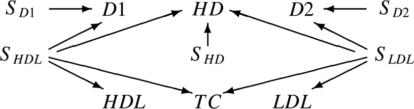
Let us illustrate this definition relative to figure 2, where $W=\{\mathrm{HDL},\mathrm{LDL},D1,D2,\mathrm{HD}\}$ and $I=\left\{\mathrm{TC}\right\}$ . (i) There is a shock for each variable in W. Some shocks (e.g., S _D1) only hit one variable (D1). Others are common to multiple variables. (ii) For any variable (e.g., HDL), its shock (S _HDL) also hits all of its descendants, if any (D1, HD). (iii) Any shock to a determinant of a variable I_i in I (e.g., S _HDL) also hits I_i (TC). (iv) If V contained a cause of a determinant of I_i (e.g., dairies, Da, which causes LDL), its shock (S _Da) would also hit I_i (TC).

Figure 2.

${𝒢}_V^{\mathrm{IC}}$ corresponding to the DAG 𝒢_V in figure 1.

One may also define 𝒢^IC relative to any subset O of variables in V, namely, ${𝒢}_O^{\mathrm{IC}}=〈O\cup S_O,{ℰ}_O^{\mathrm{IC}}〉$ . The set S _O is obtained by removing from S those shocks, which ℭ assigns to variables in W that are not in O, and by adding those shocks, which ℭ assigns to variables in W that are determinants of variables in $I\cap O$ . The set ${ℰ}_O^{\mathrm{IC}}$ is obtained by removing from ℰ^IC all of those edges whose tails are not in S _O . For any variable set O, we call “idiosyncratic” a shock to a variable X in ${𝒢}_O^{\mathrm{IC}}$ that is a parent of X and of no other variable. We may now define ill- and well-defined variables:

For instance, TC is well-defined in {Da, TC} because Da is neither a determinant of TC nor a descendant of a determinant of TC and vice versa. By contrast, TC is ill-defined in {HDL, TC} because HDL is a determinant of TC, and $S_{\mathrm{HDL}}\overline{)⫫}\mathrm{HDL}|\mathrm{TC}$ . Also, TC is ill-defined in {TC, D1} and {TC, HD} because D1 and HD are effects of determinants of TC, and (respectively) $S_{D1}\overline{)⫫}D1|\mathrm{TC}$ and $S_{\mathrm{HD}}\overline{)⫫}\mathrm{HD}|\mathrm{TC}$ . More generally, a variable I is ill-defined in O if and only if O also contains a variable Y among I’s determinants or their descendants, and ${𝒢}_{\{I,Y\}}^{\mathrm{IC}}$ contains no shock S_Y on I, Y, such that I screens off S_Y from Y in ℭ. This lack of screening off intuitively captures the idea that a manipulation of I with respect to Y is ambiguous. In turn, to explain the lack of screening off, we need the following proposition (proof in appendix):

We can also define a graph ${𝒢}_O=〈O,{ℰ}_O〉$ representing the structure over O, where ℰ_O consists of the following edges. First, 𝒢_O has a modified edge $X\Rightarrow Y$ if and only if there is a directed path $X\Rightarrow \cdots \Rightarrow Y$ in 𝒢_V , and no variable between X and Y is in O. Next, let the tail ⋄ of the arrow $X\diamond \to Y$ indicate that X is ill-defined in {X, Y}. Then, 𝒢_O has an edge $X\diamond \to Y$ for any 〈X, Y, Z〉 for which X, $Y\in O$ , $Z\in V$ , $Z\notin O$ , and 𝒢_V features a path $X\Leftarrow Z\to Y$ , unless ${𝒢}_O^{\mathrm{IC}}$ has a shock S common to X, Y for which $S⫫Y|X$ in ℭ, in which case $X\to Y$ is in 𝒢_O . Furthermore, 𝒢_O has a standard edge $X\to Y$ if 𝒢_V has a directed path from X to Y featuring standard edges → or modified edges ⇒, and no variable between X and Y is in O. Finally, 𝒢_O has a bidirected edge $X⟷Y$ if and only if 𝒢_V has an active path $X\leftarrow \cdots \leftarrow Z\to \cdots \to Y$ featuring standard or modified edges, and only X, Y on that path are in O. No further edges are in 𝒢_O .

Illustrated in relation to figure 1, 𝒢_{HDL,TC,LDL} is $\mathrm{HDL}\Rightarrow \mathrm{TC}\Leftarrow \mathrm{LDL}$ , and 𝒢_{HDL,LDL,HD} is $\mathrm{HDL}\to \mathrm{HD}\leftarrow \mathrm{LDL}$ . The two problematic structures with ill-defined variables from section 2, namely, 𝒢_{TC,D1,D2} and 𝒢_{Da,TC,D1}, are represented as, respectively, $D1\leftarrow \diamond \mathrm{TC}\diamond \to D2$ and $\mathrm{Da}\to \mathrm{TC}\diamond \to D1$ . Finally, let us define the notions of ill- and well-defined causes:

For instance, HDL is a well-defined cause of HD in {HDL, HD}.Footnote ⁴ By contrast, TC is an ill-defined cause of HD in {TC, HD}.

4. Identification

We now illustrate the applicability of our framework to detecting ill-defined variables and improving causal inference. We begin with a condition under which one may unambiguously identify ill-defined variables.

For instance, applied to $V^{\prime }=\{\mathrm{TC},D1,D2\}$ , this condition establishes that TC is an ill-defined common cause of D1 and D2 (i.e., $D1\diamond \leftarrow \mathrm{TC}\to \diamond D2$ ), since $D1⫫D2$ , $D1\overline{)⫫}\mathrm{TC}$ , $\mathrm{TC}\overline{)⫫}D2$ , $D1\overline{)⫫}D2|\mathrm{TC}$ , and ${𝒢}_{V^{\prime }}^{\mathrm{IC}}$ has no idiosyncratic shock to TC. Proposition 2 is easily generalizable to cases with more than two determinants.

If one observes no effects of independent determinants of the ill-defined variable; for instance, in $V^{″}=\{\mathrm{Da},\mathrm{TC},D1\}$ , the above condition is not applicable. Nonetheless, one may still reduce the ambiguity concerning ill-defined variables and partially recover the causal structure. To this end, let us assume that determinism induces dependencies (DD):

In other words, there are probabilistic dependencies between variables with deterministic assignments and their determinants. This assumption is only violated by canceling paths from determinants to determined variables. Its satisfaction requires (similarly to CFC) the absence of special parameterizations. For simplicity, we also assume that O contains no determinants of variables in O, such that ℰ_O contains no modified edges ⇒.Footnote ⁵ Then, one may identify well-defined variables:

For instance, Da (which, to recall, causes LDL but not HDL) is well-defined in V″, since (i) $\mathrm{Da}⫫D1$ , and (ii) ${𝒢}_{\{\mathrm{Da},\mathrm{TC}\}}^{\mathrm{IC}}$ contains a shock S common to Da, TC, such that $S⫫\mathrm{TC}|\mathrm{Da}$ , and no idiosyncratic shock to Da, from which one may infer $\mathrm{Da}\to \mathrm{TC}$ . Next, one can identify putative ill-defined variables:

For instance, TC and D1 are such that (i) $\mathrm{TC}\overline{)⫫}D1$ . Moreover, in ${𝒢}_{\{\mathrm{TC},D1\}}^{\mathrm{IC}}$ they are (ii) children of a common shock and (iii.a) children of idiosyncratic shocks. Therefore, TC and D1 qualify as putatively ill-defined. Assuming the absence of bidirected modified paths, 𝒢_{TC,D1} cannot be $\mathrm{TC}\Leftarrow \cdots \Rightarrow D1$ . Therefore, only three structures are possible, namely, $\mathrm{TC}\diamond \to D1$ , $\mathrm{TC}\leftarrow \diamond D1$ , and $\mathrm{TC}⟷D1$ . The ambiguity may be resolved by enlarging V″ until a sufficient set Z of common causes of TC, D1 is found that screens them off, or (given Z) the dependence between TC and D1 is oriented such that one is a well-defined cause of the other (i.e., $\mathrm{TC}\to D1$ or $\mathrm{TC}\leftarrow D1$ ), or enough effects of determinants of TC or D1 are observed as to remove the idiosyncratic shock on TC or D1, such that either $\mathrm{TC}\diamond \to D1$ or $\mathrm{TC}\leftarrow \diamond D1$ holds.

5. Conclusion

The problem of variable definition is known to be responsible for ambiguous manipulations. Furthermore, we showed that it can lead to mistaken causal inferences by standard constraint-based causal discovery methods. To address the problem, we introduced a novel representation framework suitable for structures including ill-defined variables, that is, the IC representation. We argued that recovering the IC representation can unambiguously identify ill-defined variables, under certain assumptions, or at least exclude that certain variables are ill-defined and consequently reduce the risk of mistakes. Given recent advances in statistical techniques (e.g., ICA) by which one may recover the IC representation, our proposal holds great promise. Therefore, we strongly invite further research on the subject.