Introduction
An earlier version of this paper was presented at the 55th European Microwave Conference and was published in its Proceedings [Reference Rius, Benedicto, Favennec and Guzmán Vélez1].
For over a century, coaxial transmission lines have been widely used in radio-frequency (RF) applications. This is a straightforward configuration in which a dielectric material electrically isolates two concentric conducting cylinders [Reference Herman and Espenschied2]. These structures support a transverse electromagnetic mode and thus exhibit a very wide bandwidth. In addition, coaxial lines offer a degree of freedom D/d in their transverse plane, where D and d denote the diameters of the outer shield and the central core, respectively. This allows different physical dimensions to be used while maintaining the same characteristic impedance. As a reminder, the characteristic impedance of a coaxial line is given by (1):
 \begin{equation}Z = \frac{1}{{2\pi }}\sqrt {\frac{{{\mu _0}}}{{{\varepsilon _0}{\varepsilon _r}}}} ln\left( {\frac{D}{d}} \right)\end{equation}
For coaxial resonators requiring high-quality factors, the dielectric medium is typically air [Reference Musonda and Hunter3, Reference Ruiz-cruz, Fahmi and Mansour4] or vacuum for space applications. In the latter case, it is essential to be able to adjust the gap dimension between the concentric conductors in order to prevent the multipactor effect [Reference Benedicto, Aouidad, Rius, Favennec, Martin-Guennou and Manchec5, Reference Benedicto, Rius, Bonizec, Favennec, Buitrago Bernal and Martin-Guennou6]. This phenomenon can be destructive and is primarily dependent on the frequency, the gap width, and the RF power level [Reference Vaughan7].
This work introduces a filter topology based on a single coaxial basic block that incorporates both resonator and coupling structure. In this way, each block has its own degree of freedom, enabling independent control of all parameters. This presupposes a clever way of connecting all the coaxial blocks. To illustrate this, two tubular coaxial band-pass stub filters, F24 and F39, are presented. They rely on an original interconnection approach that results in a highly compact design, making them particularly well-suited for space applications.
The paper is structured as follows. First, the interconnection principle used to connect the elementary coaxial building blocks is described. Then, the chosen filter topology is detailed, along with the design of the individual coaxial blocks, each combining a resonator and an impedance inverter. The two band-pass stub filters are then synthesized, simulated, manufactured, and measured. As these filtering structures are intended to space applications, their power-handling capability with respect to the multipactor effect is also evaluated. In this extended version of the paper, the power-handling analysis of the developed filters is extended through additional simulations at specific unfavorable frequencies, where the energy stored in the components reaches its maximum. To confirm the reliability and soundness of the proposed design approach, two second-order band-pass filters are implemented using building blocks from the F24 filter and then measured. The positioning of this work relative to the state-of-the-art is then discussed. The last two points (second-order filters and state-of-the-art review) are also specific to this extended version. Finally, conclusions and perspectives are presented.
Coaxial interconnection
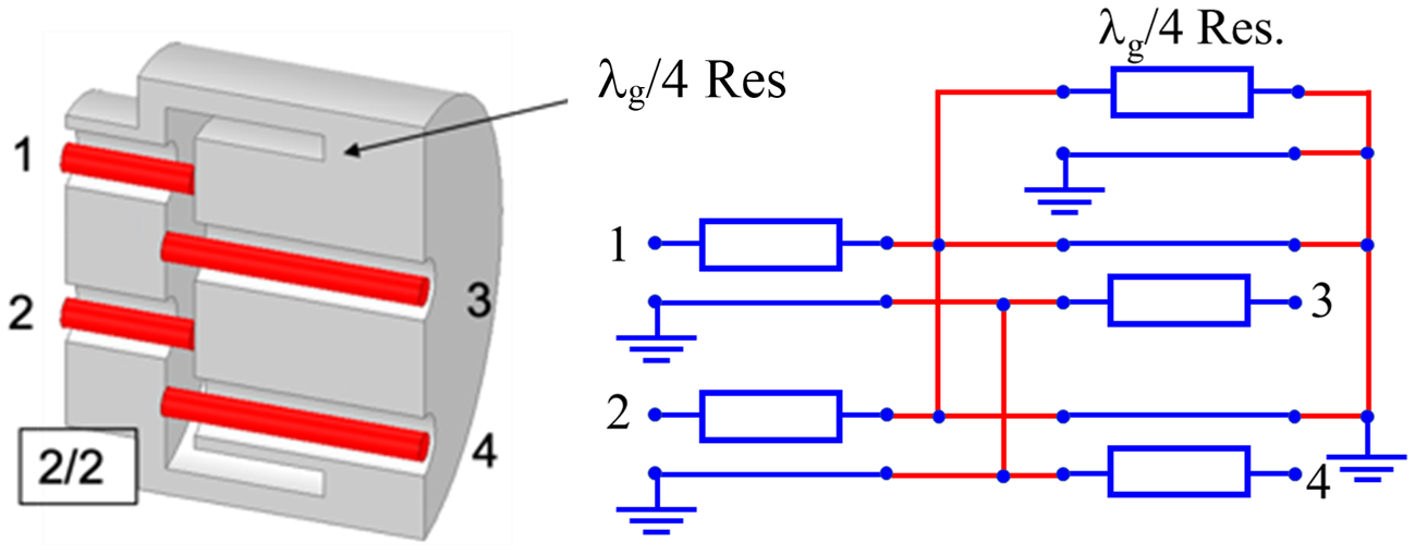
Figure 1 illustrates the basic idea, allowing the interconnection of multiple coaxial transmission lines. This is achieved by crossing the polarities of the conductors at the termination of a quarter-wavelength resonator. Consequently, the resulting interconnection is narrowband and centered around the resonant frequency of the resonator.
Interconnection 2/2 of four coaxial waveguides.

Figure 1 Long description
The diagram shows an interconnection of four coaxial waveguides labeled 1, 2, 3 and 4. Each waveguide is connected to a quarter-wavelength resonator labeled as lambda subscript f over 4 Res. The resonators are connected in a network with grounding symbols. Waveguide 1 is connected to a resonator, which is then connected to waveguide 3. Similarly, waveguide 2 is connected to a resonator, which is then connected to waveguide 4. The connections are made using lines that represent the conductors, with grounding points indicated at each waveguide connection. The resonators are positioned between the waveguides, facilitating the interconnection. The diagram visually represents the crossing of polarities at the termination of the resonators, allowing for narrowband interconnection centered around the resonant frequency.
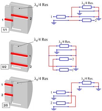
In the 2/2 configuration shown in Fig. 1, two lines from the left-hand side (n = 2) are connected to two lines from the right-hand side (m = 2) at the open end of a quarter-wavelength resonator. Such an implementation facilitates the interconnection of multiple coaxial lines. It has previously been exploited to develop innovative three-port coaxial combiners and dividers [Reference Rius, Benedicto, Favennec and Guzmán8]. In this form, this original connection [Reference Rius, Benedicto and Favennec9] is the generalization of a coupling system dedicated for a push–pull circuit [Reference Lindenblad10]. Figure 2 presents additional implementations of this concept when only two coaxial lines are considered. This is a particular case that can be declined in three possible configurations: 1/1, 0/2, and 2/0. For the stub filters investigated in this work, the 1/1 arrangement is selected. This configuration allows a coupling impedance inverter and a resonator to be designed within a concentric structure. Based on this, the elementary blocks of the filters will be constructed. The concentricity of the elements ultimately leads to compact, tubular filter structures.
Interconnections 1/1, 0/2, and 2/0 of two coaxial waveguides.

Figure 2 Long description
The image shows three configurations of coaxial waveguide interconnections with quarter-wavelength resonators. On the left, each configuration displays a physical cross-section of coaxial lines labeled 1 and 2. On the right, corresponding schematic diagrams illustrate the connections. In the 1/1 configuration, both lines 1 and 2 are connected to the resonator, labeled as lambda g over 4 resonator. In the 0/2 configuration, line 1 is open and line 2 connects to the resonator. In the 2/0 configuration, both lines are connected, but the resonator is not shown. Each schematic includes ground symbols and indicates the signal path. The layout flows from left to right, with ports 1 and 2 positioned at the top and bottom, respectively. The resonator is centrally located in each schematic, facilitating signal coupling and routing. Labels are expanded for clarity, ensuring screen reader compatibility.
Coaxial stub filter
Circuit model
By cascading the elementary building block N times, an Nth-order stub filter can be synthesized using established procedures in the literature [Reference Matthaei, Young and Jones11]. These topologies are particularly well suited to medium- and wide-band applications, where bandwidth is directly linked to the characteristic impedance values of the resonators, higher values leading to wider bandwidths.
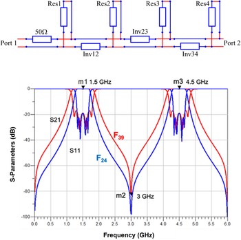
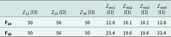
In this study, we have designed two fourth-order filters centered at F 0 = 1.5 GHz with relative bandwidths of 24% and 39%, denoted F24 and F39, respectively. Table 1 lists the required characteristic impedance values, where Zi ,i +1 and Z resi correspond to the characteristic impedance values of the inverters and resonators, respectively. Among the various possible solutions, we have selected inverters with characteristic impedances close to 50 Ω. All coaxial sections have identical lengths equal to λ g/4 at F 0, corresponding to 50 mm. Figure 3 shows the circuit model of the filter. It necessarily includes the 50 Ω access line, belonging to block 1, which does not contribute to the filtering function. Although the interconnection is incorporated in the model, its response is not different from that obtained with the conventional circuit. Figure 3 also displays the ideal electrical frequency responses of both filters. Note the first harmonic rise occurring at 3 × F 0.
Filter electrical model and electrical responses of F24 and F39 filters.

Figure 3 Long description
A composite figure with two parts. A) A circuit schematic with a horizontal main line from left to right. The left end is labeled Port 1 and the right end is labeled Port 2. A section near the left is labeled 50 ohm. Along the main line are three labeled elements: Inv12, Inv23 and Inv34. Four vertical branches connect upward from the main line to four rectangular elements labeled Res1, Res2, Res3 and Res4. B) A line graph with the y-axis labeled S-Parameters (decibel) and the x-axis labeled Frequency (gigahertz). The x-axis runs from 0.0 to 6.0 with labeled ticks every 0.5. The y-axis runs from 0 to minus 100 with labeled ticks at 0, minus 20, minus 40, minus 60, minus 80 and minus 100. Two curves are plotted: a red curve labeled F39 and a blue curve labeled F24. Text labels S21 and S11 appear near the left side of the plot. Four markers are labeled on the plot: m1 1.5 gigahertz near the left passband region, m2 3 gigahertz near a deep notch around the middle, m3 4.5 gigahertz near the right passband region and m4 4.5 gigahertz near the right passband region. The red and blue curves rise from near minus 100 decibel at low frequency toward higher values near the left passband around 1.5 gigahertz, then drop to a low region around 3 gigahertz, then rise again near 4.5 gigahertz and finally fall toward low values approaching 6.0 gigahertz.
Characteristic impedances of the various coaxial sections (inverters and resonators) of the filters

Table 1 Long description
The table lists characteristic impedances, in ohms, for three coaxial inverter sections and four resonator sections for two filters labeled F24 and F39. For both filters, the inverter impedances are identical: Z12 is 50 ohms, Z23 is 56 ohms, and Z34 is 50 ohms. Resonator impedances are lower in F24, with resonators 1 and 4 at 12.8 ohms and resonators 2 and 3 at 10.1 ohms. Resonator impedances are higher in F39, with resonators 1 and 4 at 23.4 ohms and resonators 2 and 3 at 19.6 ohms. In both filters, resonators 1 and 4 match each other, and resonators 2 and 3 match each other, indicating a symmetric resonator pattern. The main difference between the two filters is the resonator impedance level, not the inverter impedance values.
Physical model
The physical design of the filters requires fixing certain geometrical dimensions, primarily due to feasibility constraints. In particular, the diameter d 1 of the central cylinders and the thickness of the internal cylinders, (d 2 − D 1)/2, are set to 3 or 2.75 mm, and 2 mm, respectively.
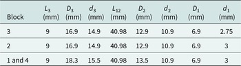
Using these values, along with Table 1 and Equation (1), the other transverse dimensions can be determined. Tables 2 and 3 present the main dimensions of the two filters, with the L 12 length fixed at 40.98 mm.
Main dimensions of the filter F24

Table 2 Long description
The table lists dimensional measurements in millimeters for three block configurations of the F24 filter: block 3, block 2, and the combined block 1 and 4. All configurations share the same L3 length of 9 mm and the same L12 length of 40.98 mm. Blocks 2 and 3 match across all listed diameters: D3 is 16.9 mm, d3 is 14.9 mm, D2 is 12.9 mm, d2 is 10.9 mm, and D1 is 6.9 mm. The combined block 1 and 4 is larger in the outer diameters, with D3 at 18.3 mm and D2 at 13.5 mm, and it also has a larger d3 at 15.5 mm, while d2 and D1 remain the same as the other blocks. The smallest inner diameter d1 differs by block: 2.75 mm for block 3, and 3 mm for block 2 and for block 1 and 4. Values are presented as nominal dimensions; manufacturing tolerances are not provided.
Main dimensions of the filter F39

Table 3 Long description
The table lists millimeter dimensions for filter F39 by block, including lengths L3 and L12 and diameters D3, d3, D2, d2, D1, and d1. Blocks 2 and 3 share identical values: L3 10.5, D3 21.3, d3 17.1, L12 40.98, D2 15.1, d2 10.9, and D1 6.9. Their only difference is d1, which is 2.75 for block 3 and 3 for block 2. Blocks 1 and 4 match each other and have larger D3 and d3 than blocks 2 and 3, at 23.3 and 18.1 respectively. Blocks 1 and 4 also have a larger D2 of 16.1, while d2 and D1 remain the same as the other blocks at 10.9 and 6.9. L3 and L12 are consistent across all blocks at 10.5 and 40.98. Values are presented as nominal dimensions in millimeters; no tolerances or measurement conditions are provided.
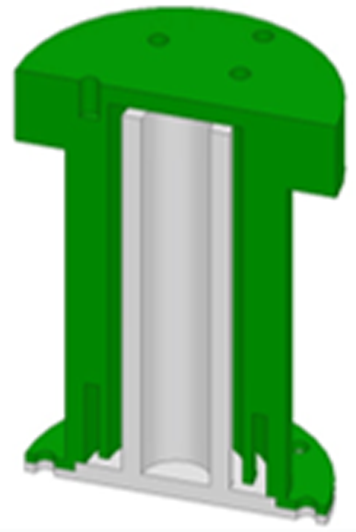
In all tables, the gray boxes refer to inverters. Figure 4(a) shows the cross-section of the first (or fourth) elementary block of the F24 filter, while Fig. 4(b) illustrates the cross-section of the first two blocks of the F24 filter, after assembly. For the filters to operate correctly, the inverters and resonators must have identical electrical lengths. However, the particular geometry of the interconnection and the associated electromagnetic discontinuities, especially at the terminations, introduce deviations that need to be corrected. This is achieved by adjusting the resonator length at its short-circuited end. For the F24 and F39 filters, the required additional lengths L 3 are 9 and 10.5 mm, respectively.
Cross-section of (a) An elementary block (block 1 or 4 of F24 filter). (b) Two assembled blocks (blocks 1 and 2 of F24 filter).

Figure 4 Long description
The image consists of two parts. The first part, labeled as (a), shows the cross-section of an elementary block of the F filter. It features a cylindrical structure with a height of 44.5 millimeters and a width of 32.3 millimeters. The block includes an inverter and a resonator, highlighted in different colors. The resonator is marked with segments labeled t1, t2, d1, d2, d3 and d4, indicating different sections along its length. The second part, labeled as (b), illustrates the cross-section of two assembled blocks of the F filter. The blocks are stacked vertically, with the top block labeled as Block 2 and the bottom as Block 1. The components include Inv12, Res2, Res1 and a 50 ohm section, with arrows pointing to each part. The resonator and inverter are shown in the same colors as in the first part and the additional length L3 is indicated at the bottom of the structure.
Quality factor and electromagnetic simulation
Although the relative bandwidth of the filters is important, evaluating the resonator’s quality factor is still essential. This can be achieved through eigen mode simulation of each elementary block, where the inverter function is removed by eliminating its central conductor. In this way, we retain a structure that is relatively close to the original one but operates purely as a resonator at the frequencies under consideration, as shown in Fig. 5. Assuming an electrical conductivity of aluminum of 38 × 106 S.m−1, the quality factor values range from 465 to 1050 (Table 4).
Simulation model of a resonator for evaluating the quality factor in eigen mode (block 1 or 4 of F24 filter).

Quality factors of the resonators

Table 4 Long description
The table reports resonator quality factor values for two block groupings, measured at two settings labeled F24 and F39. For block 2 and 3, the quality factor is 465 at F24 and 890 at F39. For block 1 and 4, the quality factor is 595 at F24 and 1050 at F39. At both settings, block 1 and 4 has higher quality factors than block 2 and 3. Both block groupings show higher quality factors at F39 than at F24. The labels F24 and F39 are not defined in the table, so the meaning of the settings and any measurement conditions are not specified.
The electromagnetic simulation can be carried out either on the full filter or on an elementary block. The results obtained are very similar. However, in terms of computational time and memory resources, the second solution is the most economical.
As shown in Fig. 6(a) and (b), circuit and electromagnetic simulation results are in very good agreement in the passband. Despite the deviations in the attenuated band due to discontinuity effects, the harmonic rise in the vicinity of 3 × F 0 is visible. The insertion losses at the center frequency are 0.2 and 0.12 dB for filters F24 and F39, respectively.
Electromagnetic and circuit simulations of the filters. (a) Filter F24. (b) Filter F39.

Figure 6 Long description
A) The plot has a y-axis labeled S-Parameters (decibel) with tick labels at 0, minus 20, minus 40, minus 60, minus 80 and minus 100. The x-axis is labeled Frequency (gigahertz) with tick labels from 0.0 to 6.0 in steps of 0.5. A legend shows Circuit simulation as a black dashed line and Electromagnetic simulation as a blue solid line. Text labels S21 and S11 appear near the left side. Marker labels appear as m1 0.2 decibel at 1.5 gigahertz, m2 3 gigahertz and m3 4.5 gigahertz. The blue solid curve rises from about minus 60 decibel near 0.0 gigahertz to near 0 decibel around 1.5 gigahertz, with several narrow downward spikes around the 1.5 gigahertz region. The curve then drops to a deep minimum near 3 gigahertz close to minus 100 decibel, then rises again toward near 0 decibel around 4.5 gigahertz with multiple narrow downward spikes in that region. Past about 5 gigahertz, the blue curve trends downward and then shows a sharp rise near the far right edge close to 6.0 gigahertz. The black dashed curve follows a similar overall shape, with closely spaced narrow dips around the 1.5 gigahertz and 4.5 gigahertz regions and a deep minimum near 3 gigahertz. B) The plot has a y-axis labeled S-Parameters (decibel) with tick labels at 0, minus 20, minus 40, minus 60 and minus 80. The x-axis is labeled Frequency (gigahertz) with tick labels from 0.0 to 6.0 in steps of 0.5. A legend shows Circuit simulation as a black dashed line and Electromagnetic simulation as a red solid line. Text labels S21 and S11 appear near the left side. Marker labels appear as m1 0.1 decibel at 1.5 gigahertz, m2 2.98 gigahertz and m3 4.5 gigahertz. The red solid curve rises from about minus 50 decibel near 0.0 gigahertz to near 0 decibel around 1.5 gigahertz, with several narrow downward spikes around the 1.5 gigahertz region. The curve then drops to a deep minimum near 2.98 gigahertz close to minus 80 decibel, then rises again toward near 0 decibel around 4.5 gigahertz with multiple narrow downward spikes in that region. Beyond about 5 gigahertz, the red curve shows large downward excursions, including a deep notch near the right side approaching the bottom of the axis and then rises again near 6.0 gigahertz. The black dashed curve follows a similar overall shape, including the rise near 1.5 gigahertz, the deep minimum near about 3 gigahertz and the rise near 4.5 gigahertz.
Manufacturing and experimental results
To experimentally validate the concept, both filters were fabricated from aluminum using conventional machining with a manufacturing tolerance of ±50 µm. The three parts of each elementary blocks, shown in Fig. 4(a), were manufactured separately and then assembled. Figure 7 shows a photograph of the different parts of block 1 of the F24 filter, before assembly.
Photograph of the three parts of block 1 of the F24 filter.

The experimental results are shown in Fig. 8(a) and 8(b). Despite some differences, mainly due to inter-block connection faults and manufacturing imperfections, especially for the F39 filter, the agreement with the simulation results is fairly good. For the F39 filter, the peak observed just below 3 GHz is attributed to a systematic defect in the resonator length, leading to desynchronization between the resonators and inverters; this defect can be rectified. It should be noted that no adjustment screws were provided. Measured insertion losses are 0.36 and 0.24 dB for F24 and F39 filters, respectively. A photograph of the F24 filter is presented in Fig. 8(c).
Experimental and electromagnetic responses of the filters. (a) Filter F24. (b) Filter F39. (c) Photograph of the F24 filter.

Figure 8 Long description
The image A showing a line graph with two overlaid curves and three marked points. The y-axis label is S-Parameters (decibel), ranging from 0 to minus 100. The x-axis label is Frequency (gigahertz), ranging from 0 to 5. A legend shows Measurement and Electromagnetic simulation. Two traces are plotted: a solid line for Measurement and a dashed line for Electromagnetic simulation. Text labels near the curves read S21 and S11. Marker m1 is labeled minus 0.36 decibel at 1.5 gigahertz. Marker m2 is labeled 3 gigahertz and is placed at the deepest notch near the bottom of the plot. Marker m3 is labeled 4.5 gigahertz and is placed near a high point close to 0 decibel. The curves rise from low values near the left side toward a high region near 1.5 gigahertz, then drop to a deep notch around 3 gigahertz, then rise again toward a high region near 4.5 gigahertz. The image B showing a line graph with two overlaid curves and three marked points. The y-axis label is S-Parameters (decibel), ranging from 0 to minus 100. The x-axis label is Frequency (gigahertz), ranging from 0 to 5. A legend shows Measurement and Electromagnetic simulation. Two traces are plotted: a solid line for Measurement and a dashed line for Electromagnetic simulation. Text labels near the curves read S21 and S11. Marker m1 is labeled minus 0.24 decibel at 1.5 gigahertz. Marker m2 is labeled 3 gigahertz and is placed at the deepest notch near the bottom of the plot. Marker m3 is labeled 4.5 gigahertz and is placed near a high point close to 0 decibel. The curves rise toward a high region near 1.5 gigahertz, then drop to a deep notch around 3 gigahertz, then rise again toward a high region near 4.5 gigahertz. The image C showing a rectangular metal assembly with four labeled sections. A horizontal dimension label above the object reads approximately 180 millimeter. A vertical dimension label at the right reads approximately 35.5 millimeter. Labels under the object read Block 4, Block 3, Block 2 and Block 1 from left to right.
Multipactor simulation
To evaluate the power handling of such filters in a space environment, multiphysics simulations were conducted using Spark3DTM [12]. The Total Electron Emission Yield characteristics [Reference Fil, Belhaj, Hillairet and Puech13] correspond to aluminum with a maximum secondary emission coefficient of δ = 2.98, a peak electron energy Em = 150 eV and a lower crossover electron energy E 1 = 24 eV. The initial number of electrons was set to 10 000. The multipactor thresholds obtained at the center frequency F 0 were 45 and 50 W, for F24 and F39 filters, respectively. For each filter, Fig. 9 shows the elementary charge distribution at F 0 for a power level slightly above the multipactor threshold. These illustrations, generated using Spark3DTM, demonstrate the locations of electron avalanches after 130 ns, in resonator 2, particularly near the interconnection region.
Elementary charge versus time for powers of 46 and 51 W per carrier, at a frequency of 1.5 GHz, for F24 and F39 filters.

Figure 9 Long description
The diagram consists of two sequences of images illustrating electron avalanches in resonators for two different filters, F24 and F39, over time. The top sequence shows four stages of electron distribution in a resonator for the F24 filter at 0 nanoseconds, 27 nanoseconds, 71 nanoseconds and 131 nanoseconds. At each stage, the distribution of electrons changes, culminating in a circular pattern at 131 nanoseconds. To the right, an inset shows the final electron distribution at 46 watts, labeled F24. The bottom sequence depicts a similar progression for the F39 filter at 0 nanoseconds, 50 nanoseconds, 120 nanoseconds and 200 nanoseconds. The electron distribution evolves over time, resulting in a circular pattern at 200 nanoseconds. An inset on the right shows the final distribution at 51 watts, labeled F39. Blue arrows indicate the progression of time between each stage in both sequences.
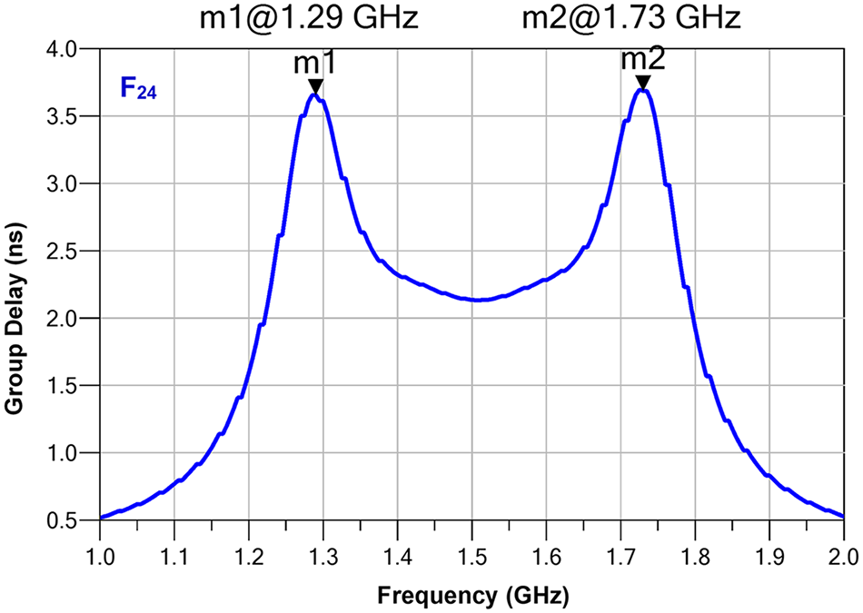
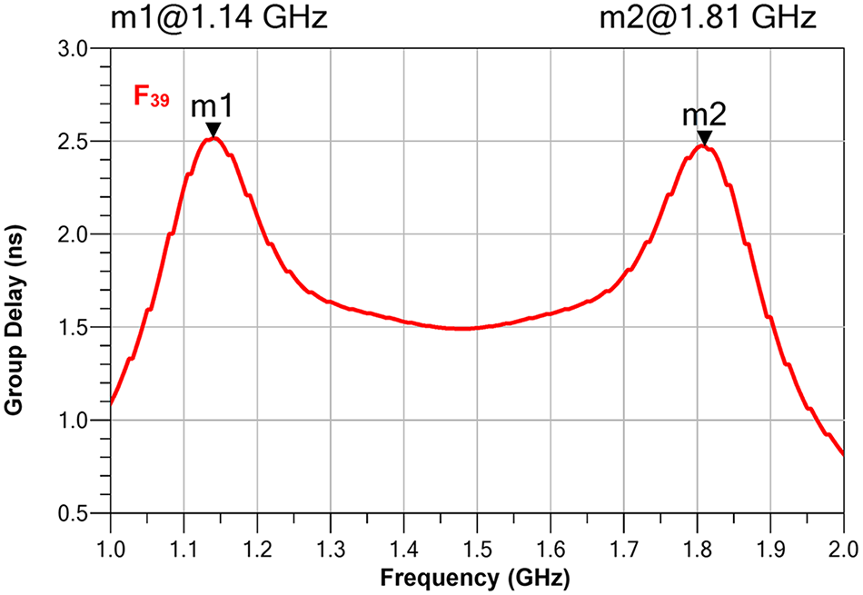
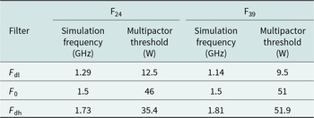
The stored energy in a filter reaches its maximum at frequencies F dl (low frequency) and F dh (high frequency), corresponding to the group delay maxima [Reference Ernst, Postoyalko and Khan14, Reference Yu15] (Figs 10, 11).
Electromagnetic simulation of the group delay response of the F24 filter.

Electromagnetic simulation of the group delay response of the F39 filter.

Thus, at the band-edge frequencies F dl and F dh, low multipactor thresholds are expected. Simulations performed at these frequencies confirm that, compared to F 0, this is true for F dl in both filters and for F dh in the F24 filter (Table 5). Concerning the F dh frequency of the F39 filter, the multipactor threshold is equivalent to that obtained at F 0. It is important to note that, for both filters, all electron avalanches at F 0, F dl, and F dh occur in resonator 2, as shown in Fig. 9.
Multipactor threshold at frequencies F 0, F dl, and F dh

Table 5 Long description
The table reports simulated multipactor threshold power in watts at three operating points (Fdl, F0, Fdh) for two filters, F24 and F39, along with the simulation frequency in gigahertz. For F24, thresholds are 12.5 W at 1.29 GHz (Fdl), 46 W at 1.5 GHz (F0), and 35.4 W at 1.73 GHz (Fdh). For F39, thresholds are 9.5 W at 1.14 GHz (Fdl), 51 W at 1.5 GHz (F0), and 51.9 W at 1.81 GHz (Fdh). Both filters have their lowest threshold at Fdl, and both share the same simulation frequency at F0. Comparing filters, F39 is lower than F24 at Fdl, higher at F0, and much higher at Fdh. Thresholds do not increase steadily with frequency for F24, while F39 rises from Fdl to F0 and remains high at Fdh. Values are simulation results and may differ from measured performance under different conditions.
These results are consistent with the relationship stating that the smaller the frequency–gap product F × D g, the lower the expected multipactor threshold [Reference Yu15], where F is the frequency of interest (F 0, F dl, and F dh) and D g the smallest gap between two metallic walls inside the filter.
Since D g is an intrinsic parameter of each filter, the lowest multipactor threshold is naturally observed at the lower frequency F dl. For the wideband filter F39, F dh is significantly higher than the center frequency F 0, leading to an equivalent multipactor threshold.
Discussion
The proposed filter architecture, where each block combines an isolated coaxial resonator and an impedance inverter, is highly compartmentalized. Consequently, the resonators are very well isolated from each other, enabling a clean integration without parasitic couplings. Moreover, non-adjacent parasitic couplings, which can be detrimental to high-order filters, are not an issue in this case.
Thus, using the building blocks of our fourth-order filter F24, several filters were quickly constructed Fig. 12(a), whose measurements are shown in Fig. 12(b) and (c).
(a) Second-order filters constructed by combining two blocks of the F24 filter. (b) Measurements Block 1 + Block 2 filter. (c) Measurements Block 1 + Block 4 filter.

Figure 12 Long description
The image A showing a cylindrical metal device lying horizontally on a flat surface. The device has a wider circular flange on the left end, two ring-like collars along the body and a smaller protruding connector on the right end. The label (a) appears below the device. The image B showing a line graph with the text “m1 -0.14 dB@1.5 GHz” above the plot. The y-axis label is “S-Parameters (dB)”. The y-axis ranges from 0 to minus 70 with tick marks every 10. The x-axis label is “Frequency (GHz)”. The x-axis ranges from 0.5 to 5.0 with tick marks every 0.5. Three curves are shown: a black curve labeled “F24”, a blue curve labeled “S21” and a red curve labeled “S11”. A marker “m1” is placed near 1.5 on the frequency axis at about minus 0.14 on the S-Parameters axis. The blue S21 curve forms a broad dip centered near 3.0 gigahertz, reaching close to minus 70 decibel at the minimum, then rises toward values near 0 decibel by about 4.5 to 5.0 gigahertz. The red S11 curve stays near 0 decibel for much of the range, with a dip near about 1.5 gigahertz and another dip near about 4.6 to 4.8 gigahertz. The black F24 curve runs close to 0 decibel across most of the frequency range. The text “Block 1 + Block 2” appears inside the plot area near the lower left. The image C showing a line graph with the text “m1 -0.12 dB@1.5 GHz” above the plot. The y-axis label is “S-Parameters (dB)”. The y-axis ranges from 0 to minus 70 with tick marks every 10. The x-axis label is “Frequency (GHz)”. The x-axis ranges from 0.5 to 5.0 with tick marks every 0.5. Three curves are shown: a black curve labeled “F24”, a blue curve labeled “S21” and a red curve labeled “S11”. A marker “m1” is placed near 1.5 on the frequency axis at about minus 0.12 on the S-Parameters axis. The blue S21 curve forms a broad dip centered near 3.0 gigahertz, reaching close to minus 70 decibel at the minimum, then rises toward values near 0 decibel by about 4.5 to 5.0 gigahertz. The red S11 curve stays near 0 decibel for much of the range, with a dip near about 1.5 gigahertz and another dip near about 4.6 to 4.8 gigahertz. The black F24 curve runs close to 0 decibel across most of the frequency range. The text “Block 1 + Block 4” appears inside the plot area near the lower left. The label (c) appears below the graph.
Without any adjustment, the measured passbands are highly satisfactory, with acceptable return loss, demonstrating excellent isolation between the blocks and resulting in predictable and controlled performances.
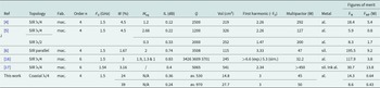
Table 6 provides a state-of-the-art overview of volumic microwave filtering solutions relevant to this work. To support performance assessment, we used two figures of merit, FM and FMp [Reference Bonizec, Benedicto, Favennec, Rius and Goujon16]. Despite their large bandwidth ratios W, which negatively impact these figures of merit, the proposed filters achieve very satisfactory performances, for a particular form factor.
Comparison “this work” with state-of-the-art solutions

Table 6 Long description
The table compares several resonator filter designs by topology, fabrication method, filter order, center frequency, fractional bandwidth, insertion loss, quality factor, volume, first harmonic location, multipactor power, metal, and two figures of merit. Most prior entries are machined stepped impedance resonators around 1.5 GHz with narrow bandwidths from about 1.67 to 4.5 percent, high quality factors from about 1200 to over 5000, and large volumes from about 115 to 541 cubic centimeters. The “this work” coaxial quarter wave design at 1.5 GHz stands out for bandwidth of 24 percent and a much smaller volume of 14.8 cubic centimeters, with insertion loss 0.36 dB and average quality factor about 530. Its first harmonic is listed at three times the center frequency and multipactor power at 45 W, which is lower than the entry reporting above 450 W but similar to the lowest reported values around 32 to 47 W. In figures of merit, the highest FM appears in reference 6 at 195.5, while “this work” reports FM 14.3 and FMP 0.64, below several SIR designs. A second line associated with “this work” reports bandwidth 39 percent, insertion loss 0.24 dB, average quality factor about 970, volume 27.7 cubic centimeters, first harmonic three times, multipactor 50 W, and FM 8.6 with FMP 0.43. Some cells are missing or mixed between measured and simulated values, so direct comparisons may be limited where data are not reported consistently.
exp. = measurements, sim. = simulation, mac. = machining, Fab. = fabrication, sil. = silver, al. = aluminum, cu. = copper, av. = average.
Conclusion
This work demonstrates the design of tubular coaxial stub filters, dedicated to medium and wideband applications. This was achieved using an original interconnection technique based on crossing the polarities of the metallic conductors of the quarter-wavelength coaxial resonators and those of the admittance inverters. Two filter prototypes were designed and experimentally validated, showing good agreement with simulations. Through simulations performed using Spark3DTM, we analyzed the multipactor power handling of each filter. These analyses, performed at three specific frequency points, the center frequency and the frequencies of maximum stored energy (i.e., where the group delay is maximum), produced consistent results. By combining two blocks from the fourth-order F24 filter, two second-order filters were constructed without any tuning. The resulting responses were highly satisfactory, demonstrating an excellent isolation between the two blocks and confirming the reliability and the soundness of the proposed design approach. Finally, a state-of-the-art overview of volumic filtering solutions shows that the proposed design approach provided a good compromise between electrical performance, compactness, and power handling, for a particular form factor. Now that the principle has been validated, it remains to be determined how lower bandwidths can be achieved. One possible improvement would be to remove the 50 Ω line from block 1, which is unnecessary. An in-depth study on power handling also remains to be conducted. This study should be based on the degrees of freedom offered by each of the basic building blocks of the filter, bearing in mind that resonators and inverters do not exhibit the same electrical behaviors.
Acknowledgements
The authors would like to thank the company Breizh Usinage Service (Pleyben, France) for manufacturing the filters, Gael Leroux (Université de Brest, France) for its help in assembling the filters, and the SATT Ouest Valorization and FRAME xG (FRench progrAm of IP Massification for Europe in XG) for supporting the work.
Competing interests
The authors declare none.

Juan Pablo Guzman Velez was born in Bogota, Colombia, in 1982. He received the B.Sc. and M.Sc. degrees in electronic engineering from the Universidad Nacional de Colombia in 2008. He worked then, toward his Ph.D. degree in electronic engineering in Telecom Bretagne, Plouzané, France, which he obtained in 2013. His doctoral thesis dealt with the integration of antenna and active devices for 60 GHz radios. He is currently a Post-Doctoral Researcher with the Lab-STICC, University of Brest. His research interests include design of passive components for microwave.

Eric Rius (Senior Member, IEEE) is currently a professor at the University of Brest, Brest. He was the Vice-Head of the Laboratoire des Sciences et Techniques de l’Information, de la Communication et de la Connaissance (Lab-STICC), Brest, France, from 2016 to 2020. His research conducted at Lab-STICC concerns the design of passive microwave devices for centimetric and millimetric-wave applications. He spent several months in Singapore as a Visiting Professor at Nanyang Technological University. He is involved in many projects with the three French agencies, Agence Nationale de la Recherche (ANR), Direction générale de l’Armement (DGA), and Centre national d’études spatiales (CNES), and companies, such as Thales Alenia Space, Toulouse, France.

Jessica Benedicto (Member, IEEE) received the Ph.D. degree in physics from Blaise Pascal University, Clermont-Ferrand, France, in 2013. During her Ph.D. degree, she investigated the potential of metallodielectric multilayers, flat lenses with subwavelength resolution, and nonlocality in metals. In 2013, she held a post-doctoral position at the Fresnel Institute, Marseille, France. The fields of application of her post-doctoral research were hybrid magnetic–electric dielectric scatterer near- and far-field analyses. In 2015, she became an assistant professor at the University of Brest, Brest, France. She currently conducts research at the Laboratoire des Sciences et Techniques de l’Information, de la Communication et de la Connaissance (Lab-STICC), Brest. Her research interests concern the modeling and design of passive devices for microwave applications.

Jean-François Favennec received the Ph.D. degree in electronics from the University of Brest, Brest, France, in 1990, and the Accreditation to Supervise Research (HDR), University of Brest in 2016. He is currently a professor with the Ecole Nationale d’Ingenieurs de Brest, Plouzané, France. He mainly teaches electromagnetic theory and microwaves. He conducts research at the Laboratoire des Sciences et Techniques de l’Information, de la Communication et de la Connaissance (Lab-STICC), Brest. His current research focuses on the modeling and design of passive devices for microwave applications, mainly focusing on filters.