1. Introduction
An interaction of the reaction–diffusion processes and hydrodynamics has always attracted various researchers to explore the chemo-hydrodynamic instabilities (De Wit, Eckert & Kalliadasis Reference De Wit, Eckert and Kalliadasis2012; De Wit Reference De Wit2016). One such interaction is observed during fingering instabilities involving reactive fluid–fluid interfaces. The displacement of a more viscous fluid by a less viscous one in a porous medium results in an instability called viscous fingering (VF) (Tan & Homsy Reference Tan and Homsy1986; De Wit Reference De Wit2016). When the fluids are miscible in nature, the forces due to convection and diffusion compete as diffusion tends to stabilise the system (Tan & Homsy Reference Tan and Homsy1986; Sharma et al. Reference Sharma, Nand, Pramanik, Chen and Mishra2020). In addition, if the fluids are reactive then a coupling between convection, diffusion and the chemical reaction affects the overall dynamics. Understanding VF induced by chemical reaction helps us to understand the effect of the forces due to convection, diffusion and reaction, and to analyse which force dominates which dynamics. Moreover, the chemical reaction destabilises the system and enhances the mixing (Gérard & De Wit Reference Gérard and De Wit2009; Sharma et al. Reference Sharma, Pramanik, Chen and Mishra2019). Hence, VF induced by chemical reaction can be utilised for increasing mixing in a variety of fields ranging from macro-scale in chemical, pharmaceutical and food processing industry (Jha, Cueto-Felgueroso & Juanes Reference Jha, Cueto-Felgueroso and Juanes2011a) to micro-scale in microfluidic devices (Jha, Cueto-Felgueroso & Juanes Reference Jha, Cueto-Felgueroso and Juanes2011b, Reference Jha, Cueto-Felgueroso and Juanes2013). Further, VF has applications in the point-of-care devices (Clingan et al. Reference Clingan, Rusk, Smith and Garcia2018) and provides a mean to test urea using saliva (Cardoso et al. Reference Cardoso, Arregger, Tumilasci, Elbert and Contreras2009). The pattern formation is useful for various medical diagnosis kits (Sett et al. Reference Sett, Ayushman, Dasgupta and DasGupta2018), in biomedical applications and tissue spreading (Bogdan & Savin Reference Bogdan and Savin2018). Usually, reactive fluids are utilised with the involved reaction being instantaneous. Thus, a theoretical knowledge of effect/control of VF using chemical reaction is required and will be beneficial for multiple disciplines including chemistry, geophysics, geology, fluid dynamics and mathematics.
The chemical reaction can affect VF in a variety of ways which have been explored extensively in the literature. Two kinds of displacements are used to understand VF. One being the rectilinear displacement where one fluid displaces the other fluid uniformly and the other is the radial displacement. Both the displacements have basic differences which affect the overall VF dynamics. In radial flow, growth of perturbations is algebraic unlike the exponential growth in the rectilinear displacement (Tan & Homsy Reference Tan and Homsy1986). In addition, generation of more product for the radial case is reported (Brau & De Wit Reference Brau and De Wit2020) due to an increase in the contact zone between reactants with time. Thus, the kind of displacement considered has a significant effect on the VF dynamics. However, a linear displacement of one fluid by another is considered in majority of the theoretical studies, whereas the experiments utilise a radial displacement. Various experimental studies involve fluids undergoing neutralisation reactions which are an example of instantaneous reaction as the reaction rate is very large for such reactions. (Nagatsu & Ueda Reference Nagatsu and Ueda2001, Reference Nagatsu and Ueda2004; Nagatsu et al. Reference Nagatsu, Matsuda, Kato and Tada2007). Nagatsu et al. (Reference Nagatsu, Matsuda, Kato and Tada2007) experimentally showed the effect of an instantaneous chemical reaction on VF by considering radial displacement of the reactive as well as non-reactive fluids. They observed widening of the fingers for the reactive case when viscosity is increased by the chemical reaction, whereas the shielding effect is more than the non-reactive case when the chemical reaction decreases the viscosity. In another study, Nagatsu et al. (Reference Nagatsu, Kondo, Kato and Tada2009) explored the effect of the reaction rate on miscible VF involving radial displacement of the reactive fluids, in terms of a non-dimensional parameter Damköhler number  $Da$ defined as the ratio of the convective time scale to the reactive time scale. They reported the dynamics for moderate
 $Da$ to be different than those for a sufficiently high
 $Da$ (Nagatsu et al. Reference Nagatsu, Matsuda, Kato and Tada2007) signifying a dependence of the fingering dynamics on the reaction rate. In addition to these experimental studies, many theoretical studies (Gérard & De Wit Reference Gérard and De Wit2009; Hejazi & Azaiez Reference Hejazi and Azaiez2010; Hejazi et al. Reference Hejazi, Trevelyan, Azaiez and De Wit2010; Nagatsu & De Wit Reference Nagatsu and De Wit2011; Sharma et al. Reference Sharma, Pramanik, Chen and Mishra2019) have been conducted to understand reactive miscible VF. Hejazi et al. (Reference Hejazi, Trevelyan, Azaiez and De Wit2010) performed a linear stability analysis of miscible reactive system using quasi-steady-state approximation and analysed the effect of the non-monotonicity in the viscosity profile introduced by the chemical reaction on VF. Using a pseudo-spectral method, Hejazi & Azaiez (Reference Hejazi and Azaiez2010) studied VF due to a chemical reaction between reactants having viscosity different than the generated product and observed the rate of generation of the product decreases with an increase in the Péclet number.
The effect of an infinite  $Da$ on the VF dynamics is explored numerically by Nagatsu & De Wit (Reference Nagatsu and De Wit2011) where the chemical reaction modifies the viscosity in the system undergoing rectilinear displacement. However, owing to the difference in the displacement used in the simulations as well as in the experiments opposite trends in experimental finger width (Nagatsu et al. Reference Nagatsu, Matsuda, Kato and Tada2007) are obtained. The effect of chemical reaction between reactants having the same viscosity but producing a more viscous product is understood by Gérard & De Wit (Reference Gérard and De Wit2009). They succeed to explain the experimental observations of Podgorski et al. (Reference Podgorski, Sostarecz, Zorman and Belmonte2007) in terms of the diffusion coefficient and the initial concentration of the reactants. However, they do not discuss the VF dynamics when reaction produces a less viscous product than the reactants. This gap in literature was filled by Sharma et al. (Reference Sharma, Pramanik, Chen and Mishra2019) who discussed VF induced by chemical reaction by considering reactants having the same viscosity but generating a more and less viscous product. They discussed the dynamics for a range of finite
 $Da$ by considering radial displacement and obtained qualitative agreement with experiments (Podgorski et al. Reference Podgorski, Sostarecz, Zorman and Belmonte2007; Riolfo et al. Reference Riolfo, Nagatsu, Iwata, Maes, Trevelyan and De Wit2012). Further, for a given
 $Da$, the existence of critical viscosity contrast for the occurrence of VF is reported. However, the VF induced solely by an instantaneous chemical reaction between the reactants having the same viscosity is unexplored. In this work, we explore whether the critical viscosity contrast still exists when the reaction rate is infinite. We numerically discuss reactive fingering dynamics for the limiting case
 $Da \rightarrow \infty$ for reactants undergoing radial displacement. We suitably modify the governing equations to take care of
 $Da \rightarrow \infty$ similar to the work of Nagatsu & De Wit (Reference Nagatsu and De Wit2011) and Michioka & Komori (Reference Michioka and Komori2004). We gain insight into the effect and the interaction of the forces due to convection, diffusion and reaction on VF in terms of the dimensionless parameters and see whether the stable displacement still exists when the chemical reaction is infinitely fast. The stable displacement, if it exists, implies that force due to the reaction is not sufficient to overcome the other two forces due to convection and diffusion. Thus, the triggering of the instability also depends upon log mobility ratio,
 $R_c$, and the Péclet number,
 $Pe$, which are a measure of other two forces in the system. Hence, we determine the onset of instability in terms of these non-dimensional numbers. We obtain a relation of onset time of instability with log mobility ratio and the Péclet number which can be used to quantify the displacement as completely stable or having a finite time stability regime. Thus, using
 $R_c$, one can characterise the reactants so as to have a delayed or no instability as per the application. Further, we discuss the length of fingers when
 $t_{on}$ is finite, in order to gain insight into the mixing due to chemical-reaction-induced VF. The length of the fingers is found to have a non-monotonic dependence on the sign of
 $R_c$.
The article is organised as follows. The governing equations are discussed in § 2 followed by modifying the equations to deal with  $Da \rightarrow \infty$ in § 3. We discuss the results in terms of the onset of instability and finger length in § 4, followed by conclusions in § 5.
2. Mathematical formulation
We consider two fluids  ${A}$ and
 ${B}$ as reactants undergoing a second-order chemical reaction
 \begin{equation} A+B \rightarrow C, \end{equation}
upon contact to generate another fluid  ${C}$ as the product. The fluid
 ${A}$ radially displaces fluid
 ${B}$ in a two-dimensional homogeneous and isotropic porous medium having constant permeability
 $\tilde {\kappa }$. We consider the fluids to be miscible and the reactants have the same viscosity
 $\tilde {\mu }_0$, whereas the viscosity of the product
 $\tilde {\mu }_c$ may be different than the reactants. Considering the fluids to be incompressible and neutrally buoyant, we use a system of coupled nonlinear partial differential equations (PDEs) (Sharma et al. Reference Sharma, Pramanik, Chen and Mishra2019) to model the flow of reactive fluids in the porous medium. The system of PDEs comprises a continuity equation and the Darcy's law for the conservation of mass and momentum of the flow through porous medium, coupled to three convection–diffusion–reaction (CDR) equations for the mass balance of the three fluids
 $A$,
 $B$ and
 $C$. The non-dimensional governing equations are
 $$\begin{gather} \boldsymbol{\nabla} \boldsymbol{\cdot} \boldsymbol{u}=0, \end{gather}$$
 $$\begin{gather}\boldsymbol{\nabla} p={-}\mu(c) \boldsymbol{u}, \end{gather}$$
 $$\begin{gather}\frac{\partial a}{\partial t}+\boldsymbol{u} \boldsymbol{\cdot} \boldsymbol{\nabla} a=\frac{1}{Pe}\nabla^2a -Da \, ab, \end{gather}$$
 $$\begin{gather}\frac{\partial b}{\partial t}+\boldsymbol{u} \boldsymbol{\cdot} \boldsymbol{\nabla} b=\frac{1}{Pe}\nabla^2b - Da \, ab, \end{gather}$$
 $$\begin{gather}\frac{\partial c}{\partial t}+\boldsymbol{u} \boldsymbol{\cdot} \boldsymbol{\nabla} c=\frac{1}{Pe}\nabla^2c + Da \, ab, \end{gather}$$
where  $\boldsymbol {u}=(u,v)$,
 $p$ and
 $\mu$ denote the dimensionless Darcy velocity, pressure and viscosity, respectively. The non-dimensional chemical concentrations of the fluids
 ${A,B,C}$ are
 $a,b,c$, respectively. The above equations are obtained using a combination of the flow rate per unit depth
 $\tilde {Q}$ and total time for which fluid
 ${A}$ is injected
 $\tilde {t}_f$ as characteristic scales (Sharma et al. Reference Sharma, Pramanik, Chen and Mishra2019) as
 $$\begin{gather} \boldsymbol{x}=\frac{\tilde{\boldsymbol{x}}}{\sqrt{\tilde{Q} \tilde{t}_f}}, \quad \boldsymbol{u}= \frac{\tilde{\boldsymbol{u}}}{\sqrt{\tilde{Q}/ \tilde{t}_f}},\quad t=\frac{\tilde{t}}{\tilde{t}_f}, \end{gather}$$
 $$\begin{gather}(a, b, c)=\frac{(\tilde{a},\tilde{b},\tilde{c})}{\tilde{a}_0}, \quad \mu=\frac{\tilde{\mu}}{\tilde{\mu}_0}, \quad p=\frac{\tilde{p}}{\tilde{Q}\tilde{\mu}_0/\tilde{\kappa}}, \end{gather}$$
where dimensional quantities are represented with a tilde. The initial dimensional concentration of the reactant  ${A}$ is
 $\tilde {a}_0$. The viscosity–concentration relation is taken here as
 \begin{equation} \mu(c)={\rm e}^{R_c c},\quad R_c=\ln\left(\frac{\mu_c}{\mu_0}\right), \end{equation}
where  $\mu _0$ and
 $\mu _c$ are viscosities of the reactants and product, respectively and
 $R_c$ is the log-mobility ratio. Here, we encounter two more dimensionless parameters: the Damköhler number
 $Da$ and the Péclet number
 $Pe$ defined as
 \begin{equation} Da=\frac{\tilde{t}_f}{1/\tilde{k}\tilde{a}_0}, \quad Pe=\frac{\tilde{Q}}{\tilde{D}}, \end{equation}
where  $\tilde {k}$ is the reaction rate constant. We assume the three fluids have the same diffusion coefficient
 $\tilde {D}$ and, hence, only one
 $Pe$ appears in all three CDR equations. The Péclet number is the ratio of the mass transfer owing to convection and diffusion, whereas the Damköhler number being the ratio of convective time scale to reactive time scale depicts the relative importance of convection to that of reaction. As viscosity also contributes to the velocity of the fluid, we regard the log-mobility ratio as a measure of force due to convection. Thus, the three non-dimensional parameters actually provide a measure of the relative dominance of one of the three forces each due to convection, diffusion and reaction. As
 $Da \rightarrow \infty$ in this study, the force due to reaction is sufficiently large and the absence or presence of any instability is due to the dominance of the other two forces due to convection and diffusion which we discuss by varying
 $R_c$ and
 $Pe$ in § 4.
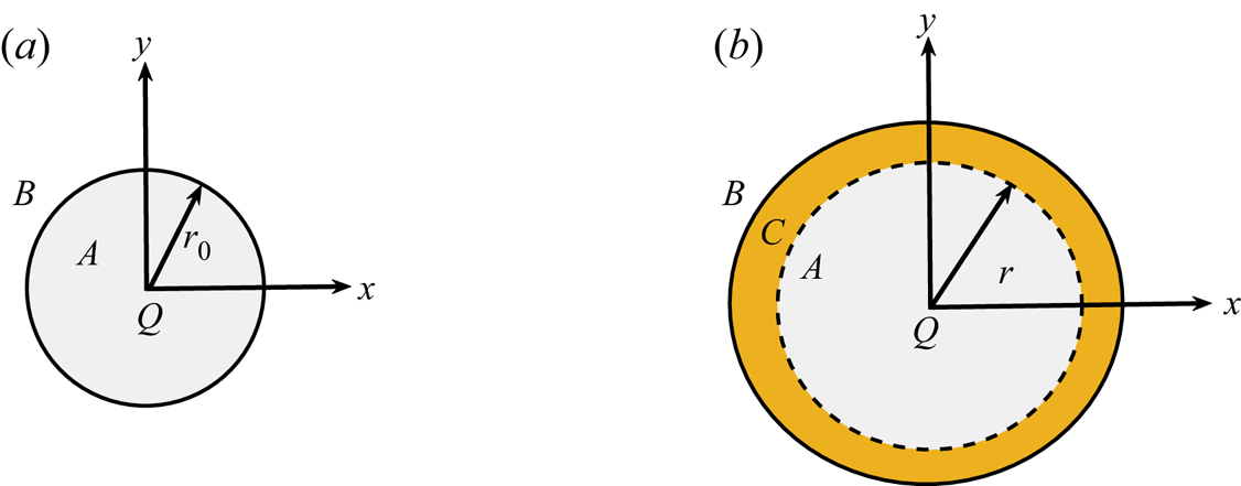
The fluid  ${A}$ is contained in a circle of non-dimensional radius
 $r_0$ initially and is surrounded by the fluid
 ${B}$ (see figure 1a). The fluid
 ${A}$ injected continuously with flow rate per unit depth
 $Q$ from the injection hole located at the origin. The fluid
 ${A}$ radially displaces fluid
 ${B}$ and both fluids undergo a chemical reaction to produce
 ${C}$ in the region between the reactants as shown in figure 1(b). Thus, the initial conditions associated with (2.2c)–(2.2e) are
 \begin{equation} (a,b,c)(x,y, t=0)=\begin{cases} (1,0,0) & x^2+y^2\leq r_0^2,\\ (0,1,0), & \mbox{otherwise,} \end{cases} \end{equation}
where  $r_0$ is the radius of the circular region initially filled with fluid
 ${A}$. We discuss the boundary conditions in the next subsection where we describe the numerical scheme used to solve the governing system of equations.
(a) Schematic of the problem at  $t=0$ showing reactant
 $A$ contained in a circle of radius
 $r_0$. The region outside the circle is occupied by reactant
 $B$. (b) Same schematic at
 $t>0$ depicting the generation of the product
 ${C}$ in the yellow coloured annulus region where the reactants come in contact. Here,
 $r > r_0$.

3. Numerical scheme
We perform numerical computations in Cartesian coordinates by considering a square computational domain with the injection hole being at the origin of the coordinate system. For numerical computations, we choose a non-dimensional domain  $\varOmega =[-L/2,L/2]\times [-L/2,L/2]$. In this study, we take
 $L=1.5$ and the domain is discretised into
 $n_x \times n_y$ grid points (see Appendix A for grid independence study). Further,
 $r_0=0.075$ throughout this study. There are a few challenges in performing a computational study of radial displacement of reactants undergoing an infinitely fast reaction. We have to deal with a singularity at the origin in the velocity field (Chen et al. Reference Chen, Huang, Gadêlha and Miranda2008; Sharma et al. Reference Sharma, Pramanik, Chen and Mishra2019) along with taking care of
 $Da$ which approaches infinity. We discuss these two before discussing the numerical method.
As we can see that  $Da$ appears in all three CDR equations (2.2c)–(2.2e), hence, in order to numerically deal with infinitely fast reaction rate (
 $Da\rightarrow \infty$), we must wisely modify the equations. We observe that simply adding or subtracting two of the CDR equations can help eliminate
 $Da$ from the equations. Hence, we add (2.2c) and (2.2e), and (2.2d) and (2.2e), to obtain the following two equations:
 $$\begin{gather} \frac{\partial H_1}{\partial t}+\boldsymbol{u} \boldsymbol{\cdot} \boldsymbol{\nabla} H_1=\frac{1}{Pe}\nabla^2 H_1, \end{gather}$$
 $$\begin{gather}\frac{\partial H_2}{\partial t}+\boldsymbol{u} \boldsymbol{\cdot} \boldsymbol{\nabla} H_2=\frac{1}{Pe}\nabla^2 H_2, \end{gather}$$
where  $H_1=a+c$ and
 $H_2=b+c$. It must be noted that now we have two convection–diffusion equations (3.1), one for each
 $H_i$,
 $i=1,2$, satisfying two different initial conditions (
 $H_1(x,y,t=0)= a(x,y,t=0)$ and
 $H_2(x,y,t=0)= b(x,y,t=0)$ as
 $c(x,y,t=0)=0$), whereas each satisfies no flux boundary condition. Further, by using a suitable normalisation (Nagatsu & De Wit Reference Nagatsu and De Wit2011),
 \begin{equation} h_i=\frac{H_i-H_{i;B_0} }{ H_{i;A_0}-H_{i;B_0} }, \quad i=1,2, \end{equation}
we show that we only need to solve one convection–diffusion equation. For  $i=1,2$, we denote normalised
 $H_i$ as
 $h_i$. Here,
 $H_{i;B_0}$ is the value of
 $H_i$ inside the region of displaced fluid and
 $H_{i;A_0}$ is the value of
 $H_i$ in the region of displacing fluid, that is,
 $$\begin{gather} H_{1;B_0}=0,\quad H_{2;B_0}=1, \end{gather}$$
 $$\begin{gather}H_{1;A_0}=1,\quad H_{2;A_0}=0. \end{gather}$$
Substituting the values of  $H_{i;B_0}$ and
 $H_{i;A_0}$ into (3.2), we obtain the value of
 $h_i$,
 $i=1,2$, as
 \begin{equation} h_1=a+c, \quad h_2=1-(b+c). \end{equation}
It is evident that both  $h_1, h_2$ now satisfy following two convection–diffusion equations
 \begin{equation} \frac{\partial h_i}{\partial t}+\boldsymbol{u} \boldsymbol{\cdot} \boldsymbol{\nabla} h_i=\frac{1}{Pe}\nabla^2 h_i, \quad i=1,2, \end{equation}
associated with the same following initial condition for both the equations
 \begin{equation} h_i(x,y, t=0)=\begin{cases} 1, & x^2+y^2\leq r_0^2 \\0, & \mbox{Otherwise} \end{cases}, \quad \mbox{for}\ i=1,2. \end{equation}
Thus, in place of solving two different equations each for  $h_i,i=1,2$, we can denote
 $h_1=h_2=h$ and solve the following differential equation for
 $h$
 \begin{equation} \frac{\partial h}{\partial t}+\boldsymbol{u} \boldsymbol{\cdot} \boldsymbol{\nabla} h=\frac{1}{Pe}\nabla^2 h, \end{equation}
associated with the initial condition (3.7) with  $h_i$ replaced with
 $h$. It is not possible to find the solution of the above equation using similarity variables (Sharma et al. Reference Sharma, Nand, Pramanik, Chen and Mishra2020). Thus, we solve the above equation numerically as explained ahead. The computed
 $h$ value is used to find the concentration
 $a,b,c$ (see Nagatsu & De Wit Reference Nagatsu and De Wit2011, and references therein), as explained in the following.
When we consider the chemical reaction to be infinitely fast, that is,  $Da \rightarrow \infty$, the reactive time scale,
 $1/ \kappa a_0$ becomes very small such that it is negligible in comparison with the convective time scale. Introducing such small time steps in simulations is quite difficult. To avoid such circumstances, we opt for a conserved scalar approach to handle this infinitely fast reaction. It must be noted that this approach can be utilised for infinitely fast reaction only, not for moderately fast reaction (Cook & Riley Reference Cook and Riley1994; Michioka & Komori Reference Michioka and Komori2004). To obtain
 $a,b,c$ from
 $h$, we utilise the fact that the reaction occurs with an infinite reaction rate. The region where both the reactants co-exist and, thus, react to generate the product is termed the reaction front. However, as
 $Da\rightarrow \infty$, the two reactants are consumed as soon as they come in contact and concentration of both the reactants tends to zero in the reaction front (Nagatsu & De Wit Reference Nagatsu and De Wit2011). See Appendix B for details. Thus, using (3.5a,b), we obtain that in the reaction front
 $c=h=0.5$. The two reactants cannot co-exist outside the reaction front, that is, when
 $h\neq 0.5$. Thus, for
 $h<0.5$, we have
 $a=0$ and we get from (3.5a,b) that
 $b=1-2h, c=h$. Similarly, for
 $h>0.5$ and
 $b=0$, we obtain
 $a=2h-1, c=1-h$ (see Appendix B for details). Thus, solving only one convection–diffusion equation (3.8) for
 $h$, we can obtain the reactant and the product concentration as
 \begin{equation} (a,b,c)=\begin{cases} (0,1-2h,h), & h<0.5,\\ ({-}1+2h,0,1-h), & h \geq 0.5. \end{cases} \end{equation}
It must be noted that there exist two more choices of  $H_1, H_2$ and thus obtained
 $h_1, h_2$ are different than used here (see Appendix C for details). However, we obtain the same (3.9) in each case. Thus, in order to deal with
 $Da\rightarrow \infty$, we actually simplified the situation by having to deal with only one convection–diffusion equation in place of three CDR equations. It is mentioned that the above method is applicable even when the initial concentration of the reactants is unequal. We define
 $\phi =b_0/a_0$ as the ratio of the initial concentration of the two reactants. Throughout this paper, we take
 $\phi =1$ but for
 $\phi \neq 1$, (3.3a,b)–(3.5a,b), (3.9) will be modified to include
 $\phi$. Now, we explain about resolving the singularity in the velocity field.
In the absence of any viscosity gradient, the radial flow is a potential flow with the velocity given as
 \begin{equation} \boldsymbol{u}_{pot}(x,y,t)=\left(\frac{x}{2 {\rm \pi}(x^2+y^2)}, \frac{y}{2 {\rm \pi}(x^2+y^2)} \right), \end{equation}
which clearly has a singularity as  $(x,y) \rightarrow (0,0)$. We get rid of this singularity by introducing an exponential modification regarded as a Gaussian source in literature (Chen et al. Reference Chen, Huang, Gadêlha and Miranda2008; Sharma et al. Reference Sharma, Pramanik, Chen and Mishra2019)
 \begin{equation} \boldsymbol{u}_{pot}=\left(x\frac{1-{\rm e}^{-(x^2+y^2)/ \sigma^2}}{2 {\rm \pi}(x^2+y^2)},y\frac{1-{\rm e}^{-(x^2+y^2)/ \sigma^2}}{2 {\rm \pi}(x^2+y^2)}\right), \quad \sigma \leq r_0, \end{equation}
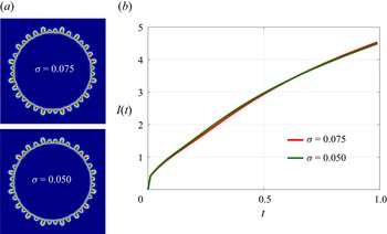
where we fix  $\sigma =0.075$ in all the simulations so that the exponential function introduced to deal with the singularity at the origin has no effect on the VF dynamics. We consider the fluid
 $A$ inside a circle of initial radius
 $r_0$ and
 $\sigma \leq r_0$ so that the exponential function has no effect on the VF dynamics. This is due to the fact that with an increase in
 $r$ (where
 $r^2=x^2+y^2)$, the exponential term will eventually decay and will have no effect on the velocity. We consider the computational domain
 $\varOmega =[-0.75,0.75] \times [-0.75,0.75]$ and we have taken
 $r_0=0.075$, so that the initial circular region has covered less than
 $1\,\%$ of the total computational domain. See Appendix A for the effect of different
 $\sigma$ on the dynamics. It must be noted that
 $\boldsymbol {u}_{pot}$ is the total velocity in the absence of any viscosity gradient but as soon as the reactants come in contact to generate a more viscous or less viscous product than the reactants, the viscosity gradient alters the total velocity. Thus, we consider the total velocity to contain two components
 \begin{equation} \boldsymbol{u}= \boldsymbol{u}_{pot}+\boldsymbol{u}_{rot}, \end{equation}
where  $\boldsymbol {u}_{rot}$ is the velocity component due to the chemical reaction and must be computed at each time, whereas
 $\boldsymbol {u}_{pot}$ is known at all time. To compute
 $\boldsymbol {u}_{rot}$, we use stream function
 $\psi$ defined as
 $\boldsymbol {u}_{rot}=({\partial \psi }/{\partial y}, -{\partial \psi }/{\partial x})$. We take curl of the Darcy's law (2.2b) to obtain stream function vorticity formulation
 $$\begin{gather} \nabla^2 \psi ={-}\omega, \end{gather}$$
 $$\begin{gather}\omega=R_c\left(v \frac{\partial c}{\partial x}-u \frac{\partial c}{\partial y}\right). \end{gather}$$
Here,  $\omega$ is the
 $\hat {\boldsymbol {k}}$ component of the vorticity vector. Equation (3.13) coupled with the convection diffusion equation (3.8) for
 $h$ is solved to explore the VF dynamics after using (3.9) to obtain the species concentration from
 $h$. The boundary conditions used are
 $$\begin{gather} \psi =0, \end{gather}$$
 $$\begin{gather}\boldsymbol{\nabla} h \boldsymbol{\cdot} \hat{\boldsymbol{n}}=0, \end{gather}$$
at  $x=\pm L/2$,
 $y=\pm L/2$. Here,
 $\hat {\boldsymbol {n}}$ is the unit outward normal. We perform numerical simulations by using a hybridisation of compact finite difference method and the pseudo-spectral method (Sharma et al. Reference Sharma, Pramanik, Chen and Mishra2019). We employ a sixth-order compact finite-difference method (Lele Reference Lele1992) along the
 $y$-direction and Fourier sine expansion in the
 $x$-direction to solve the Poisson equation (3.13). In order to solve the convection–diffusion equation for
 $h$, we use the method of lines. The spatial derivatives are discretised using compact finite difference of sixth order. The thus obtained semi-discretised system of ordinary differential equations is solved using a third-order Runge–Kutta method. The time steps are adaptive for Runge–Kutta method and satisfy the Courant–Friedrichs–Lewy (CFL) condition. More details about the numerical method can be found in Sharma et al. (Reference Sharma, Pramanik, Chen and Mishra2019) and the references therein. For completeness, we give a pseudo-code in Appendix D.
3.1. Order of convergence
We discuss here the order of convergence of the numerical method. The time step  $dt$ is chosen adaptively in order to satisfy the CFL condition. Thus, we perform the convergence analysis for spatial discretisation only. The numerical method is said to be convergent if there exist two non-zero constants
 $C$ and
 $p$ such that
 $\vert s_{N}-s_0 \vert \leq C \, dx^p$. Here,
 $s_{N}, s_0$ are the numerical and the exact solution, respectively,
 $p$ is the order of the convergence and
 $C$ is independent of
 ${dx}$, the spatial step size. In other words, a numerical method is said to be of order
 $p$ if the error in numerical solution is
 ${O}({dx}^p)=M \, dx^p$ (Burden, Faires & Burden Reference Burden, Faires and Burden2015).
To find the order of convergence, we perform simulations for four sets of grid points  $n_x=n_y$ keeping all other parameters the same. In addition, we know
 $n_x=n_y=N+1$, where
 $N$ is the number of sub-intervals. The spatial step sizes are defined as
 ${dx}={dy}=L/N$ where
 $L$ is the domain length. We choose the numerical solution corresponding to the maximum value of
 $N$, that is,
 $N=1024$ as the exact solution denoted as
 $s_0=s_{1024}$. The error corresponding to each
 $N$ is computed as
 $\epsilon _N(t) ={{\|s_N-s_0\|}/{\|s_0\|}}$. Further, we consider the worst-case scenario and denote the error for the solution with
 $N$ sub-intervals as
 $E_N ={\max _{0 \leq t \leq 1}\epsilon _N(t)}$. We compute the order
 $p$ of the numerical method as (Ding, Spelt & Shu Reference Ding, Spelt and Shu2007; Burden et al. Reference Burden, Faires and Burden2015; Jain, Mani & Moin Reference Jain, Mani and Moin2020)
 \begin{equation} p=\log_2 \left({\frac{E_{N}}{E_{2N}}}\right). \end{equation}
We follow the steps below to find order.
Step 1: Compute the numerical solution  $s_N$ for each
 $N$. We take
 $s_N, s_0$ as the concentration of reactants as well as product by replacing
 $s$ by
 $a, b, c$, respectively.
Step 2: The error  $\epsilon _N(t) ={{\|s_N(x,y)-s_0(x,y)\|}/{\|s_0(x,y)\|}}$ for various grid points is calculated. We denote the discretised
 $x$ and
 $y$ domain for
 $N=128$,
 $256$ and
 $512$ as
 \begin{equation} \left.\begin{array}{c@{}}
\boldsymbol{x}=\{x_0(={-}0.75), x_1, x_2 , \ldots, x_j
,\ldots x_N({=}0.75)\}, \\ \boldsymbol{y}=\{y_0(={-}0.75),
y_1, y_2 , \ldots, y_j ,\ldots y_N({=}0.75)\}.
\end{array}\right\} \end{equation}
In addition, the discretised  $x$ and
 $y$ domain for
 $N=1024$ is denoted as
 \begin{equation} \left.\begin{array}{c@{}}
\boldsymbol{X}=\{X_0(={-}0.75), X_1, X_2 , \ldots, X_j
,\ldots X_N({=}0.75)\}, \\ \boldsymbol{Y}=\{Y_0(={-}0.75),
Y_1, Y_2 , \ldots, Y_j ,\ldots Y_N({=}0.75)\}.
\end{array}\right\} \end{equation}
For any  $N$, we compute
 $\epsilon _N(t)$ as
 \begin{equation} \epsilon_{N}(t)= \frac{\|s_{N}(x=x_i,y=y_j)-s_0(x=X_{\varDelta i}, y=Y_{\varDelta j})\|}{\|s_0(x=X_{\varDelta i},y=Y_{\varDelta j})\|}, \end{equation}
where  $i=\{0,1,2, \ldots N\}$ and
 $j=\{0,1,2, \ldots N\}$ and
 $\varDelta =1024/N$. For example,
 $\epsilon _N(t)$ for
 $N=512$ is computed as
 \begin{equation} \epsilon_{512}(t)= \frac{\|s_{512}(x=x_i,y=y_j)-s_0(x=X_{2i}, y=Y_{2j})\|}{\|s_0(x=X_{2i},y=Y_{2j})\|}, \end{equation}
for  $i=\{0,1,2, \ldots 512\}$ and
 $j=\{0,1,2, \ldots 512\}$. Here we present results using 2-norm. However, it is verified that results are independent of the norm.
Step 3: Find the error as  $E_N ={\max _{0 \leq t \leq 1}\epsilon _N(t)}$.
Step 4: Compute order of convergence of the numerical method.
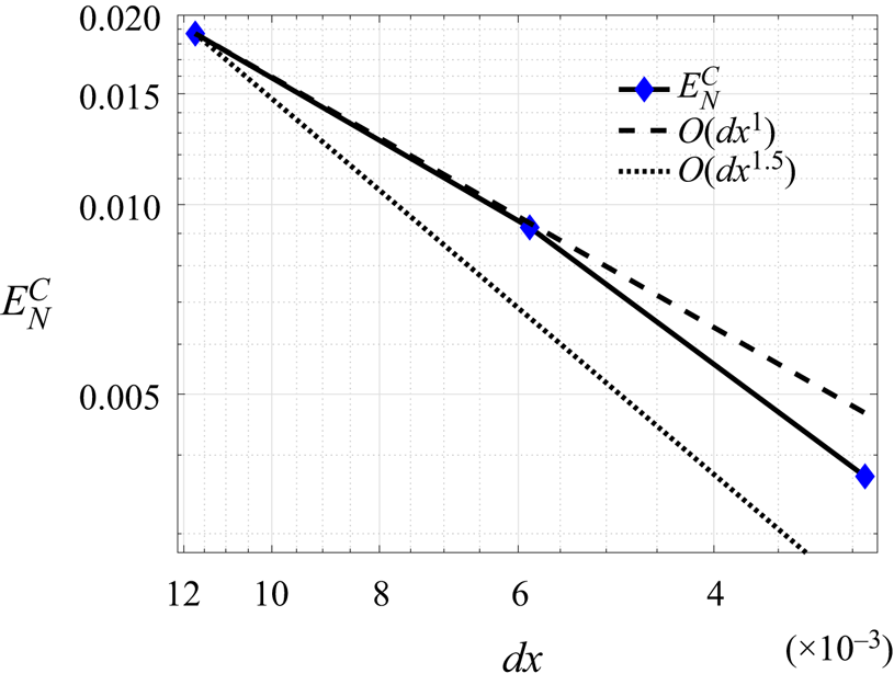
We present the error and the order in table 1. It is evident that with an increase in  $N$, the error reduces significantly. We plot the error in numerical solution of product concentration
 $E_N^C$ as a function of
 ${dx}$ in figure 2. In addition, reference lines with slope
 ${dx}, {dx}^{1.5}$ are plotted. It is evident that the order of convergence of the method lies between 1 and 1.5. There exist many studies (Ding et al. Reference Ding, Spelt and Shu2007; Sudarshan Kumar, Praveen & Veerappa Gowda Reference Sudarshan Kumar, Praveen and Veerappa Gowda2014; Liu & Ding Reference Liu and Ding2015; Jain et al. Reference Jain, Mani and Moin2020) where the order of convergence of the method is lower than the order of discretisation of the derivatives. In our work also, the spatial discretisation is performed using sixth order compact finite difference at the internal grid points, while the boundary points are discretised using third and fourth order compact finite difference. But since we have a coupled system of PDEs, we believe that order between 1 and 1.5 is adequate as evident from small error in table 1.
Error and order for various  $N$. Used parameters are
 $Pe=2000$ and
 $R_c=0$. Here,
 $E_N^C$,
 $E_N^A$ and
 $E_N^B$ denote the error in numerical solution of product concentration, reactant
 $A$ concentration and reactant
 $B$ concentration, respectively.

Error in product concentration  $E_N^C$ versus
 ${dx}$ for
 $Pe=2000$ and
 $R_c=0$. The dashed and dotted lines represent the reference lines with slope
 ${dx}$ and
 ${dx}^{1.5}$, respectively.

4. Results and discussion
VF induced by chemical reaction was discussed by Sharma et al. (Reference Sharma, Pramanik, Chen and Mishra2019) and it was observed that for a given finite reaction rate ( $Da$) and
 $Pe$, there always exists a range of
 $R_c$ for which only a stable displacement is observed. Motivated by this, we ask what happens if
 $Da \rightarrow \infty$, that is, the chemical reaction is instantaneous? For
 $Da \rightarrow \infty$, the reaction rate and, hence, the force due to reaction is strong enough to trigger any instability, but how the interplay of this force with forces due to convection and diffusion affect the overall VF dynamics is worth examining.
We consider reactants having no viscosity contrast and they undergo an infinitely fast chemical reaction upon contact, generating a product having the same or different viscosity. When all the species have the same viscosity, the product is generated in a ring between the reactants  ${A}$ and
 ${B}$ (see figure 1). Thus, the obtained region between
 ${A}$ and
 ${C}$ is regarded as the
 ${AC}$ front and that between
 ${B}$ and
 ${C}$ is regarded as the
 ${BC}$ front throughout this study independent of the displacement being stable or unstable. The product with different viscosity is of interest for us as the viscosity contrast results in the fingering instability due to the viscosity profile being a non-monotonic function of space. If the product is more viscous than the reactants, the viscosity profile experiences a maximum and, thus, the
 ${AC}$ front witnesses instability. On the other hand, for a less viscous product, a minimum is obtained in the viscosity profile, thereby making the
 ${BC}$ front unstable where a less viscous fluid displaces a more viscous fluid. We explore various features of VF due to a chemical reaction with an infinitely fast reaction rate between the reactants undergoing radial displacement.
4.1. Effect of different reactants on the VF dynamics
The outcome of a chemical reaction depends on the types of reactants considered. Hence, in this section, we discuss the VF dynamics by considering the reactants having different viscosity contrast and diffusion coefficients. Numerically,  $R_c$ and
 $Pe$ are the two parameters describing these properties. For a fixed
 $R_c$, a higher
 $Pe$ represents the reactants having a small diffusion coefficient and, hence, rigorous fingering instability is anticipated. Further, by the definition of
 $R_c$ in (2.5a,b), it is clear that
 $R_c>0$ corresponds to a more viscous product whereas a less viscous product is generated for
 $R_c<0$. We discuss the effect of these two parameters in order to understand the VF dynamics for a range of reactants undergoing infinitely fast chemical reaction.
4.1.1. Varying the viscosity of the reactants
As discussed,  $R_c>0$ corresponds to a more viscous product and, hence, the
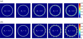
 ${AC}$ front is unstable to instability. In figure 3(a), product
 ${C}$ concentration for various
 $R_c>0$ is plotted (see Appendix E for components of velocity). We observe fingers towards the source (origin), in the form of a flower and the
 ${BC}$ front acts as a barrier to the instability preventing the fingers from penetrating further. Similarly for
 $R_c <0$, the fingers are observed at the
 ${BC}$ front away from the source and appear as a crown (see figure 3b). Further, with an increase in
 $\vert R_c \vert$, the fingering instability becomes more rigorous. These are in agreement with the existing numerical (Sharma et al. Reference Sharma, Pramanik, Chen and Mishra2019) and experimental (Nagatsu et al. Reference Nagatsu, Matsuda, Kato and Tada2007; Podgorski et al. Reference Podgorski, Sostarecz, Zorman and Belmonte2007) studies involving finite
 $Da$. Thus, these salient features of VF dynamics are independent of the reaction rate. The length of the fingers appear to depend on
 $R_c$ and we discuss this in detail in § 4.2.3. In addition, no deformations are observed for the displacement corresponding
 $\vert R_c \vert =1.5$ signifying completely stable displacement. Thus, despite an infinite
 $Da$, stable displacement is evident for some
 $\vert R_c \vert$ and fixed
 $Pe$.
Density plots of product  ${C}$ concentration at final time
 $t=1$ for
 $Pe=3000$ and (a)
 $R_c>0$ (in first row) (b)
 $R_c<0$ (in second row). Flower-like instability for
 $R_c \geq 2$ and crown-like instability for
 $R_c \leq -2$ is evident.

4.1.2. Effect of Péclet number
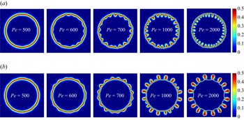
Fixing  $R_c$, we vary the Péclet number to explore the effect of diffusion on the fingering dynamics. We plot the density plots of the product concentration at non-dimensional final time
 $t=1$ for
 $R_c =5$ in figure 4(a) and
 $R_c=-5$ in figure 4(b). As the
 $Da$ is infinite, sufficient product is formed as soon as the reactants come in contact and, hence, rigorous instability is anticipated as convection is strong near the source. Indeed, with an increase in
 $Pe$, fingering instability is evident, however, stable displacement is observed for the smallest
 $Pe (=500)$ shown. Thus, despite the reaction rate being infinite and a high viscosity contrast (
 $\vert R_c\vert =5$ here), the diffusion is strong enough to prevent the instability. Thus, for a given viscosity contrast between the reactants, stable displacement is observed which is in agreement with the existing recent studies (Sharma et al. Reference Sharma, Pramanik, Chen and Mishra2019, Reference Sharma, Nand, Pramanik, Chen and Mishra2020) that reported an unfavourable viscosity contrast being insufficient to induce the instability when fluids undergo radial displacement. To the best of the authors’ knowledge, no stable displacement is reported when the reactants displace each other rectilinearly (Nagatsu & De Wit Reference Nagatsu and De Wit2011). Thus, three processes due to convection, diffusion and reaction interplay and affect the overall dynamics, and it can be concluded that a stable region including a range of
 $R_c$ for a fixed
 $Pe$ and
 $Da$ for which no VF is observed (Sharma et al. Reference Sharma, Pramanik, Chen and Mishra2019) never vanishes. We gain more insight into this by finding the onset time of instability in the next subsection.
Density plots of product  ${C}$ concentration for various
 $Pe$ and (a)
 $R_c=5$ (in first row) and (b)
 $R_c=-5$ (in second row) at final time
 $t=1$.

4.2. Unstable displacements
We have shown in the previous section that a stable displacement exists despite an infinite Damköhler number, but here we explore the unstable displacements. We start by understanding how the onset time varies with varying viscosity contrast and the Péclet number and then gain insight into the overall VF dynamics.
4.2.1. Onset of instability
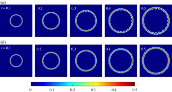
The time when the fingers start to appear is referred to as the onset time of instability denoted as  $t_{on}$. The density plots of product concentration for
 $\vert R_c\vert =4$ and
 $Pe=1000$ are shown in figure 5. It is evident from figure 5(a) that the fingering appears early for
 $R_c=4$ in comparison with
 $R_c=-4$ in figure 5(b). This is due to the
 ${AC}$ front where the radial velocity is higher (than at
 ${BC}$ front), is unstable for
 $R_c>0$. We quantify the onset time with the help of the interfacial length defined as (Sharma et al. Reference Sharma, Pramanik, Chen and Mishra2019)
 \begin{equation} I(t)=\int_{x_1}^{x_2}\int_{y_1}^{y_2} \sqrt{\left(\frac{\partial c}{\partial x}\right)^2+\left(\frac{\partial c}{\partial y}\right)^2}\, {{\rm d}y} \, {{\rm d}x}. \end{equation}
The product has the same viscosity as the reactants for  $R_c=0$ and, hence, a stable displacement is observed. We denote the interfacial length corresponding to
 $R_c=0$ as
 $I_0$ and use the same as the reference for stable displacement. If the interfacial length for any
 $R_c\neq 0$ coincides with
 $I_0$ for some time, we regard the displacement as stable up to that time and denote the time when the two interfacial length curves start to deviate as
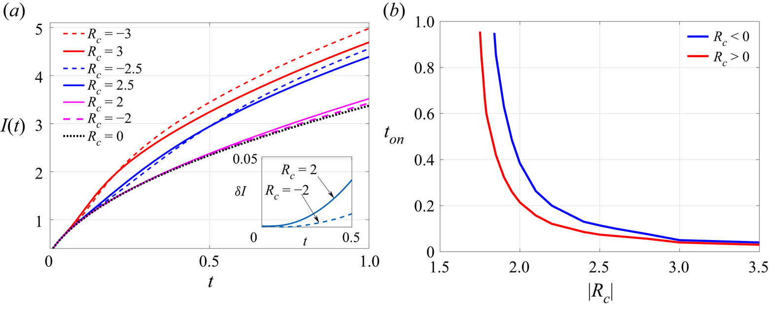
 $t_{on}$. We plot the interfacial length as a function of time for various
 $R_c$ and
 $Pe=3000$ in figure 6(a). Clearly, for some
 $\vert R_c \vert, I(t)$ for
 $R_c<0$ deviates from
 $I_0(t)$ at a later time in comparison with the deviation for
 $R_c>0$, indicating an early onset for
 $R_c >0$. This is in contradiction to the delayed onset for
 $R_c>0$ reported in the rectilinear geometry (Hejazi et al. Reference Hejazi, Trevelyan, Azaiez and De Wit2010). This can be attributed to the key difference between the rectilinear and the radial displacement which arises due to their respective velocity profiles. In rectilinear displacement, velocity profile is uniform (Tan & Homsy Reference Tan and Homsy1986) which results delayed onset for
 $R_c>0$ as instability appears in a direction opposite to the flow. However, in radial geometry, the velocity is spatially varying; the radial component of velocity being
 $u_r= 1/ 2 {\rm \pi}r$ (Tan & Homsy Reference Tan and Homsy1987). This velocity feeds instability with higher convective velocity when product is more viscous and instability appears at
 ${AC}$ front resulting in early instability for
 $R_c>0$. Further, it is observed that with an increase in
 $\vert R_c \vert$, the deviation occurs at the same time (see figure 6a) as sufficient product to trigger the instability is generated early. This is in agreement with the instability generated by a chemical reaction with finite
 $Da$ (Sharma et al. Reference Sharma, Pramanik, Chen and Mishra2019). Of course, for a fixed
 $Pe$ and
 $R_c$, the onset is early with an increase in
 $Da$ but the force due to convection is the ultimate force out of the three forces due to convection, diffusion and reaction in action, deciding onset in this case.
Temporal evolution of concentration of product for (a)  $R_c=4$ (in first row) and (b)
 $R_c=-4$ (in second row) for
 $Pe=1000$. The instability appears at
 $t\approx 0.2$ for
 $R_c =4$ while at
 $t \approx 0.3$ for
 $R_c=-4$.

(a) Temporal evolution of the interfacial length for various  $R_c$ and
 $Pe=3000$. Clearly, the onset of instability is early for
 $R_c>0$. Inset:
 $\delta I$ versus
 $t$ for
 $\vert R_c\vert =2$ showing the delayed onset for
 $R_c =-2$. (b) The onset time versus
 $\vert R_c\vert$ showing a delayed onset for
 $R_c<0$.

For a fixed  $Pe$, we calculate the absolute difference
 $\delta I(t)=\vert I(t)-I_0(t)\vert$ in the interfacial length of
 $R_c \neq 0$ and
 $R_c=0$ and define the onset time of instability as
 \begin{equation} t_{on}=\min \{ t>0: \delta I>tol \}, \end{equation}
where we have used  $tol$ to be
 $O(10^{-3})$. We plot
 $t_{on}$ versus
 $\vert R_c \vert$ for
 $Pe=3000$ in figure 6(b). Clearly, the onset is early for a larger viscosity contrast. It is evident that the displacement is more stable for
 $R_c<0$ as
 $t_{on}$ is more than that for the corresponding
 $R_c>0$. Further, with an increase in
 $\vert R_c \vert$, the two curves approach each other indicating the onset time becomes independent of the sign of
 $R_c$ which is a feature of radial displacement (Sharma et al. Reference Sharma, Pramanik, Chen and Mishra2019). In addition, no
 $t_{on}$ is obtained for various
 $\vert R_c\vert$, for instance,
 $\vert R_c \vert =1.5$. This is because a stable displacement is observed for such viscosity contrast indicating that the force due to reaction is not sufficient to trigger the instability. We conclude that for any time
 $t< t_{on}$, stable displacement is observed, whereas the VF instability is visible for
 $t \geq t_{on}.$ Thus, the onset time can be used to divide the
 $t$–
 $R_c$ phase space into two zones with region below the curve being stable and the region above the curve being the unstable zone. Hence, this
 $t$–
 $R_c$ phase space provides information about the completely stable displacements and the time when instability is observed for the first time, if the displacement is unstable.
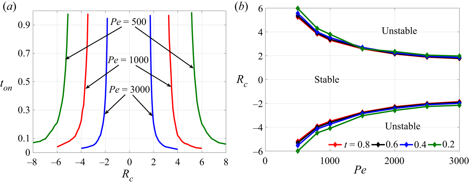
We determine the onset time of instability for various  $\vert R_c\vert$ by varying
 $Pe$. The onset time
 $t_{on}$ versus
 $\vert R_c \vert$ for various
 $Pe$ is shown in the figure 7(a). It is evident that for each
 $Pe$, the onset time follows the same trend as explained for
 $Pe=3000$. However, the stable zone in the
 $t$–
 $R_c$ phase space increases with a decrease in
 $Pe$. Interestingly, the onset time or, equivalently, the curves marking the boundary between stable and unstable region of
 $t$–
 $R_c$ phase space can be made independent of
 $Pe$ (see figure 9) using a rescaling which we obtain as explained in the following.
(a) Onset time  $t_{on}$ versus
 $R_c$ for
 $Pe=3000, 1000, 500$ showing a delayed onset for smaller
 $Pe$. (b) Plot for
 $R_c$ versus
 $Pe$ for a given time
 $t$.

4.2.2. Dependence of  $t_{on}$ on $R_c$ and $Pe$


As the width of the stable region is different for each  $Pe$, thus for each time, we find a relationship between the Péclet number and
 $R_c$. We explain in the following the procedure used to find a relation between
 $R_{c}>0$ and
 $Pe$. A similar procedure is used for
 $R_{c}<0$ and
 $Pe$. We fix a time
 $t$ and for a range of
 $Pe$, choose the
 $R_{c}>0$ values lying on the boundary between the stable and unstable zone of the
 $t$–
 $R_c$ phase space. Thus obtained
 $( Pe, R_{c})$ pairs are plotted for each
 $t$ as shown in figure 7(b). It is evident that for a fixed
 $Pe$, there exist a range of
 $R_c$ for which stable displacement is observed at the given time
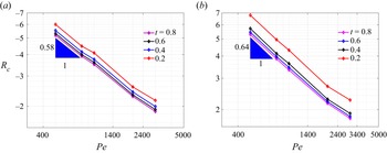
 $t$, indicating a continuous competition between the forces due to convection and diffusion. In fact, we find a stable zone sandwiched between two unstable zones for each time. Further, a log–log plot is given in figure 8. Interestingly, the curves thus obtained follow similar trend for each time
 $t$ and using the cftool of MATLAB (2020), we obtain a power law between
 $R_{c}^+$ and
 $Pe$ as
 \begin{equation} R_{c}^+= 260Pe^{{-}0.64}, \end{equation}
where  $R_c^+$ corresponds to the positive log-mobility ratio for which stable displacement is observed for all time and fixed
 $Pe$. Similarly, the power law obtained for the negative log-mobility ratio up to which flow is stable,
 $R_{c}^-$ and
 $Pe$ is
 \begin{equation} R_{c}^-= -160Pe^{{-}0.58}. \end{equation}
It is clear that the onset time will exist only when  $\vert R_c \vert > \vert R_c^\pm \vert$. Now, to obtain the dependence of the onset time on
 $R_c$ and
 $Pe$, we utilise the relation between
 $R_{c}^\pm$ and
 $Pe$. We assume a fitting for
 $t_{on}$ as
 \begin{equation} t_{on}\propto (\vert R_c\vert Pe^{\beta_1}-\beta_2)^{\beta_3}, \end{equation}
where the sign of  $R_c$ decides the constant of proportionality and
 $\beta _i$,
 $i=1,2,3$. The constants
 $\beta _1, \beta _2$ are obtained using (4.3), (4.4) and the fact that
 $t_{on}$ does not exist for completely stable displacement. Consequently, for any
 $R_c$ corresponding completely stable displacement,
 $t_{on}$ is not defined thus, we can take
 $$\begin{gather} \beta_1=0.64, \quad \beta_2=260 \quad \mbox{for}\ R_c>0, \end{gather}$$
 $$\begin{gather}\beta_1=0.58,\quad \beta_2=160 \quad \mbox{for}\ R_c<0, \end{gather}$$
and  $\beta _3$ must be negative. We obtain the constant of proportionality and
 $\beta _3$ using cftool of MATLAB (2020) and the onset time of instability for any
 $\vert R_c\vert$ and
 $Pe$ can be obtained as
 $$\begin{gather} t_{on}=31.1(Pe^{0.64}R_c-260)^{{-}1.22},\quad R_c>0, \end{gather}$$
 $$\begin{gather}t_{on}=437(Pe^{0.58}|R_c|-160)^{{-}1.85},\quad R_c<0. \end{gather}$$
Log–log plot of  $R_{c}$ versus
 $Pe$ at various times
 $t$. These curves can be well fitted using the power law
 $R_{c}^- = -160Pe^{-0.58}$ for
 $R_c<0$ in (a) and
 $R_{c}^+ = 260Pe^{-0.64}$ for
 $R_c>0$ in (b).

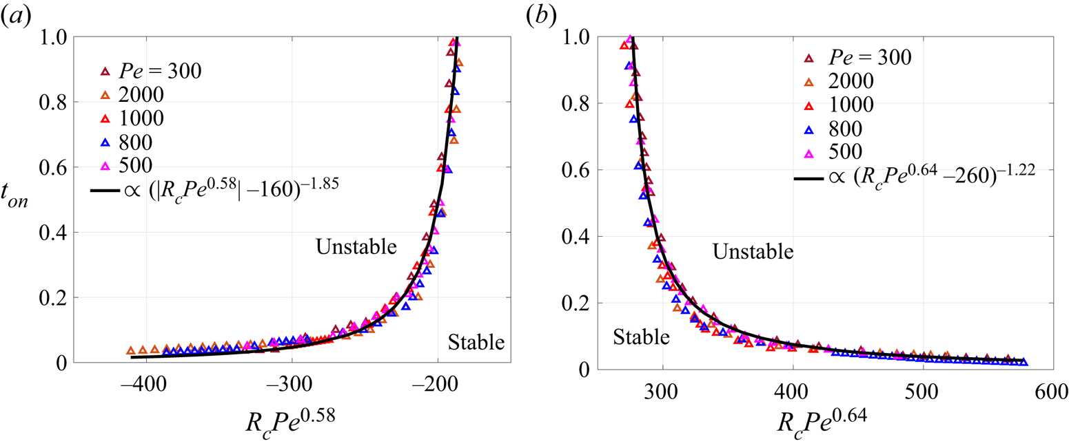
We plot  $t_{on}$ versus
 $R_c Pe^{\beta _1}$ for
 $R_c<0$ in figure 9(a) and
 $R_c>0$ in figure 9(b). The onset time appears independent of
 $Pe$ as all the points fall together around a single black curve which represents the onset time calculated in (4.8). In other words, the boundary between the stable and the unstable zone is found to follow the power law defined in (4.8). We obtain one boundary between the stable and unstable region independent of
 $Pe$. This relation can be used to find whether a displacement corresponding any
 $\vert R_c\vert$, and
 $Pe$ is completely stable or not. If
 $t_{on}$ is not defined which may happen when the quantity within the bracket in (4.8) is negative or zero, then the displacement is completely stable whereas a finite value of
 $t_{on}$ corresponds to the onset time for instability for the given
 $\vert R_c \vert$ and
 $Pe$.
Onset time curves for various  $Pe$, merged into a single curve for (a)
 $R_c<0$ and (b)
 $R_c>0$.

4.2.3. Finger length
After the onset of fingering instability, different dynamics are observed depending on  $Pe$ and the sign of
 $R_c$. In this section, we discuss these dynamics, focusing basically on the length of the fingers. Sharma et al. (Reference Sharma, Pramanik, Chen and Mishra2019) observed that for a fixed finite
 $Da$, the length of the fingers for
 $R_c>0$ is greater than that for corresponding
 $R_c<0$ but the two finger lengths approach each other with an increase in
 $Da$. However, for infinite
 $Da$, we observe that the length of the fingers depend upon
 $R_c$ and
 $Pe$ and a transition is observed which we discuss and quantify in the following.
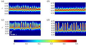
For better visualisation and comparison of the length of the fingers, we make the transformation from the  $(x,y)$ coordinates to
 $(r,\theta )$ coordinates as in (Sharma et al. Reference Sharma, Pramanik, Chen and Mishra2019). The density plots of the product concentration are shown in figure 10 for
 $Pe=1000$ and various
 $R_c$. It must be noted that the fingers for
 $R_c<0$ appear at
 ${BC}$ front but we have reversed the vertical axis (
 $r$-axis) in figure 10(b,d) so that the fingers face in one direction for both positive and negative
 $R_c$ and ease the visual comparison. Evidently, the length of the fingers is larger for
 $R_c=4$ than for
 $R_c=-4$ (as evident from comparison of figure 10a,b). However, if we compare the length for
 $\vert R_c \vert =5.5$ in figure 10(c,d), the trend seems to be opposite with the fingers being visibly longer for
 $R_c=-5.5$ than for
 $R_c=5.5$.
Density plots of product concentration in the  $(r,\theta )$ coordinates for
 $Pe=1000$ and (a)
 $R_c=4$, (b)
 $R_c=-4$, (c)
 $R_c=5.5$ and (d)
 $R_c=-5.5$ at final time
 $t=1$. For
 $R_c<0$, the vertical axis is reversed for a better comparison of the finger length.

In order to quantify the length of the fingers, we average the product concentration  $c(\theta,r,t)$ along the
 $\theta$ direction to obtain the averaged product concentration
 $\langle c(r) \rangle (t)$ as (Sharma et al. Reference Sharma, Pramanik, Chen and Mishra2019)
 \begin{equation} \langle c(r) \rangle (t) =\frac{1}{2 {\rm \pi}} \int_0^{2 {\rm \pi}} c(\theta,r,t)\, {\rm d}\theta. \end{equation}
The first and the last  $r$ values for which
 $\langle c(r) \rangle (t) > 0.005$ for
 $R_c=0$ are termed as
 $r_{0,in}$ and
 $r_{0,out}$ (Sharma et al. Reference Sharma, Pramanik, Chen and Mishra2019). Similarly,
 $r_{in}$ and
 $r_{out}$ are the points defined for
 $R_c \neq 0$. The distance between
 $r_{0,out}$ and
 $r_{out}$ denoted as
 $L_+$ corresponds to the length of the fingers at the
 ${BC}$ front. We refer to such fingers as outward fingers as these fingers appear away from the source. From the discussion so far, it is evident that the outward fingers are more prominent for
 $R_c<0$. Similarly the fingers at the
 ${AC}$ front are referred as the inward fingers with their length being denoted
 $L_-$ and being the distance between
 $r_{0,in}$ and
 $r_{in}$. Mathematically, we can write (Sharma et al. Reference Sharma, Pramanik, Chen and Mishra2019)
 \begin{equation} L_-=r_{0,in}-r_{in}, \quad L_+=r_{out}-r_{0,out}. \end{equation}
We plot the length of the fingers for a fixed  $Pe=1000$ and various
 $R_c$ in figure 11(a). Clearly, at all times,
 $L_-$ for
 $R_c=4$ is larger than
 $L_+$ for
 $R_c=-4$ which supports the observations of figure 10 and is a contradiction to the result in rectilinear geometry (Mishra, Martin & De Wit Reference Mishra, Martin and De Wit2008) where fingers are longer when the sample is less viscous. Further, with an increase in the magnitude of
 $R_c$, we observe a transition in the finger length with time. Initially, inward fingers are longer for
 $R_c=4.6$ than outward fingers for
 $R_c=-4.6$. After sometime, the outward fingers for
 $R_c=-4.6$ grow more than inward fingers for
 $R_c=4.6$. Ultimately, we observe a complete shift in the length of the fingers, the outward fingers are longer for
 $R_c=-5.5$ than the inward fingers for
 $R_c=5.5$ at all time except some initial time, as evident by a comparison of
 $L_+$ for
 $R_c=-5.5$ with
 $L_-$ for
 $R_c=5.5$. It is verified that
 $L_+$ for
 $R_c<0$ is longer than
 $L_-$ for
 $R_c>0$ on increasing
 $\vert R_c \vert$ further. Thus, fixing
 $Pe$, we observe that a transition in the length of the fingers is observed with an increase in
 $R_c$. Further, we see what happens if we vary
 $Pe$ for a fixed
 $R_c$ by plotting the finger length as a function of time in figure 11(b). It is evident that the trend in the relation between
 $L_+$ and
 $L_-$ reverses with an increase in
 $Pe$. Thus, we observe a unique dependence of the length of the fingers on the governing parameters which is not observed for finite
 $Da$ and appears to be a feature of an infinitely fast reaction rate. But what is responsible for this kind of dependence? To answer this question, we look back into the onset of instability and the spatially dependent velocity.
(a) Temporal evolution of  $L_-$ and
 $L_+$ for
 $Pe=1000$ and various
 $R_c$. (b) Length of inward and outward fingers for
 $R_c=5,-5$ and
 $Pe=2000, 700$. Here, solid lines are for
 $R_c=5$ and dashed lines are for
 $R_c=-5$. Clearly, transition in VF dynamics also occurs for a given viscosity ratio and varying
 $Pe$.

As discussed in § 4.2.1, the onset time of instability is early for  $R_c>0$ than for corresponding
 $R_c<0$ but the onset time becomes independent of the sign of
 $R_c$ with an increase in the viscosity contrast. This is due to the spatially varying velocity and is the reason behind the dependence of the length of fingers on
 $R_c$. As
 $t_{on}$ is early for
 $R_c=4$, so fingers start to grow at
 ${AC}$ front earlier and with faster convection velocity in comparison to the outward fingers for
 $R_c=-4$ which appear late and with lesser convection velocity. This results in larger
 $L_-$ for
 $R_c=4$ than
 $L_+$ for
 $R_c=-4$. As
 $\vert R_c \vert$ increases the difference between
 $t_{on}$ decreases and so do the finger length. Ultimately when
 $t_{on}$ is independent of the sign of
 $R_c$, the fingers appearing at the
 ${BC}$ front are longer than the inward fingers as the outward fingers grow radially outward in the direction of the flow which results in
 $L_+$ for
 $R_c<0$ to be more than the
 $L_-$ for the corresponding
 $R_c>0$.
5. Conclusion
The VF dynamics induced by an infinitely fast chemical reaction between reactants having the same viscosity and undergoing radial displacement has been discussed. The numerical complexity arises due to a non-dimensional number  $Da \rightarrow \infty$ for such chemical reactions. Thus, for the mathematical modelling of such reactions, the governing equations must be dealt with properly to achieve numerical convergence. We present the governing equations comprising a system of three coupled CDR equations each containing
 $Da$. However, it has been shown that using suitable transformation, the dynamics can be understood using only one convection–diffusion equation, coupled to the equations of fluid flow. The resulting system of equations is solved numerically using a hybrid numerical scheme based on compact finite difference and the pseudo-spectral method. The solution of the equations has been utilised to extract the knowledge about the concentration of the reactants as well as products, which has been used to see the relative effect of the forces due to convection, diffusion and reaction. We assume the reactants having the same viscosity and instability appears only when the product has different viscosity than the reactants. A more viscous product results in flower-like instability, whereas crown-like instability is observed when the product is less viscous than the reactants.
For  $Da \rightarrow \infty$, the chemical reaction results in a sufficient amount of product as soon as reactants come into contact and the displacement is expected to become unstable as soon as the product is generated. In contrast, we have observed stable displacement even for such high
 $Da$. Thus, an interplay of the forces due to convection, diffusion and reaction affects the overall dynamics. For
 $Da \rightarrow \infty$, although the force due to reaction is high but the triggering of the instability also depends upon other two non-dimensional parameters
 $Pe, R_c$ which are a measure of other two forces due to convection and diffusion. We quantify this by measuring the onset time of instability,
 $t_{on}$, which is the minimum time when the instability appears. Using density plots of the product concentration and quantification based on the interfacial length, it has been shown that the onset time of instability is a function of both
 $Pe$ and
 $R_c$. For a fixed
 $Pe$, the onset has been found to be delayed for
 $R_c <0$ which is in contrast to the results reported for rectilinear displacement (Hejazi et al. Reference Hejazi, Trevelyan, Azaiez and De Wit2010). However, the onset time becomes comparable for
 $\vert R_c \vert$ with an increase in the viscosity contrast between the reactants and the product, and this has been found to affect the fingering dynamics at a later time when finger length is found to depend on sign of
 $R_c$. On the other hand, the onset time increases with a decrease in
 $Pe$ for a fixed
 $R_c$, as the stabilising force due to diffusion is strong for smaller
 $Pe$. Using a proper fitting, we have made the onset time independent of
 $Pe$ and it has been observed that
 $t_{on}$ curves for various
 $Pe$ merge into a single curve. The onset time divides the entire time into two parts, one corresponding stable displacement when
 $t < t_{on}$, and unstable displacement is observed for the remaining time
 $t \geq t_{on}$. Thus, the onset time of instability divides the
 $t-R_c$ phase space into three zones with a stable zone sandwiched between two unstable zones. There exist reactions for which no finite
 $t_{on}$ is observed, a stable displacement at all times is observed for such reactions, which is never observed for rectilinear displacement.
Further, we have analysed the evolution of the fingering patterns at later times. For  $R_c<0$, the outward fingers appear while inward fingers are observed for
 $R_c>0$. It has been reported that the inward fingers for
 $R_c>0$ are longer than outward fingers for
 $R_c<0$, which is in contrast to that observed for rectilinear displacement (Mishra et al. Reference Mishra, Martin and De Wit2008). This is due to larger convection at unstable front and early onset time for
 $R_c>0$. However, with an increase in
 $\vert R_c \vert$, the inward finger length for
 $R_c>0$ and the outward finger length for
 $R_c<0$ approach each other and we observe a transition in the finger length. There exists a
 $\vert R_c \vert$ for fixed
 $Pe$ after which the outward finger length for
 $R_c<0$ becomes larger than the inward fingers for
 $R_c>0$. This transition appears to be due to infinite
 $Da$ as no such transition is reported for finite
 $Da$ (Sharma et al. Reference Sharma, Pramanik, Chen and Mishra2019). Similar transition in VF dynamics has been obtained for varying
 $Pe$ and a given viscosity ratio. In this work, we have considered the reactants having equal initial concentration, whereas exploring the dynamics when the initial concentration of reactants is not equal will be part of future work.
Our results help us to understand nonlinear interaction between chemical reaction and VF dynamics. The study finds application in controlling VF using chemical reaction, for increasing mixing in micro-fluidic devices and in point-of-care devices.
Acknowledgement
We are grateful to Professor C.-Y. Chen, National Yang Ming Chiao Tung University, Taiwan for fruitful discussions during preliminary stages of the work.
Funding
M.M. acknowledges financial support from SERB, Government of India, through project grant number CRG/2020/000613. P.V. acknowledges UGC, Government of India, for financial support through a PhD fellowship.
Declaration of interest
The authors report no conflict of interest.
Appendix A. Grid independence and effect of $\sigma$

We present here the convergence study for spatial discretisation. We did not perform any temporal convergence study as the time stepping is adaptive and is obtained using the CFL condition. The existing results in this article are for  $N=512$ in the
 $x$ as well as
 $y$ direction, where
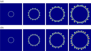
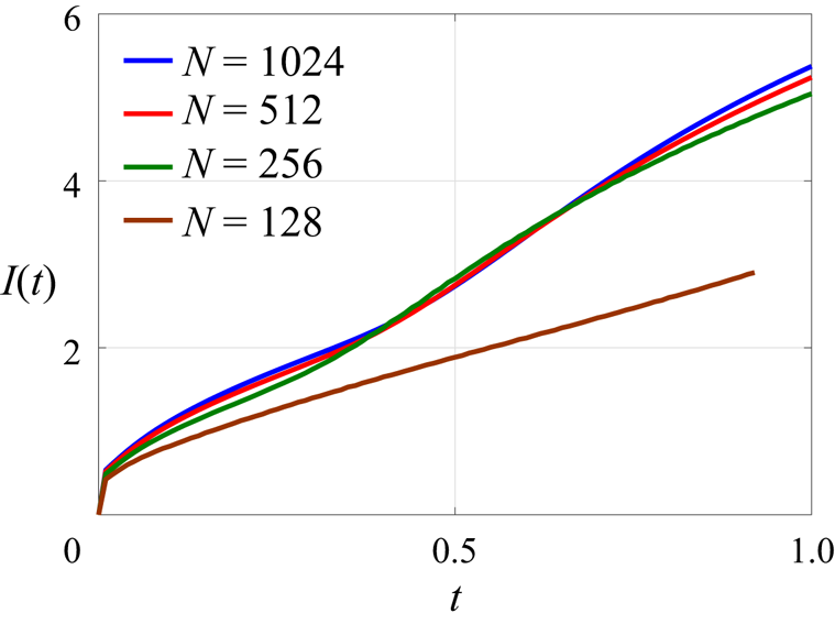
 $n_x=n_y=N+1$. We show that the results remain the same on taking double the grid points. We did not go for higher grid points as it increases the computational cost. The density plots of the product concentration are shown in figure 12 and the interfacial length is plotted in figure 13 for
 $R_c=-3.5,~ Pe=3000$. It can be observed that the grid independence is achieved for
 $N=512$.
Temporal evolution of concentration for  $R_c=-3.5$,
 $Pe=3000$ for (a)
 $N=512$ (in first row) and (b)
 $N=1024$ (in second row) at time
 $t=0.1$, 0.4, 0.7 and 1 (left to right).

Interfacial length for  $Pe=3000$,
 $R_c=-3.5$ for various grid points.

A.1. Effect of $\sigma$ on fingering dynamics

For a fixed  $r_0$, and
 $\sigma \leq r_0$, the VF dynamics are found to be identical as shown in figure 14. Both the fingering patterns as well as the interfacial length are the same for the different values of
 $\sigma$ considered.
(a) Product concentration profile at time  $t=1$ and (b) interfacial length for
 $Pe=3000$,
 $R_c=-2.5$,
 $r_0=0.075$ and various
 $\sigma$. Evidently, both concentration plot and interfacial length are identical for
 $\sigma \leq r_0$.

Appendix B. Why $h<0.5$ when $a=0$?


When the reaction rate is infinite, the reaction time tends to zero. As a result, the reactants are consumed immediately as soon as they come in contact. Thus, for  $t>0$, reactants does not co-exist in the entire domain of numerical experiment, except at the reaction front. Even at the reaction front, the reaction concentration reduces and
 $a \rightarrow 0$,
 $b \rightarrow 0$ and the maximum amount of product is generated. To gain more insight into this, we compute the angular averaged concentration
 $\langle s (r,t)\rangle$
 \begin{equation} \langle s(r,t)\rangle=\frac{\displaystyle \int_0^{2{\rm \pi}}s(r,\theta,t)\,{\rm d}\theta}{2{\rm \pi}}, \end{equation}
where  $s(r,\theta,t)$ is the concentration of
 $s$ in polar coordinates. Please note that
 $s$ is a dummy variable here. The averaged concentrations
 $\langle a(r,t)\rangle, \langle b(r,t)\rangle, \langle c(r,t)\rangle$ are calculated and plotted in figure 15 for
 $Da \rightarrow \infty$. The instantaneous reaction for
 $Da \rightarrow \infty$ results in the maximum expected amount of product at the reaction front as soon as the reactants come in contact. It is evident in figure 15 that the product concentration does not change much with an increase in time. However, the width of the Gaussian profile followed by
 $\langle c(r,t)\rangle$ increases with time on account of diffusion. The reactant concentration tends to zero at the reaction front and either one of the reactants is zero outside the reaction front, as shown in figure 15.
Temporal evolution of the angular averaged concentration plots of  $a, b, c$ for
 $Pe=3000$ and
 $Da \rightarrow \infty$.

To obtain  $a,b,c$ from
 $h$, we utilise the fact that the reaction occurs with an infinite reaction rate. The reaction front is the region where both the reactants co-exist and thus react to generate the product. However, as
 $Da\rightarrow \infty$, the two reactants are consumed as soon as they come into contact and, thus,
 $a, b$ tend to zero in the reaction front. Thus, from (3.5a,b) and the fact that
 $h_1=h=h_2$, we obtain
 \begin{equation} a+c=h=1-(b+c). \end{equation}
When  $a \rightarrow 0$, from the first pair, we obtain
 $h=c$. Using this and
 $b \rightarrow 0$ in the second pair
 $(h=1-(b+c))$, we obtain
 $h=0.5$. Hence, at the reaction front,
 $h=c=0.5$. The two reactants cannot co-exist outside the reaction front, that is, when
 $h\neq 0.5$. Thus, in the
 ${AC}$ zone, that is occupied by injected fluid reactant
 $A$ and the formed product
 $C$, we have
 $b=0$. Thus, from last pair, we obtain
 $c=1-h$. Substituting this is the first pair, we get
 $a+1-h=h \implies h=(1+a)/2$. In other words, we can say that
 $h>0.5$ in the
 $AC$ front. Similar logic holds for taking
 $h<0.5$ when
 $a=0$.
Appendix C. Different choices of $H_1, H_2$

In addition to that used in § 3, we can have two more choices of  $H_1$ and
 $H_2$ as
 \begin{equation} (H_1,H_2)=\{(a-b,a+c),(a-b,b+c)\}, \end{equation}
and obtain corresponding  $h_1, h_2$ using the normalisation in (3.2) as
 \begin{equation} (h_1,h_2)=\left\{ \left(\frac{a-b+1}{2},a+c\right), \left(\frac{a-b+1}{2},1-(b+c)\right)\right\}. \end{equation}
However, the dependence of  $a,b,c$ on
 $h$ remains the same as
 \begin{equation} (a,b,c)=\begin{cases} (0,1-2h,h) & h<0.5,\\ ({-}1+2h,0,1-h) & h \geq 0.5 \end{cases}. \end{equation}
Appendix D. Pseudo-code of the numerical method
Step 1: We consider a computational domain  $\varOmega =[-0.75,0.75] \times [-0.75,0.75]$ discretised into
 $n_x \times n_y$ grid points. At
 $t=0$, we give the initial condition for
 $h$. We consider the initial radius
 $r_0=0.075$ and utilise the axisymmetric base state solution of Tan & Homsy (Reference Tan and Homsy1987) at
 $t = r_0^2 /2$ as an initial condition for
 $h$. For velocity profile, we provide potential flow, i.e.
 $\boldsymbol {u}_{pot}$. We assign initial fluid concentrations as
 $a=h=1-b$ and
 $c=0$.
Step 2: The time is incremented by  $dt$ as
 $t \rightarrow t+d t$.
Step 3: The initial  $dt$ is
 $dt=10^{-6}$. Then we update
 $h$ value for time
 $t+d t$ by discretising the following convection diffusion equation:
 \begin{equation} \frac{\partial h}{\partial t}+\boldsymbol{u} \boldsymbol{\cdot} \boldsymbol{\nabla} h=\frac{1}{P e} \nabla^{2} h. \end{equation}
We descritise space derivative using a sixth-order compact finite-difference method and solve the resulting semi-discretised ordinary differential equation using a third-order Runge–Kutta method.
Step 4: After obtaining value for  $h$ at time
 $t+d t$, we assign fluid concentrations
 $a, b$ and
 $c$ as below
 \begin{equation} (a, b,
c)=\left\{\begin{array}{@{}ll} (0,1-2 h, h), & h<0.5
,\\ ({-}1+2 h, 0,1-h), & h \geq 0.5.
\end{array}\right. \end{equation}
Step 5: We use the updated value of  $c$ at time
 $t+d t$ to find the value
 $\omega$ as
 \begin{equation} \omega=R_{c}\left(v \frac{\partial c}{\partial x}-u \frac{\partial c}{\partial y}\right). \end{equation}
Step 6: Then we solve the Poisson equation  $\nabla ^{2} \psi =-\omega$ using a pseudo-spectral method. We employ a sixth-order compact finite-difference method along the
 $y$-direction and Fourier sine expansion in the
 $x$-direction.
Step 7: Time is again incremented by  $d t, t \rightarrow t+d t$. From this step,
 $dt$ is chosen adaptively by CFL condition.
Step 8: Steps 3–6 are repeated until the final time  $t_{f}$ or before the fluid reaches the boundary which is specified by checking if
 $h>0$ at 10 grid points away from the boundary,
 $x=\pm 0.75$,
 $y=\pm 0.75$ in the computational domain.
Appendix E. Pressure and velocity component
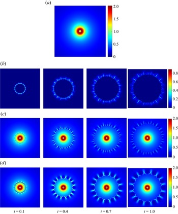
We plot  $\boldsymbol {u}_{pot}, \boldsymbol {u}_{rot}$ and the total velocity
 $\boldsymbol {u}$ in figure 16. As
 $\boldsymbol {u}_{pot}$ is independent of time and other parameters, it is shown only for one fixed time. It is evident that
 $\boldsymbol {u}_{pot}$ decreases with an increase in the distance from the origin. Further, because
 $\boldsymbol {u}_{rot}$ arises due to the viscosity contrast, it is non-zero only at the front where the product is generated or inside the fingers and is zero elsewhere. It decreases with time due to diffusion of the product with time. The total velocity
 $\boldsymbol {u}$ is obtained by adding the two components of velocity and it is evident from figure 16(c) and 16(d) that both components contribute to VF dynamics.
(a) Potential component of velocity,  $\boldsymbol {u}_{pot}$. Here, only one plot is shown as it does not depend on time,
 $Pe$ and
 $R_c$. Temporal evolution of (b) rotational component of velocity
 $\boldsymbol {u}_{rot}$ and (c) total velocity
 $\boldsymbol {u}=\boldsymbol {u}_{pot}+\boldsymbol {u}_{rot}$ for
 $R_c=-3.5$,
 $Pe=3000$. (d) Temporal evolution of total velocity
 $\boldsymbol {u}=\boldsymbol {u}_{pot}+\boldsymbol {u}_{rot}$ for
 $R_c=-5$,
 $Pe=2000$.

The pressure can be derived from Darcy's law as follows:
 $$\begin{gather} \boldsymbol{\nabla}p={-}\mu \boldsymbol{u}, \end{gather}$$
 $$\begin{gather}\Rightarrow \frac{\partial p}{\partial x}={-}\mu u, \quad \frac{\partial p}{\partial y}={-}\mu v, \end{gather}$$
 $$\begin{gather}\Rightarrow p={-}\int \mu u \, {{\rm d}x}+f(y), \end{gather}$$
 $$\begin{gather}\text{and} \quad-\mu v=\frac{\partial p}{\partial y}={-}\frac{\partial}{\partial y}\left(\int \mu u \,{{\rm d}x}\right) +\frac{\partial f}{\partial y}, \end{gather}$$
By the Leibnitz rule,
 $$\begin{gather} -\mu v={-\int \frac{\partial \mu}{\partial y} u-\mu \frac{\partial u}{\partial y } \,{{\rm d}x} +\frac{\partial f}{\partial y}}, \end{gather}$$
 $$\begin{gather}\Rightarrow \frac{\partial f}{\partial y}={-}\mu v+\int \frac{\partial \mu}{\partial y} u+\mu \frac{\partial u}{\partial y} \,{{\rm d}x}, \end{gather}$$
 $$\begin{gather}\Rightarrow f={-}\int \mu v \,{{\rm d}y}+ \int \left[\int \frac{\partial y}{\partial y} u+ \mu \frac{\partial u}{\partial y} \,{{\rm d}x}\right]\,{{\rm d}y} +c, \end{gather}$$
put  $f$ into (E1c)
 \begin{equation} \Rightarrow p={-}\int \mu u \,{{\rm d}x}-\int \mu v\, {{\rm d}y}+ \int\left[\int \frac{\partial \mu}{\partial y} u+\mu \frac{\partial u}{\partial y} \,{{\rm d}x} \right]\, {{\rm d}y} +c. \end{equation}