1. Introduction
The design of controls to delay transition from laminar to turbulent boundary-layer (BL) flow is a topic of fundamental engineering importance since it is directly related to the reduction of friction drag. For this reason, it has been one of the main subjects in fluid dynamics research for decades. The laminar–turbulent transition process in a BL can take different paths depending on the intensity of external disturbances (see e.g. Kachanov Reference Kachanov1994). For external disturbances with low intensity, the transition scenario starts with exponentially growing travelling waves which are commonly referred to as Tollmien–Schlichting (TS) waves (Tollmien Reference Tollmien1929; Schlichting Reference Schlichting1933; Schubauer & Skramstad Reference Schubauer and Skramstad1947). This linear instability is viscous, convective, and starts as the local flow Reynolds number exceeds a critical value. The TS waves grow in amplitude as they cross the unstable region of the BL while traveling in the downstream direction. When their amplitude reaches a critical value, which is of the order of 1 % of the free-stream velocity, TS waves undergo a secondary instability causing transition to turbulence (see e.g. Herbert Reference Herbert1988).
The stability properties can be significantly modified in a three-dimensional BL, compared with an ordinary two-dimensional BL, where spanwise variations of the streamwise velocity are introduced. Such spanwise modulations, commonly called streaks, are high- and low-speed regions elongated in the streamwise direction. Streaks can be generated for instance by free-stream turbulence, wall imperfections or in an artificial/controlled way and, depending on the characteristic spanwise wavelength, they can experience a large amplification in BLs. The underlying mechanism of streak generation and its amplification is described by the lift-up effect (see Landahl Reference Landahl1980), i.e. very weak streamwise vortices can generate important spanwise velocity modulations since they can lift up low-speed fluid from the region close to the wall into relatively faster flow and vice versa, exchanging momentum which, in turn, generates the streaks.
If the streak amplitude exceeds a threshold value (Andersson et al. Reference Andersson, Brandt, Bottaro and Henningson2001) it can lead to an inflectional instability of the BL (see e.g. Brandt & Henningson Reference Brandt and Henningson2002) bypassing the classical transition scenario related to the amplification of TS waves. Today it is, however, known that the BL is stabilized with respect to the growth of TS waves when streaks of moderate amplitude are present. The first observation of this stabilization was reported by Kachanov & Tararykin (Reference Kachanov and Tararykin1987), where steady streamwise streaks were generated in a controlled way by means of blowing through streamwise elongated slots in the plate. Later, unsteady streaks induced by free-stream turbulence were also observed to stabilize the growth of TS waves (Boiko et al. Reference Boiko, Westin, Klingmann, Kozlov and Alfredsson1994). However, in none of the above experimental works was transition delay reported. The stabilizing effect of the streaks is attributed to the extra turbulence production term, i.e. the streamwise–spanwise co-variance acting on the mean streamwise velocity gradient in the spanwise direction, which has been shown to be of negative sign and hence gives a stabilizing effect together with the viscous dissipation (Cossu & Brandt Reference Cossu and Brandt2004).
Several experimental studies have confirmed that streaks can delay the spatial growth of TS waves (Fransson et al. Reference Fransson, Brandt, Talamelli and Cossu2005) but also lead to transition delay in a low-noise environment (see e.g. Fransson et al. Reference Fransson, Talamelli, Brandt and Cossu2006; Sattarzadeh & Fransson Reference Sattarzadeh and Fransson2014; Shahinfar, Sattarzadeh & Fransson Reference Shahinfar, Sattarzadeh and Fransson2014). In addition, in the late stage of transition turbulent spots have been reported to spread much slower in the presence of unsteady streaks (Fransson Reference Fransson2010), which is believed to be caused by the same mechanism (i.e. the extra turbulence production term). Finally, in the above works it has been reported that the stabilizing effect of the streaks increases with their amplitude for a given spanwise wavelength. This means that in the use of streaks as a control strategy a dilemma appears. On the one hand a high amplitude is desired, since it enforces the stabilization, but on the other hand velocity streaks can undergo secondary instability if their amplitude exceeds a critical value (as discussed above), thus causing an advancement of the transition location, meaning that the control has failed.
In theoretical and numerical works optimal BL perturbations are often conveniently used in generating streamwise streaks (see e.g. Butler & Farrell Reference Butler and Farrell1992; Andersson et al. Reference Andersson, Brandt, Bottaro and Henningson2001). Optimal perturbations, i.e. perturbations which maximize their energy amplification as they propagate in the BL, consist of two counter-rotating streamwise vortices arranged in a periodic pattern in the spanwise direction with a spacing which is of the same order as the BL thickness. This kind of perturbation excites the lift-up effect and leads to the generation of streaks. Numerically, any type of initial condition can easily be implemented and then followed in time or space, which is not the case in an experiment. In fact, the global optimal perturbation has so far not been observed naturally nor has it been artificially generated, meaning that a detailed comparison with experiment is still lacking despite several attempts (see e.g. White Reference White2002; Fransson et al. Reference Fransson, Brandt, Talamelli and Cossu2004).
In real flows, streaks can be generated in several ways. Most commonly, experimental streaks are generated using surface-mounted devices which induce the lift-up effect. As discussed in White (Reference White2002), streaks generated by surface devices show some differences when compared with optimal perturbation theory. Typically, roughness elements of different shape are used to generate streaks, such as for instance circular cylinders (White Reference White2002; Konishi & Asai Reference Konishi and Asai2004; Fransson et al. Reference Fransson, Brandt, Talamelli and Cossu2005, Reference Fransson, Talamelli, Brandt and Cossu2006), bumps (see e.g. Piot, Casalis & Rist Reference Piot, Casalis and Rist2008) or sharp-edged rectangular roughness elements (see e.g. De Tullio et al. Reference De Tullio, Paredes, Sandham and Theofilis2013). In all cases, a horseshoe vortex forms at the base of each roughness element, which results in two streamwise counter-rotating vortices past the element. Generally, roughness elements also have a recirculating region and a wake whose stability properties can affect the stability of the BL. In particular, when circular roughness elements are used it is shown in Loiseau et al. (Reference Loiseau, Robinet, Cherubini and Leriche2014) that, if their dimensions exceed given threshold values, the wake past them becomes globally unstable and the interaction between the self-sustained wake instability and the BL can explain the earlier transition location which is observed experimentally (Fransson et al. Reference Fransson, Brandt, Talamelli and Cossu2005, Reference Fransson, Talamelli, Brandt and Cossu2006). This aspect limits the maximum amplitude of the streaks that can be generated, and thus their stabilizing capabilities.
Higher streak amplitudes can be obtained by employing small winglets, again mounted in a spanwise-oriented array, commonly referred to as miniature vortex generators (MVGs) (see e.g. Shahinfar et al. Reference Shahinfar, Sattarzadeh, Fransson and Talamelli2012). The small winglets constituting an MVG are arranged in pairs to generate counter-rotating vortices, which induce the lift-up effect leading to a streaky BL further downstream. Due to their aerodynamic shape, MVGs have smaller recirculating wakes than roughness elements and they can generate stable streaks which are significantly higher in amplitude than those produced by circular roughness elements. Moreover, regeneration of streaks is possible, thus extending the control effect in the streamwise direction (Sattarzadeh et al. Reference Sattarzadeh, Fransson, Talamelli and Fallenius2014).
Even though appealing alternative passive control strategies have recently been proposed for stabilizing TS waves (see e.g. Downs & Fransson Reference Downs and Fransson2014; Siconolfi, Camarri & Fransson Reference Siconolfi, Camarri and Fransson2015), at present MVGs are among the most widely investigated and promising devices for passive transition delay. Although MVGs have been extensively investigated and characterized, some aspects concerning their interaction with TS waves are still unclear and open. In particular, in all the documented experiments using MVGs in attenuating TS waves, the TS waves are generated upstream of the MVG array, so that the waves impinge on the array, with any subsequent complex interaction. This condition is more realistic and appropriate compared to the experiments in Fransson et al. (Reference Fransson, Brandt, Talamelli and Cossu2005, Reference Fransson, Talamelli, Brandt and Cossu2006), where the forced TS waves were generated downstream of the roughness elements.
In all the documented experiments the TS waves are always amplified in the near wake of the MVGs. Moving further downstream, a stable region is found where the TS waves are attenuated and the elongation of this region and the subsequent behaviour of TS waves depend on the configuration investigated. For some configurations (e.g. the MVG configurations C01 and C11 in Shahinfar et al. Reference Shahinfar, Fransson, Sattarzadeh and Talamelli2013) the stable region is long, even though the streak amplitude monotonically decays along the flat plate, and the TS waves are observed to monotonically damp as they move in the downstream direction for all the streamwise sections considered in the experiments. For other configurations (e.g. C09 and C05 in Shahinfar et al. Reference Shahinfar, Fransson, Sattarzadeh and Talamelli2013), after the first initial amplification which is common to all MVG configurations, the TS wave is attenuated, but further downstream a second instability region appears with both a branch I and a branch II. Thus, the TS wave experiences a second amplification before decaying monotonically further downstream. This particular behaviour, i.e. first the initial amplification behind the MVGs and secondly the appearance of a second unstable region further downstream, has not been investigated in detail previously and it is the subject of the present paper. It should be noted that the behaviour being addressed in the present study does not appear when the streaky base flow is generated by perturbations originating from optimal perturbation theory and simply plugged in to the base flow as an initial condition, as for instance in Cossu & Brandt (Reference Cossu and Brandt2002, Reference Cossu and Brandt2004).
The present paper is thus focused on explaining the experimental behaviour of TS waves when they are excited upstream of a MVG array. For this purpose, two representative cases among those reported in Shahinfar et al. (Reference Shahinfar, Fransson, Sattarzadeh and Talamelli2013) are considered, i.e. configurations C01 and C09, which are characterized by the two different behaviours of the TS waves mentioned above. In both cases small-amplitude TS waves are stabilized, thus they are appealing flow configurations for control purposes. In this paper the flow configurations C01 and C09 are simulated by direct numerical simulation (DNS) in the absence of incoming TS waves in order to obtain a detailed numerical flow field, which is validated against the available experimental data. The availability of DNS-like resolved flow fields for the configurations considered allows a detailed flow analysis, which would be very difficult and time consuming to obtain experimentally. Nevertheless, available experiments are used to validate the DNS results. In this paper, the DNS flow fields are investigated by local bi-global stability analysis so as to derive the stability curves for the controlled BL and to identify the unstable modes, when present. Moreover, the adopted numerical investigation allows the unstable modes of the controlled flow to be related to those of the uncontrolled one, providing new insight into the controlling effect of MVGs on TS waves.
Bi-global stability analysis generalizes the concept of local stability to three-dimensional flows which are weakly variable in one spatial direction (see Theofilis Reference Theofilis2003, for a review). In particular, for a developing BL which is mainly oriented along a streamwise direction as in the present case, a generic linearized disturbance is assumed to be homogeneous only in the streamwise direction, along which the true flow is slowly evolving, while it is supposed inhomogeneous in the remaining two directions. Thus, stability of the BL is investigated by solving a set of decoupled two-dimensional eigenvalue problems, one for each streamwise section considered. If the spatial stability is investigated, the eigenvalue problem is quadratically nonlinear, while it is linear for the temporal stability. In this paper the spatial stability of the controlled BL is investigated. Examples of applications of bi-global stability analysis to flows which are similar to the one considered here are, for instance, Riherd & Roy (Reference Riherd and Roy2013) for the flow past a plasma actuator inside a BL, Piot et al. (Reference Piot, Casalis and Rist2008) for the flow past a bump in a BL and De Tullio et al. (Reference De Tullio, Paredes, Sandham and Theofilis2013) for the flow past a rectangular-shaped roughness element in a supersonic BL. In the present paper the behaviour of the TS waves in the experiments is thus explained using the stability curves derived by applying stability analysis to the simulated flow fields. Moreover, the stability curves reported here are the first attempt to provide a complete and global picture of the stability properties of a BL controlled using MVGs.
2. Flow configurations and experimental setup
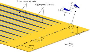
In this investigation we study the stability of streaky BLs developing over a flat plate under a zero pressure gradient in the streamwise direction. A representative sketch of the flow configuration considered in this paper is shown in figure 1 together with the frame of reference used in the following analysis. The coordinates
 $x,y$
and
 $z$
correspond to the streamwise, wall-normal and spanwise directions, respectively. The incoming free-stream velocity is
 $U_{\infty }$
. Two particular configurations are considered here, i.e. the cases C01 and C09 documented in Shahinfar et al. (Reference Shahinfar, Fransson, Sattarzadeh and Talamelli2013), whose characteristic parameters are summarized in table 1. The MVG arrays in the two configurations are located at
 $x=x_{\mathit{MVG}}$
from the leading edge. The two configurations differ only in the height,
 $h$
, of the MVGs (1.3 mm and 1.1 mm for C01 and C09, respectively) and in
 $U_{\infty }$
(
 $7.7~\text{m}~\text{s}^{-1}$
and
 $6.0~\text{m}~\text{s}^{-1}$
for C01 and C09, respectively). An MVG pair consists of two winglets mirrored in a streamwise centreline with an angle of
 $\pm 15^{\circ }$
as shown in the inset of figure 1. The spanwise wavelength between the MVG pairs is
 ${\it\Lambda}$
and the thickness of the winglets is equal to
 $t=0.3~\text{mm}$
. The two winglets constituting an MVG pair are separated by the distance
 $d$
at
 $L/2$
from the tip of the winglet where
 $L$
is the length of the winglet. Experiments have been carried out in air at atmospheric conditions with the kinematic viscosity
 ${\it\nu}=1.46\times 10^{-5}~\text{m}^{2}~\text{s}^{-1}$
. Defining the BL reference length as
 ${\it\delta}(x)=\sqrt{{\it\nu}x/U_{\infty }}$
, the ratio between the MVG height
 $h$
and
 ${\it\delta}$
at
 $x=x_{\mathit{MVG}}$
(see figure 1) is
 $h/{\it\delta}\simeq 2.0$
for C01 and
 $h/{\it\delta}\simeq 1.5$
for C09. Thus the height of the MVGs is equal to 0.40 and 0.35 times the total thickness of the BL
 ${\it\delta}_{99}$
in C01 and C09, respectively. The Reynolds number based on
 $U_{\infty }$
and the length scale
 ${\it\delta}$
is related to the Reynolds number based on the distance
 $x$
from the leading edge as follows:
 $Re_{{\it\delta}}=\sqrt{Re_{x}}$
.
Flow configuration sketch showing a flat plate with an MVG array generating low- and high-speed regions (i.e. streaks) inside the BL.

Geometrical and flow parameters for the C01 and C09 cases (Shahinfar et al. Reference Shahinfar, Fransson, Sattarzadeh and Talamelli2013).

In the experiments the TS waves were forced by means of periodic blowing and suction through a slot in a plug, which was flash mounted in the plate. The suction and blowing was accomplished using six sealed loudspeakers connected to the disturbance source slot via vinyl hoses. The loudspeakers were driven by a signal generator via three amplifiers, implying that the wave frequency (
 $f$
) was set when generating the signal and the forcing amplitude could be adjusted by the amplifiers. Here, we define the non-dimensional viscous frequency as
 $F=2{\rm\pi}f{\it\nu}\times 10^{6}/U_{\infty }^{2}$
. The measurements were performed using hot-wire anemometry and the TS wave amplitude was calculated based on the velocity signal filtered around the forcing frequency. For further details about the experimental setup the interested reader is referred to Shahinfar et al. (Reference Shahinfar, Fransson, Sattarzadeh and Talamelli2013).
3. Numerical tools
3.1. DNS
Besides the available experimental database, DNS have been carried out in order to have a detailed description of the velocity field past the MVGs. The simulations have been carried out using the code NEK5000 (http://nek5000.mcs.anl.gov/index.php/Main_Page), which is a massively parallel open-source flow solver based on a spectral-element method for incompressible flows. For each hexahedral spectral element of the spatial discretization, the basis functions are the Lagrangian interpolants based on the Gauss–Lobatto–Legendre quadrature points. The pressure field is numerically stabilized using basis functions of the order
 $N$
for the velocity and
 $N-2$
for the pressure. In the present work
 $N\geqslant 6$
. For the time discretization a third-order backward-difference scheme (BDF3) is used, with an explicit extrapolation for the nonlinear convective terms and an implicit treatment of the viscous terms.
Concerning the computational domain for the DNS (see figure 1), the periodicity of the MVG arrangement allows an extent in the spanwise direction equal to
 ${\it\Lambda}$
to be considered. The use of periodic boundary conditions in the spanwise direction including only one pair of MVGs, which thus might prevent the observation of sub-harmonic instabilities of the streaks in the DNS, is justified by the fact that the main objective of the present simulations is to compute the steady flow past the MVGs, whose stability properties are characterized here by a dedicated analysis. Moreover, experimental evidence shows that the streaks generated in the cases considered are stable in the absence of external excitation. A first campaign of DNS has been carried out using one single computational domain (D0) which includes the MVGs and extends in the streamwise direction from
 $Re_{x}\simeq 5.2\times 10^{4}$
to
 $Re_{x}\simeq 3\times 10^{5}$
. For comparison, the
 $Re_{x}$
location of the MVGs is reported as
 $Re_{x}^{\mathit{MVG}}$
in table 1 for the cases considered.
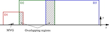
Results obtained with D0 are reported for the C01 case in Camarri, Fransson & Talamelli (Reference Camarri, Fransson, Talamelli, Talamelli, Oberlack and Peinke2013) and they have been used only for grid convergence studies, not shown here for the sake of brevity. As illustrated in Camarri et al. (Reference Camarri, Fransson, Talamelli, Talamelli, Oberlack and Peinke2013), it is necessary to consider a refined computational grid near each MVG to have a good evaluation of the flow past the vortex generator. This aspect might create a bottle-neck for the overall simulation, especially in terms of maximum time step for iterative stability. In order to overcome this problem, the steady flow is simulated using more overlapping domains, as sketched in figure 2. A first very refined domain, D1, includes only the MVG pair and the reduced size of the domain allows the use of three spectral elements in the thickness of each MVG winglet (recall that
 $t=0.3~\text{mm}$
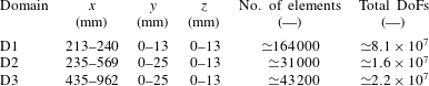
). The steady solution obtained in D1 is successively interpolated as a boundary condition for a partially overlapping domain D2, and the overlapping region is used to check the accuracy of the results and the quality of the overlapping between the results obtained in D1 and D2. A third domain, D3, has been used further downstream for C01, while this was not necessary for the C09 case as shown in the following. Details with respect to the domains D1, D2 and D3 are reported in table 2, and details on the validation of the method and on grid convergence for C01 can be found in Camarri et al. (Reference Camarri, Fransson, Talamelli, Talamelli, Oberlack and Peinke2013).
In the following section the boundary conditions (BCs) for the DNS are discussed. In domain D1 a fully developed Blasius BL is considered at the inflow and the no-slip condition is imposed at the solid walls. Periodic conditions are applied in the spanwise direction and, at the outlet and on the top boundary of the domain, free outflow boundary conditions are imposed as
 $\unicode[STIX]{x1D64F}\boldsymbol{\cdot }\boldsymbol{n}=\mathbf{0}$
, where
 $\unicode[STIX]{x1D64F}$
is the total stress tensor and
 $\boldsymbol{n}$
is the normal external vector of the computational domain boundary. For the D2 and D3 domains, the same BCs are used but an interpolated flow is imposed at the inflow, which is derived from DNS carried out on D1 and D2, respectively. This procedure to derive the inflow BCs has been validated for the same flow in Camarri et al. (Reference Camarri, Fransson, Talamelli, Talamelli, Oberlack and Peinke2013).
Sketch of the partially overlapping computational domains for the DNS.

Characteristics of the computational domains in the DNS (with reference to figure 2): dimensions in space, total number of elements and total degrees of freedom (DoF).

3.2. Stability analysis
The unsteady incompressible Navier–Stokes (NS) equations in their non-dimensional form can be written as follows:
 $$\begin{eqnarray}\displaystyle & \boldsymbol{{\rm\nabla}}\boldsymbol{\cdot }\boldsymbol{U}=0, & \displaystyle\end{eqnarray}$$
 $$\begin{eqnarray}\displaystyle & \displaystyle \frac{\partial \boldsymbol{U}}{\partial t}+\boldsymbol{U}\boldsymbol{\cdot }\boldsymbol{{\rm\nabla}}\boldsymbol{U}=-\boldsymbol{{\rm\nabla}}P+\displaystyle \frac{1}{Re}{\rm\nabla}^{2}\boldsymbol{U}, & \displaystyle\end{eqnarray}$$
 $\boldsymbol{U}(\boldsymbol{x},t)=(U,V,W)$
is the velocity vector,
 $P(\boldsymbol{x},t)$
is the reduced pressure and
 $Re$
is the Reynolds number. The flow field
 $(\boldsymbol{U},P)$
can be decomposed into a base flow
 $(\boldsymbol{U}_{0},P_{0})$
, i.e. the steady solution of the NS equations, and an unsteady perturbation field
 $(\boldsymbol{u},p)$
. In the bi-global stability analysis the base flow is considered weakly variable in the streamwise direction and perturbations are sought in the following modal form:
 $$\begin{eqnarray}\{u,v,w,p\}=\{\tilde{u} ,\tilde{v},\tilde{w},\tilde{p}\}(y,z)\text{e}^{\text{i}({\it\alpha}x-{\it\omega}t)},\end{eqnarray}$$
where i indicates the imaginary unit. Substituting the flow decomposition and the modal ansatz (3.3) into the NS equations, neglecting the higher-order terms of the perturbations and considering that the base flow is weakly variable in the streamwise direction, we obtain the following stability problem for each generic section in the streamwise direction:
 $$\begin{eqnarray}\displaystyle & \text{i}{\it\alpha}\tilde{u} +\displaystyle \frac{\partial \tilde{v}}{\partial y}+\frac{\partial \tilde{w}}{\partial z}=0, & \displaystyle\end{eqnarray}$$
 $$\begin{eqnarray}\displaystyle & -U_{0}{\it\alpha}\tilde{u} +{\it\xi}\tilde{u} +\text{i}\tilde{v}\displaystyle \frac{\partial U_{0}}{\partial y}+\text{i}\tilde{w}\frac{\partial U_{0}}{\partial z}-{\it\alpha}\tilde{p}+{\it\alpha}^{2}\frac{\text{i}}{Re}\tilde{u} =-{\it\omega}\tilde{u} , & \displaystyle\end{eqnarray}$$
 $$\begin{eqnarray}\displaystyle & -U_{0}{\it\alpha}\tilde{v}+{\it\xi}\tilde{v}+\text{i}\tilde{v}\displaystyle \frac{\partial V_{0}}{\partial y}+\text{i}\tilde{w}\frac{\partial V_{0}}{\partial z}+\text{i}\frac{\partial \tilde{p}}{\partial y}+{\it\alpha}^{2}\frac{\text{i}}{Re}\tilde{v}=-{\it\omega}\tilde{v}, & \displaystyle\end{eqnarray}$$
 $$\begin{eqnarray}\displaystyle & -U_{0}{\it\alpha}\tilde{w}+{\it\xi}\tilde{w}+\text{i}\tilde{v}\displaystyle \frac{\partial W_{0}}{\partial y}+\text{i}\tilde{w}\frac{\partial W_{0}}{\partial z}+\text{i}\frac{\partial \tilde{p}}{\partial z}+{\it\alpha}^{2}\frac{\text{i}}{Re}\tilde{w}=-{\it\omega}\tilde{w}, & \displaystyle\end{eqnarray}$$
 $$\begin{eqnarray}{\it\xi}=\left[\text{i}V_{0}\frac{\partial }{\partial y}+\text{i}W_{0}\frac{\partial }{\partial z}-\frac{\text{i}}{Re}\left(\frac{\partial ^{2}}{\partial y^{2}}+\frac{\partial ^{2}}{\partial z^{2}}\right)\right].\end{eqnarray}$$
The stability problem is completed by periodic boundary conditions in the spanwise direction and homogeneous Dirichlet conditions for the velocity field on the other boundaries. The system of equations (3.4) has been discretized in space at each streamwise section using a finite-element formulation with Taylor–Hood elements. The discretization has been carried out using the open-source program FreeFem++ (http://www.freefem.org). Once discretized, the stability problem (3.4) can be put into the form
 $(A_{0}+{\it\alpha}A_{1}+{\it\alpha}^{2}A_{2})\boldsymbol{q}={\it\omega}B\boldsymbol{q}$
, where the eigenvector is
 $\boldsymbol{q}=\{\tilde{u} ,\tilde{v},\tilde{w},\tilde{p}\}$
. For a temporal analysis
 ${\it\alpha}\in \mathbb{R}$
e is assigned and
 ${\it\omega}\in \mathbb{C}$
is the unknown eigenvalue of the analysis. In the spatial analysis the frequency
 ${\it\omega}\in \mathbb{R}$
e is given and
 ${\it\alpha}\in \mathbb{C}$
is the unknown eigenvalue. While the temporal analysis is a linear problem, the spatial analysis is a generalized quadratically nonlinear eigenvalue problem in
 ${\it\alpha}$
. In this paper the stability of the controlled BL has been characterized by a spatial stability analysis. The initial guess for the solution of the resulting nonlinear eigenvalue problem has been estimated by performing a temporal stability analysis and applying the Gaster transformation (see Gaster Reference Gaster1962) to the results. Both the linear and nonlinear eigenvalue problems have been solved by a Krylov–Schur method with a shift-invert technique, using the parallel implementation available in the SLEPc library (see Hernandez, Roman & Vidal Reference Hernandez, Roman and Vidal2005).
4. Numerical results
4.1. Base flow characterization near the MVGs
In this section the velocity and the vorticity fields for the flow in the proximity of a pair of MVGs are discussed so as to characterize the flow in the controlled BL. The objective is to show the aerodynamic behaviour of MVGs by providing details that would be difficult to measure experimentally because of their reduced characteristic lengths. Although the following discussion is focused only on case C09, it applies for case C01 as well because the flow details near the MVGs are very similar for the two cases.
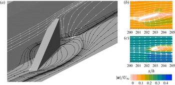
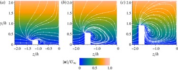
In figure 3(a) streamlines of the flow field, which is steady, are plotted for the case C09 on two selected planes so as to highlight the region of reversed flow. The local Reynolds number of the incoming flow, when scaled with the height of the MVG and the velocity external to the BL is low (
 $Re_{h}\simeq 456$
) and the MVG is completely immersed in the BL (recall that
 $h/{\it\delta}\simeq 1.5$
and 2.0 for the C09 and C01 cases, respectively). As a result, figure 3(a) shows that the flow around the MVG is quite regular and, despite its thickness, the recirculating regions are small. The topology of the streamlines on the plane where the MVG is installed indicates the presence of a saddle point at a distance beyond the MVG approximately equal to
 $h$
.
The streamlines in the vertical plane coming from the saddle point indicate that the size of the recirculating region quickly reduces with the distance from the plate. Laterally, on the side internal to the MVG pair, the flow is not recirculating. Note that the side of the MVG which is shown here is the most critical one for separation due to the incidence angle between the MVG and the incoming flow. Thus, recirculation is confined in a small region beyond the MVG. This is confirmed by figure 3(b,c), where streamlines and the velocity intensity are shown at two sections, namely
 $y/h=0.25$
and
 $y/h=0.75$
.
Streamlines near one MVG for case C09. (a) On two selected orthogonal planes (the black and the white streamlines are located on the wall and on the vertical plane respectively). Streamlines and contours of the velocity magnitude on horizontal sections at (b)
 $y/h=0.25$
and (c)
 $y/h=0.75$
.

Cross-sectional contours of velocity magnitude with the in-plane streamlines for the C09 case in the region near the MVG: (a)
 ${\it\chi}=0.21$
, (b)
 ${\it\chi}=0.55$
, (c)
 ${\it\chi}=0.90$
.

Although recirculations are very small, flow separation is expected on the face of the MVG considered. This takes place from the free edge and generates a streamwise vortex which induces the lift-up mechanism further downstream. In order to characterize the separation region, figure 4 show the on-plane streamlines and velocity intensity at three
 $x$
-sections from the MVG leading edge, namely
 ${\it\chi}=0.21$
,
 ${\it\chi}=0.55$
and
 ${\it\chi}=0.90$
, where
 ${\it\chi}=(x-x_{LE})/L$
. This figure confirms that flow separation occurs on almost the whole surface of the MVG internal to the MVG pair, the streamlines being spiral in shape and reattaching very close to the corner between the MVG and the flat plate. The main velocity component in this region is the one in the streamwise direction, the maximum on-plane velocity being approximately equal to
 $0.1U_{\infty }$
, and regions of reversed flow are absent. The core of the generated streamwise vortex is closed to the free edge of the MVG and it forms only on one side of the MVG. This observation indicates that the streamwise vortex is generated by the flow detaching from the free edge and it is not a horseshoe vortex which originates at its base, as occurs for roughness elements (see e.g. Loiseau et al.
Reference Loiseau, Robinet, Cherubini and Leriche2014). Thus, each MVG behaves similarly to an aerodynamic body and, in particular, to a delta wing. These flow features distinguish MVGs from wall-mounted roughness elements, typically characterized by an intense horseshoe vortex and by large regions of reversed flow in the wake, whose extent and stability depend on the local flow
 $Re$
and on the ratio between the height of the roughness and the local thickness of the BL. This aspect has been shown in Loiseau et al. (Reference Loiseau, Robinet, Cherubini and Leriche2014) to play an important role in the by-pass transition of the BL since large recirculations past roughness elements can become globally unstable, thus promoting the BL transition to turbulence. DNS, which is evolved in time until steady state is reached, have not shown the presence of any global instability in the wake past the MVGs. Although a rigorous global stability analysis would be necessary to definitely exclude the presence of a wake self-sustained instability, the stability of the wake suggested by DNS is compatible with the reduced size of recirculations observed and illustrated above and with the experimental evidence showing that the devices considered lead to a transition delay in the BL.
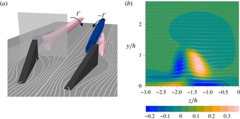
As highlighted above, from each MVG a strong streamwise vortex is generated, as shown in figure 5(a) which depicts this vortical system for the C09 configuration, where the streamwise vortices are identified by the
 ${\it\lambda}_{2}$
criterion (see Jeong & Hussain Reference Jeong and Hussain1995). A counter-rotating and equal vortex is generated by symmetry by the other MVG of a given pair. As can be evinced by figure 5(a), the velocity induced by this pair of vortices tends to push high-momentum fluid from the centreline of the MVG pair towards the wall and low-momentum fluid from the sides of the MVG pair toward the external part of the BL, giving rise to the lift-up mechanism. Since in the configurations considered the spacing between contiguous pairs is larger than the distance between the two MVGs of a single pair, the main effect of the MVGs is to generate high-speed streaks aligned with the symmetry line of each generating couple. The evolution of the streaks generated in this way is studied in detail in § 4.2 and compared with the experimental data.
Figure 5(a) shows that past a single MVG another vortex, counter-rotating with respect to the main one, is formed. This vortex is very weak and it is immersed inside a region with a large shear and axial vorticity that bounds the wake of the MVG, as shown in figure 5(b), where the streamwise vorticity is reported together with the in-plane velocity vectors in a
 $y$
–
 $z$
section at
 ${\it\chi}=1.25$
. The weak vortex vanishes at a very short distance past the MVG while the strong one persists for a large distance. In this respect we refer to Siconolfi et al. (Reference Siconolfi, Camarri and Fransson2015) where the intensity of the main vortex generated by each MVG in the configuration C01 is reported as a function of the streamwise coordinate.
(a) Representative isosurfaces of
 ${\it\lambda}_{2}$
for the C09 case in the region immediately downstream of the MVGs. The grey plane indicates the streamwise position of the section shown in (b). (b) Cross-sectional contours of streamwise vorticity together with the in-plane velocity vectors for case C09 at
 ${\it\chi}=1.25$
.

4.2. Streak evolution and validation against experiment
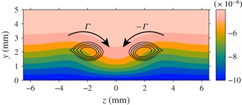
In this section the evolution of streaks obtained by DNS is analysed and compared with the available experimental measurements. As discussed in detail in § 4.1 each pair of MVGs generates two counter-rotating streamwise vortices which activate the lift-up mechanism leading to the formation of the velocity streaks in the BL. An example of this mechanism is shown in figure 6 where the streamwise velocity at a representative
 $x$
-section is plotted together with the identified streamwise vortices. The figure clearly shows that the streamwise vortices generated by each MVG pair induce a velocity field which pushes high-momentum fluid from the external region of the BL towards the wall, thus generating a high-speed streak. At the same time, but with a lower intensity due to the distance between contiguous MVG pairs, streamwise vortices elevate low-velocity fluid from the wall, generating small low-speed streaks with respect to the larger high-speed streak on the MVG centreline. Globally, figure 6 shows the base flow modulations induced by the MVGs, which are repeated periodically in the spanwise direction.
Contours of streamwise velocity field for the C01 case at the streamwise section where the streak amplitude is maximum. The solid black lines represent the two streamwise vortices identified by the
 ${\it\lambda}_{2}$
criterion and the two curved arrows depict the rotational direction of the vortices.

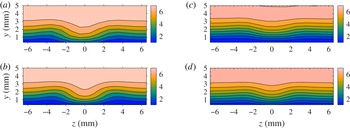
Contour plots of the streamwise velocity component for both C01 and C09 from experiments (a,c) and DNS (b,d). (a,b) The C01 case
 $x=381~\text{mm}$
(i.e.
 $Re_{x}\approx 1.96\times 10^{5}$
); (c,d) the C09 case
 $x=343~\text{mm}$
(i.e.
 $Re_{x}\approx 1.37\times 10^{5}$
).

A qualitative comparison between experiments and simulations can be carried out by looking at figure 7 where both DNS and experimental velocity fields are reported at streamwise sections near the point of maximum streak amplitude, which is approximately located at a distance equal to
 $122h$
and
 $110h$
past the MVGs for cases C01 and C09, respectively. These distances clarify the scale separation problem that exists between the flow near the MVGs, whose characteristic size is equal to
 $h$
, and the velocity modulations past the MVGs, which are slowly evolving in the streamwise direction. Figure 7 shows that the heights and shape of the simulated velocity modulations are in good qualitative agreement with the experiments at the distance past the MVGs considered.
In order to carry out a quantitative comparison and to investigate the streamwise evolution of the velocity streaks, it is convenient to adopt a definition of the streaky BL amplitude. A commonly used definition in the past was to consider the maximum base flow variation for each
 $x$
-position, normalized with
 $U_{\infty }$
. However, a local definition is not well-suited for experiments since it may be sensitive to the spatial resolution of the experimental measurements. In addition a local definition cannot be correlated with the stabilizing effect since it does not carry any information about the spanwise wavelength. For this reason, an integral measure is preferable and we here use the same definition as in Shahinfar et al. (Reference Shahinfar, Fransson, Sattarzadeh and Talamelli2013), namely
 $$\begin{eqnarray}A_{\mathit{ST}}^{\mathit{int}}(x)={\displaystyle \frac{1}{U_{\infty }}}\int _{-1/2}^{1/2}\int _{0}^{{\it\eta}^{\ast }}|U(x,y,z)-U^{z}(x,y)|\,\text{d}{\it\eta}\,\text{d}{\it\zeta},\end{eqnarray}$$
where
 ${\it\eta}=y/{\it\delta}(x)$
and
 ${\it\zeta}=z/{\it\Lambda}$
. The height of integration
 ${\it\eta}^{\ast }$
must be sufficiently large in order to obtain a result that is independent of its value. In this study we have chosen
 ${\it\eta}^{\ast }=9$
. The streamwise evolution of
 $A_{\mathit{ST}}^{\mathit{int}}$
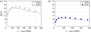
is reported for experiments and DNS in figure 8 for both C01 and C09, showing a substantial agreement between experiments (EXP) and DNS, with a maximum relative error of 4 % in
 $A_{\mathit{ST}}^{\mathit{int}}$
. As shown in figure 8 the vortices generated by the MVGs induce the formation of the velocity streaks, which form and undergo a transient growth in amplitude when moving in the downstream direction. Since the vortices are immersed in the BL, they are significantly damped by viscous effects as they are convected downstream, as quantified for C01 in Siconolfi et al. (Reference Siconolfi, Camarri and Fransson2015). At the same time nonlinear effects play a role in the saturation of the streak amplitude, as shown in Zuccher, Bottaro & Luchini (Reference Zuccher, Bottaro and Luchini2006). As a global effect, streaks initially grow rapidly due to the energetic consequences of the lift-up mechanism and to the similarity between the wake past the MVGs and the sub-optimal disturbances, and they reach the maximum value of
 $A_{\mathit{ST}}^{\mathit{int}}$
at distances of the order of
 $100h$
past the MVGs. Further downstream the streaks decay at a rate which is small compared to that of their initial growth.
Comparison between DNS and experimental results of the integrated streak amplitude evolution: (a) case C01 and (b) case C09.

Although the integral parameter
 $A_{\mathit{ST}}^{\mathit{int}}$
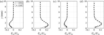
indicates a good agreement between experiments and simulations, a more detailed comparison is carried out in figure 9, where profiles of the streamwise velocity deviation from the averaged spanwise velocity profile at the centres of a high- and a low-speed streak are reported for the streamwise section where the maximum streak amplitude is measured experimentally, i.e. the fifth experimental point from left in figure 8. Figure 9 shows a fairly good agreement between experiments and DNS, with pointwise discrepancies in the velocity profiles in agreement with the error observed for the integral measure
 $A_{\mathit{ST}}^{\mathit{int}}$
.
Comparison between DNS and experimental profiles of the normalized streamwise velocity deviation
 $U_{p}$
from the averaged spanwise velocity
 $U^{z}$
(
 $U_{p}=U-U^{z}$
) at the location of a low-speed (a,c) and a high-speed (b,d) streak, at the streamwise station where the maximum streak amplitude is experimentally observed. (a,b) Case C01 and (c,d) case C09.

Several factors can cause the slight discrepancies between experiments and simulations highlighted above, although the agreement between the two is more than satisfactory for the purposes of the present work, especially considering the technical complexity of the experiments due to the geometric tolerances of the setup, the control of the flow quality in the wind tunnel and the difficulties in performing the velocity measurements.
4.3. Stability properties of the controlled boundary layer
4.3.1. Linear stability analysis of the DNS velocity fields
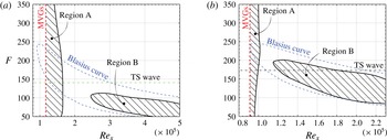
In this section a local spatial stability analysis is carried out of the flow fields obtained by DNS for cases C01 and C09 following the procedure described in § 3.2. The analysis is carried out by considering several sections in the streamwise direction, and the results are collected in the form of stability diagrams in the
 $F{-}Re_{x}$
plane (see figure 10
a,b). Both the C01 and the C09 cases are characterized by an unstable region, region A, located in the near-wake of the MVGs, which spans a large range of frequencies and ends at a given distance beyond the MVGs, where the flow becomes locally convectively stable. Comparing figure 10 with figure 8 it is possible to deduce that the unstable region A ends around
 $1.6\times 10^{5}$
for C01 and at around
 $1.1\times 10^{5}$
for C09 corresponding to
 $x-x_{\mathit{MVG}}\approx 90$
and 53 mm in figure 8, respectively, i.e. before the streak amplitudes have reached their corresponding maxima. Further downstream, the streaks start to decay and a second region of instability is identified, region B, whose shape resembles that of the uncontrolled Blasius BL, reported with a dashed line in figure 10 for comparison.
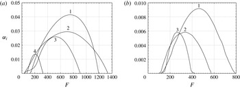
Region A is directly connected with the disturbance generated by the MVGs in the flow, and it starts just past the MVGs. In this region up to three (case C09) and four (case C01) unstable modes are identified, covering a large range of temporal frequencies. This is shown in figures 11(a) and 11(b), which report the results of the local spatial stability analysis carried out in a section lying inside region A for C01 and C09, respectively. As discussed in Piot et al. (Reference Piot, Casalis and Rist2008) and here in § 4.4, besides the identified unstable modes, the MVGs also excite stable modes, since they are an abrupt geometric discontinuity for the flow. Stable modes are successively damped in space, while unstable modes are damped only outside region A.
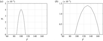
In region B, which is located further downstream past a region of stability for the BL, only one unstable mode is identified with a range of unstable frequencies comparable with that of the uncontrolled BL. This second region of instability originates since the streaks lose their intensity in the streamwise direction and, consequently, their control effect on TS waves weakens as the streak amplitude decreases. An example of typical stability results in region B is shown in figure 12(a,b) for the C01 and the C09 cases. Comparison between figures 11 and 12 can be misleading because they report local quantities, and the scenario can change with the streamwise sections considered. Nevertheless, local stability analysis generally predicts maximum spatial growth rates that can be significantly larger in region A if compared to region B, as for the case in figures 11 and 12. However, the maximum growth factors in the two regions are predicted at significantly different temporal frequencies, and unstable modes in region A are found at definitely higher frequencies than in region B.
Stability diagrams for cases C01 (a) and C09 (b) in the
 $F{-}Re_{x}$
plane. The Blasius stability curve is also reported as a dotted line. The vertical line indicates the position of the MVGs and the horizontal line labelled TS wave indicates the frequency of the excited waves in the experiments. Hatched regions are unstable in the presence of BL streaks.

Results of a spatial stability analysis of the DNS flow field in region A (
 $x=236~\text{mm}$
): (a) the C01 case (at
 $Re_{x}\approx 1.21\times 10^{5}$
) and (b) the C09 case (at
 $Re_{x}\approx 9.4\times 10^{4}$
);
 ${\it\alpha}_{i}$
is the spatial growth rate.

Results of a spatial stability analysis of the DNS flow field in region B: (a) the C01 case (
 $x=493~\text{mm}$
or
 $Re_{x}\approx 2.53\times 10^{5}$
) and (b) the C09 case (
 $x=500~\text{mm}$
or
 $Re_{x}\approx 2.00\times 10^{5}$
);
 ${\it\alpha}_{i}$
is the spatial growth rate.

A comparison between figures 10(a) and 10(b) shows that the stability curves for cases C01 and C09 have the same characteristics but in C09 all the instability regions are shifted towards lower values of
 $\mathit{Re}_{x}$
. In particular, region A is shorter in the streamwise direction, the subsequent stable region less extended and region B starts at
 $\mathit{Re}_{x}\simeq 1.16\times 10^{5}$
, while in C01 region B starts approximately at
 $\mathit{Re}_{x}\simeq 2.5\times 10^{5}$
. This difference can be explained by observing that the amplitude of the streaks in C01 is approximately twice that in C09, and the stabilizing capability of the streaks is proportional to their shape and amplitude. Also, the destabilizing characteristics in region A are proportional to the intensity of the perturbation induced by the MVGs, as can be deduced from figure 10 which shows that in C09 the unstable region A is less extended in the streamwise direction compared with C01. Recall that in C09 streaks are less intense because the MVGs are smaller in size and the free-stream velocity is lower, thus the perturbation to the flow is less intense than in C01.
In order to further inspect the action of the MVGs on the BL, it is possible to relate the eigenvalues of interest in the spectrum of the controlled BL to those of the well-known Blasius stability spectrum. This can be done following the procedure suggested in Fransson (Reference Fransson2001) and Piot et al. (Reference Piot, Casalis and Rist2008), which consists of defining an artificial velocity field
 $\boldsymbol{U}$
as a linear combination through a parameter
 $p\in [0,1]$
of the velocity field with (
 $\boldsymbol{U}_{\mathit{MVG}}$
) and without (
 $\boldsymbol{U}_{B}$
) MVGs as:
 $\boldsymbol{U}=\boldsymbol{U}_{B}+p(\boldsymbol{U}_{\mathit{MVG}}-\boldsymbol{U}_{B})$
. The velocity field
 $\boldsymbol{U}$
is not physically meaningful by itself, and it is an artifact to obtain a continuous transformation with respect to the parameter
 $p$
of the stability spectrum from the Blasius case (
 $p=0$
) to the controlled BL (
 $p=1$
). Thus, as
 $p$
is varied each eigenvalue generates a trajectory in the complex plane which allows each eigenvalue of the controlled BL considered to be related to the equivalent one in the Blasius spectrum, the two eigenvalues being connected through the same trajectory.
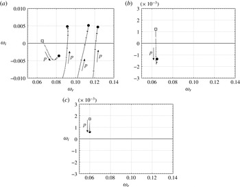
This procedure has been carried out here on the temporal stability spectrum of the BL, and examples for case C01 are reported in figure 13, where three cases are considered: one streamwise section lying in region A, one section in the stable region past region A and one section in region B. In the first case, i.e. figure 13(a), the unstable eigenvalue of the Blasius BL is stabilized by the MVGs, which however destabilize three stable eigenvalues of the Blasius spectrum. As a result, the flow is unstable and three unstable modes can be found. Note that this section is further downstream with respect to that considered in figure 11 and this explains why only three unstable modes are identified instead of four. In the second case, i.e. figure 13(b), it is shown that the unstable mode of the Blasius case is stabilized by the MVGs, and the resulting controlled BL is thus stable. Finally, referring to figure 13(c), in region B the action of the control decreases the growth factor of the unstable mode in the Blasius spectrum, but damping is not sufficient to stabilize it so that the controlled BL is still unstable. The trajectory reported in figure 13(c) highlights that the unstable mode which is identified in region B of the controlled BL is related to the unstable mode of the Blasius BL, and one can be obtained from the other by a continuous deformation of the base flow, as previously pointed out. For this reason we can state that stability region B is the deformation of the instability region of the Blasius BL due to the action of the control, while region A is a new instability region with respect to the Blasius case. This region A is the result of the sudden geometric perturbation of the base flow caused by the MVGs.
Trajectories of selected eigenvalues in the temporal stability spectrum (
 ${\it\alpha}=0.17$
) of the flow obtained by combining linearly the Blasius and the C01 velocity fields through the parameter
 $p$
:
 $p=0$
(filled square, light grey) is the Blasius velocity field and
 $p=1$
(filled circle, dark grey) is the C01 case, the grey graduation being proportional to
 $p$
. (a) Unstable region A (at
 $Re_{x}=1.35\times 10^{5}$
), (b) stable region (at
 $Re_{x}=2.00\times 10^{5}$
), and (c) unstable region B (at
 $Re_{x}=4.70\times 10^{5}$
).

4.3.2. Comparison between stability curves: experiments and DNS
In this section we compare the stability curves obtained in the previous section on the basis of DNS with the available experimental data on the evolution of TS waves in the controlled flow. In the experiments low-amplitude TS waves are excited upstream of the MVGs, at a normalized frequency approximately equal to
 $F=140$
in C01 and
 $F=175$
in C09. The forced amplitude was adjusted to
 $A_{\mathit{TS}}=1.14$
and
 $A_{\mathit{TS}}=1.61$
as a percentage of
 $U_{\infty }$
on branch II for the uncontrolled (Blasius) case and was kept the same for the corresponding controlled cases C01 and C09, respectively. These values of the amplitudes are low enough to expect a good agreement between the TS wave behaviour and what can be estimated by assuming a linearized wave dynamics as done for deriving the stability curves. Thus stability curves are representative of the experimental case provided that the streamwise variations of the base flow are weak enough to justify the local stability analysis, and this might not be fully satisfied in the near-wake past the MVGs. However, as discussed in § 4.1, the region of reversed flow is confined very close to the MVGs, at a distance which is less than
 $h$
, and local stability analysis is started from
 ${\it\chi}\simeq 5$
for both the C01 and C09 cases (corresponding approximately to
 $12h$
for C01 and
 $14h$
for C09). Even though the base flow in the first downstream sections undergoes a relatively rapid variation it is slowed down in the final part of region A, which is the streamwise region of interest for the present analysis where one aim is to identify the streamwise section where the flow becomes convectively stable. The two frequencies excited in the experiments are reported with a horizontal dash-dotted line together with the stability curves in figure 10. This figure indicates that in C01 the excited frequency does not cross the instability region B. Thus, on the basis of the stability curve it is expected that the generated TS wave undergoes an amplification just after the MVGs in region A and, approximately beyond
 $Re_{x}\simeq 1.65\times 10^{5}$
, the TS wave is attenuated as it travels downstream.
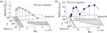
This expected behaviour agrees fairly well with the experimental observations, which are shown in terms of an integrated TS wave amplitude
 $A_{\mathit{TS}}^{yz}$
in figure 14(a) together with the computed stability curves. The amplitude
 $A_{\mathit{TS}}^{yz}$
is evaluated as the integral of the experimental local TS amplitude
 $A_{\mathit{TS}}(x,y,z)$
in the wall-normal direction from the wall up to a fixed distance from the wall
 ${\it\eta}^{\ast }$
and over one period
 ${\it\Lambda}$
in the spanwise direction according to
 $$\begin{eqnarray}A_{\mathit{TS}}^{yz}(x)=\int _{-1/2}^{1/2}\int _{0}^{{\it\eta}^{\ast }}\frac{A_{\mathit{TS}}(x,y,z)}{U_{\infty }}\,\text{d}{\it\eta}\,\text{d}{\it\zeta},\end{eqnarray}$$
where
 ${\it\eta}^{\ast }$
is equal to 9 as for
 $A_{\mathit{ST}}^{\mathit{int}}$
in (4.1). In figure 14 the TS amplitude values are normalized with its most upstream value,
 $A_{\mathit{TS,0}}$
, so that the ratio
 $A_{\mathit{TS}}/A_{\mathit{TS,0}}$
is unity for the first point from the left in the figure. The spatial resolution in the streamwise direction of the experiments does not allow a precise identification of the position where region A finishes, but from the curve reported in figure 14(a) it is plausible that this position is located slightly downstream with respect to the theoretical predictions.
Stability diagrams for cases C01 (a) and C09 (b) in the
 $F$
–
 $\mathit{Re}_{x}$
plane. Grey regions are unstable and white are stable. Symbols correspond to experimental results by Shahinfar et al. (Reference Shahinfar, Fransson, Sattarzadeh and Talamelli2013).

In case C09 the combination of forcing frequency and the streaky base flow also gives rise to an instability region B, as shown in figure 10(b). Thus, it is expected to observe an initial amplification, followed by a subsequent decay after region A. A second amplification is expected when entering instability region B and a final decay on exiting region B. This behaviour is in agreement with experimental observations for case C09, and the experimentally measured amplitude of the TS waves is reported together with the stability curves in figure 14(b). This figure shows that the theoretical stability curve provides an explanation for the experimental behaviour of TS waves. From a quantitative viewpoint, it is difficult to accurately identify the boundaries of the stability regions A and B from the experiments due to the low resolution in the streamwise direction. Nevertheless, discrepancies with DNS are larger for C09 than for C01, and from the analysis of figure 14(b) it is possible to evince that the experimental regions A and B are shifted downstream in the streamwise direction with respect to the theoretical predictions. This behaviour, which is observed in both the C01 and C09 cases, can be explained by the fact that the amplitude of the experimental streaks is always larger than that of the simulated ones. In turn, this may lead to a more extended region A and to a region B which is translated towards higher values of
 $\mathit{Re}_{x}$
, when compared to the theoretical predictions in figure 10. Indeed, as already discussed in the comparison between cases C01 and C09, the base flow modulation by the MVGs is destabilizing for region A and stabilizing for region B.
4.4. Modal analysis of the streamwise evolution of TS waves
As a further assessment of the results obtained by the stability analysis and of their representativeness for the flow past the MVGs, we here compare the eigenmodes from the stability analysis with the available experimental TS wave amplitude in terms of streamwise velocity. As discussed in Piot et al. (Reference Piot, Casalis and Rist2008), this comparison is difficult and questionable in region A which is located just past the MVGs, because in that region many modes are excited by the MVGs and the experimental amplitude is the result of an overlapping of the contributions coming from several modes, including stable ones. In a similar case in Piot et al. (Reference Piot, Casalis and Rist2008) a least-squares approach is employed to approximate the available DNS data with the stability modes in the near-wake of a roughness element, including unstable and stable modes chosen heuristically. In fact, a precise criterion for the selection of stable modes to include in that procedure does not exist, although the success of the procedure depends on the inclusion of representative stable modes.
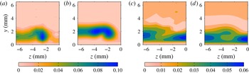
Comparison between experimental TS wave amplitudes of the streamwise velocity component and the norm of the streamwise velocity of the unstable mode of region B: (a,b) correspond to C01 at
 $\mathit{Re}_{x}=1.702\times 10^{5}$
and (c,d) to C09 at
 $\mathit{Re}_{x}=1.88\times 10^{5}$
. (a,c) Experimental, (b,d) stability analysis.

The situation is different further downstream. For case C09, experimental TS waves enter the unstable region B, where only one mode is amplified. For this reason, just after region B it is expected that the contribution to the experimental amplitude comes entirely from the unstable mode identified in region B. This is confirmed in figure 15(c,d), where the unstable mode of region B is followed in the streamwise direction up to
 $\mathit{Re}_{x}=1.88\times 10^{5}$
and the norm of its streamwise velocity component is plotted and compared with the available experimental amplitudes (case C09). We consider only the streamwise velocity component because it is the only one available from the experiments. The eigenmode amplitude is scaled so as to compare quantitatively with the experimental map. The comparison of the eigenmode against the experiments is fairly good, the shape of the mode being very similar to the experimental amplitudes, and discrepancies are mainly in the disturbance field distant from the wall. This difference can have several causes. Apart from the many possible and uncontrollable sources of errors both in the experiments and in the simulations already mentioned in § 4.2, the position of the wall is not identified accurately in the experiments, due to the technical problems in measuring velocities very close to the plate wall; thus experimental flow fields reported in figure 15(c,d) can be slightly shifted with respect to their real position. Moreover, even a very small pressure gradient in the experiments can have a slight effect on the thickness of the BL at the large distance from the leading edge considered, due to the fact that it has acted over a long distance. Concerning possible leading-edge effects giving rise to some degree of mismatch in direct comparisons with theoretical predictions, which can be compensated by the introduction of a virtual origin for the experimental BL, it has been verified that they are minimal for the cases considered and cannot explain the discrepancies at issue here. Nevertheless, despite the observed discrepancy, figure 15(c,d) confirms that the identified eigenmode is representative for the experimental flow dynamics when the flow is excited by a controlled and small-amplitude TS wave, and this further validates the results of the stability analysis.
Concerning case C01, the excited TS waves do not cross region B. Nevertheless, it is expected that, although in region A several modes are excited at the same time, at a sufficient distance downstream of the MVGs, well downstream of region A, the experimental root-mean-square (r.m.s.) distribution of the streamwise velocity is dominated by the contribution of the least-damped eigenmode in space. As a confirmation, the norm of the streamwise velocity of this mode, properly scaled in amplitude, is reported and compared to the experimental r.m.s.-distribution at
 $\mathit{Re}_{x}=1.702\times 10^{5}$
in figure 15(a,b). As for C09, also in this case the eigenmode compares satisfactorily with the experimental r.m.s.-distribution. The agreement is not as good as for the C09 case because in C09 the waves cross region B, which is a selective amplifier for the identified eigenmode. Conversely, in C01 the mode is not amplified after region A, and it is expected to emerge only because the other excited modes decay more rapidly. Like C09, in C01 differences are also mainly in the region distant from the wall, and the discussion above for C09 also applies to C01.
5. Conclusions
This paper is dedicated to simulating and to investigating the stability properties of flat-plate BLs, in which MVGs are installed in a spanwise array at a prescribed distance from the plate leading edge. The objective of the MVGs is to generate steady and stable velocity modulations that stabilize TS waves and reduce their growth rate in comparison with the uncontrolled case, i.e. a Blasius BL. It is shown here that linear stability analysis is able to explain the particular behaviour of TS waves observed in the experiments for two configurations of interest identified in previous investigations. In particular, a first region of instability is identified in the controlled case which starts just after the MVGs and where more unstable modes are found, which are excited by the geometric discontinuity associated with the MVGs. This region has no counterpart in the Blasius BL, and in the cases considered the region ends at a given distance from the MVGs. The streamwise extent of the unstable region increases with the streak amplitude. After this instability region, the flow becomes convectively stable, and this happens at a distance from the leading edge at which the Blasius BL would be unstable. Further downstream, the velocity modulation generated by the MVGs weakens and hence also the stabilizing effect. This may cause the flow instability to appear in a way which is shown to be closely related and very similar to the onset of instability in a Blasius BL. The theoretical predictions of the stability analysis, summarized in a stability curve for each flow configuration considered, are based on the simulated flow fields.
Simulations are validated against experiments. The experimental behaviour of small-amplitude TS waves is in agreement with the theoretical predictions found by stability analysis. As a further confirmation, it is shown that the TS wave amplitude of the experimental flow fields, in which controlled TS waves are artificially excited, agree reasonably well with the shape of the identified unstable or least-damped stable modes when considered sufficiently far downstream from the MVGs.
To the authors’ knowledge, this paper provides for the first time the stability curves for the BL controlled by MVGs, which has been shown in previous experimental works to be a promising method to delay transition in BLs. The fact that the behaviour of TS waves is related here to the results of a local stability analysis and to the behaviour of identified unstable modes, which is the core of the present paper, is important knowledge which can drive future design of new BL modulators improving the performances of MVGs. Finally, besides the physical and fundamental interest of the results presented, a secondary goal of this paper is to validate the methodology based on a bi-global stability analysis, which is not original (see e.g. Piot et al. Reference Piot, Casalis and Rist2008), for cases in which passive BL control is carried out by MVGs. In the present version, where DNS is needed, the methodology adopted here can save a significant amount of experimental work in the characterization of the behaviour of small-amplitude TS waves travelling in the controlled flow. However, if DNS is replaced by a three-dimensional BL solver which could take into account the available experimental results, the methodology presented could lead to very fast and cheap prediction of the stability properties of controlled configurations, saving computational and experimental time. This is one of the objectives of future developments of the present research activity, which could allow a feasible optimization of the MVG configuration to be carried out, taking into account several free parameters.
Acknowledgements
The authors wish to acknowledge PRACE for awarding access to resource Fermi based in Italy at Cineca. J.H.M.F. acknowledges the European Research Council for their financial support of the AFRODITE project through a Starting Independent Researcher Grant. S.C. acknowledges travelling support by the C. M. Lerici Foundation.