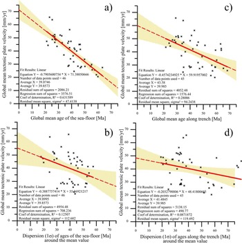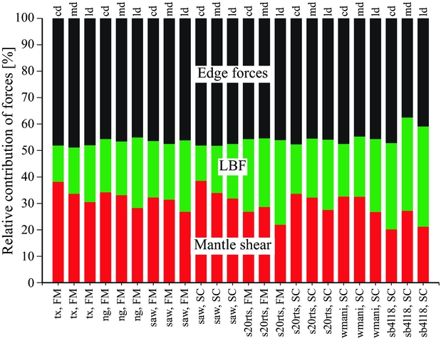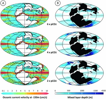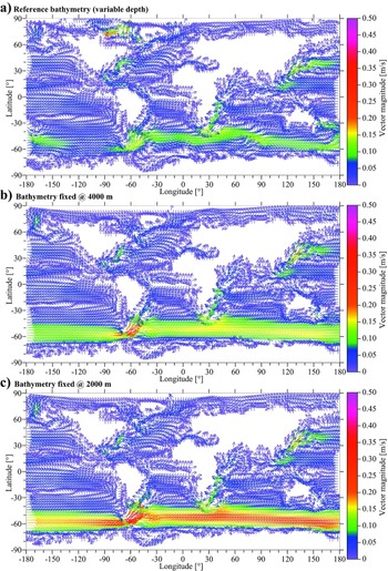


1. Introduction
Plate tectonic models are tools that permit, on the one hand, the returning of data to their past plate tectonic configuration, and on the other hand, the provision of a global view to better understand the evolution of the Earth throughout geological time. Such a tool is complex to generate since it involves integrating many concepts of different fields of geosciences (palaeontology, sedimentology, geophysics (seismic tomography, gravimetry, palaeomagnetism . . .), rheology, geochemistry (dating, source rocks . . .), etc), and being consistent with the data that these disciplines provide. In addition, such work must be conducted on a global scale, over the longest possible geological time periods, in order to integrate aspects that correspond to tectonic heritage. Finally, one must not lose sight that plate tectonic models are an interpretation made by some at a global scale from regional interpretations sometimes made by others, which are themselves inferred from local data acquired over the years by the scientific community.
The present paper aims to (1) thank the scientists who have embarked on this ambitious challenge through a review of existing models, (2) compare the methods used to create these models, and (3) suggest ways these reconstructions can be used in the future to go further in order to better understand the evolution of the planet.
2. Historical background
Plate tectonics is the surface expression of the planet of mechanisms related to the cooling of the Earth. The theory is relatively recent, because the wealth of plate tectonics goes far beyond that of a simple kinematic theory.
Indeed, there is still a lot of confusion – even in the mind of some specialists – between the continental drift theory as presented by Alfred Wegener (Reference Wegener1912) and the plate tectonics theory as propounded in pioneering papers (Wilson, Reference Wilson1965; McKenzie & Parker, Reference McKenzie and Parker1967; Morgan, Reference Morgan1968; Le Pichon, Reference Le Pichon1968; Isacks, Oliver & Sykes, Reference Isacks, Oliver and Sykes1968; Vine & Hess, Reference Vine and Hess1968).
The fact that the landmasses had been moving on the surface of the globe is an ancient concept. In the sixteenth century, Abraham Ortelius (a Dutch cartographer) and Sir Francis Bacon (an English scientist and philosopher) noted the similarity of the American and African coasts, and hypothesized that these continents were once together (Ortelius, Reference Ortelius1570; Bacon, Reference Bacon1620). Although Wegener (Reference Wegener1912, Reference Wegener1915) had been able to gather a number of arguments to support his theory of continental drift, it was at first widely contested – quite rightly – in regards to the mechanisms involved in the movement. The model of mantle convection shown by Hess (Reference Hess, Engel, James and Leonard1962), which showed great similarities with assumptions made by Holmes (Reference Holmes1913, Reference Holmes1944), includes the fundamental basics that surface kinematics are linked to deep movements. When Dietz (Reference Dietz1961) introduced the term ‘sea-floor spreading’ and Oliver & Isacks (Reference Oliver and Isacks1967) interpreted the Wadati-Benioff planes (Wadati, Reference Wadati1928, Reference Wadati1929, Reference Wadati1931; see also Frohlich, Reference Frohlich1987; Benioff, Reference Benioff1955) as the traces of oceanic lithosphere returning back into the mantle (which is now called a ‘subduction zone’), they defined the critical limits of what McKenzie & Parker (Reference McKenzie and Parker1967) called ‘plates’.
In the case of continental drift, the authors have focused on the kinematics of the continents (disregarding sea-floor and unrelated to the mantle), while in the case of plate tectonics, the important thing is not so much the continents but the plates and in particular the plate boundaries. These are seismically active and are namely the rift axes, the oceanic ridges, the transform faults, the subduction zones and obduction zones (potentially adduction zones, see Shemenda, Reference Shemenda1985, Reference Shemenda1993), and the collision zones. All other geological boundaries are intraplate features and passive from a geodynamical point-of-view. Of course, some boundaries are relatively diffuse in space and time. In time: Will such-and-such rift zone become abandoned or not? Is such a collision zone still active or has the ‘slab’ detached so that the boundary has become an intraplate suture? In space: The definition of plate boundaries is very much a matter of scale, but also depends upon which data (seismic, GPS, etc.) plates are delimited. For example, the NUVEL-1 model defined 12 large plates (e.g. DeMets et al. Reference DeMets, Gordon, Argus and Stein1994) while Bird (Reference Bird2003) proposed an Earth with 52 plates.
2.a. Tectonics, kinematics, geodynamics: definition
The three terms – tectonics, kinematics and geodynamics – are widely used in geosciences, but not always with the same meaning. It is therefore necessary to clarify the meaning given here.
Tectonics – from the Greek τἔκτων [tektōn] meaning ‘builder, carpenter’ – examines the structures, the geological architectures. It therefore describes states, at given times, and the causes that produced them. Kinematics – from the Greek κινημα [kinema] meaning ‘movement’ – is interested in movements, regardless of the reasons. So it describes as much the ‘continental drift’ that is the movement of tectonic plates, defining paths (and verifying that the geometries of the plates, for example, are consistent with the proposed movements), Euler poles and velocities. Lastly, geodynamics – from the Greek δὔναμις [dunamis] meaning ‘power’ – is interested in the dynamics of the various parts that envelope the globe (i.e. lithosphere and asthenosphere: internal geodynamics; and hydrosphere and atmosphere: external geodynamics). It therefore considers objects that change over time (i.e. as opposed to static), and considers not only the movements but also their changes, especially the forces (in particular forces acting at plate boundaries) that allow both movements and changes.
To these words, the concept of ‘geodynamic environments’ should be added (see in particular C. Hochard, unpub. Ph.D. thesis, Univ. Lausanne, 2008), which refers to geological units subject to the same regional stress field related to the movement of the plates to which they belong (see below).
2.b. The engine of plate tectonics
The continental drift theory was abandoned in particular because it represented the continents floating on the surface of the mantle (what some people – especially in the media – still readily see nowadays as a magma ocean) and it did not propose a mechanism for the observed drift.
However, it must be acknowledged that the ‘engine of plate tectonics’ remains a matter of debate, and an active field of research (see Section 5). Of course, as stated by Turcotte & Schubert (Reference Turcotte and Schubert2002, p. 54) for instance, ‘the only source of energy of sufficient magnitude is heat from the interior of the Earth’. In addition, these authors recalled that a very little part of this energy is converted into the motion of tectonic plates since ‘the energy associated with seismicity, volcanism and mountain building is about 1% of the heat flow to the surface’.
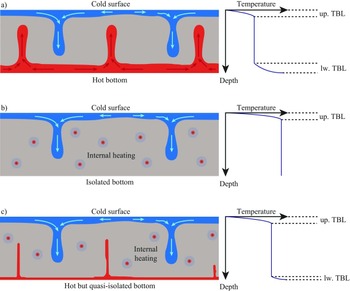
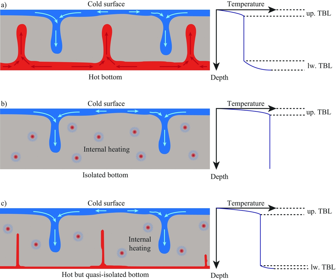
Indeed, it is now accepted that the mantle is solid and affected by the movement of convection (e.g. Hess, Reference Hess, Engel, James and Leonard1962; Rayleigh Number >> 103, and see numerical simulations by Schmalzl, Houseman & Hansen, Reference Schmalzl, Houseman and Hansen1996 or Bunge, Richards & Baumgardner, Reference Bunge, Richards and Baumgardner1997 and later works such as Breuer et al. Reference Breuer, Wessling, Schmalzl and Hansen2004 or Davies et al. Reference Davies, Davies, Bollada, Hassan, Morgan and Nithiarasu2013, for instance). However, the analogy – often made for outreach or education purposes (see Section 2.c) – with boiling water in a pan is wrong because it merely implies the presence of a lower thermal boundary layer due to heating the bottom (in contact with the stovetop) and a thermal boundary layer because of the rapid cooling due to contact with the air (Fig. 1a). For the Earth, the heat source, radioactivity, is essentially internal to the mantle. Therefore, if the descent of material, that which is colder, is active, the rise of hot material is not (Fig. 1c), except in association with hotspots. This phenomenon is observed by seismic tomography where the ‘cold zones’ (i.e. seismically slower) are visible below subduction zones, whereas no warm rise is observed at the mantle scale below oceanic ridges, except in association with hotspots (e.g. Grand, van der Hilst & Widiyantoro, Reference Grand, van der Hilst and Widiyantoro1997). These phenomena of active descent and passive rising (excluding hotspots) are also verified by numerical modelling of the mantle (e.g. Davies et al. Reference Davies, Goes, Davies, Schubert, Bunge and Ritsema2012; Crameri et al. Reference Crameri, Tackley, Meilick, Gerya and Kaus2012). It should be noted, however, that, although the amount of cold material descending seems largely superior to the amount of hot material actively rising, the action of the latter is possibly fundamental to plate tectonics (Courtillot et al. Reference Courtillot, Jaupart, Manighetti, Tapponnier and Besse1999; Cande & Stegman, Reference Cande and Stegman2011; Brune, Popov & Sobolev, Reference Brune, Popov and Sobolev2013).
Three types of thermal convection, after Thomas (Reference Thomas2010) but translated in English. (a) In case 1, the medium is heated from below (red plumes) and cooled from above (blue plumes): two thermal boundary layers are generated (up. TBL – upper thermal boundary layer; lw. TBL – lower thermal boundary layer); the matter, in the upper part, which is denser because it is cooler, actively plunges, while the matter, in the lower part, which is less dense because it is hotter, actively rises. In between, the matter moves little and has a quasi-constant temperature. (b) In case 2, heat production is in the body, so there is no matter that is hotter (less dense) than the surrounding; the matter only rises passively to compensate for the active plunging of cold matter. (c) Case 3 is intermediate between case 1 and case 2 with a large amount of active plunging and much less active rising. This case is proposed to correspond to the Earth's system, with the Earth's core releasing little heat, and radioactive elements heating the heart of the mantle.
2.c. Plate tectonics and misleading outreach
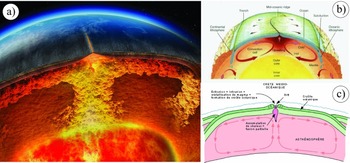
Plate tectonics, its mechanisms and implications are usually and unfortunately not properly broadcast, particularly in the media and to the general public. Nevertheless, it is our responsibility to share our knowledge, and especially not to perpetuate misconceptions. Many images – such as those in Figure 2 – from books (e.g. Hewitt et al. Reference Hewitt, Lyons, Suchocki and Yeh2007, fig. 22.16), television programmes (e.g. BBC documentary film ‘Earth: The Power of the Planet’; http://www.bbc.co.uk/programmes/b008fdjy) or worse, on the internet (clip from National Geographic ‘The Early Earth and Plate Tectonics’; https://www.youtube.com/watch?v=QDqskltCixA), are false or misleading.
Examples of erroneous or misleading representations of plate tectonics on Earth. (a) Picture from BBC documentary film ‘Earth: The Power of the Planet’, equally visible on http://www.youtube.com/watch?v=ryrXAGY1dmE. (b) Illustration by Götz Bokelmann formerly on http://www.dstu.univ-montp2.fr/PERSO/bokelmann/convection.gif and still visible on over a hundred websites worldwide. (c) Illustration by Pierre-André Bourque, visible on http://www2.ggl.ulaval.ca/personnel/bourque/intro.pt/planete_terre.html.

In all these images (Fig. 2), the mantle – shown in red – seems to ‘boil’ and the mid-oceanic ridge is located in the centre of the system as if it plays a central role. The arrows showing the mantle convective motions are large compared to the movement of the tectonic plates. All this suggests a boiling mantle of magma, with active rise of material, causing the separation of the continents.
Such images of the interior of the planet, associated with some palaeogeographic reconstructions (see below) showing continents drifting on the surface of the globe, send the wrong message not only to the media and the general public, but even to our students and the scientific community. They should be banned.
3. Plate tectonic reconstructions
The idea of reconstructing the position of continents at different geological times is relatively old. Although Wegener (Reference Wegener1912, Reference Wegener1915) is considered the father of continental drift and notably introduced the term ‘Pangaea’, Du Toit (Reference Du Toit1937) is the one who presented detailed evidence that the southern continents were once united and then subsequently dispersed. He produced the first plausible maps of Gondwana that strongly resemble the currently accepted views as to its original shape. It should be noted that the term Gondwana should be preferred over Gondwanaland introduced by Suess (Reference Suess1892) – along with the name of the Tethys Sea – as Gondwana means the forest or land [-wâna] of the Gond people [Gond-]. It is therefore redundant to speak of Gondwanaland, which literally means ‘the land of the land of the Gonds’. Meert (Reference Meert2012) positively discussed the problems of spelling and meaning of various terms used for past reconstructions.
Since the advent of plate tectonics, many models have been proposed. The first is probably that of Dewey & Bird (Reference Dewey and Bird1970). Only models that are proposed at the global scale and constructed using spherical geometries (whatever the projection used afterwards for the presented maps) are considered herein, although those are often based on regional models such as, for example, Ziegler (Reference Ziegler1982), Cope, Ingham & Rawson (Reference Cope, Ingham and Rawson1992), Dercourt, Ricou & Vrielynck (Reference Dercourt, Ricou and Vrielynck1993), Dercourt (Reference Dercourt2000), Gaetani, Dercourt & Vrielynck (Reference Gaetani, Dercourt and Vrielynck2003) and Cavazza et al. (Reference Cavazza, Roure, Spakman, Stampfli and Ziegler2004) for Europe, Barker (Reference Barker2001) and Eagles & Jokat (Reference Eagles and Jokat2014) for the Scotia Sea, Pindell & Kennan (Reference Pindell, Kennan, James, Lorente and Pindell2009) for the Caribbean, Gaina et al. (Reference Gaina, Müller, Royer, Stock, Hardebeck and Symonds1998a,b) for the Tasman Sea, Metcalfe (Reference Metcalfe2011) and Hall (Reference Hall2012) for Asia, etc.
3.a. List of global ‘plate tectonic’ models and related plate modelling software
There are models created in academic institutions and others developed within private companies, including oil companies. For the latter, it is extremely difficult to obtain general information about the models, and even more so for technical information. However, existing models are, as far as I know, the following:
(1) The Cambridge Paleomap Systems Ltd: Alan Smith is one of the first global plate modellers (Smith et al. Reference Smith, Briden, Drewry and Hughes1973; see also Smith, Smith & Funnell, Reference Smith, Smith and Funnell1994). His plate tectonic modelling software, ‘Time trekker’, was available commercially for many years. He recently sold the rights to his plate tectonic model and software to FrogTech (http://www.frogtech.com.au; see below).
(2) The PaleoMap Project: Christopher Scotese (http://www.scotese.com and references therein; Fig. 3a) worked on global reconstructions as early as in the 1970s (Scotese & Baker, Reference Scotese and Baker1975; Scotese, Reference Scotese1976). He collaborated with many other researchers and stimulated new axes of research in disciplines as diverse as palaeomagnetism (e.g. Van der Voo, Scotese & Bonhommet, Reference Van der Voo, Scotese and Bonhommet1984), the tectonic fabric of the ocean basins (e.g. Gahagan et al. Reference Gahagan, Scotese, Royer, Sandwell, Winn, Tomlins, Ross, Newman, Müller, Mayes, Lawver and Heubeck1988), lithostratigraphic indicators (e.g. Parrish, Ziegler & Scotese, Reference Parrish, Ziegler and Scotese1982; Boucot, Reference Boucot1999; Boucot et al. Reference Boucot, Xu, Scotese and Morley2013), biogeography (Rowley et al. Reference Rowley, Raymond, Totman Parrish, Lottes, Scotese and Ziegler1985; McKerrow & Scotese, Reference McKerrow and Scotese1990) and in particular palaeogeographic modelling (Golonka, Ross & Scotese, Reference Golonka, Ross, Scotese, Embry, Beauchamp and Glass1994), and even palaeoclimate modelling (Ross, Scotese & Otto-Bliesner, Reference Ross, Scotese and Otto-Bliesner1992; see also Klein, Reference Klein1994 and references therein).
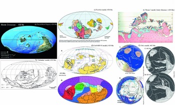
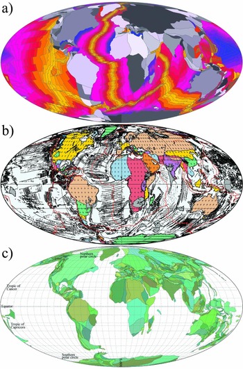
Examples of reconstructions according to different models. (a) 458 Ma reconstruction after the PaleoMap project (http://www.scotese.com/newpage1.htm); (b) 450 Ma reconstruction after the ‘Golonka’ model (Golonka, Reference Golonka2007a, fig. 26); (c) 450 Ma reconstruction after the PLATES project (http://www-udc.ig.utexas.edu/external/plates/450.htm); (d) 410 Ma reconstruction after the EarthByte project (Domeier & Torsvik, Reference Domeier and Torsvik2014, fig. 5), with (A) the plate tectonic reconstruction, and (B) the associated plate velocity field; (e) Early Silurian (~ 438 Ma) reconstruction after the ‘Ronov’ model (Ronov, Khain & Seslavinsky, Reference Ronov, Khain and Seslavinsky1984, map p. 57); (f) 442 Ma reconstruction after the UNIL model, with several views since mollweide projections are not available anymore: (A) the reconstruction as done before 2004 (Stampfli et al. Reference Stampfli, Borel, Marchant, Mosar, Rosenbaum and Lister2002; Stampfli & Borel, Reference Stampfli, Borel, Cavazza, Roure, Sparkman, Stampfli and Ziegler2004); (B) as done after 2004 in south pole view (Stampfli et al. Reference Stampfli, Hochard, Vérard, Wilhem and von Raumer2013, fig. 5; © Neftex, v.2010); and (C) equatorial view (C. Wilhem, unpub. Ph.D. thesis, Univ. Lausanne, 2010, fig. 5.18); in (D) reconstruction at 420 Ma as part of the same figure (C. Wilhem, unpub. Ph.D. thesis, Univ. Lausanne, 2010, fig. 5.18), and it also better compares with the EarthByte project (d).
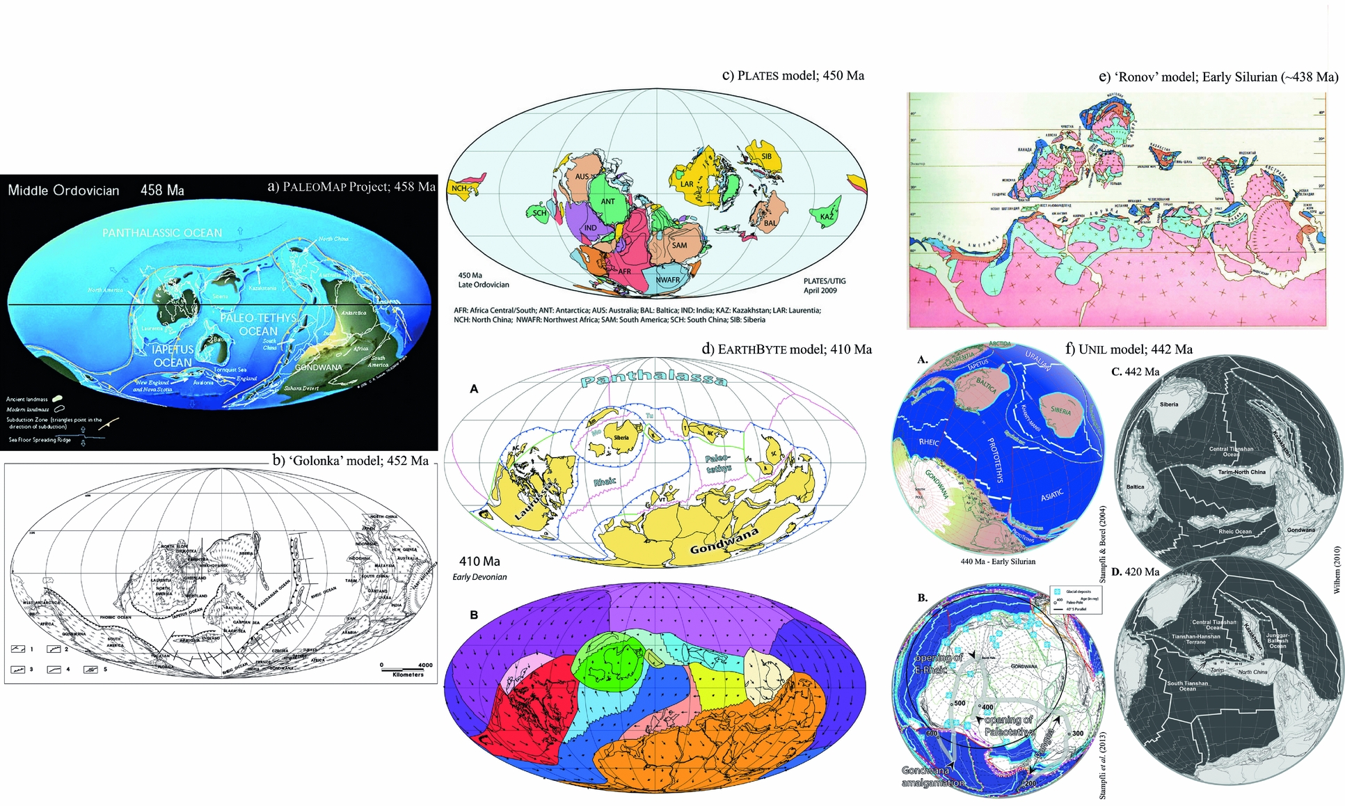
The website (http://www.scotese.com) offers 17 global maps from 650 Ma to the present day and even three maps for the potential evolution of the Earth in the future at +50 Ma, +100 Ma and +250 Ma. Google Earth® versions can additionally be downloaded on http://globalgeology.com and animations can be viewed from other websites, in particular on YouTube® (https://youtube.com/user/cscotese).
It is also worth noting that the plate tectonic reconstructions in the models mentioned below in (3), (5), (6), (8), (14a) and (14b) are based on Scotese global plate tectonic models. The original Scotese modelling software (Scotese, Reference Scotese1976) was the basis of other modelling software programs, including Terra Mobilis (1985) for Macintosh, Plate Trekker (1994) for Windows, PaleoGIS (2000) for ArcGIS and PointTracker (2001–2010) for iMac, and was the design inspiration for software developed by the PLATES and GPlates projects (C. Scotese, pers. com. 2017).
(3) The ‘Ronov’ models (Ronov, Khain & Seslavinsky, Reference Ronov, Khain and Seslavinsky1984; Ronov, Khain & Balukhovsky, Reference Ronov, Khain and Balukhovsky1989; Fig. 3e) are poorly known because they are difficult to access and in Russian. The atlases are, however, interesting because they are proposed in two parts: one part where the maps define lithofacies on the current configuration of the Earth for the chosen ages; and a second part where the lithofacies maps are returned to their original configurations in the past. Global reconstructions themselves include 19 maps, 7 for the Vendian–Palaeozoic and 12 for the Mesozoic–Cenozoic periods.
(4) A number of global reconstructions at least from Permian to Cretaceous times have also been proposed mainly by Nikolai Chumakov and Mikhail Zharkov (Zharkov, Murdmaa & Filatova, Reference Zharkov, Murdmaa and Filatova1995, Reference Zharkov, Murdmaa and Filatova1998a,Reference Zharkov, Murdmaa and Filatovab; Zharkov & Chumakov, Reference Zharkov and Chumakov2001; Chumakov & Zharkov, Reference Chumakov and Zharkov2002, Reference Chumakov and Zharkov2003; Chumakov, Reference Chumakov2004). However, it is unclear how many maps were actually created because those lithofacies maps – compiling reconstructions by Ziegler, Scotese, Golonka, Dercourt, etc. and atlases from the Soviet Union – were published piecemeal predominantly in numerous papers of a journal named ‘Stratigraphy and Geological Correlation’, which is a translation of the Russian journal ‘Stratigrafiya, Geologicheskaya Korrelyatsiya’. No website, in particular, gathers those reconstructions.
(5) Palaeogeographic maps of the Colorado Plateau Geosystems, Inc.™ (hereafter named CPGeosystems maps), which are based on the Scotese plate tectonic reconstructions, were probably, with those of the PaleoMap Project, the most widely used maps in the academic world, but also by the media and the general public. Indeed, these maps created by Ronald Blakey (e.g. Blakey, Reference Blakey, Fielding, Frank and Isbell2008) are particularly attractive because palaeogeographies are portrayed with Adobe® Photoshop® by taking the textures of the present-day topography. The rendering is beautiful.
However, the CPGeosystems model, which was until recently available on their website as 27 global maps from 600 Ma to the present day, is not available anymore, and has been superseded by copyrighted “Deep Time Maps” (http://deeptimemaps.com/).
(6) The ‘Golonka’ model (in particular Golonka et al. Reference Golonka, Ross, Scotese, Embry, Beauchamp and Glass1994; Golonka, Reference Golonka2000, Reference Golonka2007a,Reference Golonkab,Reference Golonkac, Reference Golonka2009) and ‘Vrielynck’ model (Vrielynck & Bouysse, Reference Vrielynck and Bouysse2003) are palaeogeographic reconstructions and lithofacies maps whose ‘tectonic background’ is largely based on the PLATES Project and PaleoMap Project.
The ‘Golonka’ model (as visible in Golonka, Reference Golonka2007a,Reference Golonkab,Reference Golonkac and Reference Golonka2009; Fig. 3b) includes 32 global maps from 544 Ma to the present day. The ‘Vrielynck’ model is restricted to 11 global maps from 250 Ma to the present day.
(7) The PLATES project (http://ig.utexas.edu/marine-and-tectonics/plates-project/; Fig. 3c), started at the Institute for Geophysics of the University of Texas at Austin (UTIG) by J. G. Sclater, C. R. Scotese and L. A. Lawver in 1984, assembled the first global database of magnetic picks and isochrons (Scotese et al. Reference Scotese, Gahagan, Larson, Scotese and Sager1988). This database of marine magnetic data was used to produce global plate tectonic reconstructions and was the basis of the Global Isochron Chart (Royer et al. Reference Royer, Müller, Gahagan, Lawver, Mayes, Nürnberg and Sclater1992). Dietmar Müller, who later started the EarthByte Project (below), was an early member of the PLATES project.
The project, published by Dalziel (Reference Dalziel1997), continues to develop under the direction of, in particular, Lawrence Lawver, Ian Dalziel, Ian Norton and Lisa Gahagan. A PowerPoint® animation (http://www-udc.ig.utexas.edu/external/plates/recons.htm) shows global maps every 10 million years from 750 Ma to the present day, and even a reconstruction at +100 Ma in the future.
(8) The Paleo-Continental Map Editor (http://www.serg.unicam.it/Intro-Reconstr.html) is actually software developed to produce reconstructions at any age between 200 Ma and the present (note that the website offers an online tool). The software uses the reconstruction techniques of the PaleoMap Project and is based on the rotation poles of Schettino & Scotese (Reference Schettino and Scotese2005). However, on this basis, Schettino & Turco (Reference Schettino and Turco2011) have produced remarkable and refined high-resolution reconstructions in time (every million years) concerning the opening the Atlantic and Alpine Tethys region.
(9) Another online tool for generating reconstructions from 150 Ma to the present is available from the Ocean Drilling Stratigraphic Network (ODSN website: http://www.odsn.de/odsn/services/paleomap/paleomap.html). The website describes well the methods and datasets used to allow the generation of those maps (see http://www.odsn.de/odsn/services/paleomap/about_map.html). However, I am personally aware of only one publication that used this tool: Hay et al. (Reference Hay, DeConto, Wold, Wilson, Voigt, Schulz, Rossby-Wold, Dullo, Ronov, Balukhovsky, Söding, Barrera and Johnson1999), which also details well the techniques employed for proposing both the plate tectonic maps and palaeogeographic maps for the Cretaceous period. It is noteworthy that this paper probably refers to the first model to generate a global synthetic topography with an associated digital elevation model.
(10) Torsvik & Smethrust (Reference Torsvik and Smethrust1999) developed the GMAP software, designed to process palaeomagnetic data and to reposition continents accordingly. Although GMAP has been improved (see the GMAP2015 version: http://www.earthdynamics.org/resources.html) and although the software is still widely used by the scientific community – in particular by palaeomagneticians – to propose many reconstructions of the Earth in the past, the ‘routines are currently being ported to GPlates (see below)’ according to Trond Torsvik, and GPlates is likely to supersede GMAP in the future.
(11) The EarthByte Project (http://www.earthbyte.org), led by Dietmar Müller, is linked to lines of research in many disciplines (mantle convection, continental deformation, palaeoclimate modelling, etc.), and generated a truly impressive number of scientific publications. The EarthByte Plate Tectonic Model (http://www.earthbyte.org/Resources/global_plate_model_ESR12.html) is created using the GPlates software (http://www.gplates.org/) developed under the leadership of Dietmar Müller, Mike Gurnis and Trond Torsvik (see also Williams et al. Reference Williams, Müller, Landgrebe and Whittaker2012). The EarthByte Model is created in particular on the basis of the age grid model of Royer et al. (Reference Royer, Müller, Gahagan, Lawver, Mayes, Nürnberg and Sclater1992) updated by Müller et al. (Reference Müller, Roest, Royer, Gahagan and Sclater1997, Reference Müller, Sdrolias, Gaina and Roest2008) and Seton et al. (Reference Seton, Müller, Zahirovic, Gaina, Torsvik, Shephard, Talsma, Gurnis, Turner, Maus and Chandler2012), and the polar wander paths of Torsvik et al. (Reference Torsvik, Müller, Van der Voo, Steinberger and Gaina2008, Reference Torsvik, Van der Voo, Preeden, Mac Niocaill, Steinberger, Doubrovine, van Hinsbergen, Domeier, Gaina, Tohver, Meert, McCausland and Cocks2012).
The EarthByte Model (http://www.earthbyte.org/Resources/global_plate_model_ESR12.html) was presented by Seton et al. (Reference Seton, Müller, Zahirovic, Gaina, Torsvik, Shephard, Talsma, Gurnis, Turner, Maus and Chandler2012) in the form of 11 maps of plate tectonic reconstructions from 200 Ma to the present day every 20 Ma.
However, Domeier & Torsvik (Reference Domeier and Torsvik2014) showed nine additional maps from 410 Ma to 250 Ma (Fig. 3d), and Cocks & Torsvik (Reference Cocks and Torsvik2011, Reference Cocks and Torsvik2013) presented palaeogeographic maps from 510 Ma to 250 Ma for Laurentia and eastern Asia, and Torsvik & Cocks (Reference Torsvik, Cocks, Hinsbergen, Buiter, Torsvik, Gaina and Webb2011, Reference Cocks and Torsvik2013) for Gondwana. These maps have just been compiled and reworked in Torsvik & Cocks (Reference Torsvik and Cocks2017).
(12) The UNIL model (https://www.unil.ch/iste/en/home/menuinst/recherche/geology-and-geodynamics-of-mountain-belts/gerard-stampfli.html) is a model of plate tectonics created under the leadership of Gérard Stampfli (e.g. Stampfli & Borel, Reference Stampfli and Borel2002, Reference Stampfli, Borel, Cavazza, Roure, Sparkman, Stampfli and Ziegler2004). The model very much evolved between 2004 and 2010 with the creation of many tools under ArcGIS® (C. Hochard, unpub. Ph.D. thesis, Univ. Lausanne, 2008), and by including the reconstructions of the Pacific and Caribbean (K. Flores-Reyes, unpub. Ph.D. thesis, Univ. Lausanne, 2009), Siberia and eastern Asia throughout Palaeozoic time (Ferrari, Hochard & Stampfli, Reference Ferrari, Hochard and Stampfli2008; and C. Wilhem, unpub. Ph.D. thesis, Univ. Lausanne, 2010; Wilhem, Windley & Stampfli, Reference Wilhem, Windley and Stampfli2012), southern Gondwana (Vérard & Stampfli, Reference Vérard and Stampfli2013a,b) and northern Gondwana (Stampfli et al. Reference Stampfli, Hochard, Vérard, Wilhem and von Raumer2013; Fig. 3f).
In 2010–2011, the model had 46 plate tectonic maps from 600 Ma to the present day covering 100% of the Earth's surface, i.e. including the palaeo-Pacific and Panthalassic realms. However, the UNIL model was sold to the company Neftex Petroleum Consultants Ltd. (now Halliburton: http://www.halliburton.com) to be included in their Earth Model package (see below), and the UNIL model is thus no longer available to academics.
Nevertheless, rather old (c. 2007–2008 version) maps are available at https://www.unil.ch/iste/en/home/menuinst/recherche/geology-and-geodynamics-of-mountain-belts/gerard-stampfli.html and more recent maps are shown in numerous papers and appendices of Ph.D. theses (e.g. K. Flores-Reyes, unpub. Ph.D. thesis, Univ. Lausanne, 2009; C. Wilhem, unpub. Ph.D. thesis, Univ. Lausanne, 2010; P. Webb, unpub. Ph.D. thesis, Univ. Cardiff, 2012).
(13) There are other global models, usually entirely based on palaeomagnetic data and mostly created using GMAP, including the reconstructions of Li et al. (Reference Li, Bogdanova, Collins, Davidson, De Waele, Ernst, Fitzsimons, Fuck, Gladkochub, Jacobs, Karlstrom, Lu, Natapov, Pease, Pisarevsky, Thrane and Vernikovsky2008) for the Neoproterozoic (12 global maps from 1100 Ma to 530 Ma), McElhinny, Powell & Pisarevsky (Reference McElhinny, Powell and Pisarevsky2003) for the Palaeozoic (10 global maps from 530 Ma to 320 Ma) and Fluteau (Reference Fluteau, Duplessy and Ramstein2013) who used the aforementioned reconstructions and extended them to the present (16 global maps from 1000 Ma to 0 Ma). It is worth pointing out, however, that though Fluteau (Reference Fluteau2001, Reference Fluteau, Duplessy and Ramstein2013), for example, produced global reconstructions, his work is largely focused on other issues, including climate modelling in the past and implications of tectonic–climate relationships (the same is true for others; reconstructions exist from Hallam, Reference Hallam1985 to Hay & Flögel, Reference Hay and Flögel2012 for instance).
(14) The list of commercial models is much less clear. There are probably a number of proprietary models, particularly in the major oil companies, but for which no information is disclosed. Among the models related to the consulting business, the following can be quoted:
(a) PaleoGIS™, owned by the Rothwell Group (http://www.paleogis.com); although the model has largely evolved, it is historically derived from the UTIG model and the PaleoMap Project. In fact, strictly speaking, the name PaleoGIS™ corresponds to the software while the model is called PaleoGlobe. Additional products are used to create animations (PaleoRun) or to work via the web (PaleoWeb), and even to define palaeoclimate maps (PaleoClimate) on the basis of the work of Malcolm Ross in particular (e.g. Ross, Scotese & Otto-Bliesner, Reference Ross, Scotese and Otto-Bliesner1992; Ross & Scotese, Reference Ross and Scotese2000).
(b) Globe™, belonging to Getech (http://www.getech.com/globe), is based on an age grid renowned for its precision. In addition to multiple related products, Globe™ contains palaeogeographic maps, lithofacies maps, and even maps of tides and palaeoclimate defined, in particular, on the basis of the work of Paul Markwick (e.g. Markwick & Valdes, Reference Markwick and Valdes2004).
(c) Robertson Plate Kinematics (formerly Plate Wizard™) owned by CGG Robertson, now in its 8th version and includes deformable plate margins in key geological settings (https://www.cgg.com/en/What-We-Do/Multi-Client-Data/Geological/Robertson-Plate-Kinematics). Building on the plate kinematics model and global geological and geochemical datasets, Robertson Predictions (formerly MERLIN+™) (https://www.cgg.com/en/What-We-Do/Multi-Client-Data/Geological/Robertson-Predictions) (https://www.cgg.com/en/Media-and-Events/Media-Releases/2013/05/robertson-completes-first-phase-of-innovative-merlin-source-and-reservoir-facies-prediction-project) includes 18 time slices of paleo-Earth systems modelling and marine source rock predictions. In addition to numerous databases, the model includes palaeogeography, palaeotopography (land and marine) and palaeotidal models, for which the methods has just been disclosed in Harris et al. (Reference Harris, Ashley, Otto, Valdes, Crossley, Preston, Watson, Goodrich, Team, AbuAli and Moretti2017), and palaeoclimate models using the HadCM3 model (Hadley Centre, UK), and therefore related to the work of Paul Valdes (e.g. Markwick & Valdes, Reference Markwick and Valdes2004; Haywood, Valdes & Markwick, Reference Haywood, Valdes and Markwick2004; Tindall et al. Reference Tindall, Flecker, Valdes, Schmidt, Markwick and Harris2010).
(d) The Geodynamics Module of the Earth Model™, belonging to Neftex (http://www.neftex.com/solutions/earth-model/geodynamics-module/); Neftex purchased the UNIL model in 2010. The model is thus basically the same as the UNIL model, although Neftex has developed it its own version since then.
(e) The FROGNet Rigid Plate Reconstruction Model (http://www.frogtech.com.au/frognet) is related to Alan Smith's model (see in (1), above). The model, compatible with the Rothwell Group PaleoGIS software, seemingly includes 25 time slices covering the Phanerozoic Eon (000–542 Ma).
It must be noted that the PaleoMap Project, CPGeosystems maps, EarthByte model and PLATES Project are all used for commercial purposes as well.
(15) The Panalesis model is a new model to be released in the coming months (Vérard, in prep.). The name ‘Panalesis’ comes from ‘Pan-’ meaning ‘all’ and ‘-alesis’ which means ‘wanders’; This name was chosen to illustrate both the wander of tectonic plates and all the tests required in its creation. The model uses the techniques and know-how developed for the UNIL model, but is completely developed from scratch and has a brand new architecture that will allow future developments, particularly the defining of global 3D palaeogeographies as developed by Vérard et al. (Reference Vérard, Hochard, Baumgartner and Stampfli2015b).
3.b. Techniques used for reconstructions
3.b.1. Data
All models for the reconstruction of the Earth over geologic time use two types of data (see further description in Zonenshain & Kuzmin, Reference Zonenshain and Kuzmin1992, for instance):
(1) Quantitative data, which are palaeomagnetic data, isochrons (i.e. dated magnetic anomalies of the sea-floor), geometric data and methods for defining absolute reference frames from hotspots.
(2) Semi-quantitative data, which correspond first to correlations of geological data (the foremost are lithofacies data calibrated in space and time by palaeontological and geochemical data, but they can also correspond to structural data), and optionally from other models, in particular models of seismic tomography.
One published model – the UNIL model – was developed from a third source:
(3) Synthetic data generated from the ‘dynamic plate boundary approach’ of Stampfli & Borel (Reference Stampfli and Borel2002).
3.b.1.a. Quantitative data
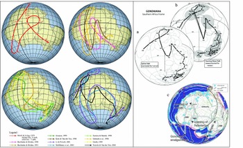
Since Creer, Irving & Runcorn (Reference Creer, Irving and Runcorn1954), palaeomagnetism has been used to track the movement of crustal elements. Although the amount of data has become impressive over the years (see the IAGA palaeomagnetic database: http://www.ngdc.noaa.gov/geomag/paleo.shtml), the spatial coverage is not uniform, the temporal coverage decreases strongly back into the past, and the accuracy has always been the subject of intense debate. The concept of filtering data has been a critical point of using palaeomagnetic data for the reconstructions. With the same dataset, the way data are filtered can lead to very different apparent polar wander paths (APWP; e.g. C. Vérard, unpub. Ph.D. thesis, Univ. Munich (LMU), 2004). For example, a landmass as important as Gondwana has long been the subject of very large uncertainties (Fig. 4), although Domeier, Van der Voo & Torsvik (Reference Domeier, Van der Voo and Torsvik2012) recently proposed ways to reconcile different points of view. The APWP of Torsvik et al. (Reference Torsvik, Müller, Van der Voo, Steinberger and Gaina2008, Reference Torsvik, Van der Voo, Preeden, Mac Niocaill, Steinberger, Doubrovine, van Hinsbergen, Domeier, Gaina, Tohver, Meert, McCausland and Cocks2012), with a relatively short Silurian–Devonian loop, now seems fairly widely accepted even if Stampfli et al. (Reference Stampfli, Hochard, Vérard, Wilhem and von Raumer2013), for instance, still questioned their late Proterozoic – Early Palaeozoic segment.
Left panel: Apparent polar wander paths (APWP) for Gondwana for Palaeozoic times as shown in C. Vérard (unpub. Ph.D. thesis, Univ. Munich (LMU), 2004, fig. 2-1 and references therein). In the mid-2000s, two schools of thought were still active in the community of palaeomagneticians according to the chosen filter for the data: as highlighted by Morel & Irving (Reference Morel and Irving1978), some favoured a relatively straightforward path – of X-type – through Gondwana, while others proposed a path – of Y-type – with a big loop passing south of South America and involving very high speeds for Gondwana. Right panel: Current APWP for Gondwana now largely favour paths with short loops; (a, b) APWP after Torsvik et al. (Reference Torsvik, Van der Voo, Preeden, Mac Niocaill, Steinberger, Doubrovine, van Hinsbergen, Domeier, Gaina, Tohver, Meert, McCausland and Cocks2012, fig. 11); (c) after Stampfli et al. (Reference Stampfli, Hochard, Vérard, Wilhem and von Raumer2013, fig. 5; © Neftex, v.2010).

If palaeomagnetic data constrain the positions of crustal elements in latitude and rotation relative to north, they do not provide information on the longitudinal movements. Efforts have thus been made to overcome this issue in particular using hotspots (e.g. Müller, Royer & Lawver, Reference Müller, Royer and Lawver1993; Courtillot et al. Reference Courtillot, Davaille, Besse and Stock2003; Torsvik et al. Reference Torsvik, Müller, Van der Voo, Steinberger and Gaina2008, Reference Torsvik, Steinberger, Gurnis and Gaina2010; Wessel & Kroenke, Reference Wessel and Kroenke2009). However, the reference to hotspots only allows going back to the Cretaceous, although Torsvik et al. (Reference Torsvik, Müller, Van der Voo, Steinberger and Gaina2008) were able to extend their ‘Global Hybrid Reference Frame’ back to 300 Ma.
Following Morley (rejected paper, 1963) and Vine & Matthews (Reference Vine and Matthews1963), the magnetic anomalies of the ocean floor are interpreted as markers of spreading. Royer et al. (Reference Royer, Müller, Gahagan, Lawver, Mayes, Nürnberg and Sclater1992) – updated by Müller et al. (Reference Müller, Roest, Royer, Gahagan and Sclater1996, Reference Müller, Roest, Royer, Gahagan and Sclater1997, Reference Müller, Sdrolias, Gaina and Roest2008) and reviewed by Seton et al. (Reference Seton, Whittaker, Wessel, Müller, DeMets, Merkouriev, Cande, Gaina, Eagles, Granot, Stock, Wright and Williams2014) – defined a list of magnetic anomaly identifications, and produced Euler poles used in almost all models of reconstructions. However, c. 60% of the lithosphere has been subducted since 150 Ma and is therefore missing nowadays (Torsvik et al. Reference Torsvik, Steinberger, Gurnis and Gaina2010). Thus, for the major plates (i.e. African plate, South American plate, etc.), differences between the models are minor, and only have an impact at high spatial and/or time resolutions. However, some oceanic areas (circum-Antarctic, West Pacific, West Australia, etc.) are still the subject of strong debate.
The similarities in the shapes of coastlines were the first clues used to suggest that the continents have moved relative to each other. Nevertheless, it is Bullard, Everett & Smith (Reference Bullard, Everett and Smith1965) who first proposed the reconstruction of Pangaea with a quantitative approach for a best-fit between continents. However, the method does not take passive margin stretching into account. Great progress could nevertheless be made by creating a 3D restoration project of passive margins on a global scale as De Melo Garcia (Reference De Melo Garcia2012) did at the local scale for instance. It would be useful to have an accurate and detailed picture of the position and relationships between continental blocks at least at the time of Pangaea.
Other data are widely used to create reconstructions.
(1) Dating data (palaeontological or geochemical), although central to the reconstruction and quantitative in nature, can precisely fix events in time, but not spatially.
(2) Gravity data also, for instance, provide first-order information for the definition of limits upon the current configuration of the Earth, such as, in particular, the definition of Continent–Ocean Boundaries (COB) at the foot of passive margins, for example. As for the definition of isochrons, COB definition can be considered as data allowing for a quantitative fit. However, the definition of COB remains subject to debate. In the UNIL model, for example, a COB is defined as the boundary marking the end of the separation between two adjacent continents after rifting; the area between them is termed ‘oceanized’, regardless of the type of sea-floor present: oceanic crust, mantle or even ‘continental allochthons’ (Manatschal & Müntener, Reference Manatschal and Müntener2009), i.e. chips of continent ‘lost’ during oceanization. Others (e.g. Manatschal & Müntener, Reference Manatschal and Müntener2009; Direen et al. Reference Direen, Stagg, Symonds, Norton, Mohriak, Danforth, Post, Brown, Tari, Nemčok and Sinha2012) distinguished the ‘thinned continental crust’ (i.e. the necking zone), then the ‘Continent–Ocean Transition Zone’ (COTZ) and finally the COB (sensu stricto), which marks the transition towards the establishment of an oceanic crust. Note, however, that extension – and thus thinning – is not necessarily restricted to the necking zone and usually extends well beyond on the mainland. The COTZ has internally complex aspects, ‘which shows features in common with magma-poor rifted margins worldwide, such as basement ridges interpreted as exhumed subcontinental mantle’ (Direen et al. Reference Direen, Stagg, Symonds, Norton, Mohriak, Danforth, Post, Brown, Tari, Nemčok and Sinha2012). When present as remnants in a suture zone for instance, it is therefore very difficult to distinguish the COTZ from denuded mantle near slow spreading mid-oceanic ridges (amagmatic ridges and ‘oceanic core complex’) as in the current Indian Ocean (e.g. Baines et al. Reference Baines, Cheadle, John and Schwartz2008; Kamesh Raju et al. Reference Kamesh Raju, Samudrala, Drolia, Amarnath, Ramachandran and Mudholkar2012), in the Arctic Ocean (e.g. Dick, Lin & Schouten, Reference Dick, Lin and Schouten2003; Michael et al. Reference Michael, Langmuir, Dick, Snow, Goldstein, Graham, Lehnert, Kurras, Jokat, Muhe and Edmonds2003) or along the Cocos-Nazca spreading centre, for example (Fryer, Reference Fryer2002; see also Püthe & Gerya, Reference Püthe and Gerya2014). These distinctions, while important, are thus difficult to apply to reconstructions of the past.
3.b.1.b. Semi-quantitative data
The semi-quantitative data are critical even though they often yield solutions far from unique. They consist primarily of definitions and correlations of lithofacies, and biostratigraphic definitions and correlations where possible. They are largely augmented by geochemical data characterizing the source rocks (e.g. zircons). These geochemical data, although quantitative by nature, can only provide information on the relative spatial and temporal localization.
Nevertheless, these data allow us to reconstruct two types of environments:
(1) The biogeographic and palaeoclimatic environments: Although Suess (Reference Suess1892) used the distribution of Glossopteris fossils (Brongniart, Reference Brongniart1828) in particular to consider a connection between different parts of Gondwana, Wegener (Reference Wegener1912) was the first to propose a map of Pangaea based on this type of data. Since the advent of plate tectonics, Hughes (Reference Hughes1973) and then Cocks & Fortey (Reference Cocks and Fortey1982) were the first to define (regional) maps after the distribution of fossils and their living environment, and many reconstructions now incorporate this type of data. However, before a fossil plant or animal can be used for palaeogeographic purposes, both its age and its own ecology must be assessed correctly. Such work is very delicate since it requires significant assumptions often based on or derived from present-day observations. Detailed ecology of conodonts for example remains an issue. Since their dispersal and evolution are rapid, the use of their fossils as biogeographic indicators must be regarded with caution. In addition, one must note that, in general, biodiversity is greater closer to the equator than at high latitudes, giving unequal uncertainties for the palaeogeographies.
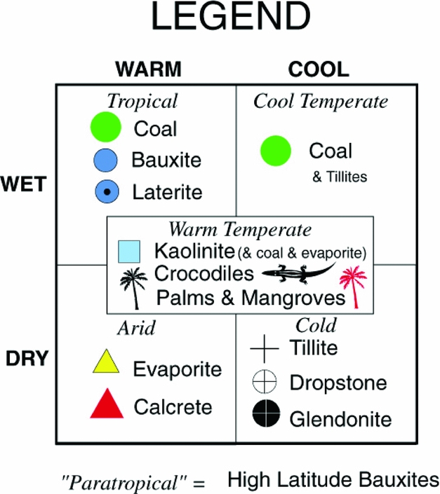
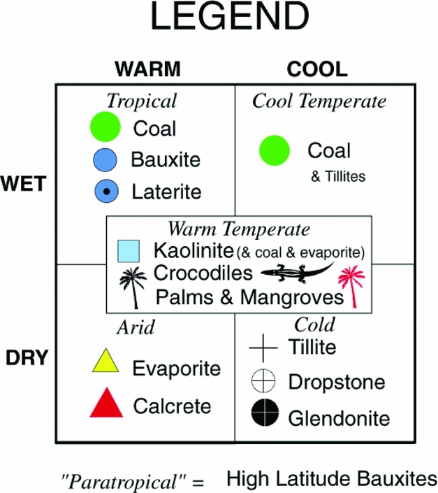
The palaeoclimatic indicators are also widely used. The PaleoMap Project, for example, has maps of climatic zones based on the distribution of ‘lithologic indicators of climate’, namely the distribution of coal, bauxite, laterite, evaporite, calcrete, tillites, dropstones, glendonite and kaolinite (Fig. 5; see Boucot et al. Reference Boucot, Xu, Scotese and Morley2013). These data are very important and include the ability to validate or invalidate some hypotheses; however, their accuracy remains relative on the one hand, and these data should be considered collectively on the other hand, because they can be subject to significant local effects. Nowadays, for example, the Clinton Lake in Canada is associated with evaporites (e.g. Renaut, Reference Renaut and Rosen1994) while the lake is located in the boreal region. Thus, while it is true that globally, evaporites can readily form in the hot and arid subtropical belt (see Fig. 5), evaporites are in fact just the result of the local water balance (see also the Messinian Crisis).
Legend provided by Christopher Scotese (http://www.scotese.com/legend.htm; see also Boucot et al. Reference Boucot, Xu, Scotese and Morley2013) for the ‘palaeoclimatic reconstructions’ of the PaleoMap Project.
(2) The geodynamic environments: The following geodynamic environments can often be well characterized in the field: rift zones (typically from syn-rift sedimentation), passive margins (post-rift sedimentation related to thermal subsidence), active margins (i.e. cordillera; from intra-continental arc magmatism and high-pressure metamorphism), intraoceanic subduction zones (oceanic arc magmatism and metamorphism), obduction zones (ophiolitic sequence and low-pressure metamorphism), collision zones (metamorphism, flysch and molasse). To the list can be added the often well-identified areas of intraplate volcanism (hotspot, traps), which can be seen as a zero-valued geodynamic environment (i.e. not related to geodynamics). From those data, not only associations or exclusions between various ‘puzzle pieces’ can be made, but also information on the geodynamic setting can be retrieved. Associated within a plate, those geodynamic environments must be coherent with all the forces acting at the plate boundaries. The identification of those environments within each ‘puzzle piece’ is therefore key for constraining their position among other pieces.
The UNIL and Panalesis models are particularly built around these notions of geodynamic environments.
It should be noted that structural data are also sometimes put forward to constrain reconstructions. This is the case for the alignment of Mesoproterozoic mountain chains for the Columbia supercontinent (Rogers & Santosh, Reference Rogers and Santosh2002; see also Rogers & Santosh, Reference Rogers and Santosh2003) or Grenvillian mountain chains for Rodinia (McMenamin & McMenamin, Reference McMenamin and McMenamin1990; Hoffman, Reference Hoffman1991) for example, or for correspondence of fractures within Pangaea (M. Moulin, unpub. Ph.D. thesis, Univ. Western Brittany, 2003; Moulin, Aslanian & Unternehr, Reference Moulin, Aslanian and Unternehr2010). However, the (non-)linearity of the original system and the accuracy of the definition of the structures (usually drawn as a line on the global scale map but consisting of a broad deformed zone in the field) make this type of work hard, and the results are often tainted with strong uncertainties.
3.b.1.c. Synthetic data
According to the ‘dynamic plate boundary approach’ (Stampfli & Borel, Reference Stampfli and Borel2002; and see the Methods Section 3.b.2 below), the UNIL model is the only published model to clearly and systematically rely on synthetic data that strongly constrain the model in terms of geometry and kinematics.
However, Müller et al. (Reference Müller, Roest, Royer, Gahagan and Sclater1997, Reference Müller, Sdrolias, Gaina and Roest2008) and Seton et al. (Reference Seton, Müller, Zahirovic, Gaina, Torsvik, Shephard, Talsma, Gurnis, Turner, Maus and Chandler2012) have, in their isochrons dataset, synthetic isochrons, such as isochrons proposed in the Mediterranean Sea. Although the reason for including them in their dataset and how these isochrons were obtained is not really explicit, some are just the result of the method used to define the isochrons. The use of the Hellinger code (Hellinger, Reference Hellinger1981), indeed, implies defining pairs of magnetic anomalies; if an anomaly is present on one plate, a second, exactly the same, will be generated on the other plate (see chrons C18 (~ 40 Ma) and C21 (~ 48 Ma) on the Nazca plate after Müller et al. Reference Müller, Roest, Royer, Gahagan and Sclater1997).
Finally, Gurnis et al. (Reference Gurnis, Turner, Zahirovic, DiCaprio, Spasojevic, Müller, Boyden, Seton, Constantin Manea and Bower2012) has recently introduced the concept of a ‘continuously closing plate’. Although the method is well defined, its use to constrain the reconstructions remains to be further clarified. Thus, the definition of the plates and their geometric, kinematic and/or geodynamic use as done by Domeier & Torsvik (Reference Domeier and Torsvik2014), in particular, will certainly need to provide further information in the future.
3.b.2. Methods
3.b.2.a. ‘Puzzle pieces’
All models first define a division of the crust into ‘puzzle pieces’ (Fig. 6). These elements are defined on the basis of geological maps and represent elements of the Earth's crust that have suffered the same story – the same movements at the scale of the globe – over the period that the reconstructions consider.
Three examples of division of the crust into ‘puzzle pieces’: (a) according to Seton et al. (Reference Seton, Müller, Zahirovic, Gaina, Torsvik, Shephard, Talsma, Gurnis, Turner, Maus and Chandler2012) who used the EarthByte model; (b) according to the PLATES project; (c) after Vérard et al. (Reference Vérard, Hochard, Baumgartner and Stampfli2015a, fig. 1) for the UNIL model (© Neftex; v.2010).

For example, Seton et al. (Reference Seton, Müller, Zahirovic, Gaina, Torsvik, Shephard, Talsma, Gurnis, Turner, Maus and Chandler2012) used 202 continental ‘puzzle pieces’ (in grey in Fig. 6, augmented by 1374 polygons associated with isochrons in colour as a function of age in Fig. 6) for their reconstructions between 200 Ma and 000 Ma, while Domeier & Torsvik (Reference Domeier and Torsvik2014) used, with the same EarthByte model but for reconstructions between 410 Ma and 250 Ma, 972 ‘puzzle pieces’ (see ftp://ftp.earthbyte.org/earthbyte/GPlates/SampleData/FeatureCollections/Rotations/Global_EarthByte_PlateIDs_20071218.pdf). By comparison, the UNIL model used 1046 ‘puzzle pieces’ for reconstructions over 600 Ma, and the basic PLATES project used 377 ‘puzzle pieces’ for reconstructions over 750 Ma (Fig. 6; a high-resolution version has over 1200 pieces according to C. Scotese, pers. com. 2017).
Of course, this division is highly dependent on the spatial and temporal resolution of the model. Locally, nappes or tilted blocks can have very different movements relative to the whole of the ‘puzzle piece’. This also poses a problem for models that do not incorporate different types of data. For models exclusively based on palaeomagnetic data in particular, recorded motions may reflect local motions significantly different from the rest to the ‘puzzle piece’, and therefore in apparent contradiction with it. Ideally, such types of problems should be solved by a much finer division and/or much more dense coverage of palaeomagnetic data at all ages. For the moment, it seems that the best way to overcome this issue is to compile a set of data from various sources (quantitative, semi-quantitative and even synthetic) for each ‘puzzle piece’, and not to be too strict regarding the representation of a given datum relative to the entire set of data.
The term ‘puzzle piece’ is used here because it really reflects the will of all models to have a division of the present-day world, which then allows placing these elements in their genuine configurations in the past. The term is also selected because it is neutral with respect to the number of terms that have been used for reconstructions. The EarthByte model uses for example the term ‘plates’. This term is unfortunate because it obviously carries confusion with the concept of plate tectonics. Many models use the term ‘terranes’, but it is also regularly disputed because it refers to the definition of ‘a fault bounded package of rocks of regional extent’ proposed by Howell, Jones & Schermer (Reference Howell, Jones and Schermer1985), a definition that does not usually correspond to the division done for the models. In addition, the term ‘terranes’ was used long before the advent of plate tectonics (d'Aubuisson de Voisins, Reference D'Aubuisson de Voisins1828; Schardt, Reference Schardt1893; Dana, Reference Dana1880) and its fundamental meaning has been a matter of hot debate (e.g. Sengör, Dewey & Robertson, Reference Sengör, Dewey and Robertson1990; Howell, Reference Howell1995; Le Grand, Reference Le Grand and Oldroyd2002). It is the same with the words ‘blocks’ or ‘microcontinents’ among others. Therefore, Hochard, Vérard & Baumgartner (Reference Hochard, Vérard and Baumgartner2011) and then Vérard et al. (Reference Vérard, Hochard, Baumgartner and Stampfli2015a) have chosen to introduce the term ‘geodynamic units’ (GDUs) for the UNIL model (the term was actually used as early as 2009 in K. Flores-Reyes, unpub. Ph.D. thesis, Univ. Lausanne, 2009). Owing to legal issues regarding the UNIL model (now the property of Neftex) and given that the link between some concepts of geodynamics and the division made for the reconstructions is questioned by some, the upcoming Panalesis model shall use the term ‘tectonic elements’, which simply refers to a part of the Earth's crust, without prejudice towards either its nature, continental or oceanic, or its internal deformations (presence of nappes, tilted blocks, (mega-)kinking, etc.). The term refers back to the ‘tectonic elements’ formerly used by Ross & Scotese (Reference Ross and Scotese1988).
3.b.2.b. ‘Single control’ versus ‘dual control’ approaches
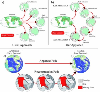
The data, mapped on the present-day world, are then transferred back into the past using the ‘puzzle pieces’ and finite-rotation poles to create a reconstruction at a given age. To constrain this reconstruction, two methods are used: the ‘single control’ approach and the ‘dual control’ approach (Vérard et al. Reference Vérard, Hochard, Baumgartner and Stampfli2015a; Fig. 7).
Upper panel: (a) ‘Single control’ approach; geological data (s.l., quantitative and/or semi-quantitative) are mapped on the present-day configuration and transferred back in time to the considered time slice to be reconstructed. (b) ‘Dual control’ approach; geological data (s.l.) from the present-day are used to reconstruct ‘key assemblies’ in the past; from those key assemblies, geodynamic scenarios are generated from one time slice to another, and geological data (s.l.) from the present day are used to confirm or refute the proposed reconstruction path in between the two key assemblies. Lower panel: The resulting reconstructions (c) and (d) do not reflect the iterative method of the reconstruction path in between the two time slices, although many hypotheses were tested. After C. Hochard (unpub. Ph.D. thesis, Univ. Lausanne, 2008) and Vérard et al. (Reference Vérard, Hochard, Baumgartner and Stampfli2015a, fig. 4) for the UNIL model (© Neftex; v.2010).
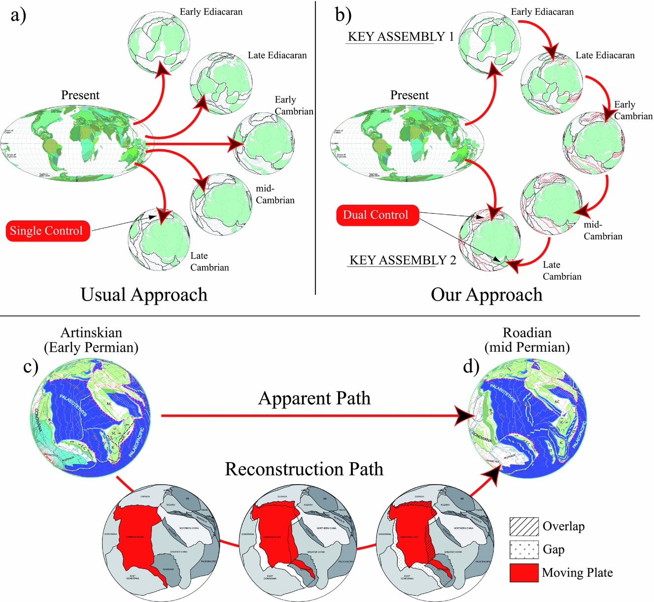
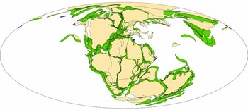
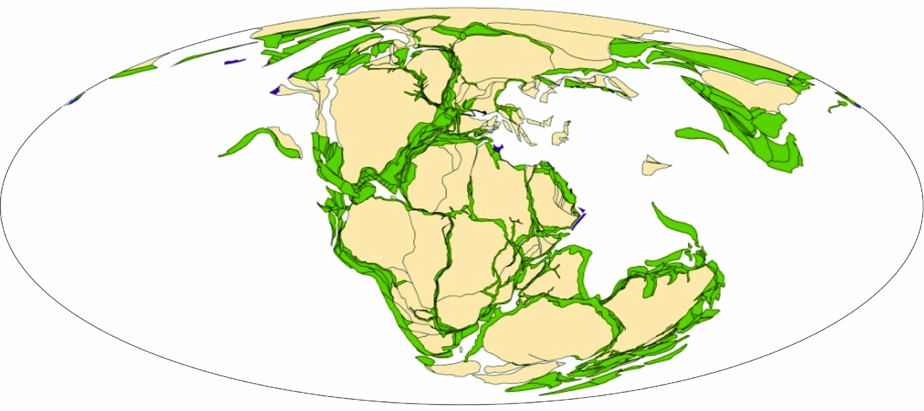
Many models proceed from the ‘single control’ approach: all data for a given age, e.g. all data Early Jurassic in age, say ~200 Ma, are used to define palaeo-positions and/or palaeogeographies for that age (e.g. Fig. 8). This method needs to have data all around the world for each age considered. Not only is that never the case, but if ‘puzzle pieces’ have their position constrained each by a single datum, it is very difficult to assess the quality of the reconstructed area, in particular if the palaeo-position has questionable implications.
Global reconstruction at 200 Ma after the Plate Wizard™ model (image courtesy of CGG Roberston), former version of the Robertson's Plate Kinematics model. The model focuses on the drift of continental ‘puzzle pieces’ and no tectonic plates are shown (the oceans, in particular, are empty of any plate tectonic boundaries). A great job, however, has been carried out to create a ‘deformable model’, i.e. to take into account the quantification of extension and shortening associated with the ‘puzzle pieces’.
With the ‘dual control’ approach, the idea is to use data compilations for ‘key assemblies’ (Vérard et al. Reference Vérard, Hochard, Baumgartner and Stampfli2015a; Fig. 7), i.e. key places and key moments for which a relatively high number of data exist. This may be the case, for example, for the break-up of a continental ribbon from a first continent – well-constrained by the rifting phase (syn-rift sedimentation, magmatism) and then the phase of oceanization (subsidence curve, post-rift sedimentation, remnant of ophiolitic sequence) – and then by the arrival of this continental ribbon in collision with a second continent (metamorphism, syn-collisional sedimentation, syn- and post-collisional magmatism, etc.). Between these two ‘key assemblies’, the palaeo-positions are constrained both by the existing data at the given age (transferred from the present day to the past as is the case for the ‘single control’ approach), and by the movement of the entire tectonic plate, which is done in agreement with a geodynamic scenario imagined in 3D. The plate rotation in the example of Figure 7c, d may be first inferred from data for the rifting of the Cimmerian Blocks transferred back to the Early Permian period by the ‘single control approach’. But the resulting stage pole concerns not only the continental elements included in the Cimmerian Blocks, but the entire tectonic plate shown in red. The second control consists therefore in checking whether the proposed movement of the (red) plate is geologically consistent with all available data all around the plate boundaries, geometrically consistent at all plate boundaries, kinematically consistent and in particular whether the plate speed at any point location on the plate (even the furthest) is not totally unrealistic, and geodynamically consistent, i.e. in agreement in particular with the forces acting at plate boundaries.
This ‘dual control’ approach is therefore highly iterative, because the movement (and stage pole) of the whole of the tectonic plate must be reset if the data constraining positions between two ‘key assemblies’ are not in accordance with the movement determined a priori. Moreover, this approach is also predictive inasmuch as the proposed movement of the whole tectonic plate implies effects which are likely to be observed in the geological record in other locations on the plate. Consequently, the model can be used to focus the search for information in the field or in the literature for well-circumscribed areas. However, this iterative work by trial and error – this path reconstruction (Fig. 7) – does not show up in the set of maps ultimately released. This lack of information about the reconstruction process may be a difficulty for readers but it is almost impossible for map authors to display the large number of tested variants for each reconstructed time slice. It is also important to understand that a list of Euler poles is not sufficient to define a plate tectonic model, since Euler poles alone do not define the position and shape of plate boundaries.
3.b.2.c. Plate boundary definition
As stated in Section 1, what makes a plate tectonic model are the plates, and in particular, the plate boundaries. To date, the UNIL model is the only published model to have been designed with closed tectonic plates covering 100% of the planet for all reconstructed ages throughout the Phanerozoic, i.e. even at times when isochrons no longer exist. Recently, however, the EarthByte model incorporated complete definitions of tectonic plates even for the Palaeozoic (Domeier & Torsvik, Reference Domeier and Torsvik2014).
Most other models have focused on the position of the continents, which drift on the surface of the globe; no plate or plate boundary appears to be considered as one can see from the Plate Wizard™ model for example (Fig. 8).
Since boundaries must be defined around the tectonic plates in order to create plate tectonic models, one must understand the behaviour of the lithospheric plates. Tectonic plates are commonly regarded as rigid bodies of the Earth's outer shell. However, the rigidity of the lithosphere has been questioned by some (e.g. Ribeiro, Reference Ribeiro2002) who argue for ‘soft plate tectonics’. It is true that some plate boundaries – intraoceanic arcs, collision areas, including areas of oroclinal bending formation – show that the plate boundaries are easily prone to large deformations.
Although powerful techniques have been developed to numerically model plate boundaries with high deformation and to help to refine reconstructions (e.g. Beaumont et al. Reference Beaumont, Jamieson, Nguyen and Medvedev2004; Jamieson et al. Reference Jamieson, Beaumont, Medvedev and Nguyen2004; Govers & Wortel, Reference Govers and Wortel2005; Huismans & Beaumont, Reference Huismans, Beaumont, Karner, Manatschal and Pinheiro2007; Smith et al. Reference Smith, Kurtz, Richards, Forster and Lister2007; Gerya, Reference Gerya2011; Kneller et al. Reference Kneller, Johnson, Karner, Einhorn and Queffelec2012; May, Schellart & Moresi, Reference May, Schellart and Moresi2013; Flament et al. Reference Flament, Gurnis, Williams, Seton, Skogseid, Heine and Müller2014; Püthe & Gerya, Reference Püthe and Gerya2014), no global reconstruction model uses those tools routinely for the following reasons: (1) it is a separate discipline that requires specific skills and time, often incompatible with the work required to create global reconstructions of the past; (2) the computational effort to model one given plate boundary is large; (3) the models are usually parameterized to fit to the studied cases, and it is therefore difficult to apply routinely to all plate boundaries of a global plate tectonic model. For now, when such models are used, it is essentially done a posteriori to validate certain geodynamic assumptions.
In global reconstructions models – and even if some make it their specificity (Plate Wizard™ model; and see Adriasola Munoz et al. Reference Adriasola Munoz, Harris, Glover, Goodrich, Hudson and Ady2010) – extensions and shortening at plate boundaries are most of the time simply taken into account by allowing overlaps or loose fits between the ‘puzzle pieces’ (e.g. the UNIL model; Vérard et al. Reference Vérard, Hochard, Baumgartner and Stampfli2015a).
3.b.2.d. The case of disappeared oceans
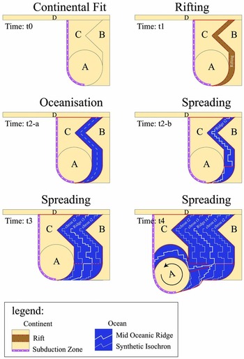
To create ridges and synthetic isochrons in disappeared oceans, Stampfli & Borel (Reference Stampfli and Borel2002) devised a simple but powerful method: the ‘dynamic plate boundary approach’ (Fig. 9), which can be summarized as follows.
Sketch showing the ‘dynamic plate boundary approach’ of Stampfli & Borel (Reference Stampfli and Borel2002), with, in particular, the definition of a synthetic ridge and isochrons in disappeared oceans. After Vérard et al. (Reference Vérard, Hochard, Baumgartner and Stampfli2015a, fig. 3).
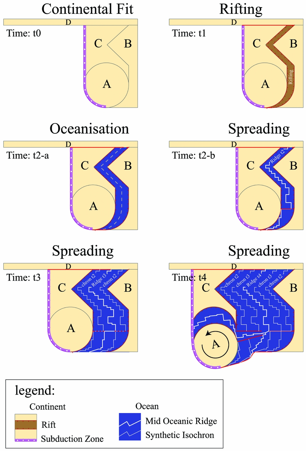
Insofar as is known that a continental fragment (e.g. continental ribbon) breaks off from a main continent according to the geological data (sensu lato, i.e. quantitative and/or semi-quantitative), it is possible to define a geodynamic scenario that begins with a rifting phase (time t1 in Fig. 9) and a phase of oceanization (time t2-a in Fig. 9). However, what matters in plate tectonics is less where the continent is located (‘puzzle pieces’ A & C in Fig. 9) but where and what the plate boundaries are. Yet, in the sketch at time t2-a (Fig. 9), the boundaries of the plate ‘AC’ correspond to two transform faults (top and bottom) and a subduction zone (left). Therefore, a plate boundary (right) is missing in the newly ‘oceanized’ area to close the plate: in this case, a mid-ocean ridge. What is the exact position of this ridge? What is its exact shape? It is impossible to say, now or ever, because the ocean has disappeared and might be exposed only as a suture in a mountain range. Nevertheless, the plate boundary necessarily had to exist, and should be located in the newly oceanized space. Subsequently, one can simply draw it, as is currently observed for mid-ocean ridges, i.e. with segments and transforms (time t2-b in Fig. 9).
This object is very important because it is thereafter used to create synthetic isochrons on each plate, namely the ‘AC’ plate (left) and ‘BD’ plate (right). These isochrons then define the space in which the new mid-oceanic ridge can be drawn (time t3 in Fig. 9). Thus, the ancient ocean is reconstructed step by step.
This method, although simple, is very powerful, especially when used on the sphere on a global scale (i.e. 100% of the surface is reconstructed). The slightest movement of a plate has implications which must be consistent with the global geological record (sensu lato) and consistent with the forces acting at plate boundaries (i.e. consistent with geodynamics). Furthermore, this method provides high constraints in terms of geometry and in terms of kinematics. In particular, if continent ‘A’ breaks up from ‘B’ (time t4 in Fig. 9), the rotation is greatly limited by the geometry at the triple junction and by the resulting spreading rate.
3.b.2.e. From one geodynamical environment to the other and constraints on plate tectonic models
In textbook examples of a Wilson Cycle, a continent breaks up by rifting, and oceanization then occurs between the two separated continents, until the configuration changes from a divergent regime to a convergent regime. Consequently, subduction initiates, leading to the closure of the ocean, and finally the two continents collide and reunite again.
The reconstruction method used (i.e. ‘single control’ or ‘dual control’ approach) has often no major impact on the first phase of the Wilson Cycle process (divergent regime; i.e. corresponding to Fig. 9). However, the change into a convergent regime (second phase) has great implications for the geodynamic configuration.
With models having no plate boundaries, continents can drift away one from the other or become closer without any apparent consequence when creating the reconstructions. When tectonic plates are considered, however, the possibilities to initiate a subduction zone are restricted to a few tectonic settings, which provide much higher constraints on the global reconstructions.
The case of oceanic ‘ridge failure’ has been proposed in various areas, such as onset of the New Caledonia Ophiolites for example (e.g. Lagabrielle et al. Reference Lagabrielle, Chauvet, Ulrich and Guillot2013). Nevertheless, the condition for ‘ridge failure’ or intraoceanic ‘transform fault failure’ to occur, relative to ‘passive margin reversal’ for instance (i.e. intraoceanic initiation versus initiation at the COB), is far from straightforward when generating reconstructions. If geological data are scarce or even absent, the choice to use one solution or the other may have great implications in terms of geodynamics.
On the contrary, the ‘spontaneous’ passive margin reversal (i.e. the change of a passive margin into an active margin) has proved to be highly unlikely (Cloetingh, Wortel & Vlaar, Reference Cloetingh, Wortel and Vlaar1989; Mueller & Phillips, Reference Mueller and Phillips1991; see also Cloos, Reference Cloos1993), because an oceanic lithosphere cannot break where it is the strongest. Passive margin reversal can therefore only occur after intraoceanic arc collision (Baes, Govers & Wortel, Reference Baes, Govers and Wortel2011), in the context of STEP faulting (Subduction-Transform Edge Propagator (STEP) after Govers & Wortel, Reference Govers and Wortel2005; see also the notion of subduction invasion as in Duarte et al. Reference Duarte, Rosas, Terrinha, Schellart, Boutelier, Gutscher and Ribeiro2013), or by ‘subduction propagation’ where subduction ‘jumps’ (or potentially propagates through detachment; Bartol & Govers, Reference Bartol and Govers2014) after collision of a continental fragment because the tectonic plate is kept pulled elsewhere. A ‘full’ plate tectonic model thus prevents the closure of an ocean such as the modern Atlantic Ocean without invoking one of the aforementioned contexts. This is a key aspect to take into account for proposing reconstructions for the future of the Earth.
On the other hand, when a subduction zone has initiated somewhere, there is no reason to stop it except in three cases: (1) obviously, in the case of collision with a passive margin, although it often leads to the initiation of a new subduction zone; (2) in the case of ‘collision’ with a spreading axis ridge, as was the case in Cenozoic time between the oceanic ridge of the Phoenix plate and the western border of the Antarctica plate; (3) in the case of collision with an oceanic plateau, such as the collision of the Hikurangi Plateau with the Chatham Rise. It is here worth mentioning that, although not observed in the present-day world, it is likely that the case of intraoceanic arc–arc collisions occurred in the geological past (see several cases proposed in Vérard & Stampfli, Reference Vérard and Stampfli2013a,b, for instance), but the resulting configuration is rather obscure, and at least, has never been tested numerically.
In summary, therefore, the definition of tectonic plates implies defining geodynamic settings at plate boundaries, which have implications not only at the chosen time slice, but also from time to time for the evolution of the system. Models accounting only for the position of continents thus disregard many constraints.
Now, some questions about potential constraints remain open, among which are:
(1) Does plate motion necessarily tend to align perpendicular to mid-oceanic ridges and trenches (and parallel to transform faults)? And if yes, is there a minimum size for this to happen? In the present-day world, there are clear examples, like the Nazca or Cocos ridges, where ridges are almost perpendicular to trenches. Conversely, the Java trench is near parallel to plate motion along the Andaman Arc. In our reconstructions, we have therefore not retained this criterion as a constraint for plate motion. However, statistical analysis over a long time period would be interesting, and numerical modelling might shed light on the subject.
(2) Are two ridge systems spreading side-by-side possible? The system has existed in the Scotia plate for instance around chron C5 (e.g. Vérard, Hochard & Stampfli, Reference Vérard, Hochard and Stampfli2012a and references therein) but it was a transient system just prior to ridge jump that formed the South Sandwich Island plate. In our reconstruction, we try to avoid this configuration although the underlying reasons remain obscure.
(3) Can island arcs cross ocean basins? The UNIL and Panalesis models at least, and the EarthByte models to some extent (see the ‘Cache Creek Oceanic plate’ in Matthews et al. Reference Matthews, Maloney, Zahirovic, Williams and Müller2016 for instance), strongly rely on the possibility for intraoceanic subduction zones to propagate across oceanic realms. We know it happened by roll-back processes for the Scotia and Caribbean arcs. These arcs are, however, relatively limited in width so that the mantle material can ‘easily’ move around the slab. What happens with larger slabs? Is the upper plate (and associated island arcs) motion then accommodated not by strict roll-back processes but by some subduction flattening? We argue in any cases that many passive margin environments cannot be turned into active margins (as seen in the geological record) if no arc–continent collision occurs. This requires island arc migration to be possible.
(4) Is there a speed limit for tectonic plates? Plate tectonic modellers ask this question to mantle convection modellers who return the question . . . Meert et al. (Reference Meert, van der Voo, Powell, Li, McElhinny, Chen and Symons1993), in particular, have already dealt with this question but the answer is not self-evident. In the UNIL and Panalesis models, an arbitrary speed limit is set at 25 cm.yr−1.
(5) Do tectonic plates move randomly over the planet? Vérard, Flores & Stampfli (Reference Vérard, Flores and Stampfli2012b) brought out some aspects about this. They showed that Euler poles are not randomly distributed over long time periods, although the data scattering suggests that tectonic plates predominantly live their own evolution. They also noticed that ‘tectonic plates with a large surface predominantly undergo translation (i.e. displacement along the great circle), whereas small plates show all ranges of motion, from spinning on themselves to translation’.
All those questions and more are part of ‘The 12 Rules of Plate Tectonics’ put together by Christopher Scotese (see Scotese, Reference Scotese2015), and collaborations between Earth surface and Earth interior modellers may provide answers to them.
4. Review of the main reconstruction types
The aim of this section is not to denigrate a particular model or praise another. It is clear that all have been immensely useful over the past decades. The goal is simply to put a finger on what works and what does not in the various models, to see if efforts could be combined to improve reconstructions, and to finally draw lines of research that could help to make advances in plate tectonic modelling.
4.a. Advantages and drawbacks of the different techniques
All global models have the same drawback: their spatial and temporal resolution is low. With a spatial resolution of c. 100 km (i.e. ~ 1°), coverage can be considered as excellent on a global scale, but an object such as Lake Geneva in Switzerland, for example, will not exist. This can lead to confusion with, for example, local geologists attached – rightly – to their field observations. If the models must be consistent with field data, models must also provide a framework to reposition local data in a more general context. On the other hand, for modeller(s) also, the danger lies in the approximations (required) made from local data, either by ignoring a given datum regarded as not representative of the general framework, or on the contrary, by extrapolating specific local data in terms of regional or global tectonics. It is possible therefore that these approximations lead to erroneous tectonic reconstructions. It is thus of benefit that several models co-exist and also that several solutions can be tested within a model.
Models built on the ‘single control approach’ have the advantage of being flexible. Theoretically, a single datum – especially palaeomagnetic – per ‘plate’ is necessary to determine a palaeo-position. The PLATES model or the reconstructions of Li et al. (Reference Li, Bogdanova, Collins, Davidson, De Waele, Ernst, Fitzsimons, Fuck, Gladkochub, Jacobs, Karlstrom, Lu, Natapov, Pease, Pisarevsky, Thrane and Vernikovsky2008), for example, go far back in the past, with reconstructions of supercontinents like Ur or Kenorland at ~3 Ga and ~2.5 Ga, respectively (Rogers & Santosh, Reference Rogers and Santosh2003). As Euler poles are defined from the present day to the past, stage poles can easily be defined between two reconstructions, and therefore by interpolating, reconstructions can be proposed at any age (e.g. Paleo-Continental Map Editor).
On the top of these reconstructions, many models also have the advantage of proposing further developments, such as drawing lithostratigraphic or palaeogeographic maps which look great (e.g. CPGeosystems model).
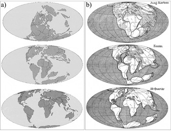
The problem of not showing plate boundaries can maintain the confusion – in particular for the general public – between continental drift and plate tectonics. By comparing reconstructions of Christopher Scotese (PaleoMap project, 1999), for example, with those of Alfred Wegener (Reference Wegener1929), the similarities to 70 years apart are striking (which is actually good; Fig. 10) but many people may think that the two theories are somehow synonymous when they are not.
Juxtaposition of maps derived from (a) an animation of Christopher Scotese (PaleoMap Project, 1999) and (b) maps after Alfred Wegener (Reference Wegener1929, fig. 4).

Models built on the ‘dual control approach’ have the advantage of being (theoretically) physically consistent, and take advantage of the wealth of the plate tectonic theory. Indeed, continuously evolving plate boundaries make the models geologically, geometrically, kinematically and geodynamically coherent.
On the other hand, they are relatively cumbersome to create, and the fact that one step constrains the next prevents – in the strict sense (i.e. by applying the ad hoc plate tectonic rules everywhere on the globe for each time slice) – the production of interpolated reconstructions at any age from the Euler poles (though Domeier & Torsvik, Reference Domeier and Torsvik2014 proposed to do so in their appendix; EarthByte model). In addition, these models are, at present, very focused on tectonics, and do not offer ‘beautiful maps’ as does Ronald Blakey (CPGeosystems maps) for example (but see the efforts made for the definition of palaeo-bathymetry and palaeo-hypsometry by the EarthByte Group and by Vérard et al. Reference Vérard, Hochard, Baumgartner and Stampfli2015b on top of the UNIL model). As a result, models generated with the ‘dual control’ approach method are, to date, far from being the most popular, especially in the media or in education.
Generally speaking, it must be stressed that a model of reconstruction of the Earth through the geological past cannot be reduced to a list of Euler poles. If such lists are useful for users of palaeo-maps (i.e. maps of reconstructions in the past) to locate their data in the genuine configuration (using ‘puzzle pieces’), Euler parameters must be the consequence of a model and not the source. If such confusion is made, the geodynamic constraints linked to tectonic plates – and in particular to their boundaries – are lost, and the resulting model cannot be properly named a plate tectonic model.
In addition, new avenues in plate tectonic modelling are undoubtedly linked to the coupling of global plate tectonic models with other global models for mantle convection, intraplate tectonic stresses, palaeotopography (bathymetry and hypsometry), palaeoclimate, vegetation and faunal evolution, erosion–sedimentation, geochemistry, etc. (see Section 6 on perspectives). The information required for such coupling is most often not contained in models built on the ‘single control approach’.
4.b. Uncertainty maps
One of the major issues of all models of plate tectonics lies in the fact that it is very difficult to produce uncertainty maps, and therefore objectively assess their relevance. The question does not only bear upon defining mathematical methods for drawing error ellipses around Euler poles in the presence of finite-rotation noise. Again, Euler poles do not define a plate tectonic model; rather they reflect its result. The question is to find a method for evaluating the match (or mismatch) between palaeogeographies generated by models and a series of data from a large number of disciplines of geosciences. Indeed, Euler poles are computed from topological objects (e.g. isochrons) but most of the reconstructions are based on affinities between different sets of data without any topology (e.g. lithofacies affinities).
In principle, determining uncertainty maps should be simple: it consists merely of using a colour (e.g. green) where the model is consistent with all the data, and another (e.g. red), where there is disagreement. But what uncertainty are we talking about?
Do we want to represent uncertainties between the data and the suggested geodynamic environments? For example, if arc magmatism data matches a subduction zone in the past, the agreement is good. However, note that the agreement will be ‘better’ if only one single arc magmatism datum coincides with a subduction zone, than if nine arc magmatism data and one hotspot magmatism datum are associated with a subduction zone, for example. Yet, one does not preclude the other.
Do we want to represent spatial uncertainty? The purpose of the reconstruction is to place data in their past configuration, and it is probably at this point that we would like to know the degree of uncertainty. If a rifting zone is drawn along the edge of a continent in the past, what degree of uncertainty will be assigned to a syn-rift sedimentation datum for example, defined in the present-day configuration, but found say 500 km south from where the rifting zone is proposed in the past? Clearly, the agreement is not very good. However, is this actually the shape of the rift zone that needs to be reviewed? Is it the Euler pole that allows the transfer of data from present to past that suffers from uncertainty? Is it also the age of the data that is poorly constrained, and with the movement of the plate, shifts the location of the data in the past? Is it all these things at once? And even, should the 500 km of offset be represented by a colour closer to green or closer to the red? In other words, what do we consider as a good spatial match?
For now, these issues have not been resolved. Although Müller et al. (Reference Müller, Sdrolias, Gaina and Roest2008) were able to provide an uncertainty map for their age grid of the ocean floor (topological objects with ages <180 Ma), no group, to date, has published uncertainty maps of their entire reconstructions.
While difficult, it should, however, be possible to define uncertainty maps assessing the quality of the reconstructions. Powerful correlation tools like convergent cross mapping (CCM; Sugihara et al. Reference Sugihara, May, Ye, Hsieh, Deyle, Fogarty and Munch2012) or information flow (IF; Schreiber, Reference Schreiber2000) have proved their efficiency and robustness and might be applied in this context.
5. Implications
Reconstructions of the Earth in the past are used, at least as general frameworks, in a large majority of studies in geosciences. The choice of a reconstruction model and its implicit concepts and assumptions, therefore, has broad implications.
5.a. Implications for the Earth's interior
The understanding of mantle dynamics, for example, requires the use of a plate tectonic model as the surface condition. In addition, a plate tectonic model provides data that can be compared with results from mantle flow modelling. A typical example of interplay between plate tectonic models and mantle flow modelling concerns the ‘engine’ of plate tectonics.
Forsyth & Uyeda (Reference Forsyth and Uyeda1975) examined the many forces acting on a given tectonic plate – namely asthenospheric driving and resistive drag forces, ridge push, slab pull, slab resistance (i.e. mantle resistance to the descending slab), colliding resistance (i.e. resistance of the lower plate to move past the upper one), transform fault resistance, suction (i.e. upper plate drawn by trench retreat) – and concluded that ‘slab pull’ is the main driving mechanism. The conclusion is, however, still debated. Doglioni et al. (Reference Doglioni, Carminati, Cuffaro and Scrocca2007), for instance, listed 22 counter-arguments against slab pull as the main driver, and favoured lithospheric net rotation – the westward drift – as the key parameter. There is, however, a broad agreement in the geodynamic community in favour of slab pull as the main force, and an extensive literature exists on net rotation and body forces (e.g. Ricard, Doglioni & Sabadini, Reference Ricard, Doglioni and Sabadini1991; Conrad & Lithgow-Bertelloni, Reference Conrad and Lithgow-Bertelloni2002; see also Vérard, Hochard & Stampfli, Reference Vérard, Hochard and Stampfli2012a for potential implications over the geological past).
Using a plate tectonic model, Vérard et al. (Reference Vérard, Hochard, Baumgartner and Stampfli2015a, fig. 10) have reported the mean tectonic plate velocities throughout the last 600 Ma. These authors confirmed in particular for the entire Phanerozoic the relationship found by Forsyth & Uyeda (Reference Forsyth and Uyeda1975) for the present-day world suggesting a correlation between the total length of subduction zones (i.e. global sum of trench lengths) and the mean tectonic plate velocities (Fig. 11a). They also confirmed that the amount of created areas (in km2.yr−1) is dominated by accreted areas at oceanic spreading ridges, and the amount of suppressed areas is dominated by consumed lithosphere at trenches (Fig. 11b). Such a relationship has led many authors to consider ‘slab pull’ and ‘ridge push’ as the main drivers of tectonic plates.
(a) Global feature length (km) per reconstruction using the UNIL model versus mean tectonic plate velocities throughout Phanerozoic time. (b) Global rates (km2.yr−1) per reconstruction using the UNIL model versus mean tectonic plate velocities throughout Phanerozoic time. Data after Vérard et al. (Reference Vérard, Hochard, Baumgartner and Stampfli2015a); general trend (linear fit) and 95% confidence interval (shaded areas) only shown to highlight the quality of the trend.
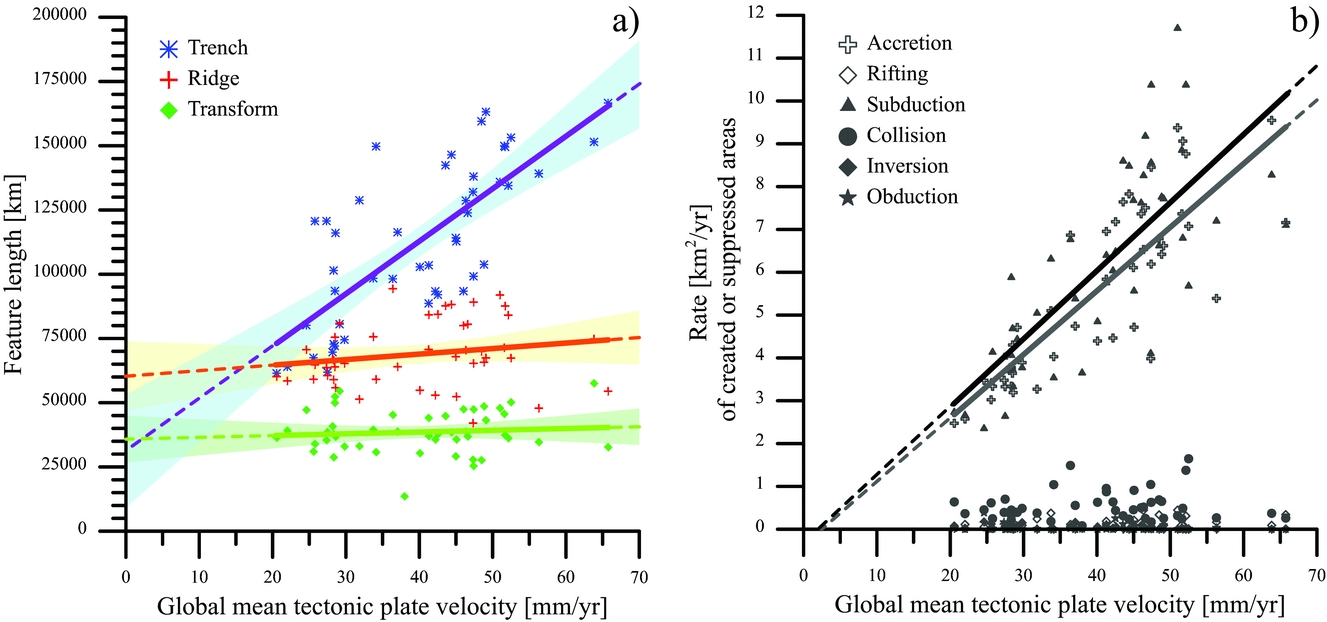
Between the two forces, it is clear that ‘slab pull’ is predominant over ‘ridge push’, proving that a mid-oceanic ridge is not at the centre of the system and should not be represented as such (section 2.c). In addition, the term ‘ridge push’ (which is nevertheless used here) is also relatively ambiguous because the plates actually exert a pull at oceanic ridges. It is evidenced by the African plate for example, which is limited to the east and west by mid-oceanic ridges, and is not under compression but in extension (e.g. World Stress Map, Heidbach et al. Reference Heidbach, Tingay, Barth, Reinecker, Kurfeß and Müller2009).
For the sake of clarity, avoiding sophisticated equations, the order of magnitude of ‘slab pull’ relative to ‘ridge push’ can be easily understood with a small simple (even simplistic) calculation as follows (Fig. 12a; see also Thomas, unpub. presentation, 2007 (in French): http://planet-terre.ens-lyon.fr/article/convection-PTho_conf.xml; Thomas, Reference Thomas2010):
(a) Schematic illustration (oversimplified) used for a simple calculation about the order of magnitude of ridge push relative to slab pull. Ridge push (PRP) is, in this configuration, ten times weaker than slab pull (PSP); see text. (b) Effect of eclogitization of oceanic crust during subduction; while the oceanic crust of density ρ = 2.9 acts as ‘float’ for the lithosphere, the crust turns into ‘ballast’ in subduction because of eclogitization. Modified after Thomas, unpub. presentation (2007) (in French): http://planet-terre.ens-lyon.fr/article/convection-PTho_conf.xml.

Consider a lithostatic pressure PB in B in Figure 12a – i.e. far from the ridge – where PB = ρB.g.h; PA in A – i.e. at the ridge – is PA = ρA.g.(h+Δh). Let's assume a density of the lithosphere ρB = 3300 kg.m−3, a density of the lithosphere ρA = 3250 kg.m−3, and a thickness of lithosphere ‘away from the ridge’, h = 100 km. According to the rules of isostasy, PA = PB. Thus, the relief at the ridge (compared to the ocean floor ‘away from the ridge’) is Δh ≈ 1.5 km.
Then, consider that ‘away from the ridge’ means a distance D = 1000 km, and the acceleration due to gravity is taken as g = 10 m.s−2. The angle α of the average slope between the top of the ridge and the bottom of the ocean floor ‘away from the ridge’ is α = arcsin(h/D) = arcsin(0.1) ≈ 5.74°. The force exerted on the triangular volume (shown by hatching in Fig. 12a) is F = h.L.g.(D/2).(ρB – ρA), with L the length of the mid-oceanic ridge (Fig. 12a). The force due to the ridge push is then FRP = F.sin(α), and ridge push corresponds to a pressure PRP = FRP/(h.L) = (D/2).g.(ρB – ρA).sin(α). With numerical values, PRP = 2.5×10⁷ N.m−2.
At the slab, assuming the dip is vertical over a depth Dpth = 500 km, the slab pull force is FSP = h.L.g.Dpth.(ρB – ρA). The pressure related to the slab pull is then PSP = FSP/(h.L) = g.Dpth.(ρB – ρA). With numerical values, PSP = 25×107 N.m−2.
Such a simple calculation shows that slab pull is approximately one order of magnitude higher than ridge push. Using more physically correct equations, Turcotte & Schubert (Reference Turcotte and Schubert2002) equally found a factor of 10, with 3.3×10¹³ N.m−1 for slab pull per unit length parallel to the trench (Turcotte & Schubert, Reference Turcotte and Schubert2002, p. 281), and 3.4×10¹² N.m−1 for ridge push (Turcotte & Schubert, Reference Turcotte and Schubert2002, p. 283).
In addition to those aspects, mineral phase transitions must be considered, one of which is key (and often not taken into account in ‘real’ numerical simulations, e.g. Wu et al. Reference Wu, Conrad, Heuret, Lithgow-Bertelloni and Lallemand2008; Davies et al. Reference Davies, Goes, Davies, Schubert, Bunge and Ritsema2012; Crameri et al. Reference Crameri, Tackley, Meilick, Gerya and Kaus2012; Bower, Gurnis & Flament, Reference Bower, Gurnis and Flament2015): the effect of eclogitization. Again, the impact of eclogitization can be easily understood with a simple sketch (Fig. 12b).
At the surface condition, a peridotite or mantle rock is commonly regarded as having a density of ρP ≈ 3.35 (e.g. 3.397 after Jordan, Reference Jordan1978). Below the lithosphere, i.e. beyond 1300–1350°C, the density of the asthenosphere is commonly taken as ρA ≈ 3.25, because ρA = ρP − Δρ = ρP − α.ρP.ΔT = 3.10−5×3.397×1350 = 3.259, where α is the coefficient of thermal expansion [K−1] and ΔT is the temperature difference [K] between the top and bottom of the lithosphere. Similarly, the mean density of the lithospheric mantle is ρLM ≈ 3.30, because ρLM = ρP − Δρ = ρP − α.ρP.(ΔT/2). The oceanic lithosphere, therefore, should not be buoyant on the asthenosphere if there was no oceanic crust (and/or serpentinized mantle), which has a density of ρC ≈ 2.8–2.9 (e.g. Attewell & Farmer, Reference Attewell and Farmer1976; Carlson & Raskin, Reference Carlson and Raskin1984). The crust thus has the role of ‘float’, until the thickness of the lithosphere becomes approximately eight to ten times the thickness of the crust (Fig. 12b). Assuming a typical oceanic crustal thickness of 6 km, a dimensionless temperature ratio θ = 0.1, and a thermal diffusivity κ = 0.727 mm2.s−1 in the calculation of the lithospheric thickness (Turcotte & Schubert, Reference Turcotte and Schubert2002, p. 155), the lithosphere becomes neutrally buoyant after c. 30 Ma (case no. 4 in Fig. 12b). Furthermore, while the slab should become more buoyant because it is re-heated during subduction, eclogitization has the opposite effect: the crust, which had the role of ‘float’ (density ρC ≈ 2.9), turns into ‘ballast’ (ρEC ≈ 3.4; case no. 5 in Fig. 12b).
Now, if slab pull is likely a key component on plate torques, it is clear that the link often made between the age of the sea-floor and the velocity of tectonic plates is far from trivial if any. Cruciani, Carminati & Doglioni (Reference Cruciani, Carminati and Doglioni2005) and Doglioni et al. (Reference Doglioni, Carminati, Cuffaro and Scrocca2007) have shown that no correlation can be drawn between convergence rates or slab dips and ages of the oceanic crust of the present-day world.
Plotting Vérard et al.’s (Reference Vérard, Hochard, Baumgartner and Stampfli2015a, fig. 10) data in a different way (Fig. 13), it appears that the aforementioned correlation is even negative over the Phanerozoic Eon. When the age of the oceanic crust is old at a global scale, plate velocities are low on average (Fig. 13a). The dispersion of crustal ages around the mean is not an issue, because when the dispersion (1σ) is high – meaning that the amount of sea-floor with ages much older or much younger than the mean is high – plate velocities are slower than when the dispersion is low (Fig. 13b), although the negative trend is hardly significant (at the 95% confidence level). The older areas of the sea-floor, therefore, do not seem to shift the mean values towards higher velocities.
(a) Global mean ages of the sea-floor per reconstruction using the UNIL model versus mean tectonic plate velocities, from 550 Ma to 000 Ma. (b) Dispersion of ages around the mean values provided in (a). (c) Global mean ages of the sea-floor entering subduction (i.e. ages at trenches). (d) Dispersion of ages at trenches around the mean provided in (c). Data after Vérard et al. (Reference Vérard, Hochard, Baumgartner and Stampfli2015a); general trend in red (linear fit) and 95% confidence interval in yellow only shown to highlight the quality of the trend.
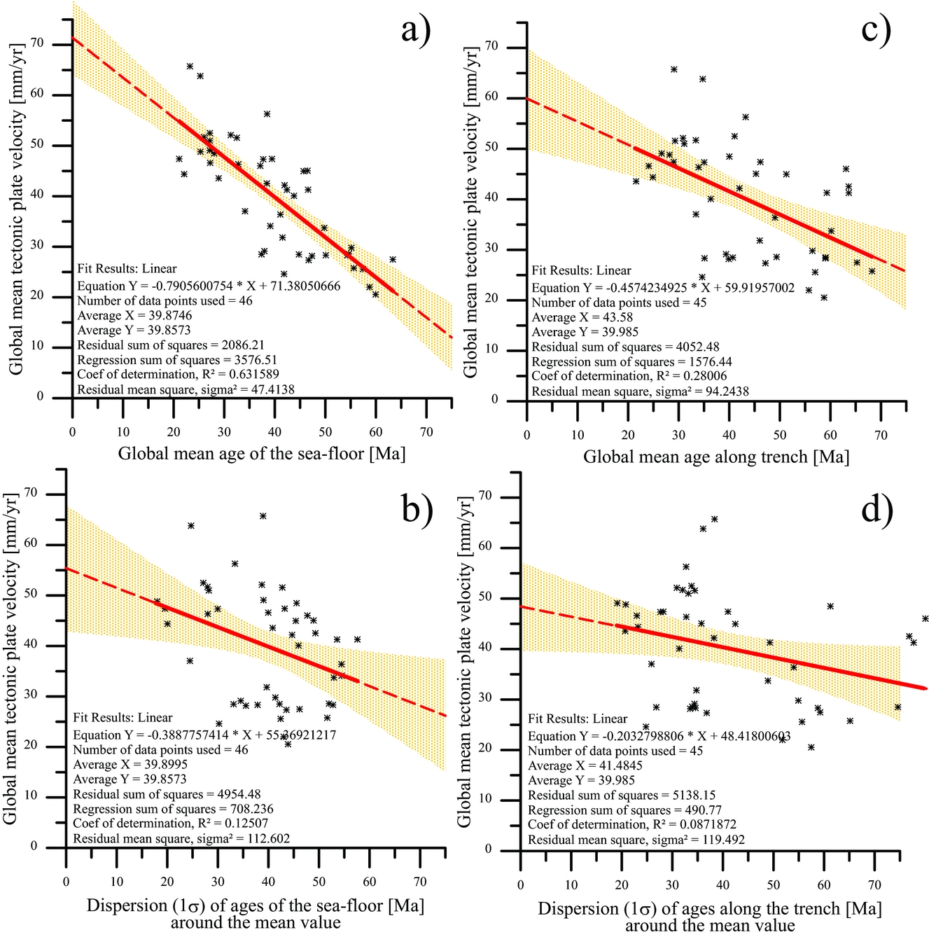
The result seems to hold when ages are not considered as the global mean but when only ages of oceanic crust entering subduction (i.e. ages at trenches) are taken into account (Fig. 13c, d).
At first glance, plate velocities therefore seem to be more related to the activity of the planet's interior than related to the state of the lithosphere. However, one must be cautious with such results (Figs 11, 13) because many factors may actually have an effect. The best way of assessing the role of the various forces on driving tectonic plates most probably corresponds to the approach carried out by Warners-Ruckstuhl, Govers & Wortel (Reference Warners-Ruckstuhl, Govers and Wortel2012). The latter authors retrieved the mechanical equilibrium for the Eurasian plate by combining lithospheric edge and body forces with mantle dynamics (Fig. 14). They showed that edge forces are the dominant contribution driving the Eurasian plate.
Relative magnitudes of mantle shear, lithospheric body force (LBF) and lithospheric edge force torques for balancing forcing models (zero net torque), expressed as a percentage of their scalar sum, and according to various mantle flow models. After Warners-Ruckstuhl, Govers & Wortel (Reference Warners-Ruckstuhl, Govers and Wortel2012, fig. 15).
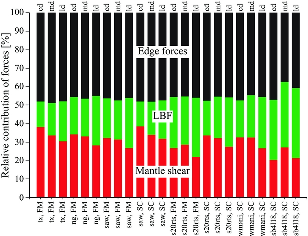
In order to answer the fundamental question of what drives plate tectonics, such excellent work shall be extended in space, over all the tectonic plates of the Earth, and also in time, through geological times using an appropriate plate tectonic model. The coupling between a lithospheric mechanical model and plate tectonic model is certainly the future of the discipline. Although those aspects are usually separated from palaeogeographic concerns, they are actually key in studying palaeogeographies. Vérard et al. (Reference Vérard, Hochard, Baumgartner and Stampfli2015b), for instance, showed that the effects of global plate velocities on large-scale variations of the sea-level, slab pull or slab detachment have a huge impact on the surface topography (e.g. Duretz & Gerya, Reference Duretz and Gerya2013) and dynamic topography (i.e. topography related to mantle convection), and might affect surface altitude by up to ± 1000 m (Davies, pers. com. 2010; see Čadek & Fleitout, Reference Čadek and Fleitout2003 or Shephard et al. Reference Shephard, Liu, Müller and Gurnis2012 for some examples of the large literature on the subject).
5.b. Implications for the Earth's exterior
Palaeogeographies (and palaeoenvironments) are the results of the combination of numerous factors. A correct plate tectonic model is the necessary framework to study palaeogeography but does not define it itself. The step from a plate tectonic model to a palaeogeographic model is very delicate to achieve. If a plate tectonic model positions the landmasses and defines the geodynamic environments through time, the palaeogeographies are first defined by the association of the topography and the sea-level, on top of which climate (i.e. ocean–atmosphere–cryosphere), hydrography and biosphere further define palaeoenvironments.
The choice of a reconstruction model therefore has implications for the understanding of external geodynamics. A typical example of such an issue is the study of climate in deep time.
In order to study the Early Toarcian climate for instance (Fig. 15), Dera & Donnadieu (Reference Dera and Donnadieu2012) used the palaeogeography map proposed by Blakey (Reference Blakey, Fielding, Frank and Isbell2008; CPGeosystems model). While the CPGeosystems model proposes beautiful maps with realistic-looking morphology, the topography is qualitative only and no altitude is provided. As done by most others (e.g. Sellwood & Valdes, Reference Sellwood and Valdes2008), the authors therefore assumed a flat bottom bathymetry of −4500 m for deep oceans and −200 m for all epicontinental shelves. As a consequence, the simulated global ocean circulation showed a strong equatorial current crossing the nascent Atlantic Ocean (Fig. 15). This result is in contradiction with sedimentological records from which evidence of oligotrophic conditions indicate very restricted water circulation in the proto-Caribbean and Central Atlantic basins (Baumgartner, Reference Baumgartner2013). Perroud, Brunetti & Vérard (Reference Perroud, Brunetti and Vérard2015) have shown the strong implications of submarine relief on global circulation simulations (Fig. 16), and using numerical modelling of ocean circulation on top of a 3D topographic surface model, Brunetti, Vérard & Baumgartner (Reference Brunetti, Vérard and Baumgartner2015) came to the conclusion that the proto-Caribbean and Central Atlantic basins were indeed largely restricted in Middle Jurassic time. Using high-quality, efficient climate models for deep time, two studies therefore come to opposite conclusions because of the palaeogeographic models behind them.
Simulations of global ocean circulation patterns during the Early Toarcian warming event with (a) maps representing the direction and velocity of main currents at −150 m of depth and (b) maps of mixed layer depths showing areas where the surface currents sink towards the bottom. After Dera & Donnadieu (Reference Dera and Donnadieu2012, fig. 7). Palaeogeographical boundary conditions stem from the model of Ron Blakey (CPGeosystems maps). Note the resulting very high trans-Pangaean current whatever the pCO2 level used, in contradiction with sedimentological records.
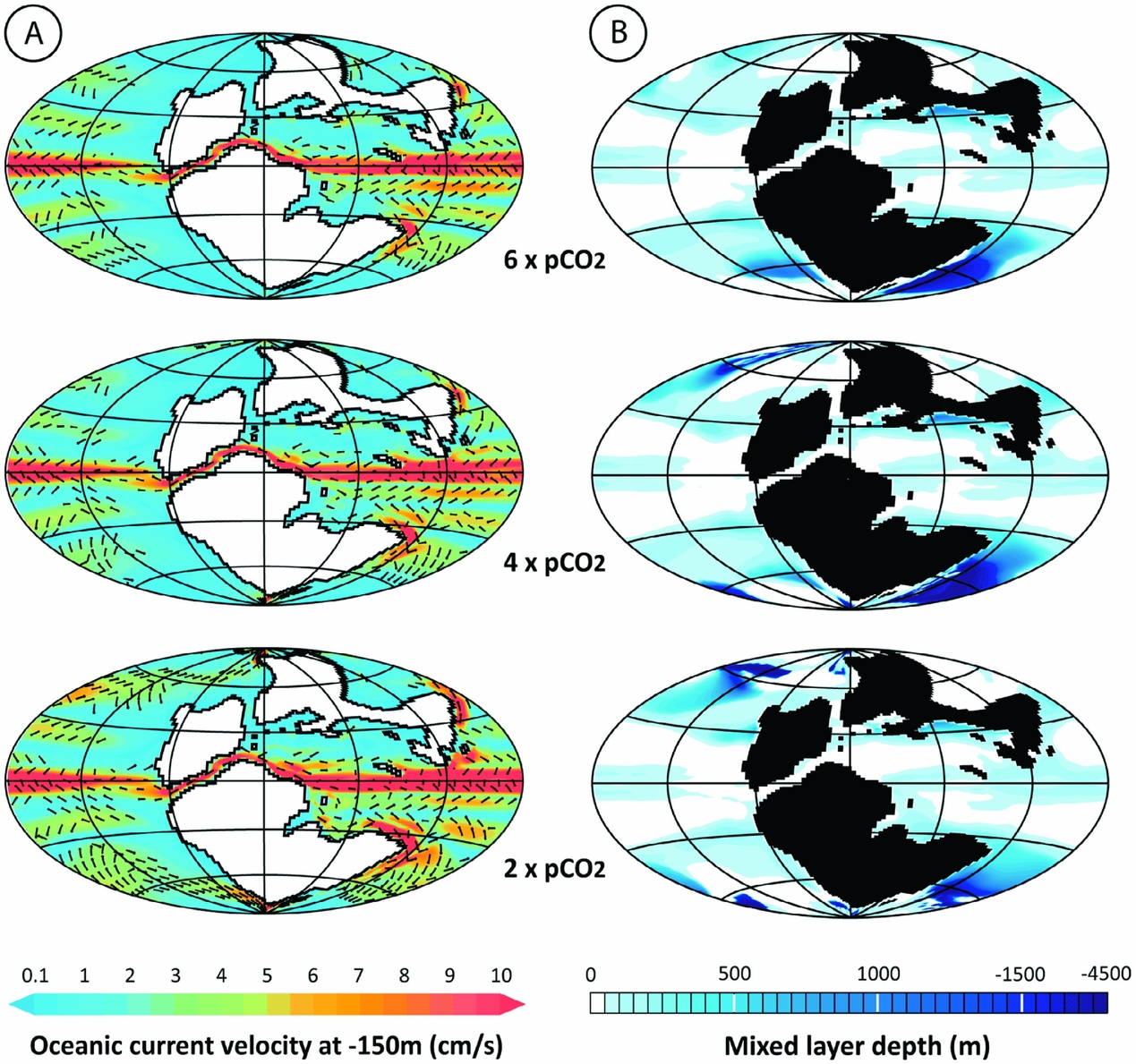
Velocity field in the first layer of the present-day ocean averaged over the last 100 years of simulation using three different bathymetries (submarine relief): (a) real bathymetry (variable depth) used as reference; (b) flat ocean floor fixed at −4000 m; (c) flat ocean floor fixed at −2000 m. After Perroud, Brunetti & Vérard (Reference Perroud, Brunetti and Vérard2015, fig. 5).

Similarly, the well-known models for biochemical cycles over the Phanerozoic (François & Walker, Reference François and Walker1992; and more recently the GeoCarbSulf model of Berner, Reference Berner2006) – including the cycles of carbon, sulphur, calcium, magnesium, phosphorus, oxygen and strontium – are based on the land and continental shelf distribution defined by Parrish (Reference Parrish1985), who combined the reconstruction maps of Scotese et al. (Reference Scotese, Bambach, Barton, Van der Voo and Ziegler1979) and Ziegler, Scotese & Barrett (Reference Ziegler, Scotese, Barrett, Brosche and Sündermann1983). Now, these models for biochemical cycles require quantifying the amount of accreted material at mid-oceanic ridges or the amount of subducted material at trenches. Again, those values cannot be properly estimated from a list of Euler parameters, and demand the use of a full plate tectonic model.
In this case as well, the best way to achieve the goal of modelling such cycles is first to couple an ad hoc full plate tectonic model with a global model of climate in order to quantify fluxes of various matter, and then to model biochemical cycles in relation to those fluxes.
6. Conclusions and perspectives
In science, it is difficult to say what is right, but one can say what is wrong. It is therefore essential to pinpoint any errors (i.e. mismatches between scenarios and data) of the different models and to propose alternative solutions. The validation or rejection of reconstructions can be done by compiling more geological data (sensu lato) but also by using other sources of data.
A great way to validate the choice made using plate tectonics is to generate lithofacies maps on top of the reconstructions. Despite the spatial resolution problem, the correlations necessary to create such maps (of the type of Ronov, Khain & Seslavinsky, Reference Ronov, Khain and Seslavinsky1984; Ronov, Khain & Balukhovsky, Reference Ronov, Khain and Balukhovsky1989; or recently Boucot et al. Reference Boucot, Xu, Scotese and Morley2013 in relation to the PaleoMap Project: http://www.scotese.com, for instance) are very effective in detecting areas that can cause problems. Such work is thus not only fantastic but fundamental. Unfortunately, such work – as crucial as it is – may border on circular reasoning, because lithofacies data can be used beforehand to constrain the reconstructions (semi-quantitative data). It is probably more appropriate to collect more data and check each time whether they are consistent with the data already used. The modeller(s) is(are) relatively limited in his/her(their) ability to compile large amounts of data. It would therefore certainly be wiser to open a platform (of the type of GEO – GEOSS, https://www.earthobservations.org, EarthCube, http://earthcube.org, or the IGCP 509 database system, http://sil.usask.ca/Databases.htm; Eglington, Reddy & Evans, Reference Eglington, Reddy, Evans, Reddy, Mazumder, Evans and Collins2009) so that the scientific community can put the newly acquired data in their configuration of the past (using different models) on one hand, and so that the data can feed the databases used by the modeller(s) on the other hand.
Now, the use of large data compilation is likely to be a dead end when associated with reconstructions using the ‘single control approach’. It is stressed that a model of reconstructions of the Earth through the geological past cannot be reduced to a list of Euler poles. Reconstructions must rest on the plate tectonic theory. The ‘dual control approach’ allows proposing reconstructions physically coherent with geodynamic scenarios imagined in 3D (on the global sphere, from the Earth's surface to the Earth's interior). It requires a global coverage that highly reduces the degree of freedom of the system, and involves the use of synthetic data (e.g. Vérard et al. Reference Vérard, Hochard, Baumgartner and Stampfli2015a).
Beyond this work, it seems clear that the next frontier is to couple the plate tectonic models to other models (see Vérard, in press), which in turn can shed light on the validity of the choices and the assumptions made to reconstruct the past. The coupling of plate tectonic models with other global models requires specific architecture. Not only will plate tectonic models have to take feedback from other models into account, but they must also be designed so that each feature must keep track of its past evolution, i.e. must remember its inheritance. The forthcoming Panalesis model resumes the know-how developed at the University of Lausanne, including the definition of tectonic plates all around the globe at all reconstructed ages, but, contrary to the UNIL model, it is designed to remember inheritance stemming from previous reconstructions and to be ready for further developments in association with other numerical models such as the following.
Mantle convection models require plate tectonic models as boundary layers on the surface. In return, convection models provide independent datasets that can confirm or reject some reconstructions, especially when comparing the results of convection models with seismic tomography. The EarthByte model is quite ahead on this topic (e.g. Bower, Gurnis & Seton, Reference Bower, Gurnis and Seton2013; Flament, Reference Flament2014; Bower, Gurnis & Flament, Reference Bower, Gurnis and Flament2015 for recent papers), but work has also been carried out, for instance, with the UNIL model (Hafkenscheid, Wortel & Spakman, Reference Hafkenscheid, Wortel and Spakman2006; P. Webb, unpub. Ph.D. thesis, Univ. Cardiff, 2012). The mantle convection models can provide, in addition, heat flow data (e.g. Davies & Davies, Reference Davies and Davies2010; Davies, Reference Davies2013) that have important implications for the evolution of basins (Müller, Reference Müller2010) or ocean chemistry (Müller et al. Reference Müller, Dutkiewicz, Seton and Gaina2013).
Palaeo-stress models run at the scale of tectonic plates can also serve as sources of data to support or refute the geodynamic scenarios. Here, too, work has already been done on the Australian plate with the EarthByte model (Müller, Dyksterhuis & Rey, Reference Müller, Dyksterhuis and Rey2012) and on the IndoEuropean plate with the UNIL model (Warners-Ruckstuhl, Govers & Wortel, Reference Warners-Ruckstuhl, Govers and Wortel2012; Warners-Ruckstuhl, Govers & Wortel, Reference Warners-Ruckstuhl, Govers and Wortel2013; Hafkenscheid et al. Reference Hafkenscheid, Warners-Ruckstuhl, van Oosterhoot, Bergman, Davies, Govers, Hochard, Kennan, Ross, Stampfli, Vérard, Webb and Wortel2013). In addition, numerical models may have to be used – i.e. if not coupled at least used in a more systematic way – to constrain the geometry of the plate boundary, in particular in terms of the definition of synthetic mid-oceanic ridges (as done, in particular, by Gerya, Reference Gerya2013).
The definition of palaeotopography (bathymetry and hypsometry) is also crucial not only for the palaeogeography itself but as input data in many other numerical models. Three approaches are possible: (1) a qualitative approach of drawing topographies ‘by hand’ as does Ronald Blakey (CPGeosystems model); (2) a more quantitative approach based, for example, on analyses of fission tracks, exhumation rates, etc. (e.g. Braun et al. Reference Braun, van der Beek, Valla, Robert, Herman, Glotzbach, Pedersen, Perry, Simon-Labric and Prigent2012, Reference Braun, Simon-Labric, Murray and Reiners2014 for the use of such data and the development of an erosion model). This method is probably more relevant to the local scale but difficult to apply on a global scale, because such data cannot be obtained anywhere on the globe for any geological time; (3) a ‘synthetic’ approach as proposed by Vérard et al. (Reference Vérard, Hochard, Baumgartner and Stampfli2015b). The idea is opposite to the previous one, and consists of assuming that, at the first order, the reliefs follow mathematical rules applicable all around the globe for all ages. By modulating these reliefs with the definition of palaeoclimate, it should be possible to compare the synthetic data to quantitative data (e.g. fission tracks) and to identify areas where other factors may come into play (e.g. dynamic topography).
Climate models are therefore needed to understand climate change on Earth over long periods of time, and needed to constrain other numerical models. Although palaeoclimate simulations have been performed for many years (e.g. Chandler, Rind & Ruedy, Reference Chandler, Rind and Ruedy1992; Ross, Scotese & Otto-Bliesner, Reference Ross, Scotese and Otto-Bliesner1992; Fluteau et al. Reference Fluteau, Besse, Broutin and Ramstein2001; Markwick & Valdes, Reference Markwick and Valdes2004; Donnadieu et al. Reference Donnadieu, Goddéris, Pierrehumbert, Dromart, Fluteau and Jacob2006b; Fluteau et al. Reference Fluteau, Ramstein, Besse, Guiraud and Masse2007; Markwick, Reference Markwick, Williams, Haywood, Gregory and Schmidt2007; Sellwood & Valdes, Reference Sellwood and Valdes2008; Le Hir et al. Reference Le Hir, Donnadieu, Goddéris, Meyer-Berthaud, Ramstein and Blakey2011; Goddéris et al. Reference Goddéris, Donnadieu, Lefebvre, Le Hir and Nardin2012; Pohl et al. Reference Pohl, Donnadieu, Le Hir, Buoncristiani and Vennin2014; Brunetti, Vérard & Baumgartner, Reference Brunetti, Vérard and Baumgartner2015), real tectonic–climate interaction has not yet been proposed, although work is currently in progress to implement this aspect in the forthcoming Panalesis model.
Tectonic–climate interaction, however, can only be considered through the creation of an erosion–sedimentation model. Ideally, the reconstruction of the past should define 3D models where the geology of each region is fully described (in x, y, z), and in particular, where geology at exposure is known. Clearly, this goal seems unattainable, at least in the short or medium term. However, pioneering works (e.g. Ronov et al. Reference Ronov, Khain, Blukhovsky and Seslavinsky1980; Flögel, Wold & Hay, Reference Flögel, Wold and Hay2000; Hay et al. Reference Hay, Wold, Söding, Flögel, Merriam and Davies2001) have suggested axes of research for this topic. Crudes approximations are currently being considered (Panalesis model), and hopefully will capture the first-order effects.
Furthermore, erosion–sedimentation and palaeoclimates are very dependent on the vegetation. The plate tectonic models will also require coupling with continental vegetation models such as BIOME4 (Kaplan et al. Reference Kaplan, Bigelow, Prentice, Harrison, Bartlein, Christensen, Cramer, Matveyeva, McGuire, Murray, Razzhivin, Smith, Walker, Anderson, Andreev, Brubaker, Edwards and Lozhkin2003) or marine models such as Darwin (Follows & Dutkiewicz, Reference Follows and Dutkiewicz2011; http://darwinproject.mit.edu). Similarly, the plate tectonic models may constrain evolutionary models of faunas (e.g. Kergoat et al. Reference Kergoat, Bouchard, Clamens, Abbate, Jourdan, Jabbour-Zahab, Genson, Soldati and Condamine2014), and conversely the passage of certain fauna from one region of the globe to another are useful to validate reconstructions.
Finally, other global models will have to be coupled or at least used as input data or output data for the purpose of validation. This applies, in particular, to geochemical models related to climate such as GeoCarb (Berner, Reference Berner1998, Reference Berner2006) or GeoClim (Donnadieu et al. Reference Donnadieu, Goddéris, Pierrehumbert, Dromart, Fluteau and Jacob2006a; Donnadieu, Goddéris & Bouttes, Reference Donnadieu, Goddéris and Bouttes2009), geochemical models related to magmatism, but also astronomical models like La2010 (Laskar et al. Reference Laskar, Fienga, Gastineau and Manche2011; and see also Shaviv & Veizer, Reference Shaviv and Veizer2003).
In short, the new generation of global plate tectonic models can only be achieved by combining many teams working on a variety of topics. The coming decade will surely see a quantum leap in this field of research.
Acknowledgements
I gratefully thank the editor, Guido Meinhold, for his time and energy. I also want to thank Christopher Scotese for his kindness and for helping improve the manuscript, in particular by providing me with useful information. It was very constructive. I acknowledge two additional anonymous reviewers for their useful comments.