





Introduction
Alpine glaciers store precipitation as ice and release it as meltwater to the downstream environment. A key component of this mechanism is the subglacial drainage network, which impacts glacier dynamics through its seasonal evolution (Anderson and others, Reference Anderson2004; Bartholomaus and others, Reference Bartholomaus, Anderson and Anderson2008), and even beyond the scope of one melt season (Maier and others, Reference Maier, Andersen, Mouginot, Gimbert and Gagliardini2023). However, measuring the morphodynamics of the subglacial drainage network at high spatial and temporal resolution remains a challenge (Rada and Schoof, Reference Rada and Schoof2018; Church and others, Reference Church, Bauder, Grab and Maurer2021; Andrews, Reference Andrews2025).
In early spring, as snow and ice melt starts at slow rates and glacial discharge is still low, a distributed subglacial drainage system develops underneath the ice (Kamb, Reference Kamb1987; Walder and Fowler, Reference Walder and Fowler1994). Through the melt season, as melt rates increase and temporal peaks of meltwater are delivered to the bed via englacial drainage (e.g. via moulins) (Harper and others, Reference Harper, Humphrey, Pfeffer, Fudge and O’Neel2005), differences in water pressure at the bed develop. High basal water pressure causes increases in glacier surface velocity through basal sliding (Iken and Truffer, Reference Iken and Truffer1997; Mair and others, Reference Mair, Nienow, Sharp, Wohlleben and Willis2002) as well as frictional melt (Röthlisberger, Reference Röthlisberger1972), where that water is in contact with ice. This allows more hydraulically efficient channels to develop (Fountain and Walder, Reference Fountain and Walder1998; Bartholomew and others, Reference Bartholomew, Nienow, Mair, Hubbard, King and Sole2010; Cuffey and Paterson, Reference Cuffey and Paterson2010) and therefore lowers flow velocities of the glacier again, once the water pressure is released through these newly developed channels (Anderson and others, Reference Anderson2004). Dye tracing suggests that this channelisation, as had been inferred from field data, extends progressively further upstream during the melt season (Nienow and others, Reference Nienow, Sharp and Willis1998). Empirical analyses (Rada and Schoof, Reference Rada and Schoof2018) confirm that such networks develop, and several studies show that their extent can be modelled (e.g., Walder and Fowler, Reference Walder and Fowler1994; Schoof and others, Reference Schoof, Hewitt and Werder2012; Werder and others, Reference Werder, Hewitt, Schoof and Flowers2013; Hoffman and others, Reference Hoffman2016). Current attempts to model this dynamic behaviour still demand a non-static inclusion of locations of subglacial cavities and channels, which are challenging to obtain and validate (Anderson and others, Reference Anderson2004; Roldán-Blasco and others, Reference Roldán-Blasco, Gimbert, Gagliardini and Gilbert2025).
Theoretical models of subglacial drainage can be validated through experiments identifying channel structure and obtaining a more detailed understanding of the evolution of the drainage system. Subglacial channels are, however, difficult or even impossible to access, and cost- and time-intensive to detect from above. Recent studies have used ground-penetrating radar on a large scale to capture bedrock elevation and glacier thickness (Grab, Reference Grab2020), which allows more effective theoretical modelling of channel location, as well as direct measurement of subglacial water flow on a small but detailed scale (e.g., Church and others, Reference Church, Bauder, Grab and Maurer2021; Egli and others, Reference Egli, Irving and Lane2021; Klahold and others, Reference Klahold, Racz, Ruols and Irving2026). These approaches can deliver rich at-a-point-in-time images of subglacial drainage networks. Nevertheless, radar waves can be back-scattered by metagranitoid rocks or water-filled voids, as well as absorbed by clay-rich debris (Woodward and Burke, Reference Woodward and Burke2007; Egli and others, Reference Egli, Irving and Lane2021), and therefore may not reach down to the glacier bed.
Seismic studies are low in impact and cost and can provide a temporally and spatially rich evaluation of seismic activity from multiple sources on a glacier. Continuous experiments have identified structures in ice (Nanni and others, Reference Nanni, Roux, Gimbert and Lecointre2022) and recorded dynamic events on alpine glaciers, such as basal ice quakes (Stuart and others, Reference Stuart, Murray, Brisbourne, Styles and Toon2005; Walter and others, Reference Walter, Deichmann and Funk2008) or stick-slip events (Weaver and Malone, Reference Weaver and Malone1979; Gräff and Walter, Reference Gräff and Walter2021). Recently, new fibre-optic and machine-learning-based techniques have been tested to estimate subglacial runoff directly from the glacier surface (Manos and others, Reference Manos2024). To monitor the subglacial drainage network, seismic methods have already been used with success to identify the origins of tremor (Lindner and others, Reference Lindner, Walter, Laske and Gimbert2020) and singular subglacial channels (Gimbert and others, Reference Gimbert2021; Nanni and others, Reference Nanni, Gimbert, Roux and Lecointre2021). Gimbert and others (Reference Gimbert2021) and Nanni and others (Reference Nanni, Gimbert, Roux and Lecointre2021; Reference Nanni, Roux, Gimbert and Lecointre2022) have applied a source localisation technique using a grid-shaped network of seismic sensors on a glacier surface to locate subglacial water flow and crevasse structures. The approach, called matched field processing (MFP), compares phase delays of recorded seismic waves to simulated phase delays from multiple starting points at the depth of the glacier bed. The probabilistic approximation of the true source location from these starting points enabled the identification of a main subglacial channel below Glacier d’Argentière (France), motivating further attempts to detect complex dendritic subglacial drainage structures.
The aim of this study is to investigate the subglacial drainage network of Glacier d’Otemma. The objective is threefold: (i) to test whether more complex, multiple subglacial channels can be identified following Nanni and others (Reference Nanni, Gimbert, Roux and Lecointre2021) using MFP on different formations of seismic sensors; (ii) to compare the results to those obtained by a classical beamforming analysis; and (iii) to trace the evolution of the subglacial drainage system of Glacier d’Otemma throughout the melt season. To do so, we collected seismic data from a network of supraglacial seismic sensors over a period of six weeks during July and August 2024, thereby imaging the subglacial drainage network progressively throughout an inferred transition from a distributed to a channelised structure.
Field experiment
Glacier d’Otemma, with a length of about six km, is one of the largest Swiss glaciers. It is situated in the Canton Valais between 2550 and 3000 m elevation. Ground-penetrating radar data from Grab (Reference Grab2020) suggest an ice thickness of up to 300 m in the upper part of the glacier, with an average yearly loss rate between -0.8 and -2 m of water equivalent (m w.e.) (Linsbauer and others, Reference Linsbauer2021; Cremona and others, Reference Cremona2025) in the last five years. Based on a borehole measurement (Fig. 1a), we identify an ice thickness of around 130 m in our area of interest, for which the GPR data suggest a similar range between 100 and 150 m (Grab, Reference Grab2020). The area is located approximately one kilometre upstream from the glacier terminus, where we installed the sensors (Fig. 1a).
To identify the location of the subglacial drainage network under the glacier with seismic data, we installed four configurations of 21–28 seismic receivers in boreholes of 30 cm depth on the glacier surface at an average altitude of 2600 m (Fig. 1a). We have used SmartSolo IGU-16HR 3C (three-component) 4.5 Hz seismic sensors (SmartSolo, 2025), hereafter referred to as ‘nodes’, with a sampling rate of 500 Hz. The entire duration of recording was 30 days over a period of six weeks, starting on 18th July 2024. Due to rapid melt and no snow cover on the glacier surface, the sensors had to be reinstalled every 72 hours. Not all recordings were used for the analysis; for configuration two, we were unable to set up all sensors over the full glacier width, so the coverage of the survey area was incomplete.
To obtain a wide, evenly spaced coverage of our survey area for the MFP approach, the first configuration comprised a 4  $\times$ 8 grid-shaped network of seismic nodes spanning the width of the glacier tongue, with 60 m spacing between the sensors (Fig. 1a). The sensor distance for both methods had been selected based on recent experiments which detected wave velocities in ice. A distance between 30 and 70 m allows the detection of minimum S-wave lengths as low as 35 m for a frequency range between 5 and 40 Hz (Fig. 1a), assuming P- and S-wave velocities in ice to be
 $3400-3900\;\mathrm{ms}^{-1}$ and
 $1400-1900\;\mathrm{ms}^{-1}$ according to Booth and others (Reference Booth2020); Walter and others (Reference Walter2020); Hudson and others (Reference Hudson2021); Xie and others (Reference Xie2024). The network was active for one week from 18th July to 24th July, providing reliable seismic data for the first 72 hours, during which the seismic node was not yet tilted by supraglacial melt.
The second main configuration of sensors aimed at obtaining high accuracy in determining the back azimuth of the origin of dominant seismic sources. It encompasses three triangular networks of seven seismic nodes, hereafter called ‘arrays’, each with distances of 30–100 m, covering the full width of the glacier in our area of interest and allowing triangulation of signal in between (see Fig. 1a). The configuration was active for nearly three weeks starting on 18th August, and sensor distances were modified twice (60 m, configuration 3; 30 m, configuration 4) to allow different wavelengths to be recorded.
To monitor subglacial meltwater and suspended sediment export from the glacier, we installed a Campbell Scientific gauging station with an OBS300 turbidity sensor and a CS451 pressure transducer recording at two minutes intervals 500 m downstream of the glacial terminus. Precipitation data from MeteoSwiss (2025) are available for the station ‘VSCHA’, six km away from the study site, and temperature data from a second station ‘GSB’, at a distance of 23 km.
Map of the seismic experiment on Glacier d’Otemma, Valais, Switzerland (CRS: WGS 84/UTM 32N): The upper left map shows the outline of Switzerland with the location of Glacier d’Otemma marked by a red dot. The lower left map zooms into the valley, showing the outline of Glacier d’Otemma (blue line) as well as our study area marked with a white box. We used two main configurations of nodes (Configurations one and four), as represented in the main map by the dark and light grey triangles, which we slightly modified at different stages. Figure 1b shows the duration of the different configurations over time. In configuration two, we could only install half of the sensors of configuration one after they had melted out, so we cannot use it for the MFP analysis. The blue square represents the location of our hydrological gauging station in front of the glacier terminus. The pink marker shows node 20821, which is used later as an example for seismic traces.

Figure 1 Long description
The map shows Glacier d’Otemma in Switzerland, marked with a blue outline. The first inset map highlights Switzerland with a red dot indicating the glacier′s location. The second inset map shows the full extend of the Glacier d’Otemma as well as the area of interest for our project. The main map displays various elements: seismic sensors marked by triangles, borehole locations by red circles and the gauging station by a blue square. The first, grid-shaped configuration of seismic sensors on the glacier surface is marked by grey triangles. The fourth configuration of three arrays of seismic sensors (Array 1, Array 2, Array 3) are labeled and marked by light grey triangles. The map uses UTM coordinates with axes labeled UTM North (m) and UTM East (m). The legend explains symbols: glacier outline (blue line), gauging station (blue square), borehole (red circle), first configuration of seismic sensors (grey triangles) and fourth configuration of seismic sensors (light grey triangles). Below the map, a timeline shows the duration of different configurations (Config. 1, Config. 2, Config. 3, Config. 4) over time, from 18th July to 23rd August, with specific dates marked for each configuration change.
Methods
To identify the structure and evolution of the subglacial drainage network, we apply and compare two cross-correlation approaches to locate seismic sources: beamforming and matched field processing (MFP). Beamforming is a seismological approach to separate noise from coherent signal (Rost and Thomas, Reference Rost and Thomas2002) with little a priori knowledge about the wave characteristics needed, based only on the plane-wave assumption and the homogeneity of the signal and medium (Métaxian and others, Reference Métaxian, Lesage and Valette2002). With this approach, we want to identify the origins of dominant seismic sources from the glacier surface and trace their variation in time. The second approach, MFP, is also suited to identify spherical wavefronts and can thus be applied in the near field. The true source location is iteratively approximated on a coordinate level and further reduces noise when appropriately parametrised (Baggeroer and others, Reference Baggeroer, Kuperman and Mikhalevsky1993). We aim to obtain two-dimensional maps of source densities for our area of interest with this technique.
For both beamforming and the MFP approach, we select the frequency range of 3–7 Hz, according to Nanni and others (Reference Nanni, Roux, Gimbert and Lecointre2022) and previous studies which identified (subglacial) river signals in similar frequency ranges (Bartholomaus and others, Reference Bartholomaus, Amundson, Walter, O’Neel, West and Larsen2015; Mancini and others, Reference Mancini2023). To ensure a good fit in this frequency band, we investigate the choice of both our seismic methods and compare results of different frequency bands. Even though the common frequency band for turbulent alpine streams had been tested in the pro-glacial as well as subglacial environment (Nanni and others, Reference Nanni2020; Mancini and others, Reference Mancini2023), we needed to get an overview of seismic activity in certain frequency ranges and their variations. Therefore, we investigated the accumulated amplitude of different frequency bands between 1 and 125 Hz to observe their correlation with the melt behaviour of the glacier.
Beamforming
To retrieve the apparent seismic velocity and back azimuth (azimuth towards the source) estimates with beamforming, we process data of each triangular array of seismic nodes (Configurations 3 and 4 in Fig. 1) on the glacier surface, following the approach of Métaxian and others (Reference Métaxian, Lesage and Valette2002). For a given time window, the time delay  $\tau_{ij}$ between signals recorded by two receivers
 $i$ and
 $j$ corresponds to the cross-spectrum phase
 $\varphi_{ij}(f)$ (e.g. Poupinet and others (Reference Poupinet, Ellsworth and Fréchet1984)):
 \begin{equation}\tau_{ij} = \frac{\varphi_{ij}(f)}{2\pi f}\end{equation}
where  $f$ is the frequency. We compute this time delay
 $\tau_{ij}$ for each station pair as a weighted linear fit of the cross-spectrum phase. The weight function
 $W$, defined by Frechet (Reference Frechet1985), weights the cross-spectrum modulus
 $\lvert S_{ij}(f)\lvert$ according to its coherence
 $C_{ij}(f)$:
 \begin{equation}
W_{ij}(f) = \frac{\lvert S_{ij}(f) \rvert C^2_{ij}(f)}{1-C^2_{ij}(f)}
\end{equation}
The resulting time delays  $\tau_{ij}$ are associated with the relative position vector
 $\mathbf{r}_{ij} = (r_{ij} \, \sin \, \phi_{ij}, r_{ij} \, \cos \, \phi_{ij})$, where
 $r_{ij}$ and
 $\phi_{ij}$ are the distance and azimuth. Considering N stations, we obtain
 $N(N-1)/2$ time delays which are related to the apparent slowness vector
 $ \mathbf{s}$ as follows:
 \begin{equation}
\tau_{ij} = \mathbf{s} \cdot \mathbf{r}_{ij}
\end{equation}
To determine the apparent slowness vector, we solve the linear system of equations  $ \mathbf{s}= (-s \, sin \, \theta, -s \, cos \,\theta)$ where
 $\theta$ is the back azimuth of the dominant source. This approach is repeated over moving time windows, for which we tested five different window lengths (Appendix A1). The resulting estimations of back azimuth and apparent velocity per optimal windows of 16 seconds allow us to continuously trace the location and variability of dominant noise sources in our glacial environment.
We need to take a look at the fact that the beamforming method is based on a plane-wave assumption, which, with regard to the frequency band of 3–7 Hz, previously described S-wave velocities in ice (Booth and others, Reference Booth2020; Walter and others, Reference Walter2020; Hudson and others, Reference Hudson2021; Xie and others, Reference Xie2024) and a source at about 130 m depth, does not apply. Almendros and others (Reference Almendros, Ibáñez, Alguacil and Del Pezzo1999) did account for spherical wavefronts in beamforming, comparing the performance of plane wave and spherical wave solutions for sources in the near field, defined as less than three times the array aperture. Investigations of Almendros and others (Reference Almendros, Ibáñez, Alguacil and Del Pezzo1999) show that these variations in back azimuths between assuming a planar or a spherical wavefront range within a few degrees. As we are interested in general tendencies and diurnal variations of back azimuth and velocity estimations, these minor deviations do not impact the conclusions drawn from it. Further, Almendros and others (Reference Almendros, Ibáñez, Alguacil and Del Pezzo1999) define the critical distance of a source according to array aperture. Therefore, we tested the calculations of back azimuth and velocity on less sensors forming a smaller array with an aperture of 33 m, which is supposed to be sufficiently small to well resolve sources at about the glacier depth. To ensure that the estimated source back azimuths for subglacial turbulent streams can be considered legitimate, we did additional tests on higher frequency bands. Between 20 and 40 Hz, the sources are attributed to bedload transport (Tsai and others, Reference Tsai, Minchew, Lamb and Ampuero2012; Gimbert and others, Reference Gimbert, Tsai and Lamb2014; Dietze and others, Reference Dietze, Lagarde, Halfi, Laronne and Turowski2019; Nanni and others, Reference Nanni, Gimbert, Roux and Lecointre2021), which happens only in the subglacial channels, being uncorrelated with englacial or supraglacial melt processes. By adding these supporting experiments, we ensure the validity of the method for our purpose to see origins of the turbulent stream signal from the glacier surface.
Matched field processing
In order to localise the source, we then apply MFP on the same data. It approaches the potential source location according to the highest phase coherence between observed and modelled phase delays for a dense network of seismic stations (e.g., Vandemeulebrouck and others, Reference Vandemeulebrouck2010; Cros and others, Reference Cros, Roux, Vandemeulebrouck and Kedar2011; Jensen and others, Reference Jensen, Kuperman, Porter and Schmidt2011; Corciulo and others, Reference Corciulo, Roux, Campillo, Dubucq and Kuperman2012; Gradon and others, Reference Gradon, Moreau, Roux and Ben-Zion2019). We follow the approach defined in Gimbert and others (Reference Gimbert2021) and Nanni and others (Reference Nanni, Gimbert, Roux and Lecointre2021), which was designed for a similar purpose.
To identify the source origin for a given time window, we first compute the discrete Fourier transform of the data from each station and combine them in the vector  $\mathbf{d}(\omega)$, where
 $\omega$ is the angular frequency. We determined the cross-spectral density matrix
 $K$ as:
 \begin{equation}
K(\omega) = \mathbf{d}(\omega) \mathbf{d}^H(\omega)
\end{equation}
with  $H$ representing the conjugate transpose. When modelling the synthetic data, we assume a point source
 $a$ at the spatial location (
 $x, y, z$) and wave propagation from the source to the stations at the constant velocity
 $c$. In order to avoid local minima in the exploration of the model space, we perform the inversion using 36 starting points (
 $x_o,y_o,z_o,c_o$). For a given station, at a distance
 $r$ from the source
 $a$, the Greens function replica vector is:
 \begin{equation}
d(\omega, a) = \exp(\frac{i \omega r_{a}}{c})
\end{equation}
where  $c$ represents the medium velocity. Based on the replica vector
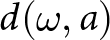 $d(\omega, a)$ and the cross-spectral density matrix
 $K(\omega)$, we measure the difference between the synthetic and observed phase delays with the Bartlett processor:
 \begin{equation}
B_{Bartlett}(\omega, a) =\sum_{\omega} | \mathbf{d}(\omega, a)^H K(\omega) \mathbf{d}(\omega, a)|
\end{equation}
The higher the Bartlett value is (ranging from 0 to 1), the higher is the cross-correlation between modelled and observed phase. It is the main quality indicator for each estimation of source location. We evaluate our estimations according to the Bartlett value and optimise source location and propagation velocity with a gradient-based minimisation algorithm (downhill simplex search, (Lagarias and others, Reference Lagarias, Reeds, Wright and Wright1998)). We apply this method to windows of one second with 50% overlap and process data packets of 24 hours to obtain stable estimates of permanent source locations throughout a day.
To better understand whether it is possible to compare the results of the different sensor positions (see Fig. 1a), we did synthetic tests for both main configurations, the grid-shaped network and the triangular arrays. We simulated a 5 Hz Ricker wavelet, emitted repeatedly at randomly varying time intervals around half a second. The seismic velocity in the ice was set to  ${\sim 1800 \ m s^{-1}}$, and we created three artificial source locations at the depth of the glacier bed. We added random noise to the synthetic trace with the same maximum amplitude as the one of the synthetic wave. For comparison, we ran the matched field processing for (1) pure random noise, (2) for only the synthetic sources emitting signal and (3) for the same signal within random noise. In a second test, we compared the random noise source detection for different frequency bands to ensure to see the same effect as Nanni and others (Reference Nanni, Roux, Gimbert and Lecointre2022), where with higher frequencies, they observed random seismic noise likely to be allocated closer to the starting points. With the help of these tests, we can better assess how much of the source pattern is due to changes in array geometry and what part of it could be due to changes in the subglacial hydrological network.
Hydraulic potential
To obtain a first-order approximation of plausible subglacial flow pathways against which to qualitatively compare the seismic results, we calculate hydraulic potential at the glacier bed following Shreve (Reference Shreve1972), using the approach in Egli and others (Reference Egli, Irving and Lane2021). The hydraulic potential is
 \begin{equation}
\Phi = \rho_w g (H - z) + c\, \rho_i g\, z
\end{equation}
where  $\rho_w$ and
 $\rho_i$ are the densities of water and ice,
 $g$ is gravitational acceleration,
 $H$ is the glacier surface elevation,
 $z$ the local ice thickness, and
 $c$ a pressurisation constant expressing the ratio of subglacial water pressure to the ice overburden pressure. In this formulation,
 $c$ is spatially uniform and therefore cannot represent spatiotemporal variations in pressurisation, but it provides a simple way to explore how potential gradients respond to the relative influence of surface slope, ice thickness gradients and the assumed subglacial water pressure. Because the true pressure distribution at the bed is unknown, we treat
 $c$ as a limited sensitivity parameter and compute potential fields for different ranges (
 $0.1 = \lt c = \lt 1.0$). For each field, we then derive a flow-accumulation map using a D8 flow routing algorithm. The resulting flow accumulation maps do not represent a hydrological model of the drainage network, but provide a first-order approximation of where subglacial water would be expected to concentrate under each assumed pressure ratio. We use them only for qualitative comparison with the horizontal patterns of seismic source locations. Ice thickness data are taken from the GPR-based dataset in Grab (Reference Grab2020), and glacier surface elevations from the 2024 Swisstopo Alti3D dataset (Swisstopo, 2024).
Hydrological and seismic recording of Otemma glacier, 17th to 19th August 2024: (a) The respective power spectral density plot of station 20821 as well as (b) the water level and (c) turbidity at the glacier outlet and (d) temperature and precipitation data from weather stations at a few kilometres’ distance. Station 20821 is located in array two on the northern side of the study area (see purple marker in Figure 1a).

Figure 2 Long description
Station 20821: The image a is showing a spectrogram with the vertical axis labeled Frequency [Hz]. The frequency axis shows tick labels at logarithmic scale from 1 to 100. The horizontal axis shows date and time tick labels from 17th August to 19th August at 6 hour intervals. A horizontal color bar above the plot shows seismic power in decibel from -180 to -150. The spectrogram contains periods of higher and lower seismic power, depending on time and frequency. Subfigure b shows the time series of water level [m]. The water level axis ranges from 0.0 to 0.3. The horizontal axis shows the same date and time tick labels as image a, from 17th August to 19th August at six hour intervals. The plotted line varies between about 0.1 and about 0.3, with a local high near 18th August at midnight and another rise approaching 19th August, midnight. The image C shows a the time series of turbidity [NTU]. The turbidity axis ranges from 0 to 1500 NTU. The plotted line stays near a low baseline for much of the period, with a sharp peak reaching close to 1500 near 18th August, midnight, then returning to lower values. The image D shows two overlaid series with a left vertical axis labeled Precip. [mm] and a right vertical axis labeled Temp. [C]. The precipitation axis ranges from 0 to 5mm. The temperature axis ranges from 0 to 20 degrees. The precipitation series appears as vertical bars, with a rain event detcted around 18th August, midnight.
Results
Here, we present the results by their progressive level of abstraction from the raw seismic data: (i) a spectrogram of the seismic activity recorded by an exemplary seismic node on the glacier surface; (ii) time series of dominant back azimuths and apparent wave velocities retrieved from the beamforming analysis; and (iii) MFP-based horizontal source location maps.
The seismic recordings on the glacier of several days over the course of six weeks show multiple short, impulsive rises in amplitude as well as more continuous, cyclic noise occurrences. Illustrated in three example days of recording, we observe how the seismic recordings react to lower and higher temperatures and, respectively, lower or higher discharge, as well as rainfall (Fig. 2). Starting from about 8:00 UTC, the water level in the proglacial stream is rising and corresponds well to a rising amplitude in a frequency band around 5 Hz, as well as 10–40 Hz. When the proglacial stream reaches its highest level on the 19th August, a second, intense noise pattern appears in a frequency range between 10 and above 100 Hz, lasting from 14:00 to about 16:00 UTC. The observed pattern is similar across stations.
Appendix B1 shows even more clearly that the frequencies below 10 Hz are almost continuously amplified, with a minor rise throughout midday. Contrary to that, the frequencies above 100 Hz vary the most in amplification, which closely follows the melt behaviour of the glacier. Similar patterns are observed for the seismic station on the ground (Appendix B2), close to the glacial terminus.
We follow these diurnal, cyclic occurrences of seismic noise further and investigate where they might originate. The beamforming analysis provides time series of dominant back azimuth (source azimuth) and apparent velocity values of our seismic data (Fig. 3). We observe that strong variations in dominant back azimuths occur during the early morning (03:00–09:00), along with apparent velocities up to  ${\sim 10.000 \ m s^{-1}}$, whilst air temperature and glacial discharge are low. The back azimuths later converge towards a stable orientation during the day (09:00–00:00). During those warmer hours, apparent velocities decrease to the range of
 ${\sim 1600 \ m s^{-1}}$ to
 ${\sim 7500 \ m s^{-1}}$, along with rising temperatures and discharge. The main velocity peaks are found around
 ${\sim 2250 \ m s^{-1}}$ and
 ${\sim \ 5050 \ m s^{-1}}$. The observed changes in both values, back azimuth and apparent velocity, closely follow variations of meteorological and hydrological parameters (glacial runoff, temperature and turbulence) throughout the day.
Beamforming inversion: Back azimuth (BAZ) and apparent velocity (a1–a3) of each array of seismic sensors (see Figure 1a) from 3 to 7 Hz with the corresponding probability density (PDF) (b1–b3) for a 24 hour window. In addition (c), we show the seismic trace of station 20821 in array two (purple marker in Figure 1a), filtered in the same frequency range and (d) the water stage, turbidity, precipitation and temperature records. Each time series of back azimuths and velocities shows clear diurnal changes with rather stable values throughout the high discharge period and shifts towards various back azimuths and velocities during the colder morning hours (05:00–07:00). The seismogram shows low noise, but several strong, punctual amplitude peaks during that time.

Figure 3 Long description
The image consists of multiple plots showing seismic and environmental data over a 24-hour period. The top section includes three scatter plots labeled a1, a2 and a3, representing back azimuth (BAZ) on the y-axis with units in degrees, ranging from 0 to 360. Colored points indicate detections, with color representing apparent velocity in kilometers per second, ranging from 1 to 10. To the right, plots b1, b2 and b3 display probability density functions (PDF) of back azimuth estimations for each array. Below these, plot c shows a seismic trace from Station 20821, filtered between 3 to 7 Hz, with normalised amplitude on the y-axis. The bottom plot, labeled d, presents time series data for water stage, turbidity, precipitation and temperature. The left y-axis is labeled Water stage [m], while the right y-axis includes Turbidity [NTU], Precipitation [mm] and Temperature [°C ]. Four lines represent these variables, showing diurnal changes and correlations. Key observations include shifts in BAZ and apparent velocity during colder morning hours and stable values during high discharge periods. The seismic trace shows low noise during colder morning hours with punctual amplitude peaks and higher amplitude of the seismic trace during high discharge periods , as well as environmental variables showing those diurnal patterns.
To identify possible source origins more reliably, we plot the number of dominant waves arriving from different orientations onto our three seismic arrays in Fig. 4a and compare them to the basal hydraulic potential calculations. In the early morning between 03:00 and 09:00 UTC, the back azimuths facing the glacier margins and hill slopes of the valley (NW and SE of the glacier) are dominating. Additionally, a large number of signals are arriving from a narrow 40–45 degree band for arrays two and three (mode of the distribution, symbolised by the black dot), matching the path of the subglacial stream that is predicted by the hydraulic potential. In the afternoon, between 14:00 and 16:00 UTC, the dominant noise sources concentrate towards the centre of the glacier (Fig. 4b) and almost no dominant sources from the side of the glacier are detected. Taking the velocity values into account, Fig. 4b suggests sources from shallow to 45 degree incidence angles during the day, whilst Fig. 4a suggests unidentified seismic sources approaching the surface at a steeper incidence angle than during the day.
Beamforming results projected onto the glacier surface: Distribution of back azimuths from the centre point of each seismic array from 05:00 to 07:00 (4a) and from 14:00 to 16:00 (4b) on 23rd August. The black dot shows the mode of the distribution, and the letters A1–A3 show the number of the array. The blue lines show the estimated hydraulic potential according to Shreve (Reference Shreve1972) using a pressurisation constant of one. We see a clear difference in dominant back azimuths in the early morning hours, which face glacier margins and the valley side slopes, compared to the afternoon hours, where all identified sources gather in the middle of the glacier.

Figure 4 Long description
Two maps display beamforming results on a glacier for 23rd August. The first map shows data from 05:00 to 07:00 and the second from 14:00 to 16:00. The legend indicates the times of the beamforming result with colors: 14:00-16:00 and 05:00-07:00. Seismic nodes are marked with triangles, representing the configuration from 22-25 August. Arrays A1, A2 and A3 are labeled. Hydraulic potential is shown as blue traces on the ice and glacier outlines are marked by a blue line. The mode of the beamforming estimations is indicated by black dots per array. The maps illustrate changes in back azimuth distribution between night and day, revealing different patterns of bback azimuth estimations for periods of lower and higher glacial discharge.
The back azimuth and velocity data show different distributions during the day and during the night. During the day, seismic sources at the centre of the glacier seem to dominate the surroundings. Other processes in the area become visible during the night, when the glacier is less active.
Our tests regarding the near-field condition for the seismic beamforming show only minor deviations for arrays of smaller aperture and different frequency ranges from these beforehand described findings. For a smaller array aperture (Appendix C1), the source back azimuths identified are almost the same as those found with the bigger array of sensors. The analysis of the 20–40 Hz frequency band with the beamforming approach shows the same back azimuth ranges, slightly less scattered (Appendix D1). Those insights help to further interpret our findings in the discussion section.
In order to determine the position of the observed glacial processes more exactly, we strictly define our area of interest to the glacier only and locate possible noise sources with MFP for windows of 24 hours. We first show the outcome of one day and its statistics, before we compare the results of nine days to see the evolution of the noise distribution. Figure 5 provides details of the MFP analysis for our reference day, 23rd August. The distribution of Bartlett values (MFP output) shows that the dominant number of sources have a low value of phase coherence between 0.01 and 0.3. We estimated a wide range of phase velocities, peaking around  ${1800 \ ms^{-1}}$ for all sources and at
 ${2000 \ ms^{-1}}$ for estimations with high accuracy. From a horizontal perspective, we can identify three locations where sources of phase coherence below 0.7 gather (marker A, B and C in Fig. 5b), most pronounced for location C. The three spots are elongated in the direction of glacier flow. Seismic events located with high precision (Bartlett value above 0.7) are found mostly along the supraglacial moraine, which extends parallel to the glacier flow (marker D in Fig. 5b). These events separate from the diffuse source pattern.
Matched field processing results for 23rd August 2024: Figure 5a shows statistics of the Bartlett values (MFP output; coherence between modelled and observed phase arrivals) and estimated phase velocities. Figure 5b provides a planimetric density map showing the density of estimated source locations. Three main noise features identified are marked by boxes with the letters A, B and C. The white points show the starting points for the gradient optimisation algorithm. The red dots show single sources detected with high accuracy, mostly close to the moraine, which spans the area within box D. The dotted grey line on Figure 5b shows the location of the profile through the glacier shown in Appendix E1.

Figure 5 Long description
Subfigure a shows two histograms. The left histogram shows the distribution of MFP output values, ranging between 0 and 1. The distribution of values peaks near 0.1 MFP output value at more than 10,000 observations and decays with rising MFP output values to less than 10 observations near 0.9 MFP output value. Red bars highlight MFP output values above 0.7. The right histogram shows the distribution of phase velocity values ranging between 0 and 4000 m/s. The number of observed phase velocity values peaks at around 1600 m/s, whilst the most observations of high accuracy have phase velocity values around 2000 m/s as indicated by the red bars. A legend below the histograms explains the use of color in the histograms: All (purple) and High Accuracy (red). Subfigure b shows a map with a density overlay and point markers. A color scale at right is shows source density, with values between 0 and 0.00002 . The map contains many small red dots mostly spread across the right half and central area of the map. White circles mark the starting points for the MFP algorithm across the map. Multiple triangle markers show the positions of the seismic sensors on the glacier. Four boxed regions are labeled A, B, C and D, showing features discussed in the caption. A legend in the upper right explains markers for: high accuracy, stations, starting points and profile cut.
We want to observe the possible change in this pattern of noise sources from 3 to 7 Hz, associated with turbulent water, throughout our survey period and compare it to the calculations of the hydraulic potential. The hydraulic potential model is slightly varied for the first three days in July, as we assume a transition from intermediate to strong subglacial water pressure according to glacial runoff records (Appendix F1). When investigating nine days of seismic data within a period of four weeks (Fig. 6), a short-term temporal stability of the noise distribution (1–2 days) and a long-term variation of source locations (over the course of weeks) becomes apparent. In mid-July, the distribution of noise sources is relatively equal over the area of interest, with one more pronounced noise spot at the southern glacial margin. In mid-August, the identified dominant sources are drawn towards this southern source spot. The low-density noise pattern over the full survey area is in retreat, leaving the northern part of the area with little source occurrence. Towards the end of August, the sources form a more distinct pattern, concentrating in three dominant zones by the end of the month. These three noise hot spots overlap with the modelled water paths calculated by the hydraulic potential (Shreve, Reference Shreve1972).
MFP density maps: Density of dominant noise sources for time windows of 24 hours from 18th July to 24th August 2024. In plots (6b to 6d), the seismic nodes form a grid-shaped network on the glacier surface. For (6e)–(6j), the sensors are arranged in triangular arrays. The base map shows basal flow accumulation maps derived from the hydraulic potential field computed with a pressurisation coefficient between 0.7 (6b–6d) and 1 (6e–6j), assuming an increased ratio of subglacial water pressure towards the end of August.

Figure 6 Long description
Nine maps display source density and hydraulic potential on a glacier from 18th July to 24th August, 2024. Source density is shown as a color gradient from 0 to 0.00002 and hydraulic potential is shown as a blue gradient. Grey triangles represent seismic nodes on the glacier: grey triangles for 18-20 July, dark grey triangles for 16-18 August and light grey triangles for 22-25 August. Maps b to d show nodes in a grid pattern, while maps e to j show nodes in triangular arrays. Higher source densities cluster towards the southern margin. Towards the end of August, three main source clusters across the glacier develop. Hydraulic potential lines show an alternative, independent approach to estimate to subglacial channel location.
Our synthetic test in Appendix G1 compares random noise and synthetic signal from three possible sources at the glacier bed to ensure our previously described results have validity across changing sensor configurations. The tests show that for random noise only, the grid-shaped network and the triangular arrays capture the highest signal coherence towards the centre of the seismic network. In both cases, the computation is most likely to converge and find a very low coherent result ( $ \lt 0.1$) for the minimum distance between all sensors, that is, the centre of the study area. When adding three synthetic sources, both configurations detect the sources at their correct positions with the same density patterns. The densities are slightly bigger for the triangular array set-up and blur a bit more into each other. Lastly, we tested random noise and signal together. Here, for both sensor configurations, the sources are detected in the correct location, even though random noise and signal have the same amplitude. The pattern found for the test with random noise is less precise than the one found for signal-only simulations, but the locations of the synthetic sources are nevertheless found. Equally as for signal-only, the triangular arrays have a slightly lower source precision. The second test on different frequency ranges in Appendix G2 shows, for lower frequency bands, as in our case 3–7 Hz, random noise is located widespread around the area of interest, with the highest density at the centre of the network. The higher the frequency, random noise tends to be located closer and closer to the initial starting point. These results give insight into the relation between sources, sensors and starting points, to be further discussed in the next section.
Discussion
Data that contain continuous and spatially rich information about subglacial channel formation and closure are still sparse, even though these processes affect glacial velocity and subglacial sediment transport. Our networks of seismic sensors draw a detailed picture of ground motion and allow interpretation of the behaviour of water flow below the glacier.
Raw seismic data corresponding to glacier runoff cycles
The spectrogram of the seismic nodes on the glacier surface (Fig. 2) shows a simultaneous rise of noise in frequency bands between 3 and 40 Hz with the diurnal cycle of glacier runoff. We relate the continuous signal in the frequency bands below 10 Hz to turbulent stream noise and above 10 Hz to bedload transport, according to previous studies (Tsai and others, Reference Tsai, Minchew, Lamb and Ampuero2012; Gimbert and others, Reference Gimbert, Tsai and Lamb2014; Dietze and others, Reference Dietze, Lagarde, Halfi, Laronne and Turowski2019; Nanni and others, Reference Nanni, Gimbert, Roux and Lecointre2021). Signal from supraglacial runoff is likely found at higher frequency bands above 50 Hz, as described by Podolskiy and others (Reference Podolskiy, Imazu and Sugiyama2023). According to those frequency ranges from previous research, we explain the highly amplified activity window of two hours between 14:00 and 16:00 in the frequency band 20–50 Hz to intensive bedload transport activity (Burtin and others, Reference Burtin2011; Roth and others, Reference Roth, Brodsky, Finnegan, Rickenmann, Turowski and Badoux2016), and we identify an intense activity of supraglacial melt at this time window as well for frequency bands above 50 Hz. According to these findings, the seismic noise detected from sensors on the glacier surface is directly associated with the glacial melt cycle, whilst different contributions to the melt output can be differentiated by frequency band. They can therefore provide a basis for identifying subglacial stream noise with our two seismic approaches, similar to those in Lindner and others (Reference Lindner, Walter, Laske and Gimbert2020); Nanni and others (Reference Nanni2020); Reference Nanni, Roux, Gimbert and Lecointre2022).
Source back azimuths driven by glacial melt cycle
The estimations of back azimuth and apparent velocity from the beamforming analysis show a clear diurnal variation, coherent with the on- and offset of glacial melt, suggesting that it is detecting the hydrological processes. The observed velocity variations of the beamforming analysis indicate that waves arrive at a shallower incidence angle during the daytime, between 30-90 degree for P waves ( ${\sim 3800 \ m s^{-1}}$) and 13–90 degree for S-waves (
 ${\sim 1800 \ m s^{-1}}$), when surface melt and discharge rates are high. During the night, they arrive at steeper angles down to 22 degrees for P- and 10 degrees for S-waves. We also observe velocities below the assumed
 ${\sim 1800 \ m s^{-1}}$ for S-waves, which can be attributed to surface waves in ice ranging around
 ${\sim 1600 \ m s^{-1}}$ (Sergeant and others, Reference Sergeant2020). Our results suggest that the supraglacial melt activity contributes to increasing subglacial stream noise by adding water through moulins and englacial channels to the subglacial drainage system during the warm hours of the day. This observation changes between day and night. During the night, the scattered back azimuths between 3 and 7 Hz suggest that the turbulent stream noise is no longer being the dominant seismic source. The highest number of observations during the night is found in various directions, whilst high apparent velocities indicate the arrival of waves at a smaller incident angle. For arrays two and three, the highest number of sources is found in a narrow back-azimuth band of about 45 degrees, pointing in the direction of the estimated subglacial stream position (black line indicating mode of distribution in Fig. 4). We interpret this as a possible local signal from the subglacial stream at nighttime for each array for the closest subglacial channel, within a greater variety of other dominant, unidentified sources, all reaching the sensors at a steep incidence angle. Back azimuths are less scattered during the day, suggesting that turbulent stream noise dominates the entire noise environment. These observations confirm that during the majority of the day, turbulent stream noise dominates the seismic signal in the frequency band from 3 to 7 Hz. Its continuity and correlation with meteorological parameters allow us to further use this frequency band for more detailed analysis of the location of the turbulent stream signal.
The complementary test for the beamforming analysis on higher frequency bands and for smaller array apertures confirms that the potential biasing of the results by the near-field condition does not influence our findings. The differences in results between an array of bigger and smaller aperture are marginal (Appendix C1). The sources in a 20–40 Hz frequency band, associated with bedload transport, are found in the same back azimuth ranges with less variation from the dominant direction (Appendix D1). One possible cause of the higher scatter in the frequency band 3–7 Hz could be the additional contribution of turbulent stream noise from the englacial channels. By observing the similar backzimuth estimations for both frequency bands, we can make sure we are observing the same source location in the near and in the far field, and that englacial channels don’t majorly disturb our source location for subglacial channels. This provides us with confidence that the results are valid, nevertheless the possibility to observe sources in the near-field.
Two-dimensional evolution of the subglacial drainage network
The MFP output produces maps of dominant source locations for the frequency range 3–7 Hz, associated with turbulent streams, over four weeks from a horizontal perspective. The distribution of noise sources from the glacier surface evolves from being more widely distributed to forming three distinct noise spots. One possible explanation could be the evolution of the subglacial drainage system. The gauging station at the glacial terminus records a slow rise in daily peak discharge from the end of July towards mid-August, followed by a sudden stronger increase in daily water level change observed towards the 28th August (Appendix F1). This rise in glacial discharge and suspended sediment aligns well with former observations of increased glacial meltwater export once an efficient drainage system develops (Fountain and Walder, Reference Fountain and Walder1998; Bartholomew and others, Reference Bartholomew, Nienow, Mair, Hubbard, King and Sole2010; Cuffey and Paterson, Reference Cuffey and Paterson2010). The three dominant noise spots found towards 22nd August align with the estimations of local hydraulic potential (Shreve, Reference Shreve1972), representing high basal water pressures, which had proven applicable for Glacier d’Otemma (Egli and others, Reference Egli, Irving and Lane2021; Jenkin and others, Reference Jenkin2023).
Whilst the horizontal source distribution suggests a more simple visual interpretation, the vertical perspective is less clear. As we had no sensors at depth of the glacier, we can resolve this perspective less good. The highest source density can be found on the surface or close to the surface of the glacier, around an altitude of 2680 m (Appendix E1). We explain this observation by the wave characteristics for seismic sources at the glacier bed: the number of identified sources peaks at velocities of  ${\sim 1800 \ m s^{-1}}$. This observation is coherent with the dominant wave velocities described for S-waves in ice (Booth and others, Reference Booth2020; Walter and others, Reference Walter2020; Hudson and others, Reference Hudson2021; Xie and others, Reference Xie2024). To characterise the wave types which they identified, Nanni (Reference Nanni2020) investigated the geometric attenuation of events identified in their MFP experiment. They found that below 10 Hz, attenuation values are high, around one, which is typical for body waves (Stein and Wysession, Reference Stein and Wysession2003). These findings support the assumption that we are mainly recording S-waves on the glacier surface. Locating these sources vertically is potentially hindered by the wavelength when assuming S-waves at a speed of
 ${\sim 1800 \ m s^{-1}}$ (initial input velocity) in the frequency range between 3 and 7 Hz with wavelengths of around 250–500 m. At this length, which is approximately twice the glacier thickness, the signal of bed sources might not be vertically distinct from a source at the surface, and therefore, the depth of the source cannot be reliably resolved (Appendix E1). Similar to the beamforming approach, a reliable vertical localisation of sources at the glacier bed could be achieved by installing deep sensors in the ice.
When validating the source estimations of the MFP analysis, the cross-correlation between modelled and observed wave phases (Bartlett value) acts as points of reference. As the subglacial stream represents one or several elongated, noisy sources, our main focus will be results at Bartlett values below 0.5, which represent noisier wave arrivals instead of punctual, clearly identifiable events. Whilst we mostly observe values in the lower coherency range, MFP also provides a lower number of values with high accuracy (red dots in Fig. 5b), which are located almost entirely around the area of supraglacial moraine. Nanni and others (Reference Nanni, Roux, Gimbert and Lecointre2022) investigated the horizontal accuracy of the source locations (identified with MFP in a comparable seismic network) with respect to wavelength  $\lambda$ and found a higher accuracy than expected: for crevasse events of up to
 ${\lambda/18}$ and other events around
 $\lambda/7$. The investigation of the exact timing of these events could give more insight into possible mechanisms at play, e.g. rock movement due to supraglacial melt or crevassing.
Effects of array geometry and starting points on the MFP analysis
Throughout our field experiment, we had set up four different geometric configurations of seismic nodes on the glacier surface, of which three were used for this analysis. One central question regarding the results is whether and how much the change in sensor geometry affects the results of the MFP analysis.
Our tests with synthetic data (Appendix G1) show that punctual, clearly distinct sources can be identified in equal positions with both main sensor configurations, grid-shaped networks and triangular arrays of sensors. More than that, noise at equal intensity will be filtered out and does not much affect the efficiency of MFP to detect the sources. We see a small difference between the performance of the grid-shaped network and the triangular arrays for both sources only and sources with random noise. The source positions are slightly less accurate for the arrays, estimating source density with more scatter around the true source location. When looking at noise only, the triangular arrays identify the noise cloud more towards the centre of the area of interest, whilst for the grid-shaped network, the noise is found more widespread. These tests are convincing us that the array configuration has only a minor effect on the results. During the interpretation of the results, we should remind ourselves that those tests are not representing the real noise environment, as our real sources are less distinct from noise. Nevertheless, for the scale at which we interpret the results in this study, neither the small inaccuracies in source detection nor the difference in noise pattern between array setups seem to impact the findings too much. On the contrary, the sources found with triangular arrays separate more clearly, which suggests that the distinctness of the real sources could have increased.
The comparison of the MFP in estimating the origin of synthetic random noise at different frequency bands (Appendix G2) shows an equal effect as described by Nanni and others (Reference Nanni, Roux, Gimbert and Lecointre2022). The higher the frequency, the more likely the MFP converges towards a source position close to the starting point. At lower bands, including our choice of 3–7 Hz, the random noise is located less punctual, leaving the investigated area with a diffuse noise cloud. Taking this effect into account, we can assume that for our frequencies of interest, the starting points have only a minor effect on the estimations. Random noise signal will be estimated to originate from the centre of the network, with very low coherency values (below 0.1). For the case of the results for the triangular-shaped arrays, these synthetic tests show that sources identified underneath the sensors are likely not an artefact of random noise correlations, influenced by sensor position and starting point locations.
For further experiments using MFP in a highly active and noisy environment, especially when going into detail and precision of source locations, we would recommend changing the sensor locations as little as needed to avoid having even small effects on the identification of real sources. Regarding our results, we assume that the comparison between source patterns in July and August data with different station configurations is possible. Considering possible minor deviations caused by array configuration, the 24 hours averaged density of sources can likely be interpreted as real seismic sources.
Parameter sensitivity
The different methods introduced to identify the subglacial drainage network rely on several parameters that require judgement, particularly in the interpretation of hydraulic potential fields and in the seismic processing. Here, we outline the most relevant sensitivities and explain the process of optimal parameter identification.
A key uncertainty in interpreting the seismic source clusters lies in the accuracy of the drainage pathways predicted from hydraulic potential. The hydraulic potential estimations are based on GPR measurements of bedrock surface below the glacier from 2016 (Grab, Reference Grab2020). First doubting that this data was sufficiently up-to-date, we later found that the depth of our borehole of 130 m confirmed that the bedrock elevation with respect to the surface elevation of the glacier from Swisstopo (2024) data is still correct. Another parameter to be evaluated critically is the pressurisation constant  $c$. The formulation given by Shreve (Reference Shreve1972) assumes a spatially uniform ratio between subglacial water pressure and the ice overburden (the constant
 $c$) and therefore cannot capture spatial variations in effective pressure that are expected in real drainage systems. In this sense,
 $c$ is best regarded as a sensitivity parameter rather than a diagnostic indicator of drainage system state. Varying
 $c$ mainly changes the relative influence of surface slope and ice thickness gradients on the potential field. For the geometry of Glacier d’Otemma, low values (
 $c \le 0.5$) produced flow lines that meandered unrealistically across the centre line, while values between
 $0.7$ and
 $1.0$ yielded three persistent flow-convergent zones consistent with the glacier’s overall form (Appendix H1). The broad spatial alignment between these convergent zones and the low-coherence seismic clusters suggests that the MFP results captured persistent pathways of turbulent water flow, even though the hydraulic potential fields can provide only a first-order approximation. The similarity of the results across the tested range of reasonable
 $c$ values also indicates that the emergence of three clusters is not strongly dependent on the specific pressurisation assumption, which increases confidence that these features reflect real hydrological structures rather than artefacts of the parameter choice. We relate the identification of optimal values of
 $c$ between 0.7 and 1.0 to a drainage network, which is building up subglacial water pressure during July and finally releasing this pressure with increased runoff towards the end of August, as the rises in water stage at the proglacial gauging station suggest (Appendix F1).
Another critical parameter for both seismic approaches was the window length within which the dominant signal should be identified. The beamforming analysis following the weighted cross-spectral approach (Jenkins and Watts, Reference Jenkins and Watts1968; Poupinet and others, Reference Poupinet, Ellsworth and Fréchet1984; Got and Coutant, Reference Got and Coutant1997) requires a window length sufficient to solve the systems of linear equations per window to obtain the time delay. Narrower frequency ranges require longer time windows to provide enough observation points (Métaxian and others, Reference Métaxian, Lesage and Valette2002). Métaxian and others (Reference Métaxian, Lesage and Valette2002) identified optimal window lengths between 15 and 20 seconds, which provided the best trade-off between stability and detail of the source identification and computational capacities. To analyse a phenomenon such as subglacial stream turbulence, which is not temporally delimited, as with volcanic tremor (Métaxian and others, Reference Métaxian, Lesage and Valette2002), we cannot rely on similar window lengths to be optimal. Tests of five different window lengths between two and 32 seconds confirm the optimal length of 16 seconds for our case as well, with higher stability and coherence of phase delay than shorter windows and lower variances than larger windows (Appendix A1).
For the MFP technique, shorter window lengths have a more favourable signal-to-noise ratio and higher density resolution but come with the downside of heavy computational demands (Chmiel and others, Reference Chmiel, Roux and Bardainne2019). We test the initial window length of one second against windows of 16 seconds, comparable to our beamforming analysis. The number of source estimations for a one-second window is almost one order of magnitude higher than for a 16 seconds window, and the density plot refines towards a more detailed picture, which is less biased against sources close to the sensors (Appendix I1). We choose the shorter window length of one second for our analysis, as the higher density of source estimations gave a more diversified and therefore more realistic two-dimensional picture of noise patterns.
The choice of the frequency band 3–7 Hz for subglacial turbulent stream is supported by previous research (Bartholomaus and others, Reference Bartholomaus, Amundson, Walter, O’Neel, West and Larsen2015; Nanni and others, Reference Nanni2020; Mancini and others, Reference Mancini2023), as well as by testing the amplification of different frequency bands to ensure the correct separation of different glacial melt processes. We expect that, for example, supraglacial melt is very dependent on temperature and follows the meteorological measurements more closely than the subglacial discharge. We saw this relationship increasing for frequency bands above 40 Hz, most clearly above 100 Hz (Appendix B1, B2). This led us to confirm the observations of Podolskiy and others (Reference Podolskiy, Imazu and Sugiyama2023) of supraglacial discharge activity being visible above frequencies of 50 Hz. To ensure that 3–7 Hz is the right frequency range within lower frequency bands, in which we best observe subglacial discharge, we tested the MFP analysis for different bands between 1 and 20 Hz as well, following Nanni and others (Reference Nanni2020) (Appendix J1). The results show that the detected seismic sources gather in smaller spots which are widely distributed across the area, the higher the frequency band, indicating the convergence of the source estimations closer to the starting points (Appendix J1). Nanni and others (Reference Nanni, Roux, Gimbert and Lecointre2022) observed a similar picture for frequency ranges above 10 Hz, relating this pattern to the crevassed structure of the glacier. In our case, the glacier was rarely crevassed in this area, and the observed noise spots would not match the crevasses which were present. It would be necessary to investigate whether the pattern might relate to glacial deformation processes. The frequency band 3–7 Hz is chosen according to the stronger visibility of an onset corresponding to the melt cycle in the spectrogram in Fig. 2, compared to frequencies between 1 and 5 Hz, and according to previous studies which identified this frequency band as related to a subglacial channel signal.
Lastly, we investigated the error values of the resulting back azimuth and apparent velocity estimates from the beamforming analysis. The errors refer to the variances of the cross-spectrum estimates. In Appendix K1 and K2, variations in the errors of both values occur across their range of values. The errors in back azimuth are higher for sources located perpendicular to the direction of glacier flow (from the perspective of each array). We explain this by the movement of the glacier and the respective error in location of up to 30 cm per day, as detected by our GPS measurements, which impacts, in particular, wave arrivals from angles perpendicular to the flow direction. This indicates that sources located in parallel to the glacier flow relative to the array location have higher validity, such as the peak of dominant sources facing up-glacier identified in Fig. 4a. Errors for apparent velocity values increase with the velocity value itself. For the dominant part of values, which range between 100 and 10000, the errors stay below  ${\sim 500 \ m s^{-1}}$. This indicates that sources with lower velocities, predominantly observed during the day (Fig. 3), are more reliable. Overall, these methods include parameters that need to be properly set, but observations in the field and additional data sources such as meteorological and hydrological information allow us to identify realistic input values and assess reasons for deviations of the results.
Strengths and weaknesses of the approaches
We applied two seismic processing techniques to our data that approach the location of dominant noise sources slightly differently. Compared to the beamforming approach, the iterative procedure of varying location and velocity for the simulated data set in the MFP analysis overcomes uncertainties such as the need for predefined waveform characteristics, e.g. correct velocity or wave type, to obtain source locations at a coordinate level. In the case of this study, this is one factor that makes MFP advantageous over beamforming, where little prior knowledge about wave characteristics was available. Another factor is the spatial precision for estimated sources with MFP, when the sources are spatially and temporally complex, as varying starting points force the identification of minor noise sources as well. With the beamforming approach, only dominant noise sources from the centre of the array are identified, which might not include noise sources with secondary relevance in a complex noise surrounding as a melting glacier.
We can conclude the comparison of both techniques by saying that both approaches are useful to interpret turbulent stream noise from the glacier surface, with the advantage of beamforming to zoom into shorter time windows and get a more detailed analysis of short-term variations in source azimuth, whilst the MFP approach can help to identify channel locations by processing longer seismic recordings.
Assumptions about a dynamic subglacial drainage structure
Summarising the interpretation of Glacier d’Otemma’s seismic signal, we found a clear signature of glacial meltwater flow dominating the data recorded on the glacier surface. The beamforming approach reveals that the subglacial drainage activity directly imprints on the seismic data and allows us to observe a diurnal variation in the origin of the dominant sources. The higher the melt rate of the glacier, the more dominant the signal of the turbulent subglacial stream on the glacier surface. The spatial and temporal evolution of the low-coherent noise sources from a horizontal perspective throughout four weeks suggests the possible change of the drainage network from distributed, linked cavities to pressurised channels (Fig. 6), which is similar to the findings of Lindner and others (Reference Lindner, Walter, Laske and Gimbert2020); Nanni and others (Reference Nanni, Gimbert, Roux and Lecointre2021). The water stage recordings in the proglacial stream support this idea, showing rising water levels after a possible development of efficient channelisation. The results come along with some limitations on final interpretations, given by sources at close proximity and the lack of sensors at depth. Whilst previous findings identified single channels using seismic methods, we show that it is possible to observe three distinct potential subglacial channels in close proximity.
Conclusion
We installed seismic sensors on the surface of Glacier d’Otemma to image the horizontal distribution and evolution of turbulent stream noise. With beamforming of the seismic signal, we identified the diurnal variations of seismic noise sources and linked them to sub- and supraglacial melt cycles. This linkage provides the basis for the analysis of the evolution of the noise patterns. With MFP, we observed low-coherent seismic noise spots at a high spatial and temporal horizontal resolution that shed light on the position and shape of the subglacial drainage system during the melt season. We detected multiple subglacial channels within a small investigation area of approximately 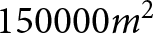 $150000 m^2$, supporting that MFP is able to separate several continuous, noisy sources from each other and therefore provide information that can complement glacial hydrological modelling. Both approaches have particular strengths: beamforming allows a detailed insight into the relationship between seismic sources on the glacier surface and diurnal glacial melt cycles, whilst MFP provides the opportunity to trace the change of more subtle noise patterns and identify consistencies in these patterns related to turbulent subglacial streams. Combined with additional methods to track subglacial hydrology, such as GPR or seismic borehole measurements, future work may be extended to provide a stable three-dimensional imaging of the subglacial drainage system. The non-invasive, low-cost approach and continuous data from seismic nodes on a glacier motivate future glacial and geomorphological research to apply these cryoseismological methods to detect the complex behaviour of subglacial drainage networks.
Acknowledgements
The support of Mattia Gianini, Fayezurahman Azizi, Jamal Shokory, Theo Wolf, Marjolein Gevers, Louka Schulze-Rouat, Paul Dutoit, Brandon Finley, Laurene Ville, Faye Perchanok, David Soldini, Davide Mancini, Mathilde Bayens, Esteban Arcos, Fabian Walter and Aurélien Ballu during the fieldwork was indispensable for the success of this project.
GitHub Copilot was used during this work to improve Python code developed by the authors. The authors have reviewed all changes and improvements of the code and take full responsibility.
Eva Wolf has received funding from Horizon Europe MSCA Doctoral Network EnvSeis under grant agreement No. 101073148.
Ugo Nanni has received support from the Research Council of Norway through the projects MAMMAMIA (grant no. 301837) and SLIDE (no. 337228).
Data availability statement
The code and method used for the processing of seismic data with MFP can be freely accessed here: https://lecoinal.gricad-pages.univ-grenoble-alpes.fr/resolve/.
Appendix A. Beamforming window length
Effects of window length on time delay per station pair: We tested five window lengths between one and 32 seconds regarding the phase delay, variances and mean coherency. We are using stations ‘20821’ and ‘08670’ of array two; a similar pattern can be found for other station pairs. Subfigure A1a shows a 270 seconds window at 05:00 in the morning, assuming little subglacial discharge activity, and subfigure A1b shows 270 seconds at 14:00 midday, where subglacial and supraglacial melt are assumed to dominate the seismic signal.  $ \tau [s] $ are the phase delays with variances (grey bars), and
 $ \overline{c} $ are the mean coherency values between all stations of one array. The bottom plots show seismograms for station 20821 normalised by their maximum.

Figure A1 Long description
Two time-series plots each show phase delay estimation variations across five analysis window lengths: 2.048 s, 4.096 s, 8.192 s, 16.384 s and 32.768 s. The x-axis shows time in seconds, ranging from 0 to 270. The y-axis for the top five plots is labeled tau (phase delay) in seconds, ranging from -0.25 to 0.25. The second last plot shows the mean coherency values [c] between all stations of one array. The bottom plot in each part is labeled Norm., representing normalized signal amplitude. Part a and b show relatively unstable phase delay estimations at smaller window lengths. The longer the window length, the more stable are the phase delays, but variances per estimation increase. The normalized signal shows fluctuations corresponding to the phase delay variations. Part b includes one more pronounced seismic event and higher glacial discharge of the diurnal discharge cycle. The legend differentiates the time window lengths. Key features are the variances of tau (phase delay), explaning the trade off between detecting stable phase delays and smoothing the results too much.
Appendix B. Accumulated amplitude
Accumulated amplitude of the signal from the glacier surface for two days with different meteorological conditions. On the frequency bands below 10 Hz, the amplitude has a rather constant level throughout the day, whilst for frequency bands above 100 Hz, a strong diurnal noise variability shows up. The decrease in amplitude between the 24 hour time windows is a processing artefact.

Figure B1 Long description
Seven time-series graphs representing the accumulated seismic amplitude recorded on the glacier surface, as well as meteorological information from 23rd to 25th August. The first five graphs display accumulated amplitude per 10 minutes for frequency bands: 1-10 Hz, 10-20 Hz, 20-40 Hz, 40-100 Hz and 100-125 Hz. Each graph shows amplitude fluctuations, with notable maxima in all frequency bands during the highest diurnal temeprature or precipitation events. The sixth graph shows normalied amplitude with varying peaks and diurnal amplitude variations. The seventh graph presents water stage, turbidity, precipitation and temperature over time. The left y-axis shows water stage in meters, while the right y-axis shows turbidity in NTU, precipitation in mm and temperature in degrees Celsius. Water stage peaks with a short delay to the highest diurnal temperature record or during precipitation events, coinciding with increased turbidity. The graphs illustrate relationships between diurnal seismic signal variations on different frequency bands and environmental changes.
Accumulated amplitude of the signal from the terminus of the glacier for two days with different meteorological conditions. Similar behaviour as in Figure B1 is found, except that in the lower frequency bands, the signal is less amplified.

Figure B2 Long description
Seven time-series graphs representing the seismic amplitude recorded at the glacial terminus, as well as meteorological information from 23rd to 25th August. The first five graphs display accumulated amplitude per 10 minutes for frequency bands: 1-10 Hz, 10-20 Hz, 20-40 Hz, 40-100 Hz and 100-125 Hz. Each graph shows amplitude fluctuations, with notable maxima in all frequency bands during the highest diurnal temperature or precipitation events. The sixth graph shows normalized amplitude with varying peaks and diurnal amplitude variations. The seventh graph presents water stage, turbidity, precipitation and temperature over time. The left y-axis shows water stage in meters, while the right y-axis shows turbidity in NTU, precipitation in mm and temperature in degrees Celsius. Water stage peaks with a short delay to the highest diurnal temperature record or during precipitation events, coinciding with increased turbidity. The graphs illustrate relationships between diurnal seismic signal variations on different frequency bands and environmental changes.
Appendix C. Beamforming small array
Comparison of the beamforming calculations for different array sizes. In Figure C1a, the pink markers show the selected stations for the repeated calculations using a smaller array aperture. Figure C1b presents the calculations for the big array in subfigure a1 as well as the calculations for the smaller, reduced array in subfigure a1.1, as well as their corresponding probability distributions. Whether the smaller or bigger array is used does influence the back azimuth and velocity calculations only very minor.

Figure C1 Long description
Subfigure a shows a big and a small version of seismic array configuration and associated time-series of back azimuth and apparent velocities recorded over 24 hours starting on 22nd August at 19:00 UTC. The top section shows a georeferenced map with triangle markers in white indicating seismic sensor positions of the original array, as well as pink triangles indicating the size of a smaller array to test the effect of array size on the beamforming results. A line connecting two markers is labeled 70 m, another one is labeled 35 m, indicating the spacing between different sensors. The scatter plots below show the beamforming results of the big (a1) and small (a1.1) Array. Data points are colored according to apparent velocity in km/s, with a shared color scale ranging from 1 to 10 km/s shown at the top of the figure. A probability density function panel to the right, labeled b1 and b1.1, shows the distribution of back azimuth values over 24 hours, with a visible peak concentrated between approximately 90 and 135 degrees. Subfigure c shows the normalised seismic amplitude of Station 20821. The trace is filtered between 3 to 7 Hz. Elevated amplitude bursts are visible at several intervals across the time window, with the largest excursions occurring near at 06:00 and again near at 12:00, along with diurnal variations of general signal intensity. The bottom section shows hydrologic variables plotted together over the same coordinated universal time x-axis. The left y-axis is labeled water stage in meters, ranging from approximately 0 to 0.3. The right y-axis shows values for precipitation in millimeters, turbidity in NTU and temperature in degrees Celsius. Water stage shows a gradual rise beginning near at 06:00 and peaking near at 13:00 before declining. Turbidity and temperature traces show corresponding increases during the same interval. This figure shows that the array size has little influence on the results presented.
Appendix D. Beamforming higher frequency band
Beamforming results for the frequency band of 20–40 Hz, showing the distribution of back azimuth and velocities. Sections b1–b3 show the probability density function of the values. Below, similar to Figure 3, a seismic trace and meteorological data are displayed in subfigures c and d. The detected back azimuths of this frequency band, which is associated with bedload transport, are similar to those on the lower frequency band of 3–7 Hz associated with turbulent stream signal. The most frequent detected velocities range around  ${\sim 1650 \ m s^{-1}}$.

Figure D1 Long description
The histogram on top of the figure shows the distribution of apparent velocity values labeled ′Vel. [km/s]′ with peaks around 2.5 km/s, showing the color code used in the subfigures below. Subfigures a1 to a3 display scatter plots for Arrays 1, 2 and 3, respectively, with back azimuth (BAZ) on the vertical axis and time on the horizontal axis. Array 1 and 2 show dense back azimuth detections between 90 and 180 degrees, while Array 3 shows a many detections between 180 and 270 degrees. Marginal plots next to each scatter plot show probability density functions (PDFs) with peaks corresponding to the dominant BAZ ranges. Subfigure c presents normalised seismic amplitude for ′Station 20821′, filtered at 20-40 Hz, showing increased amplitude coinciding with rising environmental factors. Subfigure d displays a multi-line time series with water stage, turbidity, precipitation and temperature over the same time window. The figure demonstrates the choice of frequency band for the beamforming analysis, as for higher frequency bands, the back azimuth variations do follow the hydrological variaitons less closely.
Appendix E. MFP vertical resolution
The vertical perspective of our area of interest on Glacier d’Otemma 23rd August. The upper black line marks the glacier surface, whilst the lower black line marks the beginning of the bedrock. The white points represent the starting points which we used for the synthetic sources with MFP. We set their elevation to the elevation of the bedrock of the glacier, so in this profile view, some points seem to be in the air because they are located further away or closer in the UTM North dimension. The noise sources are mostly identified on the surface of the glacier or even above. This is likely related to the processing of waves for which the glacier thickness corresponds to approximately half of a wavelength of 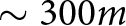 $\sim 300 m$, as explained in the discussion.

Figure E1 Long description
This figure shows the vertical source distribution of the MFP results on 23rd August. The black lines show the upper and the lower boundary of the glacier. A vertical color bar at the right shows source density between 0 and 0.0008. A legend to the right lists symbols shown in the glacier profile: high accuracy estimations, seismic sensors, starting points and bedrock. Seismic sensors are represented by grey trinagles. Starting points for the MFP algorithm are shown as small white circles. The bedrock underneath the glacier is represented by the grey area. Within the plot area, many high accuracy estimations, shown by red dots, are are clustering near the glacier surface. At around 379100 m East, a light vertical source density cloud is seen in the glacier profile. Most intense sources densities are nevertheless detected close to the glacier surface.
Appendix F. Meteorological and hydrological data
Seismic activity at the glacial terminus, glacier runoff, turbidity and meteorological data for the summer season of 2024 for Glacier d’Otemma. We observe a peak plateau in the daily water stage of the subglacial stream around the end of August, matching the time when the subglacial channel system detected with MFP suggests efficient channelisation (Figure 6i).

Figure F1 Long description
Spectrogram showing seismic power across frequencies for the full summer season of 2024 at the terminus of Glacier d’Otemma. The horizontal axis shows dates from 16th June to 31st August. The vertical axis shows the frequency [Hz] in logarithmic scale from 1 to 100. The color bar above the spectorgramm shows the color code for seismic power in decibel ranging between -180 and -150. Per day, we see the increase in seismic power across the full frequency range, with an increasing effect intensity towards the end of the season. During rainfall events, the seismic energy rises strongly over the full frequency range. Subfigure b shows the water level time series from 29th July to 31st August. Subfigure c shows the turbidity time series in the same time range. Subfigure d shows temperature and precipitation time series from 16th June to 31st August.
Appendix G. MFP with simulated data
Synthetic tests to evaluate the effect of seismic station configuration: We produced random seismic noise for both seismic station configurations (grid-shaped network versus three triangular arrays) as well as a 5 Hz signal, emitted repeatedly at random time intervals around half a second for three plausible source locations (red crosses) at the glacier bed. The propagation from the source to the stations is at the velocity of  ${\sim 1800 \ m s^{-1}}$. Subfigure G1a and G1b show the source distribution for only random noise signal, subfigure G1c and G1d show the source distribution for only signal and subfigure G1e and G1f show the source distribution for synthetic data composed of random noise and signal. The seismic station configuration has only very minor influence on the identified patterns, and does not affect the interpretation of large-scale patterns, as done in our analysis.

Figure G1 Long description
These figures show synthethic tests of the MFP algorithm for grid-shaped and triangular sensor configurations. Each figure contains red dots indicating high accuracy estimations, grey triangular markers for the seismic sensors, white circular markers for the starting points of the algorithm as well as red crosses showing where the synthetic source locations are. The vertical color bar to the right explains the color code for source density between 0 and 0.00002. Subfigure a and b show the source density estimation of the MFP algorithm when only random noise signal is processed. Here, the ‘sources’ are detected all around with the most pronounced source spot at the center of the area of interest. Subfigure c and d show the source locations deteced by MFP with only three, deep sources at the glacier bed emitting seismic signal. Those sources are well detected and can be distinguished from each other. Subfigure e and f show the results from the MFP algorithm when both, random noise and signal from three deep sources are used. Here, nevertheless, MFP manages to find and separate the three sources from each other.
Synthetic random noise at three different frequency bands and both sensor configurations (grid-shaped network versus three triangular arrays): 5 Hz in subfigure G2a and G2b, 20 Hz in subfigure G2c and G2d and 100 Hz in subfigure G2e and G2f. The MPF technique merges the optimised source locations for all starting points into a source density. In the case of random noise, the MPF source estimation is close to the starting point, and the source density area around the starting point is smaller for higher frequencies (Nanni and others, Reference Nanni, Roux, Gimbert and Lecointre2022).

Figure G2 Long description
This figure shows six source density maps of the MFP algorithm when only processing synthetic seismic noise, on the left side for seismic sensors configured in a grid-shaped network, and on the right side for sensors set up in triangular arrays. The first row of subfigures shows results for 5 Hz synthethic seismic noise, the second row of subfigures shows results for 20 Hz synthetic seismic noise and the last row of subfigures shows the results for 100 Hz synthetic seismic noise. Each subfigure contains grey triangles, showing sensor positions, as well as white circles, showing the starting points of MFP processing. The color bar to the right of each subfigure shows the color code for the source density between 0 and 0.00002. These six figures show that with increasing frequencies, seismic noise will be detected closer to the starting points of the MFP algorithm. This effect does not change between the two sensor configurations, grid-shaped or triangular.
Appendix H. Pressurisation coefficient tests
Sensitivity of predicted flow paths to the assumed, spatially uniform pressurisation constant  $c$ in the hydraulic potential calculation (Shreve, Reference Shreve1972). Panels H1a, H1b, H1c and H1d show results for
 $c = 0.1$,
 $0.3$,
 $0.7$ and
 $1.0$, respectively. Increasing
 $c$ increases the relative contribution of the ice thickness term to the potential field and tends to straighten and focus the predicted flow-convergent zones. These maps are not hydrological models of the drainage network, but first-order guides to where subglacial water would be expected to concentrate under each assumed pressure ratio.

Figure H1 Long description
Four thematic maps are arranged in a two-by-two grid, each showing the use of a different value for the pressursation constant c to calculate the hydraulic potential. The top-left map shows results for c = 0.1, the top-right shows results for c = 0.3, the bottom-left shows results for c = 0.7 and the bottom-right shows results for c = 1.0. The legend at top of the figure explains the use of symbols in the maps. The color bar shows the color code of source density, with values ranging from 0 to 0.00002. The light grey triangles represent seismic nodes in the configuration from 22nd to 25th August. The second color bar explains the color code for the hydraulic potential with values ranging from 0 to 10.454. The hydraulic potential, represented by the blue lines of different intensity on the glacier, changes with different values of c. This comparison shows that for a values of c = 1, the hydraulic potential estimations match as close as possible our estimated subglacial channel positions from the MFP analysis (purple colored clusters).
Appendix I. MFP window length
Matched field processing: MFP results for 23rd August 2024, processed with a window length of 16 seconds. The resulting point density is less profound than for one second windows, as we have about one order of magnitude less estimations points (I1a). The densities are more gathering around the sensors, which is a less viable trend than for the higher resolution, where most estimations are found centred around the estimated subglacial channel location (I1b).

Figure I1 Long description
These two histograms and the map show the MFP results for the 23rd of August when using 16 seconds processing windows instead of one second processing windows. 16 seconds was the window length used for the beamforming analysis. The first histogram in subfigure a shows the distribution of MFP output values. The maximum number of observations are found for values between 0 and 0.1. The second histogram shows the distribution of phase velocity values with a maximum number of estimations around 1600 m/s. In subfigure b, the grey triangles represent the seismic sensor positions. The white circles mark the starting points for the MFP algorithm. Red dots show source locations of high accuracy. The map of source densities shows three main source clusters, of which two are positioned relatively close to the sensor positions. This figure shows that larger processing windows for the MFP algorithm lead, in our case, to less accurate source positions.
Appendix J. MFP frequency comparison
Comparison of dominant noise sources for nine different frequency bands between 1 and 21 Hz (24 hour windows) for 23rd August 2024. The higher the frequency, the more distributed and small-scale noise sources are identified.

Figure J1 Long description
The plots illustrate source density variations of the MFP analysis across frequency bands from 1 to 21 Hz. The color scale represents source density between 0 and 0.0002. The grey triangles represent the seismic sensor positions. The white circles mark the starting points for the MFP algorithm. These figures show that with increasing frequency, the source positions become more scattered across the area of interest and spots of high source density are smaller.
Appendix K. Beamforming errors
Error values for back azimuth derivations: Sections a1–a3 show the temporal variety of back azimuth values and their corresponding errors. Sections b1–b3 show the probability density function of the values. Below, similar to Figure 3, a seismic trace and meteorological data are displayed in subfigures c and d. The dominant back azimuths identified, which are oriented parallel to the direction of glacier flow, have lower variances than those perpendicular to the flow. Additionally, error values decrease throughout the day, whilst runoff from the glacier and temperatures are high, and are higher at night, when back azimuth values are themselves more diffuse.

Figure K1 Long description
The figure shows the back azimuth estimations from the beamforming analysis and its corresponding error values. Panels a1, a2 and a3 show time series of back azimuth estimations between 0 and 360 degree for Arrays 1, 2 and 3, respectively. The color scale represents back azimuth error in degrees, ranging from 0 to 10. Panels b1, b2 and b3 show distributions of back azimuth values for each array over 24 hours. Panel c displays the seismic amplitude recorded at station 20821, showing the normalised amplitude filtered between 3-7 Hz. Panel d presents meteorological and hydrological data over the same time span. Multiple lines represent water stage (dark blue), turbidity (yellow), precipitation (light blue) and temperature (red). High back azimuth error values coincide with periods of low temperature and water stage. Error values of back azimuths are generally low for back azimuths around 45 and 225 degree, which are directions parallel to the glacier flow direction.
Error values of the apparent velocity time series: Sections a1–a3 show the temporal variety of apparent velocity values and their corresponding errors. Sections b1–b3 show the probability density function of the values. Below, similar to Figure 3, a seismic trace and meteorological data are displayed in subfigures c and d. The higher the velocity detected, the higher the error values become. Velocities and therefore error values are generally lower during the day whilst runoff from the glacier and temperatures are high.

Figure K2 Long description
The figure shows the apparent velocity estimations from the beamforming analysis and their corresponding error values. Panels a1, a2 and a3 show time series of apparent velocity estimations between 0 and 5000 m/s for Arrays 1, 2 and 3, respectively. The color scale represents the error of apparent velocity in m/s, ranging from 0 to 1000. Panels b1, b2 and b3 show distributions of apparent velocity values for each array over 24 hours. Panel c displays the seismic amplitude recorded at station 20821, showing the normalised amplitude filtered between 3-7 Hz. Panel d presents meteorological and hydrological data over the same time span. Multiple lines represent water stage (dark blue), turbidity (yellow), precipitation (light blue) and temperature (red). High apparent velocity error values coincide with periods of low temperature and water stage. Error values are generally higher for higher apparent velocity values.
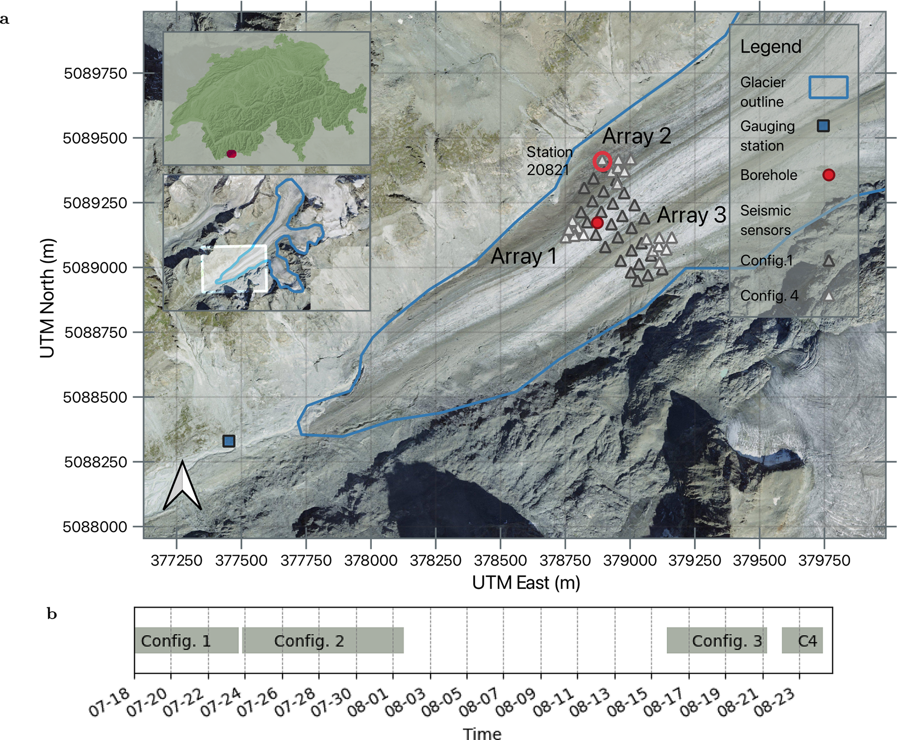
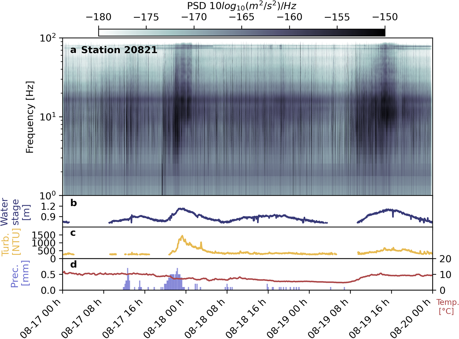
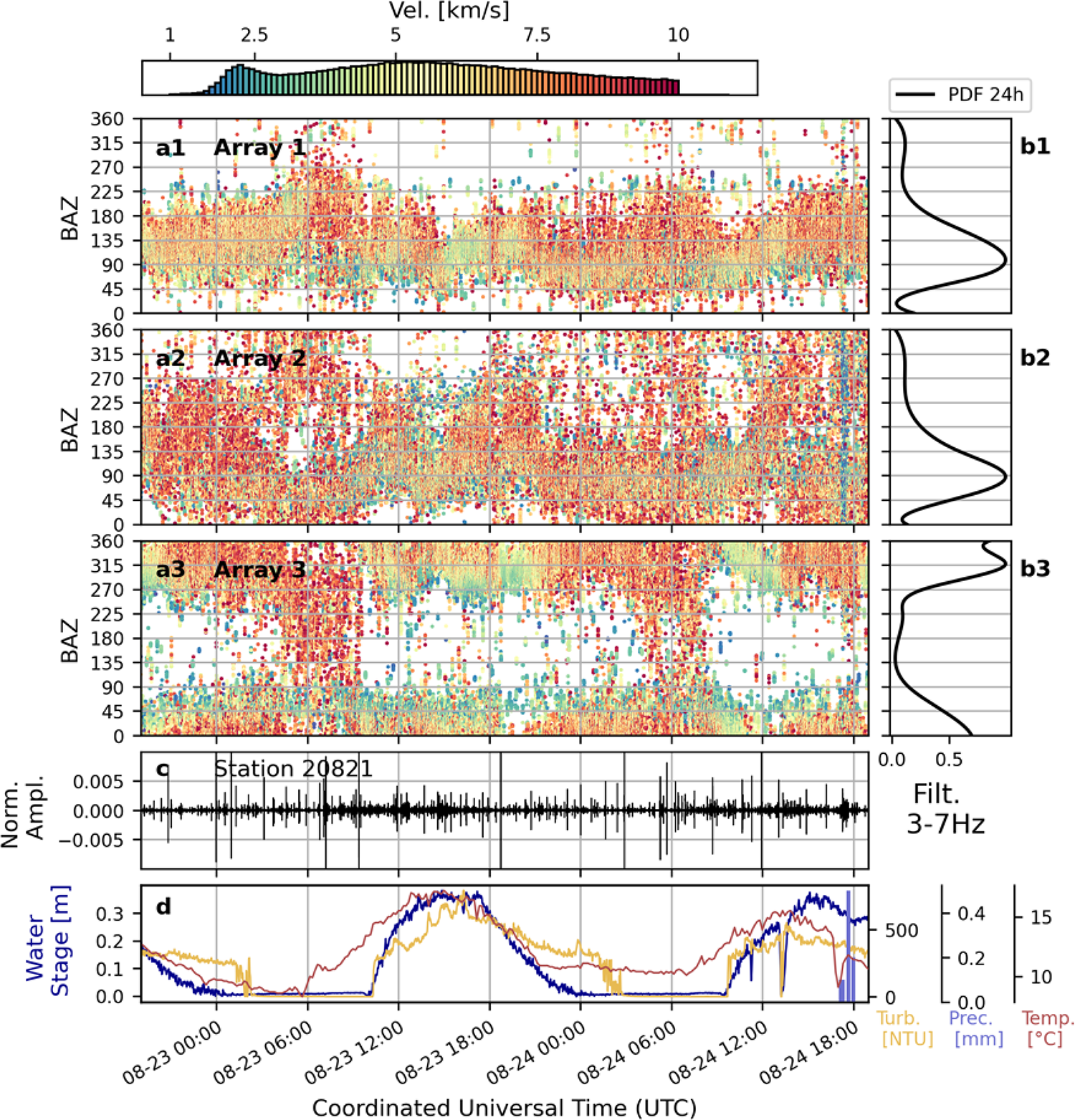
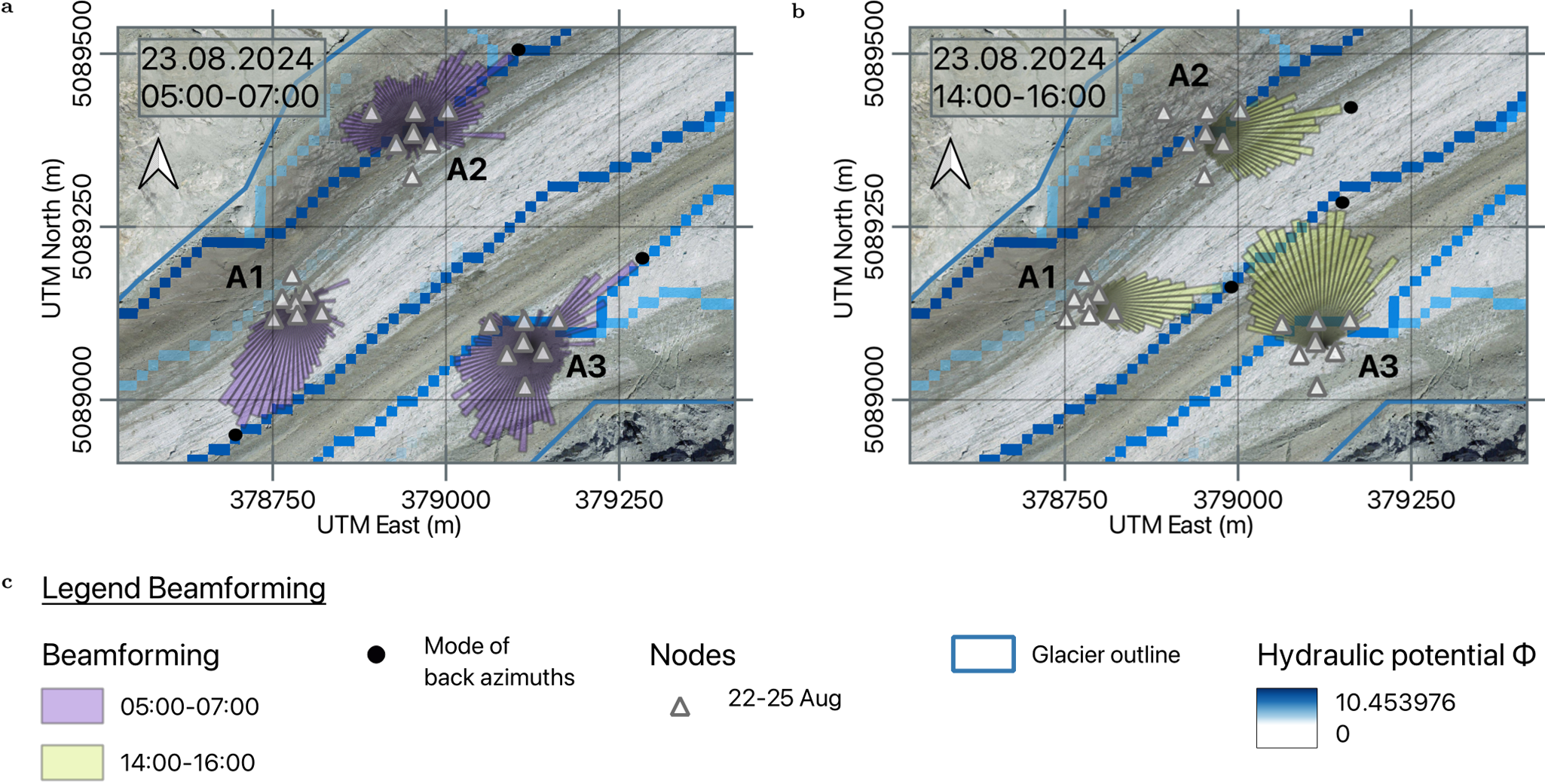
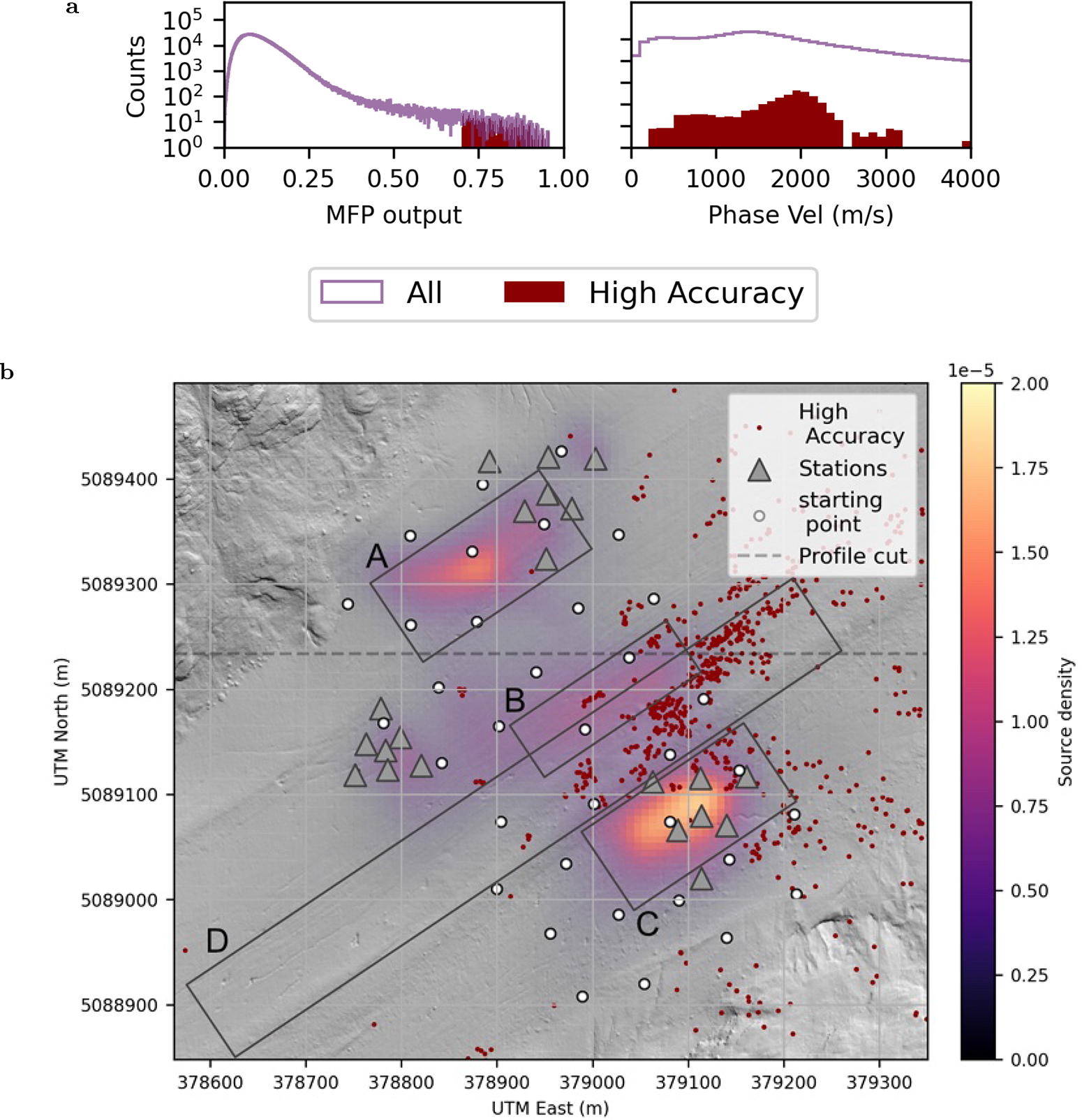
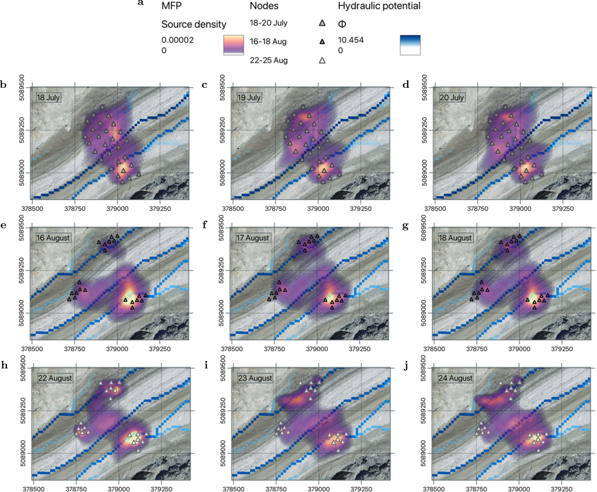
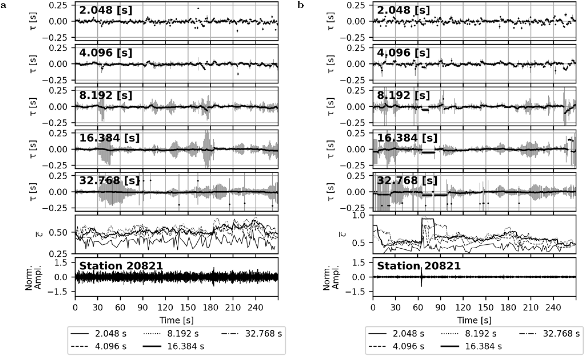


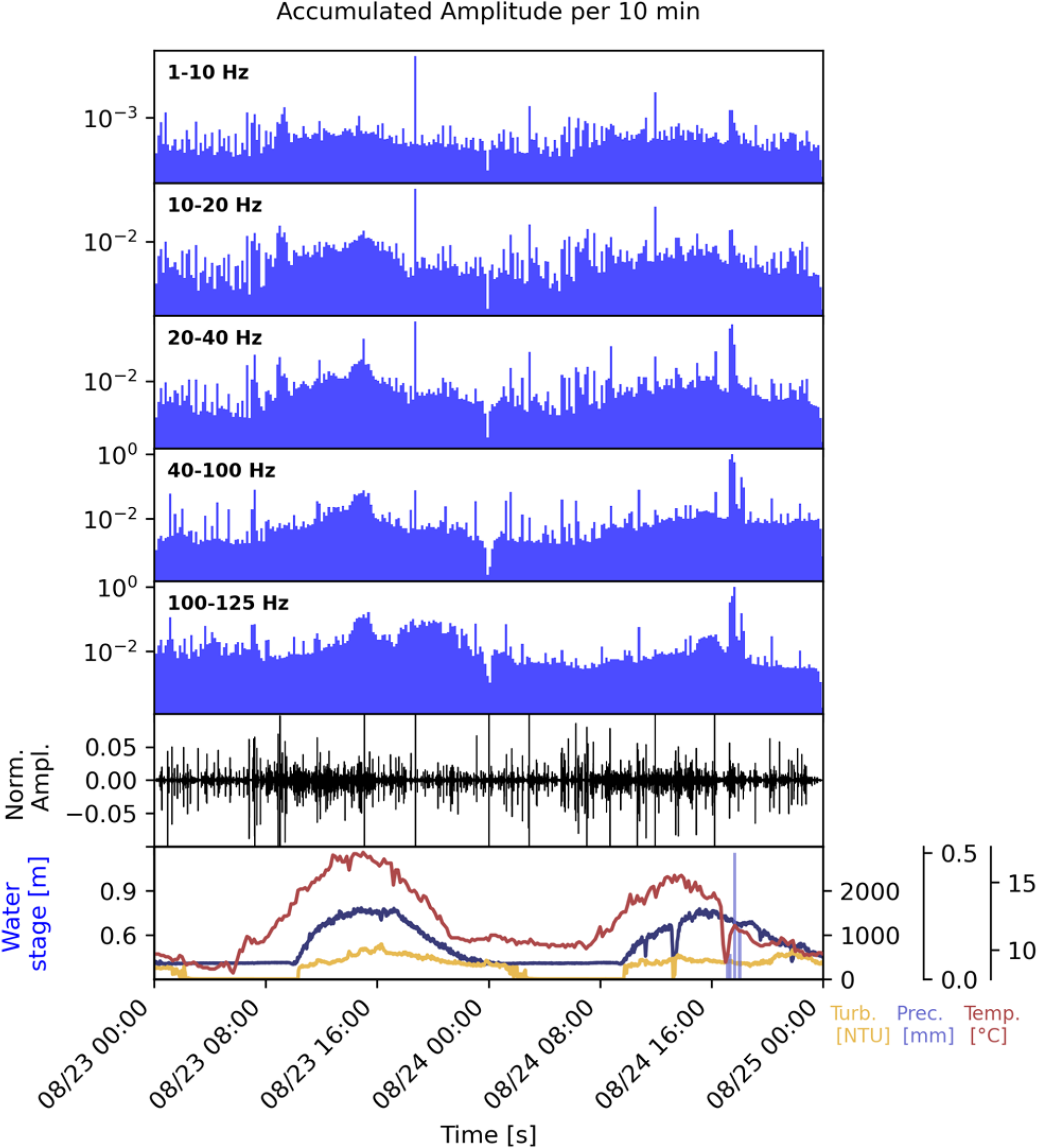
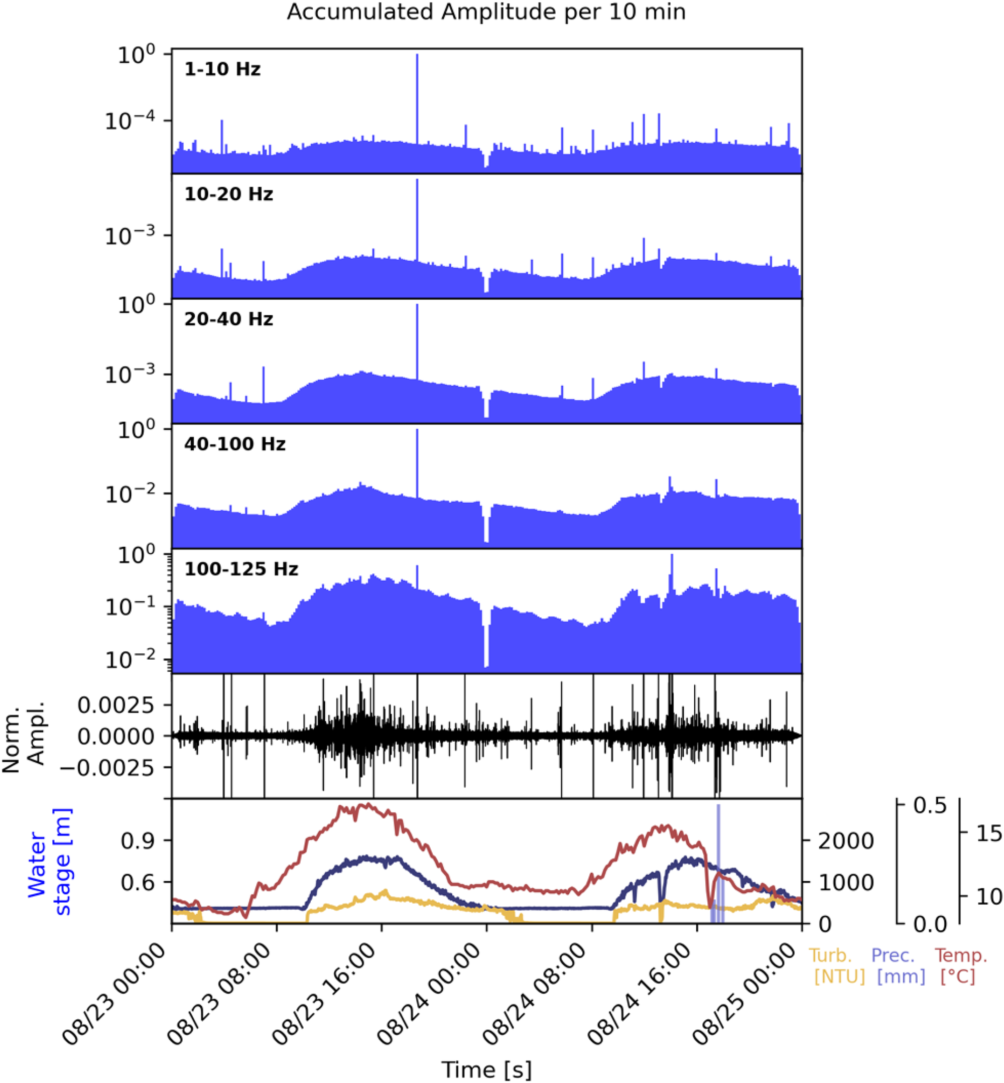
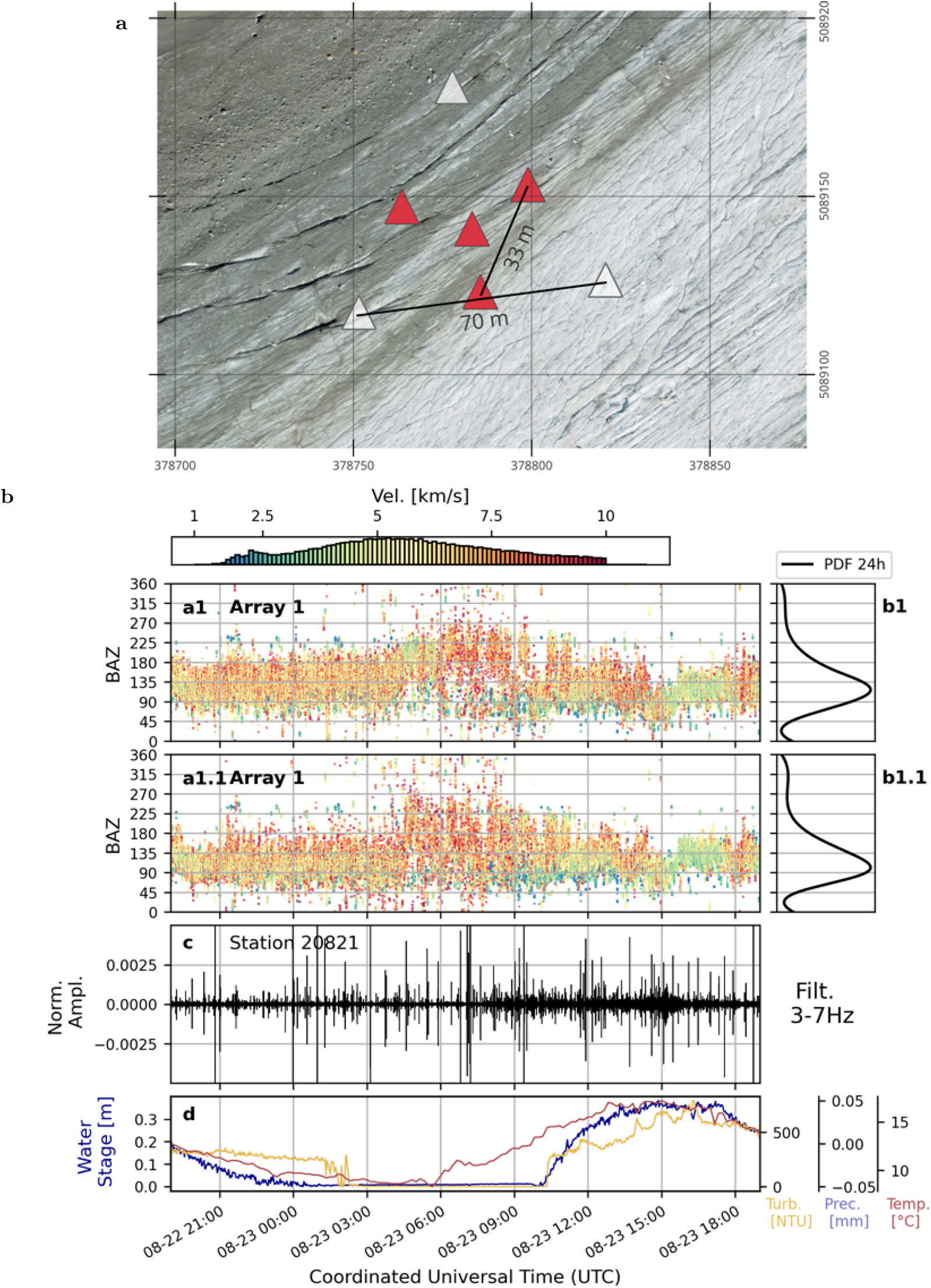
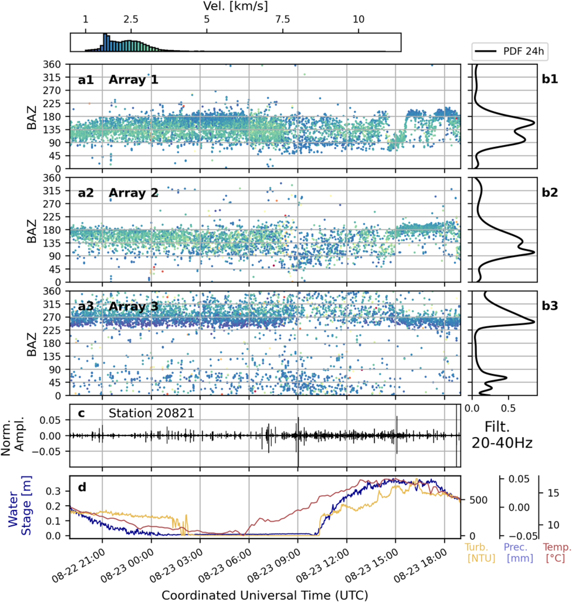

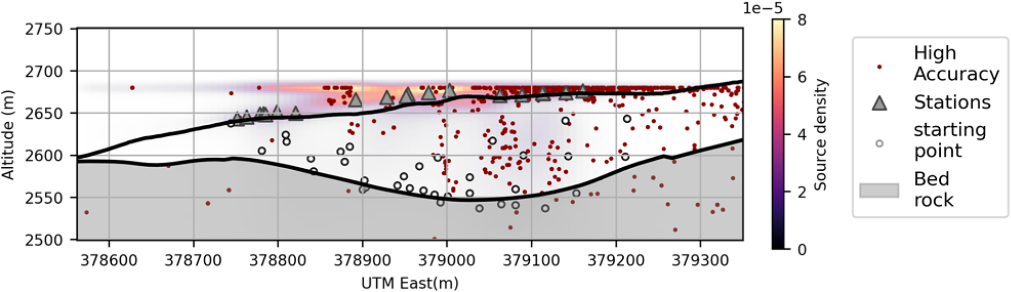

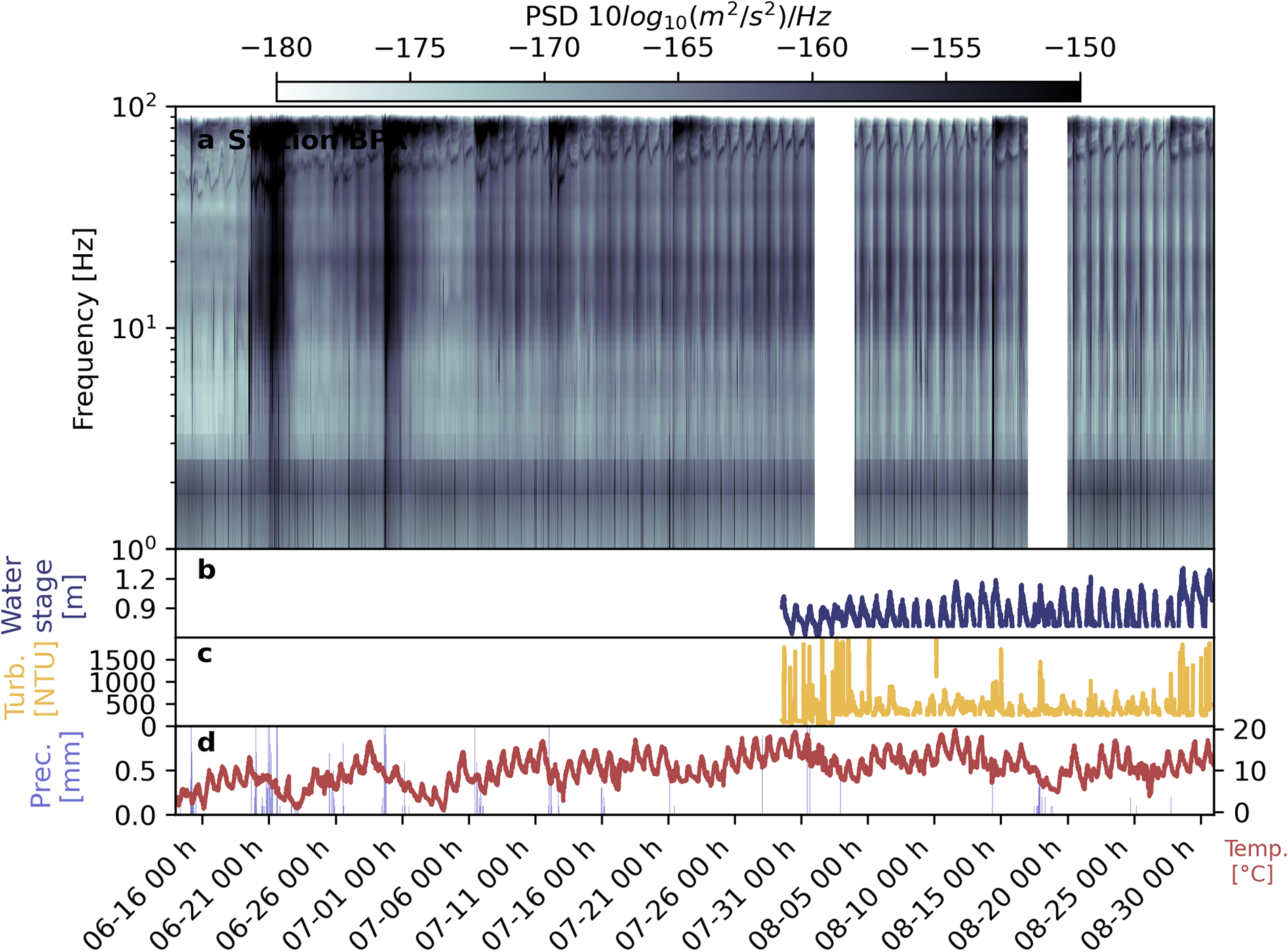
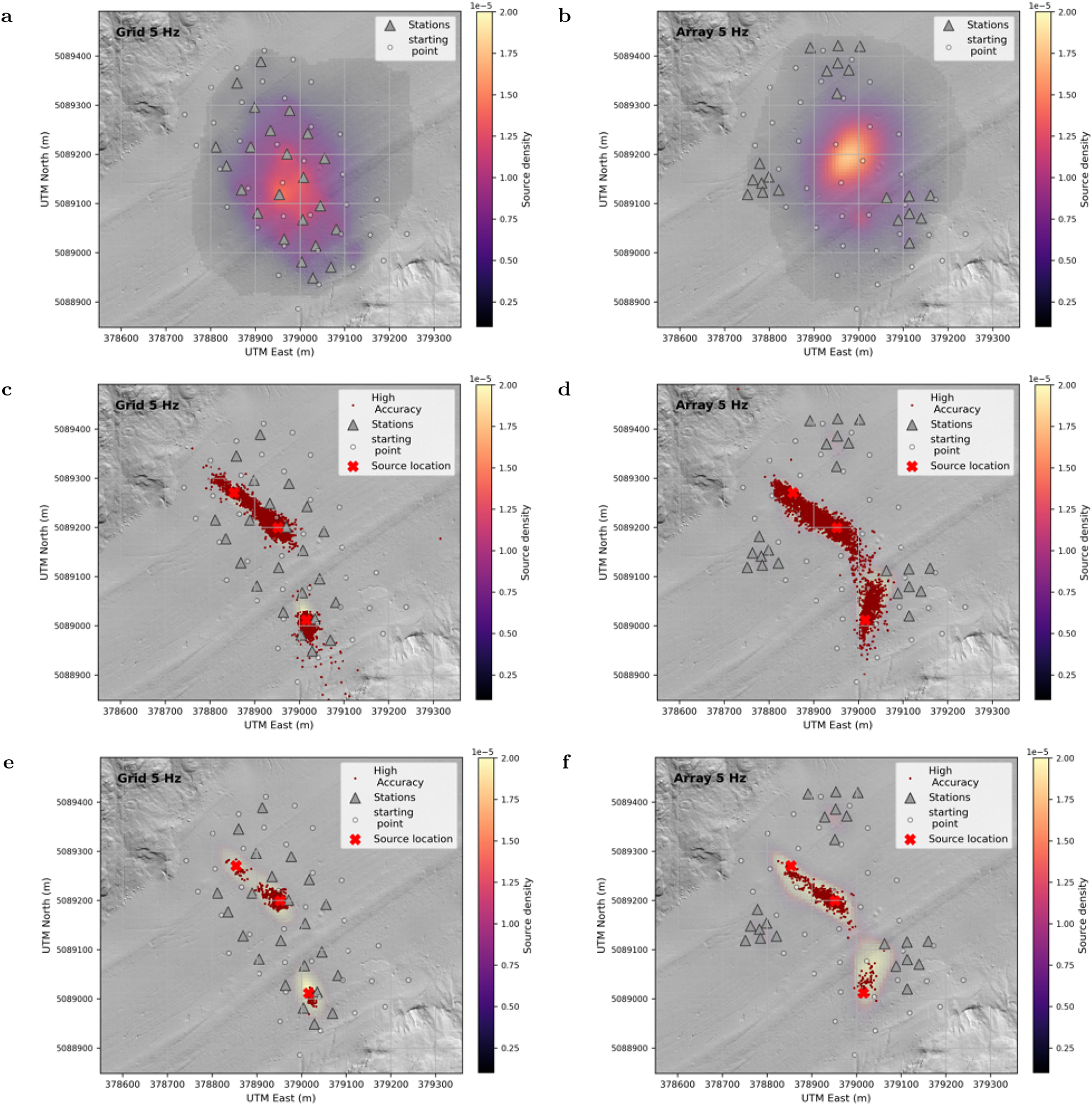

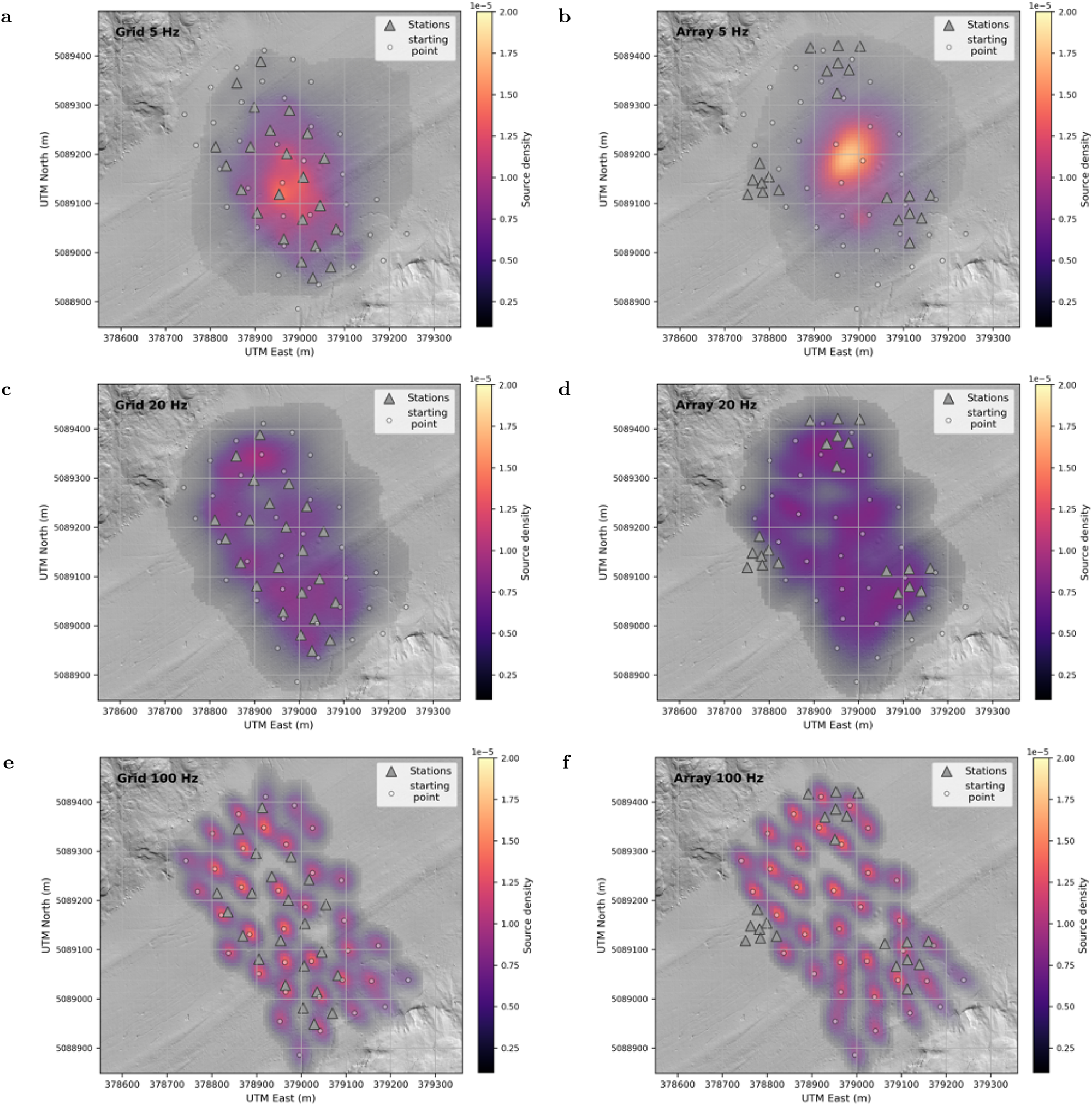
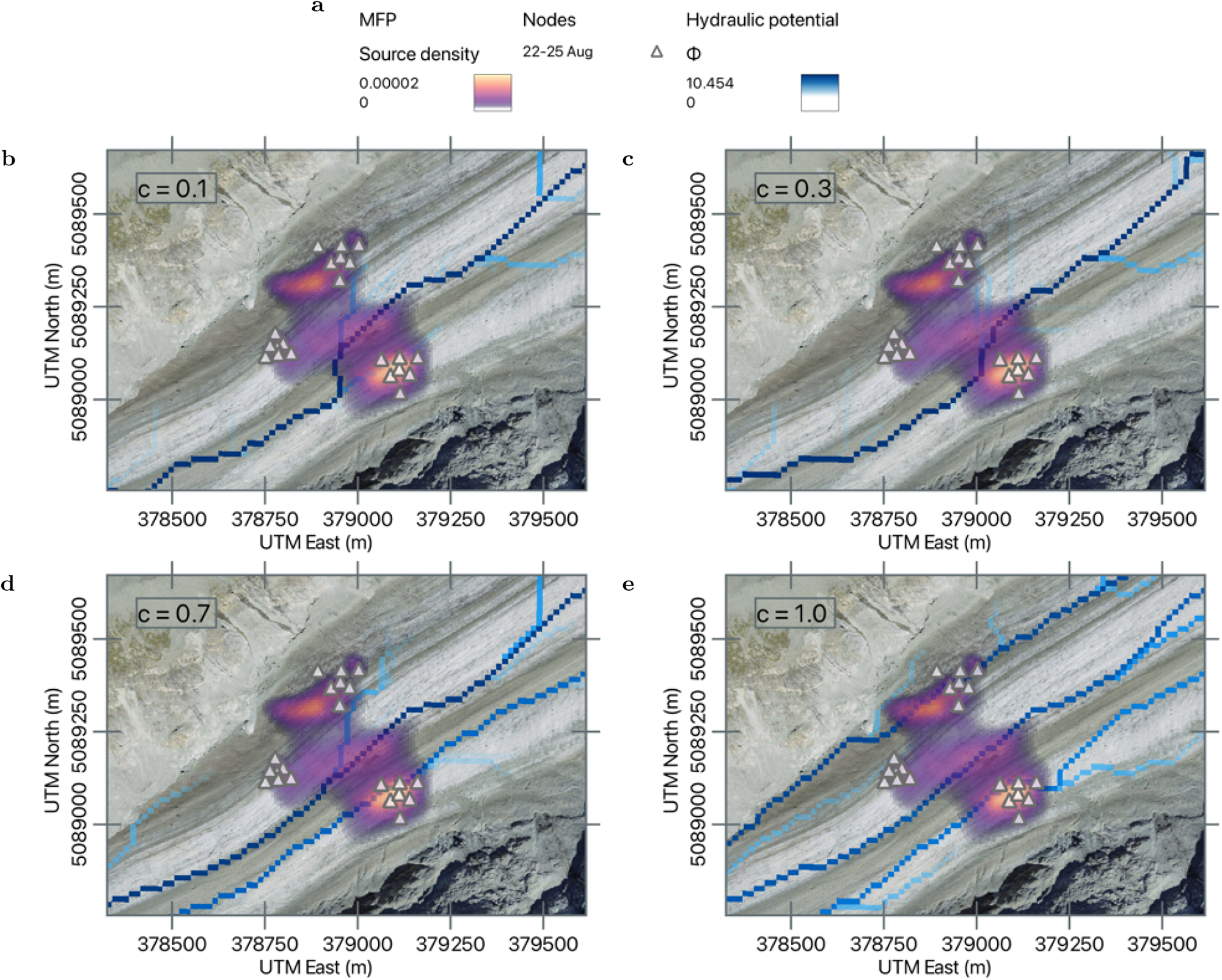


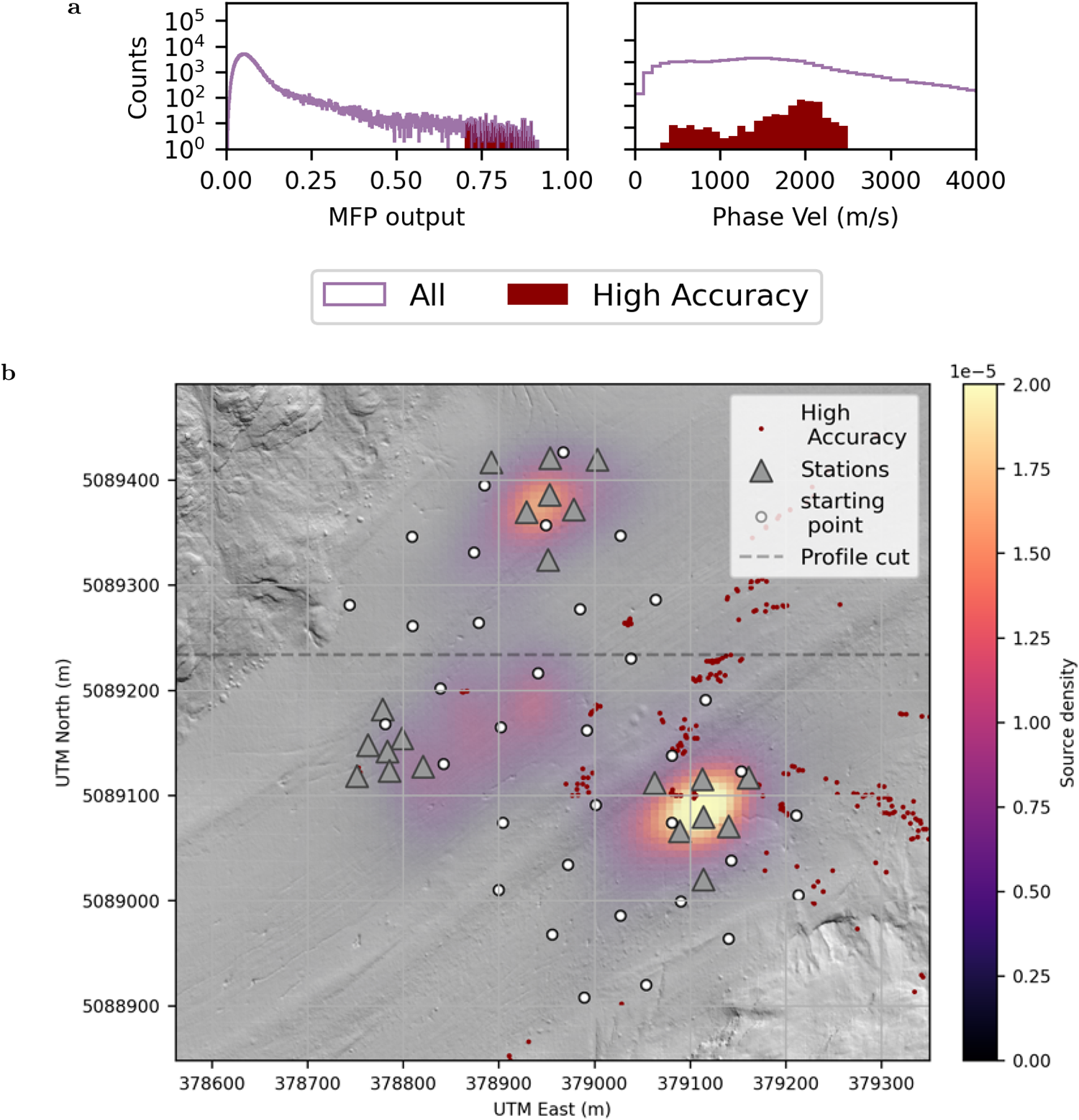
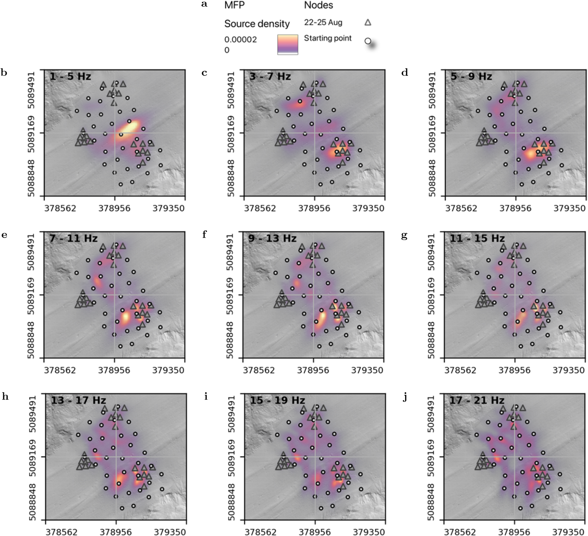
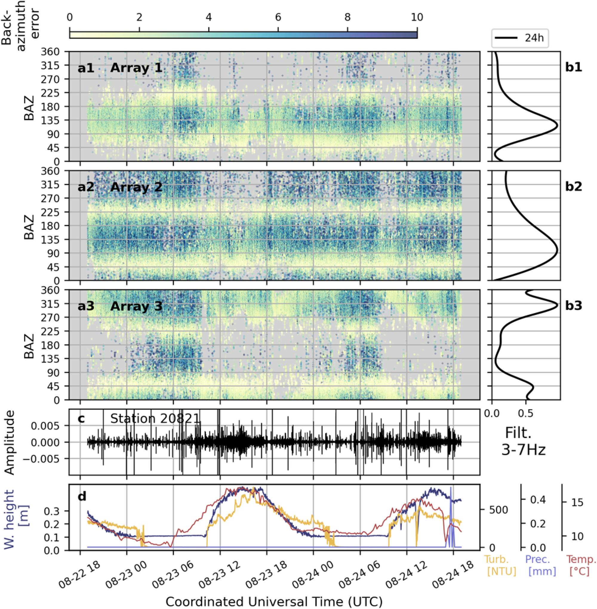
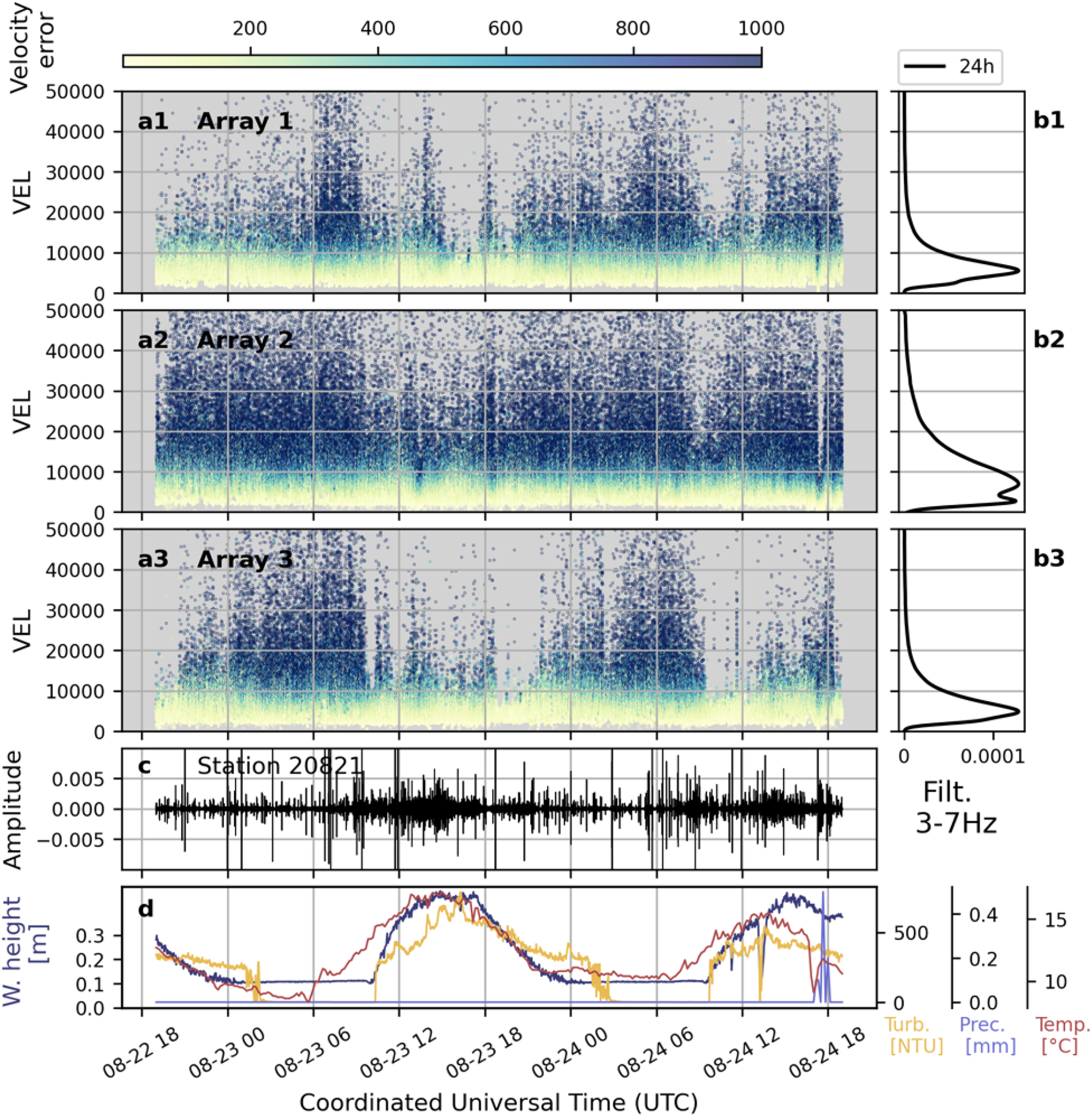

 Open access

