1. Introduction
Prediction of laminar–turbulent transition for supersonic or hypersonic boundary layers is of practical importance for high-speed aircraft designs due to its direct relevance to drag, heat transfer and flow separation (Fedorov Reference Fedorov2011; Zhong & Wang Reference Zhong and Wang2012). For low environmental perturbations, which are often the case in flight conditions, boundary-layer transition follows a natural route (Kachanov Reference Kachanov1994), for which four phases, i.e. the receptivity, linear instability, nonlinear breakdown and turbulence, appear in sequence. As to the first phase, receptivity is associated with the excitation of normal instability modes, including the first-, second- and higher-order Mack modes (Mack Reference Mack1987), by external perturbations such as free-stream acoustic, vortical and entropy disturbances. For supersonic boundary layers with smooth surfaces, two distinguished receptivity regimes may operate depending on the instability property of the excited normal modes. As pointed out by Smith (Reference Smith1989), only the first modes with oblique wave angles  $\varTheta >\sqrt {M^{2}-1}$ belong to the viscous nature, while the first modes with
 $\varTheta <\sqrt {M^{2}-1}$ and all the higher-order modes are inviscid, where
 $M$ denotes the oncoming Mach number. The receptivity of the inviscid modes is described theoretically by synchronisation mechanisms (Fedorov & Khokhlov Reference Fedorov and Khokhlov1991, Reference Fedorov and Khokhlov2001; Fedorov Reference Fedorov2003a), which include three types: (i) in the leading-edge vicinity, modes
 $F$ and
 $S$, two distinguished eigensolutions of the boundary-layer profiles, are synchronised with the free-stream fast and slow acoustic waves with phase speeds
 $c=1+1/M$ and
 $1-1/M$, respectively, (ii) at a downstream station, mode
 $F$ is synchronised with the external entropy/vortical wave with phase speed
 $c=1$ and (iii) near the lower-branch neutral position of the second Mack mode, modes
 $F$ and
 $S$ are synchronised, leading to the discrete spectrum branching. Such mechanisms were confirmed by direct numerical simulations (DNSs) of Ma & Zhong (Reference Ma and Zhong2003a, Reference Ma and ZhongReference Ma and Zhong2005), and agree with the experimental measurements of Maslov et al. (Reference Maslov, Shiplyuk, Sidorenko and Arnal2001) for small oblique angles
 $\varTheta$. For the viscous first modes with
 $\varTheta >\sqrt {M^{2}-1}$, Ricco & Wu (Reference Ricco and Wu2007) and Goldstein & Ricco (Reference Goldstein and Ricco2018) pointed out that the receptivity process is somewhat similar to the leading-edge receptivity of the Tollmien–Schlichting (T–S) wave in incompressible boundary layers (Goldstein Reference Goldstein1983). Additionally, there may be more regimes for the generation of viscous first modes, such as the interaction between a sound wave and a vortical wave (Wu Reference Wu1999) and the interaction between two sound waves (Hernández & Wu Reference Hernández and Wu2019). The second phase is associated with the exponential growth of normal instability modes, which is described by the linear stability theory (LST). The growth rate of the normal modes can be obtained by solving numerically the compressible Orr–Sommerfeld (O–S) equations, which have been studied extensively for several decades, such as Mack (Reference Mack1987) and Malik (Reference Malik1990). Note that the compressible O–S equations are also referred to as the Lees–Lin equations (Lees & Lin Reference Lees and Lin1946). When the amplitudes of the instability modes have been accumulated to finite values, their nonlinear interactions would lead to the rapid distortion of the mean flow and the excitation of more perturbations in a short distance, which eventually leads to breakdown of the laminar flow and emergence of turbulence. A comprehensive review of the nonlinear theories can be found in Wu (Reference Wu2019). Because the linear evolution of the instability modes occupies most of the laminar phase, an e-N transition prediction approach was developed based on LST (Smith Reference Smith1956; Jaffe, Okamura & Smith Reference Jaffe, Okamura and Smith1970), in which the threshold of the transition onset is characterised by an empirical factor
 $N$.
If there exist surface imperfections on high-speed vehicles, such as roughness elements, steps, gaps and corners, transition would be influenced by the following two mechanisms.
First, the imperfections can interact with free-stream perturbations and excite instability modes locally, which is referred to as local receptivity. The local receptivity of the viscous first modes due to sound–roughness interaction is essentially the same as that of the T–S modes in the incompressible and subsonic regimes (Ruban Reference Ruban1984; Goldstein Reference Goldstein1985). However, as revealed by Liu, Dong & Wu (Reference Liu, Dong and Wu2020) for localised roughness and Hernández & Wu (Reference Hernández and Wu2019) for distributed roughness, an even stronger receptivity may appear when the free-stream acoustic wave is at a particular incident angle such that the acoustic-driven Stokes layer has a large streamwise perturbation velocity in the near-wall region. On the other hand, the local receptivity of the inviscid Mack modes is rather different from that of the viscous modes because the wavelength of the former is as short as the local boundary-layer thickness. Using the biorthogonal eigenvalue system as in Tumin & Fedorov (Reference Tumin and Fedorov1983) and Tumin (Reference Tumin2007), Fedorov (Reference Fedorov2003b) developed a finite-Reynolds-number theory to describe quantitatively the receptivity efficiency due to sound–roughness interaction. An asymptotic theory was recently developed by Dong, Liu & Wu (Reference Dong, Liu and Wu2020). It was found that for a roughness element with a height of  $O(R^{-1/3}\delta )$ and a width of
 $O(\delta )$, where
 $R$ is the Reynolds number based on the local boundary-layer thickness
 $\delta$, the leading-order receptivity is due to the distortion of the acoustic signature by the curved wall, while the second order is contributed by the interactions between the roughness-induced mean-flow distortion and the acoustic signature.
Second, the imperfection would scatter the oncoming instability mode, which leads to a quantitative change of its amplitude in the downstream limit. This problem was extensively studied by simulations and experiments for the motivation of laminar-flow control, and was described mathematically by local scattering theory (Wu & Dong Reference Wu and Dong2016b) in subsonic boundary layers. In that paper, the imperfection was chosen to be an isolated roughness element, and the scattering effect was quantified by a transmission coefficient,  $\mathscr {T}$, defined as the ratio of the asymptotic amplitude downstream of the roughness to that upstream. It was also suggested that the
 $N$-factor in the e-N transition prediction approach should undergo an increment
 $\Delta N=\ln (|\mathscr {T}|)$ due to the scattering effect. Because the instability in subsonic boundary layers is of a viscous T–S nature, the theory of Wu & Dong (Reference Wu and Dong2016b) was based on the triple-deck formalism (Stewartson Reference Stewartson1969; Messiter Reference Messiter1970; Smith Reference Smith1973). Such a theory was later extended to other types of imperfections (Dong & Zhang Reference Dong and Zhang2018; Zhao & Dong Reference Zhao and Dong2020), and also to transonic boundary layers (Dong Reference Dong2020). However, the inviscid Mack modes in supersonic or hypersonic boundary layers do not satisfy the triple-deck scaling, and so their scattering needs to be described by a completely different theory.
For supersonic or hypersonic wind-tunnel experiments, whether roughness elements promote or delay transition depends on a comprehensive effect of the two aforementioned regimes. As reviewed by Schneider (Reference Schneider2008), most of the early experiments reported that the effect of sizable roughness is to move transition forward, with the amount of forward movement increasing with the roughness height. However, a few experiments did find the delay of transition by two-dimensional (2-D) roughness elements in some circumstances (Holloway & Sterrett Reference Holloway and Sterrett1964; Fujii Reference Fujii2006). In order to reveal the intrinsic mechanism of the effect of roughness on transition, a number of numerical works were carried out by introducing only the oncoming Mack modes as the inflow perturbations, such that the local receptivity regime is excluded. Marxen, Iaccarino & Shaqfeh (Reference Marxen, Iaccarino and Shaqfeh2010) performed DNS to study the impact of 2-D roughness elements on oncoming first and second Mack modes in a Mach 4.8 boundary layer. It was found that the 2-D roughness behaves as disturbance amplifier with a limited frequency band. Duan, Wang & Zhong (Reference Duan, Wang and Zhong2013) and Fong, Wang & Zhong (Reference Fong, Wang and Zhong2014, Reference Fong, Wang and Zhong2015b) simulated the same problem by increasing the oncoming Mach number to a hypersonic level, 5.92. Through case studies for different roughness locations, they concluded that the synchronisation frequency of modes  $F$ and
 $S$ (the third type of synchronisation mentioned in the first paragraph) acts as a critical frequency, above and below which the oncoming Mack modes are suppressed and enhanced, respectively. Based on this concept, Fong et al. (Reference Fong, Wang, Huang, Zhong, McKiernan, Figher and Schneider2015a) designed a roughness distribution, and the suppression of the second mode was confirmed by experiments conducted at the Boeing/AFOSR Mach 6 quiet wind tunnel at Purdue University.
So far, it is accepted that the synchronisation point of modes  $F$ and
 $S$ plays a critical role distinguishing the destabilising and stabilising effects of the roughness. However, the reason why the synchronisation point is so special is not yet understood. In order to address this issue, more systematic parametric studies are needed. The linear parabolic stability equation is one efficient candidate, but the aspect ratio (height to width) of the roughness has to be small (Park & Park Reference Park and Park2013, Reference Park and Park2016), because the scattering system is elliptic if the aspect ratio is of
 $O(1)$. In order to overcome this shortcoming, Zhao, Dong & Yang (Reference Zhao, Dong and Yang2019) utilised the so-called harmonic linearised Navier–Stokes (HLNS) approach, in which the elliptic nature of the scattering system is retained and the time advancing as in the DNS approach is avoided by performing Fourier transform with respect to time. Such a treatment reduces the scattering system to a high-dimensional linear equation system. The HLNS calculations were confirmed to be of high accuracy by comparing with the DNS data, and a systematic study of the scattering effect for different roughness sizes and oncoming-mode frequencies was provided. A few unexpected or unexplained phenomena were observed: (i) for the same frequency band, humps and indentations play the same stabilising or destabilising role, and the scattering effect of an indentation is weaker than that of a hump with the same size; (ii) the scattering effect increases with Reynolds number if the dimensionless roughness size is fixed; (iii) for humps with the same height that is moderate, changing their widths does not lead to an apparent change of the scattering effect. In order to explain these phenomena and probe the scattering mechanism at the synchronisation point, we will develop an asymptotic theory to describe this problem.
For analytical convenience, we will assume the roughness to be much lower and wider than the local boundary-layer thickness. At first glance, the wide-roughness assumption may be inappropriate, because it leads to the degeneration of the scattering process to the modification of the local growth rate of the Mack modes. However, as the unexpected phenomenon (iii) indicates, the scattering effect seems to be insensitive to the width of the roughness, and so such an asymptotic theory may also reveal the scattering mechanism for narrow-roughness configurations. Therefore, we borrow the terminology ‘scattering’ to describe the impact of the wide roughness on oncoming Mack modes in this paper, despite the fact that the length scales of the instability and the roughness do not match.
2. Mathematical description
2.1. Physical problem and asymptotic scalings
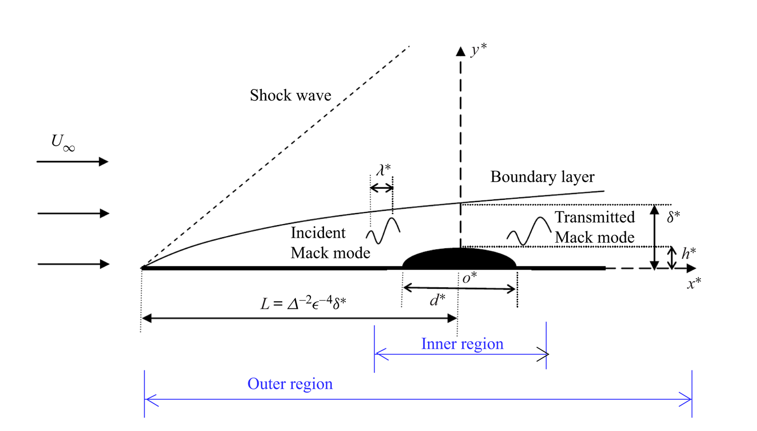
The physical model to be studied is a semi-infinite flat plate inserted into a supersonic/hypersonic uniform stream with a velocity  $U_\infty$, such that a viscous boundary layer and a weak oblique shock wave form on each side of the plate; see the sketch of the upper-half plane in figure 1. The fluid is assumed to be a perfect gas. The plate is taken to be isothermal, but the theory also applies to adiabatic walls. A roughness element with a height
 $h^{*}$ and width
 $d^{*}$ is located at a distance
 $L$ downstream of the leading edge. In what follows, we use the asterisk to represent dimensional quantities. We assume an oncoming inviscid Mack mode with a frequency
 $\omega ^{*}$ and a wavelength
 $\lambda ^{*}$ to propagate over the roughness, and the perturbation, after interacting with the roughness, is referred to as the transmitted Mack mode.
Sketch of the physical model.

The displacement thickness of the boundary layer at the roughness site,  $\delta ^{*}=\varDelta \sqrt {\nu _\infty L/U_\infty }$, is taken to be the characteristic length for normalisation, where
 $\nu _\infty$ is the kinematic viscosity of the oncoming stream and
 $\varDelta$ is a constant obtained from the compressible Blasius similarity solution. Note that
 $\varDelta$ increases with the oncoming Mach number, and is therefore much greater than 1 in the hypersonic regime. For instance,
 $\varDelta \approx 16.9(10.4)$ for a Mach 5.92(4.5) boundary layer with an adiabatic wall. The problem is described in the Cartesian coordinate system
 $(x^{*},y^{*},z^{*})$ with its origin at the lower centre of the roughness element, which is normalised as
 $(x,y,z)=(x^{*},y^{*},z^{*})/\delta ^{*}$. The velocity field
 $\boldsymbol {u}=(u,v,w)$, density
 $\rho$ and temperature
 $T$ are normalised by
 $U_\infty$,
 $\rho _\infty$ and
 $T_\infty$, respectively, where the subscript
 $\infty$ denotes the quantities of the oncoming stream. The pressure
 $p$ and time
 $t$ are normalised by
 $\rho _\infty U_\infty ^{2}$ and
 $\delta ^{*}/U_\infty$, respectively. The Reynolds and Mach numbers are taken to be
 $R=U_\infty \delta ^{*}/\nu _\infty =\varDelta \sqrt {U_\infty L/\nu _\infty }$ and
 $M=U_\infty /a_\infty$, respectively, where
 $a$ denotes the sound speed. In this paper, we take
 $R\gg 1$ and
 $M>1$. For simplicity, we introduce a small parameter
 \begin{equation} \epsilon=R^{{-}1/4}\ll 1. \end{equation}
The roughness is taken to be two-dimensional, whose height  $h^{*}$ and width
 $d^{*}$ are of
 $O(\epsilon \delta ^{*})$ and
 $O(\epsilon ^{-1}\delta ^{*})$, respectively. For an asymptotically large
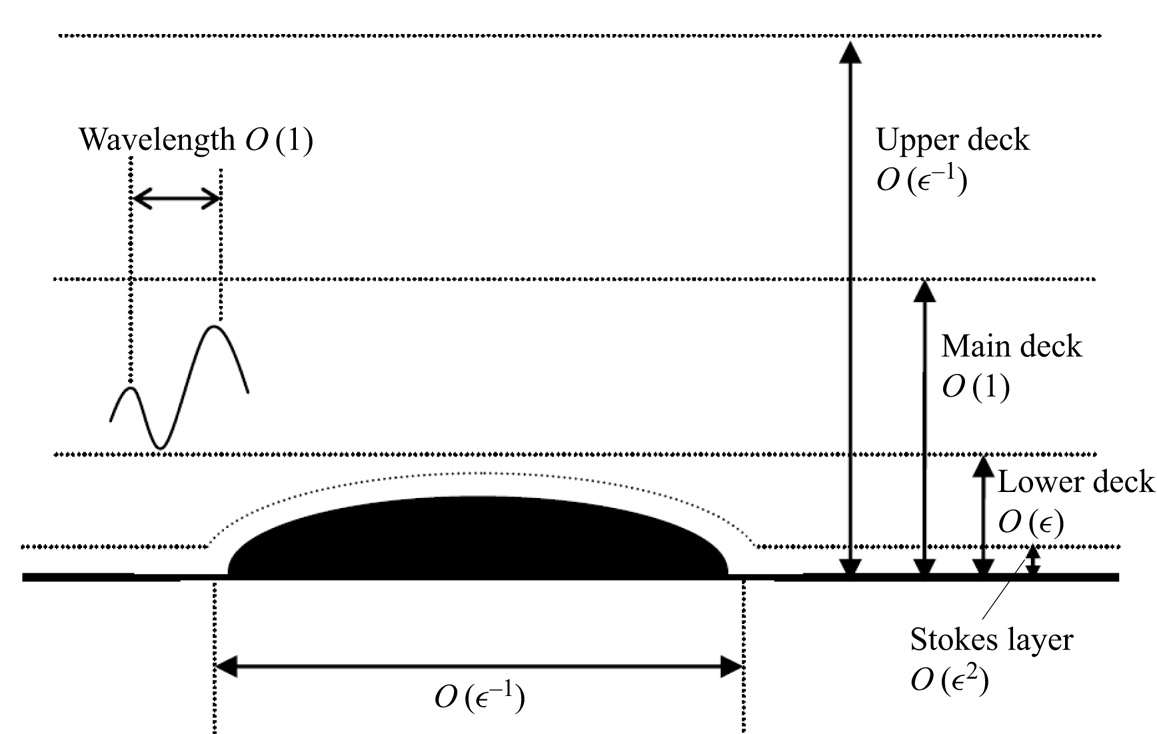
 $R$, a three-layered structure (including the lower, main and upper decks) appears in the transverse direction; see figure 2. Typically, the wavelength of the Mack mode
 $\lambda ^{*}$ is comparable to the local boundary-layer thickness
 $\delta ^{*}$, which is much shorter than the roughness width. In the transverse direction, the Mack mode exhibits a two-layered structure, i.e. an inviscid main deck in the bulk region where
 $y^{*}=O(\delta ^{*})$, and a viscous Stokes layer in the
 $O(\epsilon ^{2}\delta ^{*})$ vicinity of the wall. Note that if the Mack mode is quasi-neutral, a critical layer, at which the mean velocity is equal to its phase speed, would appear as another distinguished asymptotic layer, and calculating the main-deck solution requires a specific treatment as in Dong et al. (Reference Dong, Liu and Wu2020). However, for the majority of cases, the Mack mode is unstable with a complex phase speed, and so the critical layer is not needed. The neutral modes only appear in the case studies in § 4.4.4, and the numerical method to deal with the singularity is introduced there. Additionally, there exists another length scale
 $L=\varDelta ^{-2}\epsilon ^{-4}\delta ^{*}$, which is associated with the non-parallelism of the Blasius solution and is much greater than
 $\epsilon ^{-1}\delta ^{*}$.
Multi-scale structure of the inner region.

In summary, there are three length scales in the streamwise direction, i.e.  $(x,X,\bar x)=(x,\epsilon x,\varDelta ^{2}\epsilon ^{4} x)$, while four length scales appear in the transverse direction, i.e.
 $(\bar {y},y,Y,\bar {Y})=(\epsilon y,y,\epsilon ^{-1}y,\epsilon ^{-2}y)=O(1)$. In the streamwise direction, the regions where
 $X=O(1)$ and
 $\bar {x}=O(1)$ are referred to as the inner and outer regions, respectively, which are shown in figure 1. A clear demonstration of the asymptotic scalings in the inner region is shown in figure 2.
Note that the above scaling analysis is valid for all supersonic and hypersonic configurations, as long as the instability is the inviscid Mack mode. Therefore, the Mach number must satisfy  $M^{2}-1\gg R^{-2/9}$ (Ruban, Bernots & Kravtsova Reference Ruban, Bernots and Kravtsova2016; Dong Reference Dong2020), such that the transonic regime is excluded. On the other hand, there is no upper limit of
 $M$ in our theory. Admittedly, since the perfect-gas model is assumed, the quantitative results of our theory for extremely high Mach numbers may become inaccurate due to the high-temperature (real-gas) effect, including the excitation of the vibration energy of molecules and the chemical dissociations and reactions. However, for these extreme configurations, our theoretical framework can readily be applied if the real-gas model is added into the governing equations.
2.2. Governing equations
For a perfect gas with a constant ratio of specific heats  $\gamma$, the dimensionless Navier–Stokes (N–S) equations are (Zhao & Dong Reference Zhao and Dong2020)
 \begin{equation} \left.\begin{gathered} \displaystyle\frac{\partial \rho}{\partial t}+\boldsymbol{\nabla}\boldsymbol{\cdot} (\rho \boldsymbol{u})=0,\\ \rho\frac{\partial \boldsymbol{u}}{\partial t}+\rho(\boldsymbol{u}\boldsymbol{\cdot} \boldsymbol{\nabla})\boldsymbol{u}={-} \boldsymbol{\nabla} p+\frac{1}{R}\boldsymbol{\nabla}\boldsymbol{\cdot} (2\mu \boldsymbol{\mathsf{e}})+\frac{1}{R}\boldsymbol{\nabla}\left[\left({\mu_0}-\frac{2}{3}\mu\right)\boldsymbol{\nabla} \boldsymbol{\cdot}\boldsymbol{u}\right],\\ \rho\frac{\partial T}{\partial t}+ \rho(\boldsymbol{u}\boldsymbol{\cdot} \boldsymbol{\nabla})T=(\gamma-1)M^{2}\left[\frac{\partial p}{{\partial \bar{t}}}+(\boldsymbol{u} \boldsymbol{\cdot} \boldsymbol{\nabla})p\right]+ \frac{\boldsymbol{\nabla}\boldsymbol{\cdot}(\mu\boldsymbol{\nabla} T)}{{Pr}R}+ \frac{(\gamma-1)M^{2}\varPhi}{R},\\ \gamma M^{2} p=\rho T, \end{gathered}\right\}\end{equation}
where the strain rate tensor  $\boldsymbol{\mathsf{e}}$ and the dissipation function
 $\varPhi$ are expressed as
 \begin{equation} {\mathsf{e}}_{ij}=\frac{1}{2}\left(\frac{\partial u_i}{\partial x_j}+\frac{\partial u_j}{\partial x_i}\right),\quad \varPhi=2\mu\boldsymbol{\mathsf{e}}\boldsymbol{:}\boldsymbol{\mathsf{e}}+({\mu_0}-\tfrac{2}{3}\mu)( \boldsymbol{\nabla}\boldsymbol{\cdot}\boldsymbol{u})^{2}, \end{equation}
where  $Pr$ is the Prandtl number,
 $\mu =\mu (T)$ the dimensionless dynamic viscosity coefficient and
 $\mu _0=\mu _0^{*}/\mu _\infty$ is the dimensionless second viscosity. Note that the equation of state is slightly different from that in Zhao & Dong (Reference Zhao and Dong2020) due to the different definitions of the normalised pressure. Here, we choose Sutherland's viscosity law,
 $\mu (T)=(1+\bar {\mathcal {C}})T^{3/2}/(T+\bar {\mathcal {C}})$ with
 $\bar {\mathcal {C}}=110.4/T_\infty$, and take
 $\gamma = 1.4$,
 $Pr=0.72$ and
 $\mu _0=0$.
The instantaneous flow field is expressed as a superposition of the mean flow  $\bar{\boldsymbol\varphi}$ and the unsteady perturbation
 $\tilde {\boldsymbol\varphi}$,
 \begin{equation} {\boldsymbol\varphi}(x,y,z,t)=\bar{\boldsymbol\varphi}(x,y)+\tilde{\boldsymbol\varphi}(x,y,z,t), \end{equation}
where  ${\boldsymbol\varphi} =(u,v,w,\rho ,T,p)$. For a smooth surface without any roughness, the steady mean flow can be described by the compressible Blasius similarity solution,
 $(\bar {U}_B,\varDelta ^{2}\epsilon ^{4}\bar {V}_B)(\bar {x},y)$, as shown in the appendix of Wu & Dong (Reference Wu and Dong2016a).
2.3. Asymptotic theory for roughness–instability interaction
The interaction between an oncoming Mack mode and a roughness element occurs in the inner region of figure 1, which is of concern in this section. The analysis of the outer region, where  $\bar {x}=O(1)$, is presented in appendix A, which provides a matching condition for a part of the second-order solution of the inner region, as will be shown in § 2.3.3.
2.3.1. Mean flow distorted by roughness
We assume the shape of the 2-D roughness to be
 \begin{equation} y=\epsilon hf(\epsilon x)=\epsilon hf(X), \end{equation}
where  $\epsilon h$ characterises the dimensionless roughness height
 $h^{*}/\delta ^{*}$, and
 $f$ denotes the shape function normalised by its peak (i.e.
 $\max |\,f(X)|=1$). For demonstration purposes, we select the shape function from Zhao et al. (Reference Zhao, Dong and Yang2019),
 \begin{equation} f(X)=\left\{\begin{array}{@{}ll} \displaystyle\tfrac 12[1+\cos(2{\rm \pi} X/d)] & \mbox{for }|X| \leqslant d/2,\\ 0 & \mbox{otherwise}, \end{array}\right. \end{equation}
where  $d$ denotes the roughness width. The dimensionless width of the roughness is
 $d^{*}/\delta ^{*}=d/\epsilon$. Of course, our theory also applies for other roughness shapes. It is easy to see that
 $\int _{-\infty }^{\infty } f(X)\ \textrm {d}X=d/2$. Following the standard triple-deck theory, if
 $h\ll 1$ or
 $h=O(1)$, the roughness induces a linear or nonlinear mean-flow distortion in the lower deck; see a detailed analysis in appendix B. The lower-deck flow produces a displacement function
 $\epsilon A(X)$ to the main deck where
 $y=O(1)$, leading to an
 $O(\epsilon )$ correction to the main-deck solution. In the main layer, the velocity field, density, temperature and pressure of the steady base flow are expressed as
 \begin{align} \bar{\boldsymbol\varphi}&=\left(U_B,0,0,\frac 1{T_B},T_B,\frac 1{\gamma M^{2}}\right)+\epsilon \left( U_1,0,0,R_1,T_1,0\right)\notag\\ &\quad + \varDelta_1X\left(U_2,0,0,R_2, T_2,0\right)+\cdots, \end{align}
where  $U_B(y)=\bar {U}_B(0,y)$ and
 $T_B(y)=\bar {T}_B(0,y)$ represent the streamwise velocity and temperature of the Blasius solution at
 $\bar {x}=0$, respectively, and
 $\varDelta _1=\epsilon ^{3}\varDelta ^{2}\ll 1$. Here,
 $\varDelta _1$ is not necessarily smaller than
 $\epsilon$, because the
 $O(\epsilon )$ and
 $O(\varDelta _1)$ terms do not interact directly. The
 $O(\epsilon )$ terms are the roughness-induced mean-flow distortion, which are given by (Stewartson Reference Stewartson1969; Messiter Reference Messiter1970; Smith Reference Smith1973)
 \begin{equation} U_1= A(X)U_B',\quad R_1={-}A(X){T_B'}/{T_B^{2}},\quad T_1=A(X)T_B', \end{equation}
where the prime throughout this paper denotes the derivative with respect to its argument. The  $O(\varDelta _1)$ terms are associated with the non-parallelism of the Blasius solution, i.e.
 \begin{equation} U_2= \bar{U}_{B,\bar{x}}(0,y),\quad R_2={-}\bar{T}_{B,\bar{x}}(0,y)/T_B^{2},\quad T_2=\bar{T}_{B,\bar{x}}(0,y), \end{equation}
where the subscripts  $\bar {x}$ denotes the derivative with respect to
 $\bar {x}$. Note that the transverse velocity induced by the roughness is of
 $O(\epsilon ^{2})$, and that due to the non-parallelism of the Blasius solution is of
 $O(\epsilon \varDelta _1)$, both of which are negligible in the expansion (2.7).
2.3.2. Perturbation field
We consider the oncoming perturbation to be an inviscid first or second Mack mode. According to Dong et al. (Reference Dong, Liu and Wu2020), the inviscid mode in the main layer can be described by the Rayleigh equation, and therefore, we introduce  $\hat{\boldsymbol\phi}=(\hat {v},\hat {p})^\textrm {T}$ as the eigenfunction of the eigenvalue system. If the roughness is absent, the main-layer perturbation in the neighbourhood of
 $\bar {x}=0$ is expressed as
 \begin{align} {\mathcal{E}}[\hat{\boldsymbol\phi}(y;\bar{x}=0)+\varDelta_1 X\hat{\boldsymbol\phi}_{\bar{x}}(y;\bar{x}=0)+\cdots]\exp\left({{\textrm{i}} \left[\epsilon^{{-}1}\int \alpha(X)\ \textrm{d}X+\beta z-\omega t\right]}\right)+\textrm{c.c.}, \end{align}
where  $\alpha$,
 $\beta$,
 $\omega$ and
 $\mathcal {E}$ denote the streamwise wavenumber, wall-normal wavenumber, frequency and the amplitude, respectively, and c.c. denotes the complex conjugate. For a spatially evolving mode,
 $\omega$ and
 $\beta$ are real, and
 $\alpha =\alpha _r+{\textrm {i}}\alpha _i$ is complex with
 $-\alpha _i$ representing the growth rate. For normalisation, we let
 $\hat {p}(0)=1$.
As the Mack mode approaches the roughness vicinity, the perturbation is deformed by the mean-flow distortion, which can be expressed in terms of an asymptotic series,
 \begin{align} \tilde{\boldsymbol\phi}(X,y,z,t)&={\mathcal{E}}(\tilde{\boldsymbol\phi}_0+ \epsilon \tilde{\boldsymbol\phi}_1+O(\epsilon^{2})+\epsilon\varDelta_1\tilde{\boldsymbol\phi}_2+\cdots)\nonumber\\ &\quad\times \exp\left({{\textrm{i}}\left[\epsilon^{{-}1}\int_{-\infty}^{X}\alpha \ \textrm{d}X+\beta z-\omega t\right]}\right)+\textrm{c.c.}. \end{align}
Here, the interaction between the oncoming mode and the second-order roughness-induced mean-flow distortion, the  $O(\epsilon ^{2})$ term, is neglected, but the interaction between the non-parallelism of the oncoming mode and the leading-order roughness-induced mean-flow distortion, the
 $O(\epsilon \varDelta _1)$ term, is retained. Although the latter is numerically smaller, it determines how the perturbation evolves from the inner region to the outer region.
Because the mean-flow distortion induced by the roughness varies on a longer length scale than the Mack wavelength, the leading-order perturbation can be expressed as
 \begin{equation} \tilde{\boldsymbol\phi}_0(X,y)=C(X)(\hat{\boldsymbol\phi}(y)+ \varDelta_1 X\hat{\boldsymbol\phi}_{\bar{x}}(y)+\cdots), \end{equation}
where  $C$ is expanded in terms of an asymptotic series,
 \begin{equation} C(X)=C_0(X)+O(\epsilon)+\varDelta_1 C_1(X)+\cdots. \end{equation}
Substituting (2.10) with (2.11)–(2.13) into (2.2) and neglecting the  $O({\mathcal {E}}^{2})$ terms, we obtain the governing equations for
 $\tilde{\boldsymbol\phi}$,
 $\tilde{\boldsymbol\phi}_1$ and
 $\tilde{\boldsymbol\phi}_2$,
 \begin{gather} {\mathcal{L}}_R\hat{\boldsymbol\phi}\equiv(\partial_y-{{\boldsymbol{\mathsf{H}}}}_0)\hat{\boldsymbol\phi}=0, \end{gather}
 \begin{gather}{\mathcal{L}}_R\tilde{\boldsymbol\phi}_1={-}{\textrm{i}}\frac{\partial {{\boldsymbol{\mathsf{H}}}}_0}{\partial \alpha}C'_0(X)\hat{\boldsymbol\phi} +{{\boldsymbol{\mathsf{H}}}}_1A(X)C_0(X)\hat{\boldsymbol\phi}, \end{gather}
 \begin{gather}{\mathcal{L}}_R\tilde{\boldsymbol\phi}_2={-}{\textrm{i}}\frac{\partial {{\boldsymbol{\mathsf{H}}}}_0}{\partial \alpha}[C'_1\hat{\boldsymbol\phi}+(C_0'X+C_0)\hat{\boldsymbol\phi}_{\bar{x}}]+{{\boldsymbol{\mathsf{H}}}}_1A(C_1\hat{\boldsymbol\phi}+C_0X\hat{\boldsymbol\phi}_{\bar{x}})+{{\boldsymbol{\mathsf{H}}}}_2C_0(X)\hat{\boldsymbol\phi}, \end{gather}
where
 \begin{equation} {{\boldsymbol{\mathsf{H}}}}_0=\left(\begin{array}{cc} \displaystyle \dfrac{U_B'}{U_B-c} & \displaystyle \dfrac{-M^{2}S_0^{2}-\tilde\alpha^{2}T_B}{S_0} \\ \displaystyle -\dfrac{S_0}{T_B} & 0 \end{array} \right),\quad {{\boldsymbol{\mathsf{H}}}}_1=\frac{\textrm{d}{{\boldsymbol{\mathsf{H}}}}_0}{\textrm{d} y}, \end{equation}
with  $S_0={\textrm {i}}\alpha (U_B-c)$,
 $c\equiv \omega /\alpha$,
 $\tilde {\alpha }=\sqrt {\alpha ^{2}+\beta ^{2}}$ and
 ${\boldsymbol{\mathsf{H}}}_2$ is introduced in (A5). The operator
 ${\mathcal {L}}_R\equiv (\partial _y-{{\boldsymbol{\mathsf{H}}}}_0)$ is referred to as the Rayleigh operator. It is seen that the viscous terms do not appear in the equations we are concerned with, illustrating the inviscid nature of the main layer. The boundary conditions read
 \begin{gather} \hat{v}(0)=0,\quad\hat{p}(y)\rightarrow 0\quad\mbox{as }y\rightarrow\infty, \end{gather}
 \begin{gather} \tilde{v}_{1}(X,0)={-}hf(X)C_{0}(X)\hat{v}_{y}(0),\quad \tilde{p}_{1}(X,y)\rightarrow 0\quad\mbox{as }y\rightarrow\infty, \end{gather}
 \begin{gather} \tilde{v}_{2}(X,0)={-}hf(X)C_{1}(X)\hat{v}_{y}(0),\quad\tilde{p}_{2}(X,y)\rightarrow 0\quad\mbox{as }y\rightarrow\infty. \end{gather}
Here, the boundary conditions (2.19a) and (2.20a) are obtained by analysing the Stokes-layer behaviour of the perturbation, which is the same as that in § 5.4.1 of Dong et al. (Reference Dong, Liu and Wu2020). From (5.35) of Dong et al. (Reference Dong, Liu and Wu2020), if we let  $k=\alpha _a=\alpha$, replace
 $\hat {p}_{a0}(0)$ by
 $\hat {p}(0)$ and apply the Rayleigh equation (2.14) at the bottom, then we directly arrive at the conditions (2.19a) and (2.20a). Interesting enough, these boundary conditions obtained by the inhomogeneous forcing from the curved Stokes layer are exactly the same as those obtained by applying the first-order Taylor expansion at the bottom of the main layer. Note that, here, we have assumed
 $|c-1|<\sqrt {\alpha ^{2}+\beta ^{2}}/(\alpha M)$, such that the instability wave propagates subsonically relative to the main-stream velocity. Otherwise (2.18b) and (2.19b) need to be replaced by the radiating conditions, but the rest of the analysis remains the same.
Following a standard treatment as in Fedorov & Khokhlov (Reference Fedorov and Khokhlov2002), the systems (2.15) and (2.16) with boundary conditions (2.19a,b) and (2.20a,b) can be recast to
 \begin{align} {\mathcal{L}}_R\tilde{\boldsymbol\phi}_1&={-}{\textrm{i}}\frac{\partial {{\boldsymbol{\mathsf{H}}}}_0}{\partial \alpha}C'_0(X)\hat{\boldsymbol\phi} +{{\boldsymbol{\mathsf{H}}}}_1A(X)C_0(X)\hat{\boldsymbol\phi}+hf(X)C_0(X)\delta(y){\boldsymbol{\mathsf{D}}}, \end{align}
 \begin{align} {\mathcal{L}}_R\tilde{\boldsymbol\phi}_2&={-}{\textrm{i}}\frac{\partial {{\boldsymbol{\mathsf{H}}}}_0}{\partial \alpha} [C'_1\hat{\boldsymbol\phi}+(C_0'X+C_0)\hat{\boldsymbol\phi}_{\bar{x}}] +{{\boldsymbol{\mathsf{H}}}}_1A(C_1\hat{\boldsymbol\phi}+C_0X\hat{\boldsymbol\phi}_{\bar{x}})+{{\boldsymbol{\mathsf{H}}}}_2C_0 \hat{\boldsymbol\phi}\nonumber\\ &\quad +hfC_1\delta(y){\boldsymbol{\mathsf{D}}}, \end{align}
 \begin{align} \tilde{v}_1(X,0)&=\tilde{v}_2(X,0)=0,\quad\left(\tilde{p}_1(X,y),\tilde p_2(X,y)\right)\rightarrow 0\quad\mbox{as }y\rightarrow\infty, \end{align}
where  $\delta$ is the Dirac delta function, and
 ${\boldsymbol{\mathsf{D}}}=(-\hat {v}_{y},0)^\textrm {T}$.
2.3.3. The amplitude equation and the transmission coefficient
We now introduce the adjoint vector of the Rayleigh equation,  $\hat{\boldsymbol\phi}^{{\dagger} }=(\hat{\phi}^{{\dagger} }_{(1)},\hat{\phi}^{{\dagger} }_{(2)})^\textrm {T}$, which satisfies
 \begin{gather} (\partial_y+{{\boldsymbol{\mathsf{H}}}}_0^{T})\hat{\boldsymbol\phi}^{{\dagger}ger}=0, \end{gather}
 \begin{gather} \hat{\phi}^{{\dagger}ger}_{(2)}(0)=0,\quad\hat{\phi}^{{\dagger}ger}_{(1)}(y)\rightarrow 0\quad\mbox{as }y\rightarrow\infty. \end{gather}
For normalisation, we let  $\hat{\phi}^{{\dagger} }_{(1)}(0)=1$.
The systems (2.21) and (2.22) with boundary conditions (2.23) have non-trivial solutions only if the right-hand sides of (2.21) and (2.22) are orthogonal to the adjoint vector  $\hat{\boldsymbol\phi}^{{\dagger} }$ (solvability condition). This leads to the amplitude equations,
 \begin{gather} {\textrm{i}}C'_0(X)=\left[A(X)K_0+hf(X)K_1\right]C_0(X), \end{gather}
 \begin{gather}{\textrm{i}}C'_1=\displaystyle\left(AK_0+hfK_1\right)C_1-{\textrm{i}}K_2 C_0'X+K_3AXC_0+(K_4-{\textrm{i}}K_2) C_0, \end{gather}
where the efficiency functions are
 \begin{gather} K_0=\frac{\langle\hat{\boldsymbol\phi}^{{\dagger}ger},{{\boldsymbol{\mathsf{H}}}}_1\hat{\boldsymbol\phi}\rangle}{ \langle\hat{\boldsymbol\phi}^{{\dagger}ger},({\partial {{\boldsymbol{\mathsf{H}}}}_0}/{\partial \alpha})\hat{\boldsymbol\phi}\rangle}, \quad K_1=\frac{\langle\hat{\boldsymbol\phi}^{{\dagger}ger},\delta(y){\boldsymbol{\mathsf{D}}}\rangle}{ \langle\hat{\boldsymbol\phi}^{{\dagger}ger},({\partial {{\boldsymbol{\mathsf{H}}}}_0}/{\partial \alpha})\hat{\boldsymbol\phi}\rangle}, \end{gather}
 \begin{gather} K_2=\frac{\langle\hat{\boldsymbol\phi}^{{\dagger}ger},({\partial {{\boldsymbol{\mathsf{H}}}}_0}/{\partial \alpha})\hat{\boldsymbol\phi}_{\bar{x}}\rangle} {\langle\hat{\boldsymbol\phi}^{{\dagger}ger},({\partial {{\boldsymbol{\mathsf{H}}}}_0}/{\partial \alpha})\hat{\boldsymbol\phi}\rangle}, \quad K_3=\frac{\langle\hat{\boldsymbol\phi}^{{\dagger}ger},{ {{\boldsymbol{\mathsf{H}}}}_1}\hat{\boldsymbol\phi}_{\bar{x}}\rangle}{ \langle\hat{\boldsymbol\phi}^{{\dagger}ger},({\partial {{\boldsymbol{\mathsf{H}}}}_0}/{\partial \alpha})\hat{\boldsymbol\phi}\rangle} ,\quad K_4=\frac{\langle\hat{\boldsymbol\phi}^{{\dagger}ger},{{\boldsymbol{\mathsf{H}}}}_2\hat{\boldsymbol\phi}\rangle}{ \langle\hat{\boldsymbol\phi}^{{\dagger}ger},({\partial {{\boldsymbol{\mathsf{H}}}}_0}/{\partial \alpha})\hat{\boldsymbol\phi}\rangle}, \end{gather}
and
 \begin{equation} \langle{\boldsymbol\phi}^{{\dagger}ger},{\boldsymbol\phi}\rangle\equiv\int_0^{\infty}({\boldsymbol\phi}^{{\dagger}ger})^\textrm{T}\boldsymbol{\phi}\, {\textrm{d} y} \end{equation}
denotes the inner product. Here,  $AK_0$ represents the impact of the main-layer mean-flow distortion on the oncoming Mack modes, where the strength of the mean-flow distortion
 $A$ and the instability property
 $K_0$ are well separated;
 $hfK_1$ represents the impact of the wall displacement on the oncoming modes. Terms with
 $K_2$,
 $K_3$ and
 $K_4$ are associated with the non-parallelism of the Blasius base flow. It is proved in appendix C that
 $K_0=K_1$.
Because the impact of the roughness in the upstream limit is rather weak, we put
 \begin{equation} C_0(X)\rightarrow 1\quad\mbox{as }X\rightarrow-\infty. \end{equation}
Solving the amplitude equation (2.26) subject to (2.30), we obtain
 \begin{equation} C_0(X)=\exp\left[-{\textrm{i}}K_0 \int_{-\infty}^{X}\left(A(X)+hf(X)\right)\textrm{d}X\right]. \end{equation}
In the downstream limit, since both  $A$ and
 $f$ approach zero,
 $C_0(X)$ approaches a constant
 \begin{equation} {\mathscr{T}}_0\equiv C_0(\infty)=\exp\left(-{\textrm{i}}K_0 ({\mathcal{D}}_1+h{\mathcal{D}}_2)\right), \end{equation}
where
 \begin{equation} {\mathcal{D}}_1=\int_{-\infty}^{\infty} A(X)\ \textrm{d}X,\quad {\mathcal{D}}_2=\int_{-\infty}^{\infty} f(X)\ \textrm{d}X. \end{equation}
Note that for a linear roughness element,  $|h|\ll 1$,
 ${\mathcal {D}}_1$ would be a linear function of
 $h$, and from appendix B.2 we know that
 ${\mathcal {D}}_1+h{\mathcal {D}}_2=0$. However, for a nonlinear hump/indentation,
 $|h|=O(1)$,
 ${\mathcal {D}}_1$ increases with
 $h$ super-/sub-linearly, as will be shown in table 2. Therefore, to leading order, the impacts of the instability property (
 $K_0$) and the roughness-induced mean-flow distortion (
 ${\mathcal {D}}_1+h{\mathcal {D}}_2$) are readily separated.
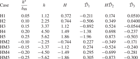
Case studies for different roughness shapes, where  $R=131820$,
 $d^{*}/\delta _{99}=8.0$,
 $d=0.495$ and
 $D=0.938$ for all cases.

The second-order amplitude equation yields
 \begin{equation} C_1= C_{10}+ b(X), \end{equation}
where
 \begin{gather} C_{10}={-}{\textrm{i}}{C_0}\left(K_5\int_{-\infty}^{X} AX\ \textrm{d}X-hK_0 K_2\int_{-\infty}^{X}f\kern0.05em X \ \textrm{d}X\right), \quad K_5=K_3-K_0 K_2, \end{gather}
 \begin{gather} b(X)=C_0 ({-}K_2-{\textrm{i}}K_4)X. \end{gather}
The term  $b(X)$ matches with the outer-region solution (A9), which is purely driven by the non-parallelism of the Blasius base flow. On the other hand,
 $C_{10}$ is associated with the interaction of the roughness-distorted mean flow with the non-parallelism of the perturbation profile. Indeed, the second-order scattering is only linked to
 $C_{10}$. Because the roughness impact on the oncoming modes in the upstream limit is negligible, we have put
 $C_{10}\rightarrow 0$ as
 $X\rightarrow -\infty$. However, the integral
 $\int _{-\infty }^{X} AX\ \textrm {d}X$ may not converge as
 $X\rightarrow \infty$, indicating a re-scattering effect induced by the roughness ‘wake’, which is the same as the T–S scattering in Wu & Dong (Reference Wu and Dong2016b). In the latter work, the divergent integral was interpreted as a Hardmard finite-part integral, and a transmission coefficient independent of the computational domain was obtained. In this paper, we are going to compare the asymptotic predictions with the numerical results, for which the amplitude growth of the perturbation in the downstream limit may be slightly different from that of the smooth-surface configuration, as will be shown in figure 15. Such a phenomenon can also be observed in the DNS results of Fong et al. (Reference Fong, Wang and Zhong2014, Reference Fong, Wang and Zhong2015b). Therefore, in the HLNS or DNS calculations, we choose the transmission coefficient from the perturbation amplitude at the outlet of the computational domain. This choice also agrees with the physical situation, for which laminar–turbulent transition or the nonlinear state may occur before the asymptotic state is reached. Therefore, in the asymptotic theory, we define
 \begin{equation} {\mathscr{T}}_1\equiv C_{10}(X_{HLNS})={-}{\textrm{i}} {\mathcal{B}} {\mathscr{T}}_0, \end{equation}
where  $X_{HLNS}\gg 1$ is the converted outlet boundary from the HLNS computational domain (as will be defined in (3.8)),
 \begin{equation} \left.\begin{gathered} {\mathcal{B}}=K_5{\mathcal{D}}_3-hK_0K_2{\mathcal{D}}_4,\\ {\mathcal{D}}_3=\int_{-\infty}^{X_{HLNS}} A(X)X\ \textrm{d}X,\quad {\mathcal{D}}_4=\int_{-\infty}^{X_{HLNS}} f(X)X\, \textrm{d}X. \end{gathered}\right\} \end{equation}
Note that if the roughness is symmetric along its centreline  $X=0$,
 ${\mathcal {D}}_4$ would be zero as long as
 $X_{HLNS} \geqslant d/2$, but
 ${\mathcal {D}}_3$ would not. Admittedly,
 ${\mathscr {T}}_1$ may vary if the computational domain of the HLNS calculation is changed. However, because
 ${\mathscr {T}}_1$ has only a second-order impact, the variation of the total transmission coefficient
 ${\mathscr {T}}$ would be rather mild. More importantly, this variation agrees with the numerical results obtained by the HLNS and DNS approaches, which can well reflect the physical situation.
Following Wu & Dong (Reference Wu and Dong2016b), the impact of the roughness on the oncoming Mack modes can be quantified by a transmission coefficient,
 \begin{equation} {\mathscr{T}}={\mathscr{T}}_0+O(\epsilon)+\varDelta_1{\mathscr{T}}_1+\cdots, \end{equation}
where the  $O(\epsilon )$ terms is caused by the second-order mean-flow distortion induced by the roughness, which is not taken into account in this paper. It is easy to see that the oncoming Mack mode is enhanced by the roughness if
 $|{\mathscr {T}}|>1$, but is suppressed if
 $|{\mathscr {T}}|<1$. It is estimated from (2.32) and (2.37) that
 \begin{gather} |{\mathscr{T}}|=\exp\left[ K_{0,i}({\mathcal{D}}_1+h{\mathcal{D}}_2)\right](1+\varDelta_1{\mathcal{B}}_i), \end{gather}
 \begin{gather}\arg({\mathscr{T}})={-}K_{0,r}({\mathcal{D}}_1+h{\mathcal{D}}_2)+\arg(1-{\textrm{i}} \varDelta_1{\mathcal{B}}), \end{gather}
where the subscripts  $r$ and
 $i$ denote the real and imaginary parts, respectively. For a relatively low roughness, for which
 $K_{0,i}({\mathcal {D}}_1+h{\mathcal {D}}_2)\ll 1$, the norm of the transmission coefficient (2.40) is estimated by
 \begin{equation} |{\mathscr{T}}|=1+ K_{0,i} {\mathcal{D}}_1+hK_{0,i} {\mathcal{D}}_2+\varDelta_1 {\mathcal{B}}_i+\cdots. \end{equation}
It is clearly seen from (2.42) that the local scattering effect is mainly attributed to three factors: (i)  $K_{0,i}{\mathcal {D}}_1$, the interaction between the mean-flow distortion and the oncoming Mack mode in the main layer; (ii)
 $hK_{0,i}{\mathcal {D}}_2$, the inhomogeneous forcing from the curved wall (Stokes layer); (iii)
 $\varDelta _1{\mathcal {B}}_i$, the interaction of the non-parallelism of the oncoming normal modes with the roughness-induced mean-flow distortion, which is merely the second-order effect. Whether the roughness plays a stabilising or destabilising role depends on their summed effects.
2.4. Improved asymptotic theory: taking into account the Stokes-layer impact
At a moderate Reynolds number, the linear instability mode (2.10) for a smooth-surface configuration is described by the compressible O–S equation system as in Mack (Reference Mack1987), Malik (Reference Malik1990) and Wu & Dong (Reference Wu and Dong2016a). In the original asymptotic theory, because the viscosity in the main layer is negligible to the orders of our concern, the instability is described by the Rayleigh equation (2.14) with (2.18a,b), which allows a slip velocity at the wall, i.e.  $\hat {u}(0)\ne 0$. In order to satisfy the no-slip condition, a viscous Stokes layer in the
 $O(\epsilon ^{2})$ vicinity of the wall, as shown in figure 2, has to be introduced; a detailed analysis can be found in Dong et al. (Reference Dong, Liu and Wu2020). The Stokes layer generates an
 $O(\epsilon ^{2})$ correction to the main layer, leading to an improved boundary condition (Dong et al. Reference Dong, Liu and Wu2020),
 \begin{equation} \hat{v}(0)={-}\epsilon^{2}{\mathcal{C}}\hat p(0),\quad{\mathcal{C}}=C_w^{1/2}\left[\frac{\tilde\alpha^{2}T_w}{(-{\textrm{i}}\omega)^{3/2}}+\frac{{\textrm{i}}(\gamma-1)\omega M^{2}}{(-{\textrm{i}}\omega {Pr})^{1/2}}\right], \end{equation}
where  $-{\textrm {i}}\equiv {\textrm {e}}^{3{\rm \pi} {\textrm {i}}/2}$ and
 $C_w=\mu (T_w)T_w$. Therefore, (2.14) with (2.43a,b) and (2.18b) form an improved Rayleigh system. By taking the
 $O(\epsilon ^{2})$ correction into account, the improved Rayleigh system can predict the dispersion relation of the Mack mode more accurately at a moderate Reynolds number; see Dong et al. (Reference Dong, Liu and Wu2020).
For convenience, we can re-express the improved Rayleigh system as
 \begin{align} &\bar{\mathcal{L}}_R\hat{\boldsymbol \phi}\equiv(\partial_y-\bar{{\boldsymbol{\mathsf{H}}}}_0)\hat{\boldsymbol \phi}=0, \end{align}
 \begin{align} &\bar{\mathcal{L}}_R\hat{\boldsymbol \phi}_1={-}{\textrm{i}}\frac{\partial \bar{{\boldsymbol{\mathsf{H}}}}_0}{\partial \alpha}C'_0(X)\hat{\boldsymbol \phi}+\bar{{\boldsymbol{\mathsf{H}}}}_1A(X)C_0(X)\hat{\boldsymbol \phi}+hf(X)C_0(X)\delta(y){\boldsymbol{\mathsf{D}}}, \end{align}
 \begin{align} &\bar{\mathcal{L}}_R\hat{\boldsymbol \phi}_2=\displaystyle-{\textrm{i}}\frac{\partial {{\boldsymbol{\mathsf{H}}}}_0}{\partial \alpha}[C'_1\hat{\boldsymbol \phi}+(C_0'X+C_0)\hat{\boldsymbol \phi}_{\bar{x}}] +{{\boldsymbol{\mathsf{H}}}}_1A(C_1\hat{\boldsymbol \phi}+C_0X\hat{\boldsymbol \phi}_{\bar{x}})+{{\boldsymbol{\mathsf{H}}}}_2C_0\hat{\boldsymbol \phi}\nonumber\\ &\qquad +hfC_1\delta(y){\boldsymbol{\mathsf{D}}}, \end{align}
 \begin{align} &\hat{\psi}_{(1)}(0)=\{\tilde{\psi}_1\}_{(1)}(X,0)=\{\tilde\psi_2\}_{(1)}(X,0)=0, \end{align}
 \begin{align} &(\hat{\psi}_{(2)}(y),\{\tilde{\psi}_1\}_{(2)}(X,y),\{\tilde\psi_2\}_{(2)}(X,y))\rightarrow 0\quad\mbox{as }y\rightarrow\infty, \end{align}
where  ${\boldsymbol \phi} =(\psi _{(1)},\psi _{(2)})^\textrm {T}\equiv (v+\epsilon ^{2}{\mathcal {C}} p,p)^\textrm {T}$, and
 \begin{equation} \bar{{\boldsymbol{\mathsf{H}}}}_{l}=\left(\begin{array}{cc} \{{{{\mathsf{H}}}}_{l}\}_{11}+\epsilon^{2}{\mathcal{C}}\{{{{\mathsf{H}}}}_{l}\}_{21} & \{{{{\mathsf{H}}}}_{l}\}_{12}-\epsilon^{2}{\mathcal{C}}\left(\{{{{\mathsf{H}}}}_{l}\}_{11}+\epsilon^{2}{\mathcal{C}}\{{{{\mathsf{H}}}}_{l}\}_{21}\right) \\ \{{{{\mathsf{H}}}}_{l}\}_{21} & -\epsilon^{2} {\mathcal{C}}\{{{{\mathsf{H}}}}_{l}\}_{21} \end{array}\right)\quad (l=1,2). \end{equation}
The adjoint system is thus given by
 \begin{gather} (\partial_y+\bar{{\boldsymbol{\mathsf{H}}}}_0^{T})\hat{\boldsymbol \phi}^{{\dagger}ger}=0,\end{gather}
 \begin{gather} \hat{\psi}^{{\dagger}ger}_{(2)}(0)=0,\quad\hat\psi^{{\dagger}ger}_{(1)}(y)\rightarrow 0\quad\mbox{as }y\rightarrow\infty. \end{gather}
The transmission coefficient can also be calculated by (2.40) or (2.42), but with  $\hat{\boldsymbol\phi}$,
 $\hat{\boldsymbol\phi}^{{\dagger} }$ and
 ${{\boldsymbol{\mathsf{H}}}}_{0,1}$ in (2.28a,b) being replaced by
 $\hat{\boldsymbol \phi}$,
 $\hat{\boldsymbol \phi}^{{\dagger} }$ and
 $\bar {{\boldsymbol{\mathsf{H}}}}_{0,1}$, respectively.
3. DNS and HLNS approaches
3.1. DNS approach
Alternatively, one can re-express the full N–S equations (2.2) in terms of the conservative form (Qin & Dong Reference Qin and Dong2016) and solve the nonlinear equation system directly by numerical schemes, which is referred to as DNS. The DNS code in this paper is the same as that used in Zhao et al. (Reference Zhao, Dong and Yang2019) and Zhao & Dong (Reference Zhao and Dong2020).
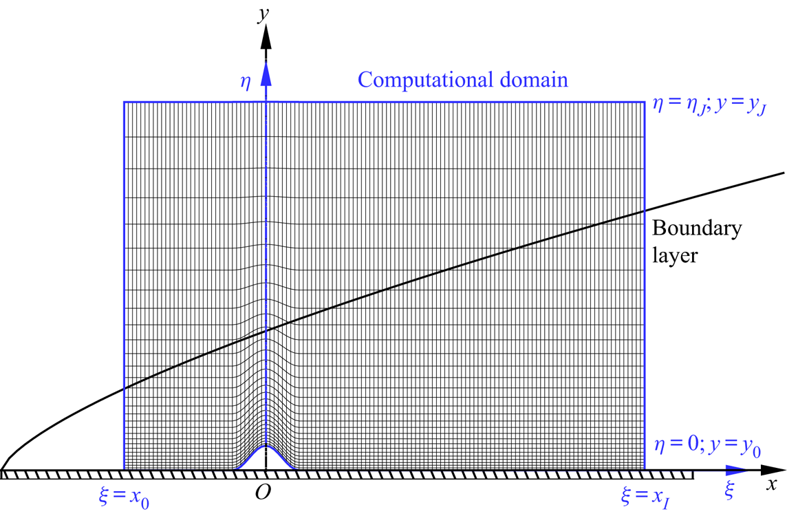
The calculations include two steps. First, one needs to calculate the steady solution of the roughness-distorted mean flow,  $\bar{\boldsymbol\varphi}$ in (2.4). Since the roughness is assumed to be two-dimensional, we simply choose a 2-D body-fitted coordinate system
 $(\xi ,\eta )$ with a 2-D computational domain
 $x_0 \leqslant \xi \leqslant x_I$ and
 $0 \leqslant \eta \leqslant \eta _J$, as shown in figure 3. Upstream and downstream of the roughness, the body-fitted coordinate system is the same as the original Cartesian system, while at the roughness the transverse coordinate
 $\eta$ is curved such that the wall surface
 $y=y_0$ is converted to
 $\eta =0$. A total of
 $I+1$ uniform grid points are used in the streamwise direction, while
 $J+1$ non-uniform grid points that are clustered in the near-wall region are used in the wall-normal direction. Each grid point is labelled by
 $(i,j)$ with
 $i\in [0,I]$ and
 $j\in [0,J]$. The convective and viscous terms are discretised by the fifth-order partial and fourth-order central finite difference schemes, respectively, and the third-order Runge–Kutta method is used for time advancing. At the inlet of the computational domain,
 $\xi =x_0$, the Blasius solution is introduced because the impact of the roughness is somewhat local. The no-slip, non-penetration and isothermal conditions are imposed at the wall,
 $\eta =0$. A buffer region is introduced at the outlet
 $\xi =x_I$, and the outflow condition is used at the upper boundary
 $\eta =\eta _J$. The calculation is carried out until the solution converges to be time independent.
Sketch of the mesh system and computational domain for DNS and HLNS calculations.

Second, we calculate the unsteady perturbation field  $\tilde {\varphi }$ in the selected computational domain. If the perturbation is three-dimensional, we need to introduce a spanwise coordinate
 $z$ and extend the mean flow such that it is uniform in the
 $z$-direction. The numerical approach is exactly the same as that of the first step except for the inflow condition, which is changed to the superposition of a steady mean flow and a harmonic Mack mode with an infinitesimal amplitude,
 \begin{equation} {\boldsymbol{\varphi}}(x_0,y,z,t)=\bar{\boldsymbol\varphi}(x_0,y)+\tilde{\boldsymbol\varphi}(x_0,y,z,t). \end{equation}
The latter is the eigensolution of the compressible O–S equations based on the mean profile at  $\xi =x_0$,
 \begin{equation} \tilde{\boldsymbol\varphi}(x,y,z,t)={\mathcal{E}}\hat{\boldsymbol\varphi}(y) \exp\left({{\textrm{i}}\left(\int_{x_0}^{x} \alpha \,{\textrm{d}\kern0.06em x}+\beta z-\omega t\right)}\right)+\textrm{c.c.}, \end{equation}
and the amplitude  $\mathcal {E}$ is taken to be
 $10^{-10}$.
In this paper, we perform 2-D calculations and choose  $x_0=-50$,
 $x_I=245$,
 $y_J=80$,
 $I=2000$ and
 $J=300$. The buffer region is introduced in the interval
 $x\in [245,530]$, in which
 $300$ grid points are assigned. After obtaining the perturbation field, we calculate the transmission coefficient using
 \begin{equation} {\mathscr{T}}=\frac{\displaystyle\max_{t>t_0}[\tilde{p}(x_I,0,t_0)]_{roughness}}{\displaystyle\max_{t>t_0}[\tilde{p}(x_I,0,t_0)]_{smooth-surface}}, \end{equation}
where  $t_0$ is a time instant after which the perturbation field is statistically steady.
3.2. HLNS approach
If the mean flow has been obtained by the first step of § 3.1, we can calculate the perturbation evolution (the second step) in a more efficient manner. As illustrated in Zhao et al. (Reference Zhao, Dong and Yang2019) and Zhao & Dong (Reference Zhao and Dong2020), an infinitesimal perturbation can be expressed as
 \begin{equation} \tilde{\boldsymbol\varphi}={\mathcal{E}}\breve{\boldsymbol\varphi}(\xi,\eta)\exp({{\textrm{i}}\alpha_0\xi})\exp({{\textrm{i}} (\beta z-\omega t)})+\textrm{c.c.}, \end{equation}
where  $\alpha _0$ is a reference complex wavenumber introduced for numerical convenience. Here,
 $\alpha _0$ is simply selected as the eigenvalue solution of the compressible O–S equations at the inlet
 $\xi =x_0$. Substituting (3.4) into the N–S equation system and neglecting the
 $O({\mathcal {E}}^{2})$ terms, we obtain a linear system,
 \begin{equation} (\tilde{\boldsymbol{\mathsf{D}}}+\tilde{\boldsymbol{\mathsf{A}}}\partial_\xi+\tilde{\boldsymbol{\mathsf{B}}}\partial_\eta+ \tilde{\boldsymbol{\mathsf{V}}}_{\xi\xi}\partial_{\xi\xi}+\tilde{\boldsymbol{\mathsf{V}}}_{\eta\eta}\partial_{\eta\eta}+ \tilde{\boldsymbol{\mathsf{V}}}_{\xi\eta}\partial_{\xi\eta})\breve{\boldsymbol\varphi}(\xi,\eta)=0, \end{equation}
where the coefficient matrices  $\tilde {\boldsymbol{\mathsf{D}}}$,
 $\tilde{\boldsymbol{\mathsf{A}}}$,
 $\tilde{\boldsymbol{\mathsf{B}}}$,
 $\tilde{\boldsymbol{\mathsf{V}}}_{\xi \xi }$,
 $\tilde{\boldsymbol{\mathsf{V}}}_{\eta \eta }$ and
 $\tilde{\boldsymbol{\mathsf{V}}}_{\xi \eta }$ can be found in the appendix of Zhao et al. (Reference Zhao, Dong and Yang2019). Under a proper discretisation, the linear system (3.5) is reduced to a system of algebraic equations,
 \begin{equation} \tilde{\boldsymbol{\mathsf{M}}}\tilde{\boldsymbol q}=\tilde{\boldsymbol r}, \end{equation}
where the coefficient matrices  $\tilde{\boldsymbol{\mathsf{M}}}$, the unknown vector
 $\tilde {\boldsymbol {q}}$ and the inhomogeneous forcing
 $\tilde {\boldsymbol {r}}$ were illustrated in Zhao et al. (Reference Zhao, Dong and Yang2019).
Usually a sizable roughness element would induce a shock wave radiating to the far field. It was reported by Zhao et al. (Reference Zhao, Dong and Yang2019) that, as long as the shock is not too strong, the evolution of the perturbation calculated by the HLNS approach is rather precise, as confirmed by DNS, but the computational cost of the former is tiny.
In the HLNS calculation, the computational domain is the same as that in § 3.1, and  $1001\times 301$ grid points are employed, which is only a half of those used in DNS. Careful resolution studies have been carried out. The transmission coefficient now is defined as
 \begin{equation} {\mathscr{T}}=\frac{|\breve{p}(x_I,0)|_{roughness}}{|\breve{p}(x_I,0)|_{smooth-surface}}. \end{equation}
Note that  $X_{HLNS}$ defined in (2.37) is related to
 $x_I$ via
 \begin{equation} X_{HLNS}=\epsilon x_I. \end{equation}
4. Numerical results
4.1. Oncoming conditions and the base flow
Following Fong et al. (Reference Fong, Wang and Zhong2014, Reference Fong, Wang and Zhong2015b) and Zhao et al. (Reference Zhao, Dong and Yang2019), we choose  $M=5.92$,
 $T_\infty =48.69$ K and
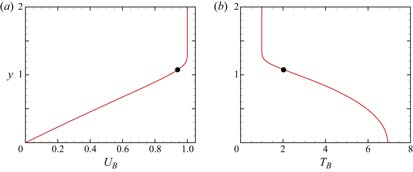
 $T_w=6.95$. Figure 4 shows the wall-normal profiles of the streamwise velocity
 $U_B$ and temperature
 $T_B$ of the compressible Blasius solution, in which the location of the generalised inflectional point (GIP)
 $y_c$ is marked. Table 1 also lists the factor
 $\varDelta$, the nominal boundary-layer thickness
 $\delta _{99}$, the location of the GIP
 $y_c$ and the streamwise velocity at the GIP
 $U_c$. Two Reynolds numbers,
 $R=131\,820$ and 26 364, are chosen for representative demonstration. The former is used to confirm the accuracy of the asymptotic theories, and the latter is used to compare with the numerical results of Zhao et al. (Reference Zhao, Dong and Yang2019).
The streamwise velocity (a) and temperature (b) of the compressible Blasius solution. The dots indicate the location of the GIP.

Key parameters characterising the base flow.

4.2. Instability
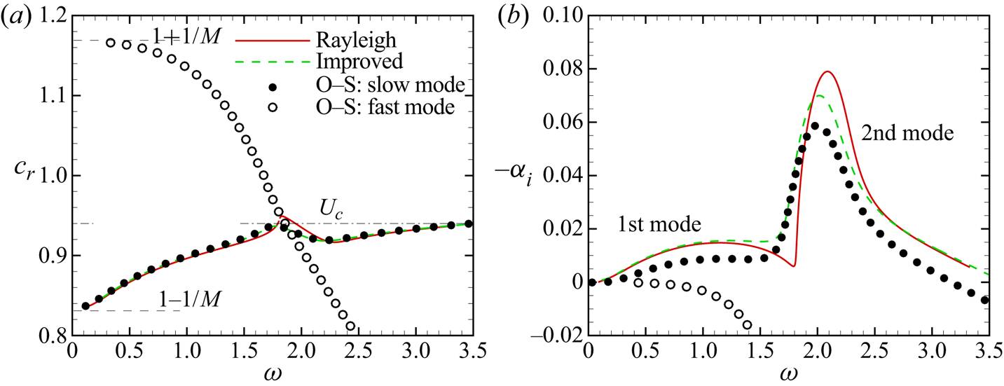
Figure 5 plots the phase speed and growth rate of the 2-D Mack modes based on the Blasius profile at  $x=0$. Note that our theory also applies for 3-D instability modes. Solving the compressible O–S equations for
 $R=26\,364$, we obtain two branches of instability modes, which are shown as the filled and open circles. As
 $\omega \rightarrow 0$, the phase speeds of the two branches, shown in figure 5(a), approach
 $1-1/M$ and
 $1+1/M$, corresponding to the phase speeds of the slow and fast acoustic waves in the external stream with zero incident angle, respectively. Therefore, the two branches of instability modes are referred to as modes
 $S$ and
 $F$, respectively. As figure 5(b) indicates, only the mode
 $S$ can be unstable in certain frequency bands, and its growth rate exhibits two peaks located at
 $\omega \approx 1.2$ and 2.0, respectively. Following the definition of Mack (Reference Mack1987), the instability modes in the lower and higher frequency bands are referred to as the first and second Mack modes, respectively. They intersect when the growth rate reaches a local minimum. The second mode is more unstable overall. The phase speeds of modes
 $F$ and
 $S$ intersect at
 $\omega \approx 1.9$, which is referred to as the synchronisation point (frequency), despite the fact that their growth rates
 $-\alpha _i$ differ by an amount that is numerically small (in comparison with
 $\alpha _r$); see Fedorov (Reference Fedorov2011). For both the first and second modes, as
 $\omega$ approaches the upper-branch neutral frequency or the synchronisation frequency of modes
 $F$ and
 $S$, the phase speed
 $c_r$ approaches
 $U_c$, the streamwise velocity of the Blasius solution at the GIP.
Dependence of the phase speed  $c_r$ (a) and the growth rate
 $-\alpha _i$ (b) of 2-D Mack modes on the frequency
 $\omega$. For the O–S solution and improved Rayleigh solution, we select
 $R=26\,364$.

The solutions of the Rayleigh equations (2.14), shown as the red solid lines, exhibit a similar trend as those of the compressible O–S equations, but a quantitative discrepancy is observed. The growth rates of both the first and second modes of the Rayleigh solutions are overall higher than those of the O–S solutions, implying that the viscosity plays a stabilising role. The improved Rayleigh equations (2.44), for which the impact of the Stokes layer is included, provide better predictions of both  $c_r$ and
 $\alpha _i$, as the green dashed lines indicate.
4.3. Mean-flow distortion
The mean-flow distortion induced by the wall roughness (2.5) is obtained by solving numerically the triple-deck system as shown in appendix B. The accuracy of the triple-deck calculations, obtained by comparing with the DNS results in subsonic and transonic boundary layers, has been confirmed by Mengaldo et al. (Reference Mengaldo, Kravtsova, Ruban and Sherwin2015), and it was found that, for a roughness element with a height of  $0.15\delta _{99}$, the error is less than
 $3\,\%$. In this subsection, we carry out comparisons in supersonic regime. Note that in the triple-deck system the Mach number, Reynolds number and wall temperature are scaled out, and so the control parameters are only
 $H$ and
 $D$, denoting the re-scaled height and width of the roughness, as introduced in (B3a,b). Table 2 lists a number of representative cases for
 $R=131\,820$, in which five humps and four indentations with the same width but different heights are included. Three quantities associated with the efficiency of the scattering effect are also shown,
 \begin{equation} \bar{\mathcal{D}}_1=\int_{-\infty}^{\infty} \tilde{A}\ \textrm{d}\tilde{X},\quad \bar{\mathcal{D}}_2= H\int_{-\infty}^{\infty} \tilde{f}\ \textrm{d}\tilde{X}, \quad\bar{\mathcal{D}}_3=\int_{-\infty}^{\tilde{X}_{HLNS}} \tilde{X}\tilde{A}\ \textrm{d}\tilde{X}, \end{equation}
where  $\tilde {X}_{HLNS}={\mathcal {R}}_XX_{HLNS}$. Note that, even for case H1, the case for the smallest hump height, the mean-flow distortion already exhibits a weak nonlinear effect since
 $\bar {\mathcal {D}}_1+H\bar {\mathcal {D}}_2$ is slightly negative, which is in contrast to the linear case, as illustrated in appendix B.2.
4.3.1. Comparison between the triple-deck and DNS results
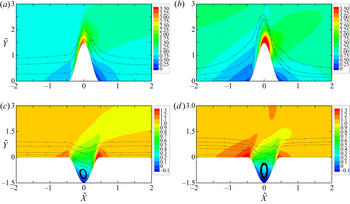
Figure 6 compares the mean shear and the streamlines in the near-wall region obtained by the triple-deck theory with those obtained by DNS. The coordinate system and velocity field of the DNS results are converted to the triple-deck scalings through the relations (B1a,b) and (B5a–c). For a hump case with  $h^{*}/\delta _{99}=0.20$, shown in figure 6(a,b), both the triple-deck and DNS results exhibit a high-shear region on the top of the hump and two low-shear regions at its two sides. For an indentation case with
 $h^{*}/\delta _{99}$=-0.20, as figure 6(c,d) indicates, a low-shear region and two high-shear regions appear in the bottom and at the two sides, respectively, and a circulation appears inside the indentation. Quantitative differences between the two calculations exist due to the finite-
 $R$ effect.
Contours of the mean shear  $\tilde {U}_{\tilde {Y}}$ and the streamlines in the close neighbourhood of the roughness for cases H4 (a,b) and HM4 (c,d), where the left and right columns are for results obtained by triple-deck calculation and DNS, respectively.

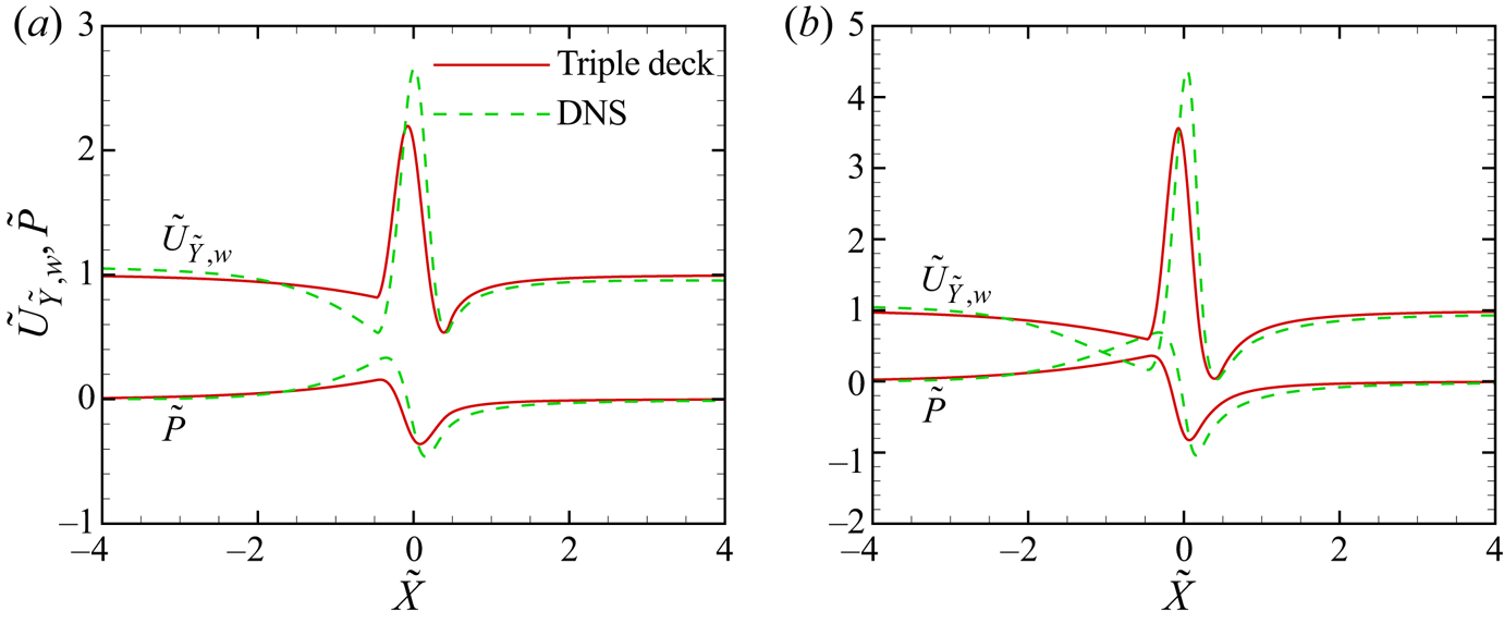
Figure 7 compares the wall shear and the wall pressure between the triple-deck and DNS results. For both the two hump heights,  $h^{*}/\delta _{99}=0.10$ and 0.20, the two families of curves agree in quality. The mean-flow distortion obtained by DNS is slightly larger in the region
 $-1 \leqslant \tilde {X} \leqslant 0.4$. The relative error stays at the same level as
 $H$ increases. Note that this comparison is for a relatively large Reynolds number, and as
 $R$ decreases, the agreement becomes worse due to the impact of the neglected
 $O(\epsilon ^{2})$ terms.
Comparison of the wall shear  $\tilde {U}_{\tilde {Y},w}$ and the wall pressure
 $\tilde {P}$ between triple-deck and DNS results. (a,b) Are for cases H2 and H4, respectively.

The triple-deck theory can also provide a composite solution for the whole boundary-layer profile,
 \begin{equation} \bar{U}_{com}=\bar{U} +\epsilon{\mathcal{R}}_U^{{-}1}\tilde{U}-U_B'(0)\left(y+\epsilon A(X)\right), \end{equation}
where  $\bar {U}$ is the mean flow in the main layer defined in (2.7), and
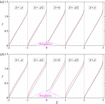
 $\tilde {U}$ is the lower-deck solution introduced in appendix B. Figure 8 compares the composite solutions near the roughness with the DNS results for cases H2 and H4. For a relatively low hump, the mean-flow distortion is quite weak, but we can still see that the general trends of the mean-flow distortions obtained by the two approaches agree overall. Slight discrepancies are observed at the two ends of the roughness, i.e.
 $X\approx \pm d/2$. The discrepancies increase with the roughness height. Interestingly, in the near-wall region, the agreement between the two calculations is much better, which confirms the observations from figure 7.
Profiles of the mean streamwise velocity  $\bar {U}$ at five representative stations near the roughness for cases H2 (a) and H4 (b), where the red solid and blue dashed lines are for the DNS results and triple-deck composite solutions (4.2), respectively. The profiles are shifted horizontally for plotting convenience. The thin solid lines denote the Blasius solution for the smooth-surface case.

4.3.2. Mean-flow distortion for different cases
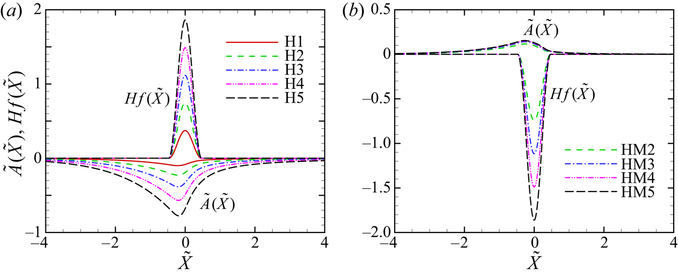
Figure 9 compares the displacement function  $\tilde {A}(\tilde {X})$ and the wall function
 $H\tilde {f}(\tilde {X})$ for different hump heights or indentation depths. For each hump case, shown in figure 9(a), the displacement function
 $\tilde {A}$ is negative in the vicinity of the hump and approaches zero in both the upstream and downstream limits. By contrast,
 $\tilde {A}$ for each indentation, shown in figure 9(b), is positive. Both panels indicate that
 $\tilde {A}$ distributes in a wider range than the wall shape
 $H\tilde {f}$ does. The mean-flow distortion, measured by the absolute value of
 $\tilde {A}$, is greater for a higher hump, but varies only slightly as the indentation depth increases.
The streamwise distributions of the displacement function  $\tilde {A}$ and the shape of the roughness
 $Hf(\tilde {X})$. (a) Hump cases H1 to H5; (b) indentation cases HM2 to HM5.

As revealed by (2.42), the scattering effect is attributed to three factors associated with the mean-flow distortion, i.e.
 \begin{equation} {\mathcal{D}}_1={\mathcal{R}}_X^{{-}1}{\mathcal{R}}_Y^{{-}1}\bar{\mathcal{D}}_1,\quad h{\mathcal{D}}_2={\mathcal{R}}_X^{{-}1}{\mathcal{R}}_Y^{{-}1}H\bar{\mathcal{D}}_2,\quad {\mathcal{D}}_3={\mathcal{R}}_X^{{-}2}{\mathcal{R}}_Y^{{-}1}\bar{\mathcal{D}}_3, \end{equation}
and the values of  $\bar {\mathcal {D}}_1$,
 $H\bar {\mathcal {D}}_2$ and
 $\bar {\mathcal {D}}_3$ for the chosen cases are also listed in table 2. Note that the quantity
 $\int _{-\infty }^{\infty } \tilde {X}\tilde {f}\ \textrm {d}\tilde {X}$ is always zero in this paper because the shapes of the humps and indentations are all symmetric about
 $\tilde {X}=0$. For a linear hump or indentation, for which
 $|H|\ll 1$,
 $\bar {\mathcal {D}}_1$ is equal to
 $H{\mathcal {D}}_2$ exactly, as (B18) indicates, which implies that a linear roughness does not have any impact on the oncoming Mack modes to leading-order accuracy. For nonlinear roughness cases,
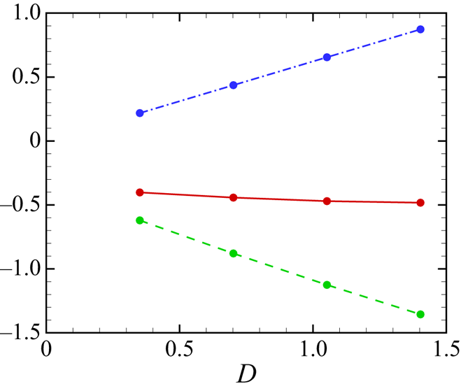
 $\bar {\mathcal {D}}_1$ decreases remarkably with the hump height for cases H1 to H5, but increases mildly with the indentation depths for cases HM2 to HM5. Because the hump heights of cases H2 to H5 are opposite to the indentation depths of cases HM2 to HM5, the values of
 $H\bar {\mathcal {D}}_2$ between each counterpart (H
 $l$ and HM
 $l$ with
 $l=2$ to 5) are exactly opposite;
 $\bar {\mathcal {D}}_3$ is one order of magnitude smaller than
 $\bar {\mathcal {D}}_1$ for small hump cases, but increases to the same order of magnitude as the latter for moderate hump and all indentation cases.
4.4. Scattering calculations
4.4.1. Efficiency functions
From (2.28a,b) and (2.35a,b), we calculate the efficiency functions  $K_0$ and
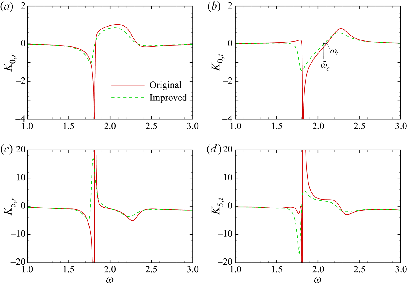
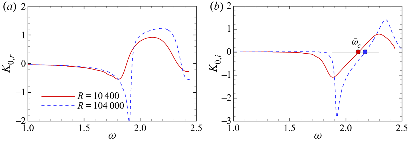
 $K_5$ using the original asymptotic theory in § 2.3 and the improved asymptotic theory in § 2.4, as shown in Figure 10. Note that the efficiency functions obtained by the original asymptotic theory are independent of
 $R$, but those by the improved theory are not. For the latter calculations, we choose
 $R=131\,820$. All the panels show that the efficiency functions vary remarkably in the frequency band
 $1.5<\omega <2.5$, corresponding to most of the second mode and a small portion of the first mode. It is easy to see from (2.40) and (2.41) that a relatively strong scattering effect may appear in this frequency band. For the original asymptotic theory, as
 $\omega$ increases from 1.5,
 $K_{0,r}$ falls dramatically and there is a valley at around
 $\omega =1.8$; it then rises sharply to positive and exhibits a wide bump shape before falling back to zero. As shown in panel (b),
 $K_{0,i}$ increases with
 $\omega$ slightly from
 $\omega =1.5$, but falls drastically at
 $\omega \approx 1.8$; after reaching its valley at approximately
 $\omega =1.815$,
 $K_{0,i}$ increases with
 $\omega$ again and peaks at
 $\omega \approx 2.28$; it falls back towards zero as
 $\omega$ further increases. The frequency
 $\omega _c=2.10$ for which
 $K_{0,i}=0$ is marked in panel (b), which, according to (2.40) or (2.42), represents the critical frequency distinguishing the stabilising and destabilising effects of the roughness to leading-order accuracy. This frequency is quite close to the synchronisation frequency, as shown in figure 5, which agrees with the DNS results in Fong et al. (Reference Fong, Wang and Zhong2014, Reference Fong, Wang and Zhong2015b).
Dependence of the efficiency functions  $K_0$ (a,b) and
 $K_5$ (c,d) on frequency
 $\omega$. The thin horizontal line in (b) represents the zero line, and
 $\omega _c=2.10$ and
 $\bar \omega _c=2.07$ are the frequencies for which
 $K_{0,i}$ crosses the zero line.

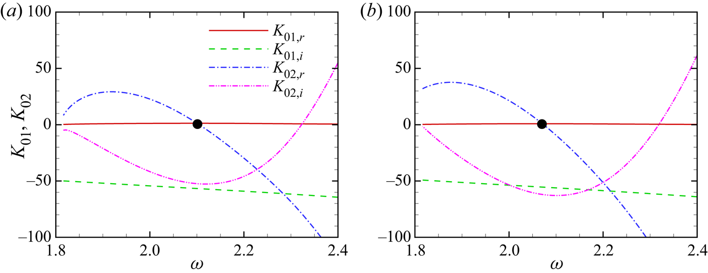
In order to probe the intrinsic mechanism, we plot separately the numerator  $K_{01}=\langle \hat{\boldsymbol\phi},{{\boldsymbol{\mathsf{H}}}}_1\hat{\boldsymbol\phi}\rangle$ and the denominator
 $K_{02}=\langle \hat{\boldsymbol\phi},(\partial {{\boldsymbol{\mathsf{H}}}}_0/\partial \alpha )\hat{\boldsymbol\phi}\rangle$, as shown in figure 11(a). The numerator
 $K_{01}$ is almost pure imaginary, which can be predicted analytically as follows. As is proven in appendix C, the numerator
 $K_{01}$ is equal to
 $\langle \hat{\boldsymbol\phi}^{{\dagger} },\delta (y)\boldsymbol {D}\rangle$. The latter can be expressed as
 \begin{equation} -\hat{\phi}^{{\dagger}ger}_{(1)}(0)\hat{v}_y(0)={\textrm{i}}\left({-}M^{2}\omega+\frac{(\alpha_r^{2}-\alpha_i^{2}+\beta^{2})T_w}{ \omega}\right) -\frac{2\alpha_r\alpha_iT_w}{\omega}. \end{equation}
Since  $|\alpha _i|\ll \alpha _r$, the real part of the right-hand side of (4.4) is much smaller than its imaginary part. Therefore,
 $K_{0,i}$ crosses zero when
 $K_{02,r}\approx 0$, which appears at
 $\omega \approx 2.1$, as shown by the filled circle in figure 11(a). Figure 12 plots the wall-normal profiles of the real part of the integrand of
 $K_{02}$,
 $[(\hat{\boldsymbol\phi}^{{\dagger} })^\textrm {T}(\partial {\boldsymbol{\mathsf{H}}}_0/\partial \alpha )\hat{\boldsymbol\phi}]_r$, for three representative frequencies. These profiles are all concentrated around the edge of the boundary layer, and their positive and negative parts contribute oppositely to the integral
 $K_{02}$. For the critical frequency,
 $\omega \approx 2.1$, these opposite contributions cancel out, leading to
 $K_{02,r}\approx 0$. For higher and lower frequencies, the integrals become negative and positive, respectively, agreeing with figure 11(a).
Variation of the numerator and denominator of  $K_0\equiv K_{01}/K_{02}$ on
 $\omega$ in the second-mode frequency band obtained by the original (a) and improved (b) asymptotic theories.

Wall-normal profiles of the real part of the integrand of  $K_{02}$ for three representative frequencies.

For the improved asymptotic theory, as shown by the green dashed lines in figures 10(a) and 10(b), the overall trend is the same as that for the original asymptotic theory, but the curves vary more gently, especially in the region around  $\omega\approx 1.8$ and shift slightly towards the lower-frequency direction. A direct consequence is that the critical frequency
 $\omega _c$ is shifted to
 $\bar {\omega }_c=2.07$. Additionally, the denominator
 $K_{02}$ predicted by the original asymptotic theory, shown in figure 11(a), approaches zero as
 $\omega$ approaches 1.8, the intersection frequency of the first and second modes, indicating that the efficiency function
 $K_0$ obtained by the original theory tends to blow up at the frequency. However, for the improved theory, both
 $K_0$ and
 $K_{02}$ tend to be finite at
 $\omega \approx 1.8$, which is of course more reasonable.
The second-order scattering effect is linked to  $K_5$ as shown in figures 10(c) and 10(d). Both the real and imaginary parts of
 $K_5$ vary drastically in a narrow band
 $1.7<\omega <1.85$, which corresponds to the local peak frequency of the phase speed in figure 5. This is due to the small denominators of
 $K_2$ and
 $K_3$,
 ${\langle \hat{\boldsymbol\phi}^{{\dagger} },({\partial {{\boldsymbol{\mathsf{H}}}}_0}/{\partial \alpha })\hat{\boldsymbol\phi}\rangle }$, near
 $\omega =1.8$. Note that, in this narrow frequency band, the second-order efficiency function is almost one order of magnitude greater than the first-order efficiency function, indicating a potentially strong scattering effect contributing from the second order.
4.4.2. Comparison with the HLNS results for a relatively large Reynolds number
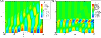
In order to verify the accuracy of the asymptotic theories, we perform DNS and HLNS to calculate the evolution of the Mack modes. Here, we choose case H4 and  $R=131\,820$. Figure 13 shows the contours of the instantaneous perturbation pressure and temperature for
 $\omega =1.78$ obtained by DNS. The value of
 $\tilde {p}$ peaks at the wall, while
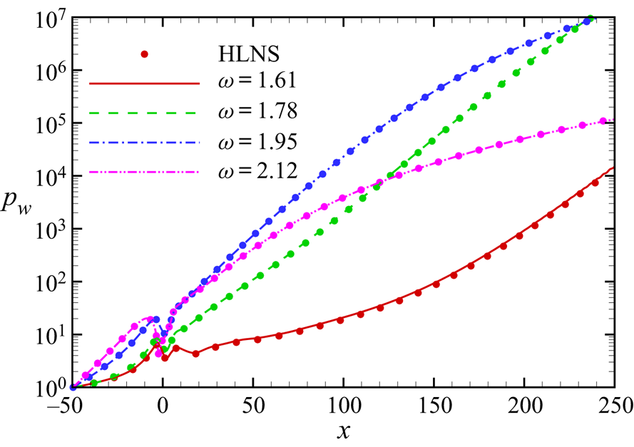
 $\tilde {T}$ peaks at the edge of the boundary layer. The perturbation profiles undergo rapid distortions in the vicinity of the hump and a Mach wave is radiated to the far field, as the pressure perturbation in panel (a) indicates. Figure 14 further plots the amplitude evolution of the wall pressure
 $p_w$ normalised by the value at the inlet boundary for four representative frequencies. For DNS calculations, the normalised wall pressure amplitude
 $p_w$ is defined as
 \begin{equation} p_w(x)=\frac{\displaystyle\max_{t>t_0}|\tilde{p}(x,\eta=0,t)|}{\displaystyle\max_{t>t_0}|\tilde{p}(x_0,\eta=0,t)|}, \end{equation}
where  $t_0$ has been defined in (3.3), and for HLNS calculations,
 \begin{equation} p_w(x)=|\breve{p}(x,\eta=0)\,{\textrm{e}}^{{\textrm{i}}\alpha_0 x}|. \end{equation}
Note that  $x$ is the same as
 $\xi$. The amplitude curves grow exponentially, but each curve exhibits a kink at the roughness. The HLNS calculations agree perfectly with the DNS results.
Contours of the instantaneous perturbation pressure (a) and temperature (b) obtained by DNS for case H4, where  $\omega =1.78$ and
 $R=131\,820$.

Amplitude evolution of the normalised perturbation pressure at the wall obtained by the DNS (continuous curves) and HLNS (circles) approaches for case H4, where  $R=131\,820$.

In order to quantify the scattering effect, we further normalise the perturbation amplitude by that of the smooth-surface configuration,
 \begin{equation} {\mathcal{A}}(x)=\frac{p_w|_{roughness}}{p_w|_{smooth-surface}}, \end{equation}
which is comparable with the amplitude evolution  $C$ defined in (2.12). Figure 15 shows the evolution of
 $\mathcal {A}$ for two representative frequencies for case H4. For
 $\omega =1.86$, the roughness plays a destabilising role. The normalised amplitude at the outlet boundary reflects the transmission coefficient, which is approximately 3.2 from DNS and HLNS calculations, although the amplitude curves decrease slightly in the downstream region. The latter is due to the re-scattering effect of the roughness ‘wake’, as discussed in § 2.3.3. The asymptotic prediction
 $C$ obtained by the improved theory agrees well with the numerical results downstream of the roughness, and the mild decrease of the normalised amplitude
 $\mathcal {A}$ with
 $\omega$ is clearly reproduced by the asymptotic theory. The leading-order prediction
 $C_0$ yields a small amount of error, which increases with
 $x$. In the close neighbourhood of the roughness, the numerical results exhibit a kink, which is over-predicted by the asymptotic theory appreciably. The discrepancy is due to the finite-
 $R$ effect. For a higher frequency,
 $\omega =2.20$, the roughness plays a stabilising role, but the asymptotic theory under-predicts this effect quantitatively. The transmission coefficient obtained by HLNS is approximately 0.35, but that predicted by the asymptotic theory is approximately 0.54. For the asymptotic theory, the second-order impact is rather weak because
 $K_5$ is quite small at this frequency. The kink predicted by the asymptotic theory near the roughness is not obvious in the numerical results. In summary, the asymptotic theory can predict the overall destabilising or stabilising effect of the roughness, although there exists an amount of quantitative error.
Amplitude evolution of the perturbations with  $\omega =1.86$ (a) and 2.20 (b) for case H4 obtained by HLNS, DNS and the improved asymptotic theory, where
 $C_0$ is the leading-order prediction.

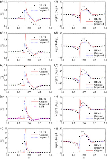
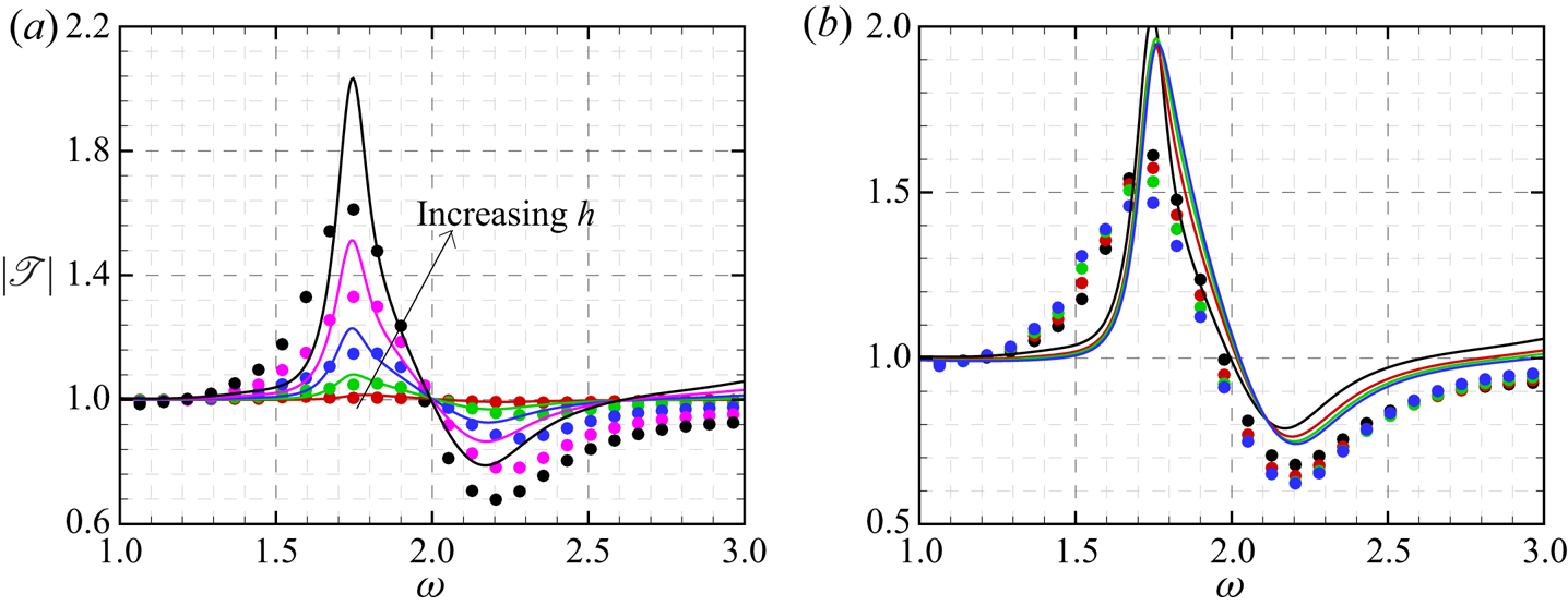
For each roughness height listed in table 2, we can repeat the above calculations for a wide band of frequencies, and obtain the dependence of the transmission coefficients on  $\omega$, as shown in figure 16. The HLNS results are confirmed to be sufficiently accurate as compared with the DNS results for case H4, as shown in (figure 16g). The agreement of both the norms and phase angles of the transmission coefficients obtained by the original asymptotic theory and HLNS is reasonable for most of the frequencies, except at the intersection frequency of the first and second modes,
 $\omega \approx 1.8$. In (figure 16j), the phase angle around this frequency has too many wiggles and so is not shown. The predictions of the improved asymptotic theory are more accurate around this frequency, as compared with the HLNS results. Both the original and improved theories under-predict slightly the stabilising effect for supercritical frequencies,
 $\omega >\omega _c$. Surprisingly, even when the roughness height is increased to
 $0.25\delta _{99}$, the improved asymptotic theory can still do a reasonably good job, although the strongest destabilising effect is over-predicted quantitatively.
Dependence of the norm (a,c,e,g,i) and phase angle (b,d,f,h,j) of the transmission coefficient on frequency  $\omega$ for cases H1 (a,b), H2 (c,d), H3 (e,f), H4 (g,h) and H5 (i,j). The DNS results for case H4 are shown in panel (g).

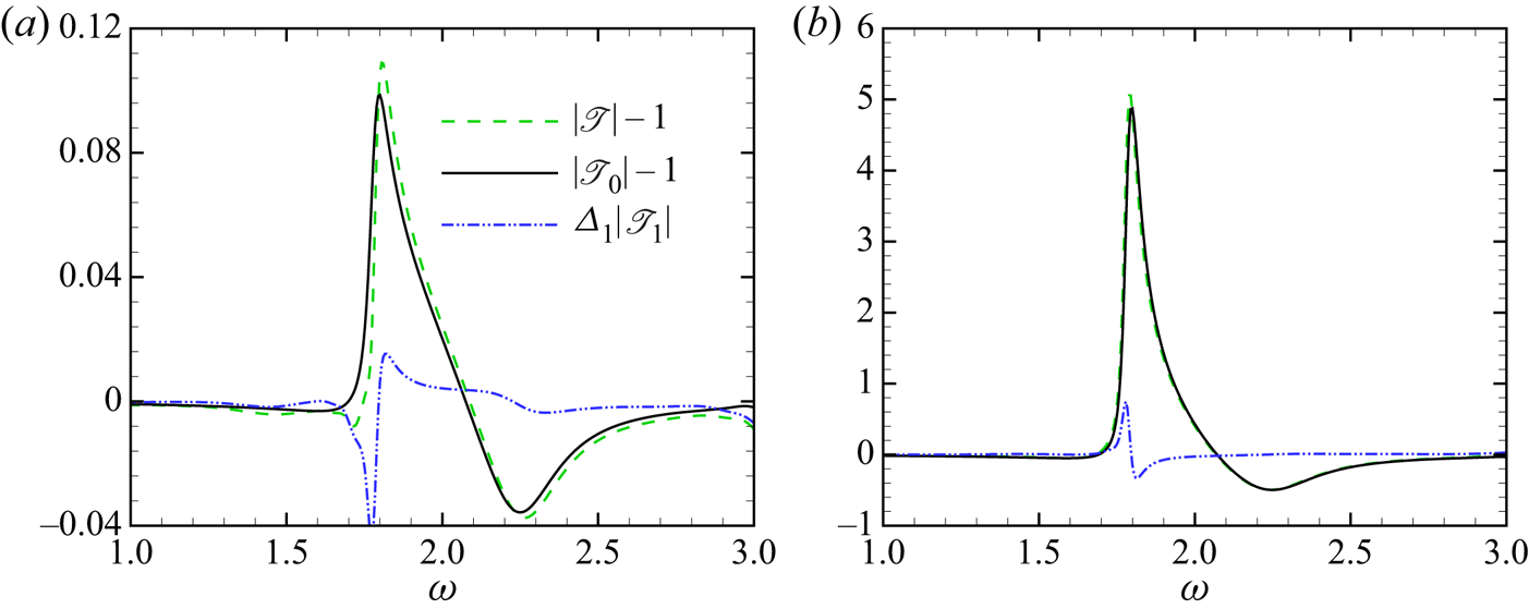
As indicated by (2.39), the transmission coefficient is contributed to by two orders, which are calculated by (2.32) and (2.37), respectively. Figure 17 plots the budget of the two contributors,  $|{\mathscr {T}}_0|-1$ and
 $\varDelta _1|{\mathscr {T}}_1|$, for two representative cases obtained by the improved asymptotic theory. For a small hump height, shown in panel (a), the transmission coefficient is close to unity, indicating that (2.42) is also a good approximation of
 $\mathscr {T}$. Therefore, the leading-order contributor,
 $|{\mathscr {T}}_0|-1$, is approximated by
 $K_{0,i}({\mathcal {D}}_1+h{\mathcal {D}}_2)$. The implication is that the trend of the dependence of
 $|{\mathscr {T}}_0|-1$ on
 $\omega$ is proportional to
 $K_{0,i}$, which can be seen by comparing with the green dashed line in figure 10(b). Its strength is determined by the level of the mean-flow distortion. For both panels, the second-order contributor,
 $\varDelta _1{\mathscr {T}}_1$, is always small except at
 $\omega \approx 1.8$, where the leading-order contributor also peaks. Thus, the second-order contributor may only have a limited impact in a narrow frequency band around this frequency.
Leading- and second-order contributors to the transmission coefficient obtained by the improved asymptotic theory, where (a,b) are for cases H1 and H4, respectively.

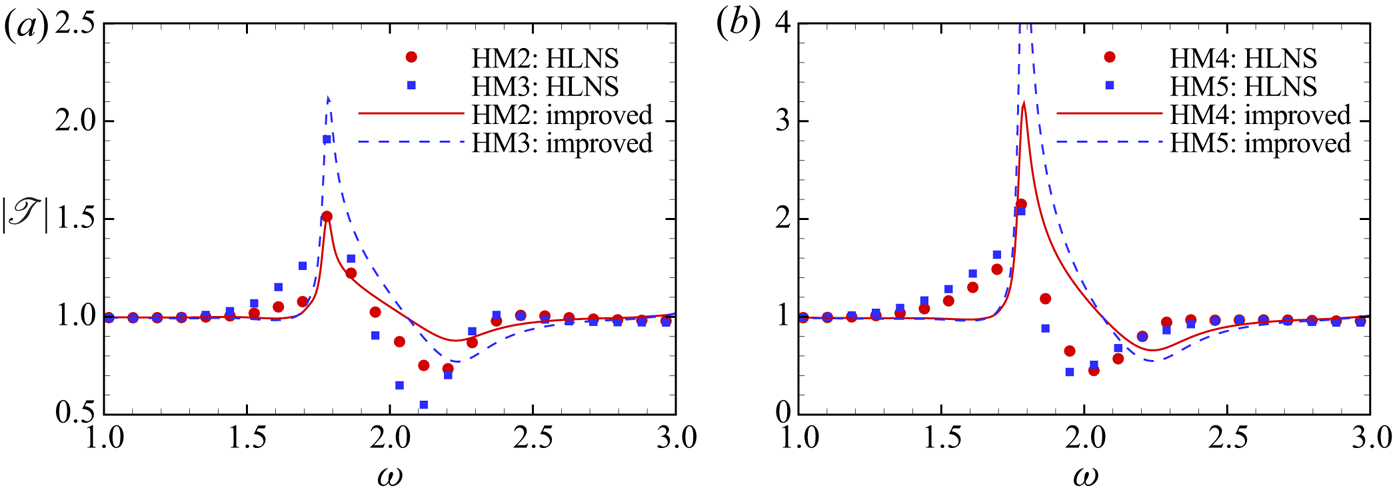
The comparison between the improved asymptotic predictions and HLNS calculations for indentation cases are shown in figure 18. For relatively shallow indentations, as shown in figure 18(a), the two results agree reasonably well, although the asymptotic theory under-predicts slightly the stabilising effect for supercritical frequencies. On the other hand, for deeper indentations ( $|h| \geqslant 0.20\delta _{99}$), the agreement becomes poorer, i.e. the improved theory over-predicts the destabilising effect in a narrow frequency band around
 $\omega =1.8$. The critical frequency calculated by the HLNS approach shows an appreciable decrease trend as the indentation depth increases, but that obtained by the asymptotic theory stays almost unchanged. This may be attributed to the impact of the second-order mean-flow distortion that is neglected (2.7), which could be relatively greater for deeper indentations.
Dependence of the norm of the transmission coefficient on frequency  $\omega$ for indentation cases (cases HM2 to HM5), where curves and symbols are for the improved asymptotic solutions and the HLNS calculations, respectively.

The displacement function  $A$ or
 $\tilde {A}$, representing the mean-flow distortion, is negative for humps, but positive for indentations, as shown in figure 9. However, both humps and indentations produce the same scattering effect, i.e. the stabilising effect for supercritical frequencies and destabilising effect for subcritical frequencies, which has been listed as the unexplained phenomenon (i) in the Introduction. Indeed, the asymptotic theory is able to explain this phenomenon clearly. From (2.32) we know that the leading-order scattering is determined by the product of
 $K_0$ and
 ${\mathcal {D}}_1+h{\mathcal {D}}_2$. The former is independent of the mean-flow distortion, and therefore is the same for the hump and indentation cases. The latter is proportional to
 $\bar {\mathcal {D}}_1+H\bar {\mathcal {D}}_2$, whose values for different cases can be found in table 2. It is easy to see that
 $\bar {\mathcal {D}}_1$ and
 $H\bar {\mathcal {D}}_2$ have opposite signs, and the scattering effect is determined by their comprehensive effects. For nonlinear hump cases,
 $\bar {\mathcal {D}}_1$ is negative, and
 $|\bar {\mathcal {D}}_1|>|H\bar {\mathcal {D}}_2|$, implying that
 $\bar {\mathcal {D}}_1+H\bar {\mathcal {D}}_2<0$. For nonlinear indentation cases,
 $\bar {\mathcal {D}}_1$ is positive but smaller than
 $|H \bar {\mathcal {D}}_2|$, leading to
 $\bar {\mathcal {D}}_1+H\bar {\mathcal {D}}_2<0$ also. Consequently, the destabilising and stabilising effects would be observed in the same frequency band.
 $|\bar {\mathcal {D}}_1+H\bar {\mathcal {D}}_2|$ is greater for a hump than that for an indentation with the same
 $|h|$ or
 $|H|$, implying that the scattering effect of a nonlinear indentation is always weaker.
4.4.3. Comparison with the HLNS results for a moderate Reynolds number
The error of the asymptotic theories is mainly attributed to two factors: (a) the discrepancy of the mean-flow distortion between the triple-deck theory and DNS calculations, and (b) the discrepancy of the (improved) Rayleigh and O–S operators. Both factors lead to a greater error as  $R$ decreases. In this subsection, we choose the Reynolds number
 $R=26\,364$, which is the same as that of case 1 in Zhao et al. (Reference Zhao, Dong and Yang2019). Note that, in that paper, the Reynolds number
 $Re$ was defined as
 $U_\infty L/\nu _\infty$, which is related to the present Reynolds number
 $R$ via
 $Re=R^{2}/\varDelta ^{2}$.
Figure 11(a,b) of Zhao et al. (Reference Zhao, Dong and Yang2019) shows the dependence of the transmission coefficient on frequency for different heights  $h^{*}/\delta _{99}$ and widths
 $d^{*}/\delta _{99}$, respectively. We carry out calculations by the improved asymptotic theory for the same parameters, and the comparisons are shown in figure 19. Both families of curves exhibit a critical frequency at
 $\omega \approx 2$, which distinguishes the stabilising and destabilising effects of the humps. The overall trends agree well, despite the fact that the asymptotic theory over-predicts quantitatively the destabilising effect in the frequency band
 $1.6< \omega < 2$ and under-predicts the stabilising effect in supercritical frequencies.
Dependence of the norm of the transmission coefficients on frequency  $\omega$ for
 $R=26\,364$. (a) Fixed
 $d^{*}/\delta _{99}=2$ with
 $h^{*}/\delta _{99}=0.05$ (red), 0.1 (green), 0.15 (blue), 0.2 (purple) and 0.25 (black); (b) fixed
 $h^{*}/\delta _{99}=0.25$ with
 $d^{*}/\delta _{99}=2$ (black), 4 (red), 6 (green) and 8 (blue). Solid lines: the asymptotic predictions; circles: the HLNS calculations.

Admittedly, the error due to the finite- $R$ effect should be greater than that in the previous subsection, and the narrow width
 $d^{*}/\delta _{99}=2$ may also lead to a poorer prediction of the mean-flow distortion. However, the asymptotic theory can still predict the HLNS results with a satisfactory accuracy. The reason is that, whether the roughness plays a stabilising or destabilising role is indeed determined by the Rayleigh operator governing the property of the perturbation, which is independent of the mean-flow distortion and is affected weakly by the finite-
 $R$ and narrow-roughness effects, as is indicated by figure 5. On the other hand, the intensity of the scattering effect is related to the mean-flow calculation, the error of which may be attributed to both the finite-
 $R$ effect and the narrow-roughness effect. However, the two effects seem to be in the opposite directions, and due to the cancellation effect, the error of the improved asymptotic theory does not increase to an unacceptable state.
One may query why the scattering effect seems to be unchanged as the roughness width increases in figure 19(b), which is the unexplained phenomenon (iii) as listed in the Introduction. According to the triple-deck formalism, the roughness heights for the cases in figure 19(b) are all converted to  $H=1.24$, while their widths are converted to
 $D=0.351$, 0.702, 1.05 and 1.40, respectively. Figure 20 shows
 $\bar {\mathcal {D}}_1$ and
 $H\bar {\mathcal {D}}_2$, and their summation. As
 $D$ increases,
 $\bar {\mathcal {D}}_1$ decreases, while
 $H\bar {\mathcal {D}}_2$ increases. Interestingly, the sum of the two stays almost unchanged for different
 $D$, and so the leading-order scattering effect is almost independent of the roughness width.
Variations of  $\bar {\mathcal {D}}_1+H\bar {\mathcal {D}}_2$ (red solid line),
 $\bar {\mathcal {D}}_1$ (green dashed line) and
 $H\bar {\mathcal {D}}_2$ (blue dot-dashed line) with roughness width
 $D$, where
 $H=1.24$.

Now let us compare the transmission coefficient for the same dimensionless roughness size, but different Reynolds numbers. The results in figure 16(i) and the blue curves in figure 19(b) are both for  $h^{*}/\delta _{99}=0.25$ and
 $d^{*}/\delta _{99}=8$, but the Reynolds numbers are
 $R=131\,820$ and 26 364, respectively. For a fixed dimensionless frequency, the scattering effect, measured by
 $|{\mathscr {T}}-1|$, for the larger
 $R$ is much greater than that for the smaller
 $R$, which is listed as the unexplained phenomenon (ii) in the introduction part. For the same frequency, the factor
 $K_0$ is the same for the two Reynolds numbers, and the scattering effect essentially depends on
 ${\mathcal {D}}_1+ h{\mathcal {D}}_2$. According to (B2),
 ${\mathcal {R}}_X$ and
 ${\mathcal {R}}_Y$ are also the same for the same oncoming condition, then the key factor is
 $\bar {\mathcal {D}}_1+ H\bar {\mathcal {D}}_2$. Table 3 compares the key parameters for the two Reynolds numbers. For the same
 $h^{*}/\delta _{99}$ and
 $d^{*}/\delta _{99}$, as
 $R$ increases five times,
 $h$ and
 $H$ increase
 $5^{1/4}$ times, while
 $d$ and
 $D$ decrease
 $5^{-1/4}$ times. As a consequence,
 $HD$ does not change, neither does
 $H\bar {\mathcal {D}}_2$. However,
 $|\bar {\mathcal {D}}_1|$ increases remarkably with
 $R$, leading to a much greater mean-flow distortion. This is why the scattering effect increases with
 $R$.
Comparison of the key parameters for the two Reynolds numbers.

4.4.4. Impact of Mach number on the efficiency function
In fact, the scattering efficiency is affected by the Mach number, wall temperature, Reynolds number and frequency of the oncoming Mack mode. The above analysis has revealed the effects of the latter two factors by choosing  $(M,T_w)=(5.92,6.95)$. In this subsection, we select another group of control parameters, i.e.
 $(M,T_w)=(4.5,4.4)$, and study the dependence of the scattering effect on
 $\omega$ for
 $R=10\,400$ and 104 000. These parameters are selected from Ma & Zhong (Reference Ma and Zhong2003a,b) and case 1 of Dong et al. (Reference Dong, Liu and Wu2020), and the wall temperature is close to the adiabatic temperature at this
 $M$.
Figure 21 compares the phase speeds and growth rates obtained by the improved Rayleigh equations (symbols) and the O–S equations (curves). The phase speed calculated by the two approaches agree well, but the growth rates show apparent discrepancy. Increase of  $R$ leads to a reduction of the difference, which agrees with the observation for
 $M=5.92$. Being different from the case for
 $M=5.92$, the first and second modes for
 $M=4.5$ are separated in two different frequency bands. Therefore, near the first-mode upper-branch and second-mode lower-branch neutral frequencies, the Rayleigh equations become singular. In order to avoid the singularity, we employed the standard method as in Dong et al. (Reference Dong, Liu and Wu2020), namely, the integration path around the critical point, where the mean-flow velocity is equal to the phase speed, is detoured by adding a negative imaginary part to
 $y$ and extending the mean flow to the complex plane. In panel (a), the synchronisation frequencies for the two Reynolds numbers are also marked, which are
 $\omega _c\approx 1.87$ and 1.93, respectively.
Dependence of the phase speed  $c_r$ (a) and the growth rate
 $-\alpha _i$ (b) of 2-D Mack modes on the frequency
 $\omega\ {\rm for}\ (M,T_w=(4.5,4.4))$. Red solid lines: O–S solution for
 $R=10\,400$; blue dashed lines: O–S solution for
 $R=104\,000$; red circles: improved Rayleigh solution for
 $R=10\,400$; blue squares: improved Rayleigh solution for
 $R=104\,000$.

Figure 22 shows the efficiency frequency  $K_0$ for the two Reynolds numbers. The overall behaviour is the same as that in figure 10(a,b), i.e.
 $K_0$ shows a remarkable variation in the frequency band
 $1.5<\omega <2.5$, which includes the second-mode band and a portion of the stable-mode band;
 $K_{0,i}$ crosses zero at a frequency
 $\bar {\omega }_c$ which is close to the synchronisation frequency;
 $K_{0,i}<0$ for subcritical frequencies and
 $>0$ for supercritical frequencies. As
 $R$ increases, the maximum of
 $|K_{0,i}|$ becomes greater and
 $\bar {\omega }_c$ becomes higher. Comparing figure 22(b) with figure 10(b), we obtain that for similar Reynolds numbers (
 ${\approx }10^{5}$), as
 $M$ decreases, the maximum of
 $|K_{0,i}|$ increases, indicating a stronger scattering effect.
Dependence of the efficiency function  $K_0$ on frequency for
 $(M,T_w=(4.5,4.4))$. The thin horizontal line in (b) represents the zero line, and
 $\bar \omega _c$ represents the critical frequency for which
 $K_{0,i}$ crosses zero.

5. Concluding remarks and discussion
In the present paper, we developed an asymptotic theory to describe the impact of roughness on the oncoming inviscid first and second Mack modes in supersonic/hypersonic boundary layers. For analytical convenience, the height of the roughness is assumed to be much lower than the local boundary-layer thickness, and its width is assumed to be much longer than the latter. This is a multi-scale problem because in the streamwise direction the Mack wavelength is much shorter than the roughness width, while the length scale of the non-parallelism of the Blasius solution is much wider. As the Reynolds number is asymptotically large, the mean-flow distortion induced by the roughness can be described by the triple-deck formalism (Stewartson Reference Stewartson1969; Messiter Reference Messiter1970; Smith Reference Smith1973), and the inviscid Mack mode exhibits a double-layered structure, a main layer and a near-wall Stokes layer. Their interaction is described by the multi-scale analysis. The scattering effect is quantified by a transmission coefficient (Wu & Dong Reference Wu and Dong2016b), defined as the amplitude of the Mack mode downstream of the roughness to that upstream.
From the asymptotic theory, the impacts of the mean-flow distortion and the instability property of the oncoming Mack mode are readily separated. To leading order, whether the roughness plays a stabilising or destabilising role is determined by an efficiency function  $K_{0,i}$. It is found that
 $K_{0,i}$ varies remarkably in most of the second-mode frequency band and a small portion of the first-mode frequency band. It crosses zero from negative to positive as the frequency increases to a critical frequency, which distinguishes the stabilising and destabilising effects. The appearance of the critical frequency is analysed in § 4.4.1. The critical frequency is close to the synchronisation frequency, in agreement with the numerical observations of Fong et al. (Reference Fong, Wang and Zhong2014, Reference Fong, Wang and Zhong2015b) and Zhao et al. (Reference Zhao, Dong and Yang2019). The intensity of the leading-order stabilising or destabilising effect, on the other hand, depends on the height and/or width of the roughness, which is attributed to two factors: (i) the interaction between the roughness-induced mean-flow distortion and the oncoming Mack mode in the main deck,
 ${\mathcal {D}}_1K_0$, and (ii) the inhomogeneous forcing from the curved wall (Stokes layer),
 $h{\mathcal {D}}_2K_0$. Interestingly, the impacts of these two factors are always in the opposite directions, and the comprehensive scattering effect is due to their competition. In the low-roughness limit,
 $|h|\ll R^{-1/4}$, the two factors are exactly opposite to each other, and so the roughness has no effect on oncoming inviscid Mack modes to leading order, i.e.
 ${\mathscr {T}}_0=1$. For a nonlinear hump with
 $h=O(R^{-1/4})$,
 ${\mathcal {D}}_1$ is negative, and its absolute value is greater than
 $h{\mathcal {D}}_2$. The consequence is that the hump plays a destabilising/stabilising role for subcritical/supercritical frequencies. For a nonlinear indentation with
 $-h=O(R^{-1/4})$,
 ${\mathcal {D}}_1$ is positive, which, however, is smaller than
 $|h|{\mathcal {D}}_2$. Therefore, the indentation also enhances/suppresses the oncoming Mack modes for subcritical/supercritical frequencies, but this effect is usually weaker than that of the hump with the same
 $|h|$. The scattering effect, measured by
 $|{\mathscr {T}}|-1$, increases with the roughness height
 $h$ monotonically, but changes only mildly as the roughness width increases; see figure 19(b). The explanation is as follows: for a fixed roughness height,
 $\bar {\mathcal {D}}_1$ decreases with
 $D$, while
 $H\bar {\mathcal {D}}_2$ increases with
 $D$; their sum leads to an almost unchanged value,
 $\bar {\mathcal {D}}_1+H\bar {\mathcal {D}}_2$, rendering an almost independent nature of the scattering effect on the roughness width. For a fixed dimensionless roughness shape and Mack-mode frequency, the scattering effect becomes stronger as the Reynolds number increases. The reason is that the normalised height
 $H$ increases like
 $R^{1/4}$ while the normalised width
 $D$ decreases like
 $R^{-1/4}$; increase of
 $R$ would lead to a greater
 $\bar {\mathcal {D}}_1$ but the unchanged
 $H\bar {\mathcal {D}}_2$, leading to an increase of the scattering effect. Additionally, increase of the Mach number leads to a decrease of the scattering effect.
The second-order scattering is associated with the interaction between the non-parallelism of the oncoming Mack modes and the roughness-induced mean-flow distortion. Due to its small magnitude, its impact on the transmission coefficient is usually rather weak. Only a small impact is observed at the intersection frequency of the first and second modes. The second-order scattering effect leads to a mild variation of the perturbation amplitude in relevant to that of the smooth-surface configuration in the downstream limit, which agrees with the numerical observations.
In order to increase the accuracy of the asymptotic prediction, we also developed an improved asymptotic theory by taking into account the impact of the viscous Stokes layer. Although its impact is only of  $O(R^{-1/2})$, it is found that the improved theory can increase remarkably the accuracy of the prediction of the growth rate at a moderate Reynolds number as compared with the O–S solution, especially in the frequency band near the intersection of the first and second modes. Actually, the original asymptotic predictions for the amplitude correction are almost infinite in this band, because near the frequency for which the growth rate reaches its minimum, the eigensolutions of the streamwise velocity and temperature obtained by the Rayleigh equation are almost singular. However, the improved theory provides a rather reasonable prediction in this frequency band. In this paper, we also carry out numerical calculations by DNS and HLNS approaches, the results of which agree perfectly. Both the norms and phase angles of the transmission coefficients predicted by the asymptotic theory agree overall with those by numerical calculations for a large and a moderate Reynolds numbers. Satisfactory agreements are achieved even when the roughness height is a quarter of the nominal boundary-layer thickness.
Indeed, the scattering process discussed in this paper is a non-resonant regime, and the amplitude evolution  $C(X)$ is the accumulation of the growth-rate correction of the oncoming Mack mode induced by the wide-roughness element. The correction of the growth rate is merely of
 $O(R^{-1/4})$, but integral interval is as long as
 $O(R^{1/4})$, leading to an
 $O(1)$ scattering effect. If the roughness width is decreased to be comparable with the wavelength of the Mack modes, then the resonant regime appears. One may develop an asymptotic theory on describing the mean-flow distortion induced by narrow roughness if the roughness height is reduced to of
 $O(R^{-1/3})$; see Dong et al. (Reference Dong, Liu and Wu2020). The latter was focusing on the local receptivity of the inviscid Mack modes due to the sound–roughness interaction, but this theory can also describe the local scattering regime by replacing the incident acoustic wave by the oncoming Mack mode. Following that paper, we know that the Stokes layer driven by the oncoming Mack mode is distorted by the curved wall near the narrow roughness, which leads to the leading-order scattering effect, while the interaction between the mean-flow distortion and the oncoming mode is the second-order contributor. Interesting enough, we can show that the present theory could recover the resonant regime of Dong et al. (Reference Dong, Liu and Wu2020) in the narrow-roughness limit. If the roughness width approaches the boundary-layer thickness
 $\delta _{99}$, then the triple-deck width
 $D\rightarrow \epsilon$, which, according to Smith et al. (Reference Smith, Brighton, Jackson and Hunt1981), leads to
 $\tilde {A}\rightarrow 0$. Therefore, the leading-order scattering is determined only by
 $K_0h{\mathcal {D}}_2$, and the interaction of the Mack mode with the roughness-induced mean-flow distortion,
 $K_0{\mathcal {D}}_1$, becomes the second-order impact, in agreement with the resonant regime. Note that here the height of the roughness is assumed to be at most of
 $O(R^{-1/3})$ because the wall layer for a narrow-roughness element is thinner. Remarkably, if the roughness is sufficiently narrow and low, the overall trend of the scattering effect would be changed to the opposite direction, i.e. the stabilising effect appears in the subcritical frequency band, whereas the destabilising effect appears for supercritical frequencies. However, because of the inhomogeneous forcing from the curved wall (Stokes layer) is weak for a low roughness, the transmission coefficient would be rather close to unity, which is not easy to be seen in DNS or HLNS results due to the contamination of the numerical noises.
Acknowledgements
The authors would like to thank Professor X. Wu of Imperial College London for his valuable comments and suggestions.
Funding
The work is supported by National Science Foundation of China (grant nos. U20B2003, 11772224, 12002235, 91952202).
Declaration of interests
The authors report no conflict of interest.
Appendix A. Outer-region solution for  $\bar {x}\rightarrow 0$

In the region where  $\bar {x}=O(1)$ and
 $y=O(1)$, the impact of the roughness is negligible, and the mean flow satisfies the non-parallel Blasius solution. As
 $\bar {x}\rightarrow 0$, the mean flow is expanded as
 \begin{equation} \bar{\boldsymbol\varphi}=\bar{\boldsymbol\varphi}_B+\bar{x} \bar{\boldsymbol\varphi}_{B,\bar{x}}+\cdots, \end{equation}
where  ${\boldsymbol\varphi} _B$ denotes the Blasius solution at
 $\bar {x}=0$. The infinitesimal perturbation is expanded as
 \begin{align} {\mathcal{E}}(\tilde{\boldsymbol\phi}_0(\bar{x},y)+\epsilon\varDelta_1\tilde{\boldsymbol\phi}_1(\bar{x},y)+\cdots) \exp\left({{\textrm{i}}\left[\epsilon^{{-}1}\varDelta_1^{{-}1}\int\alpha(\bar{x}) \ \textrm{d}\bar{x}+\beta z-\omega t\right]}\right)+\textrm{c.c.}, \end{align}
where
 \begin{equation} \tilde{\boldsymbol\phi}_0=\bar{C}(\bar{x})(\hat{\boldsymbol\phi}(y;\bar{x}=0)+\bar{x}\hat{\boldsymbol\phi}_{\bar{x}}(y;\bar{x}=0)+\cdots), \end{equation}
with  $\bar {C}(\bar {x})$ being the perturbation amplitude.
Substituting (A2) with (A3) into (2.2), we obtain that the leading-order perturbation is governed by the Rayleigh equation (2.14), while the second-order perturbation is governed by
 \begin{equation} {\mathcal{L}}_R\tilde{\boldsymbol\phi}_1={-}{\textrm{i}}\frac{\partial {{\boldsymbol{\mathsf{H}}}}_0}{\partial \alpha}(\bar{C}'\hat{\boldsymbol\phi}+\bar{C}\hat{\boldsymbol\phi}_{\bar{x}})+{{\boldsymbol{\mathsf{H}}}}_2\bar{C}\hat{\boldsymbol\phi}, \end{equation}
where
 \begin{equation} {{\boldsymbol{\mathsf{H}}}}_2=\left( \begin{array}{cc} {{\boldsymbol{\mathsf{H}}}}_{2,11} & {{\boldsymbol{\mathsf{H}}}}_{2,12} \\ {{\boldsymbol{\mathsf{H}}}}_{2,21} & 0 \end{array} \right) \end{equation}
with  $S_0={\textrm {i}}\alpha (U_B-c)$, and
 \begin{equation}
\left.\begin{gathered}
{{\boldsymbol{\mathsf{H}}}}_{2,11}=\left(\frac{{\textrm{i}}\alpha S_0
U_2'+ \alpha^{2}U_B'U_2}{S_0^{2}}\right)X \\
\quad+\left(\frac{{\textrm{i}}\alpha(U_BT_B'-T_BU_B')}{S_0^{2}T_B}-\frac{T_B'}{\gamma
S_0T_B}\right)U_2-\frac{T_B'U_B}{\gamma S_0T_B^{2}}T_2,\\
{{\boldsymbol{\mathsf{H}}}}_{2,12}=\left[-\frac{\tilde\alpha^{2}T_2}{S_0}+{\textrm{i}}\alpha
U_2\left(\frac{\tilde{\alpha}^{2}T_B}{S_0^{2}}-M^{2}
\right)\right]X-\frac{M^{2}U_B}{\gamma T_B}T_2\\
\quad +\left[\frac{\tilde\alpha^{2}T_B+{\textrm{i}}\alpha
M^{2}S_0U_B}{S_0^{2}}-\left(\gamma-1+\frac
1\gamma\right)M^{2}\right]U_2,\\
{{\boldsymbol{\mathsf{H}}}}_{2,21}=\left(\frac{S_0T_2}{T_B^{2}}-\frac{{\textrm{i}}\alpha
U_2}{T_B}\right)X. \end{gathered}\right\}
\end{equation}
Multiplying both sides of (A4) by the adjoint vector  $\hat{\boldsymbol\phi}^{{\dagger} }$ and integrating from 0 to
 $\infty$, we obtain the amplitude equation
 \begin{equation} {\textrm{i}}\bar{C}'(\bar{x})=\left(-{\textrm{i}}K_2+K_4\right)\bar{C}(\bar{x}). \end{equation}
The solution is
 \begin{equation} \bar{C}(\bar{x})=D_0\exp({({-}K_2-{\textrm{i}}K_4)\bar{x}}), \end{equation}
where  $D_0$ is a constant. For
 $\bar {x}\rightarrow 0^{\pm }$, (A8) is recast to
 \begin{equation} \bar{C}(\bar{x})=1+D_0^{{\pm}}({-}K_2-{\textrm{i}}K_4)\bar{x}+\cdots. \end{equation}
Matching with the inner-region solution (2.34), we obtain
 \begin{equation} D_0^{-}=1,\quad D_0^{+}={\mathscr{T}}_0. \end{equation}
Appendix B. Lower-deck analysis of the roughness-distorted mean flow
B.1. Equation system
The mean-flow distortion induced by the roughness is described by the triple-deck formalism (Stewartson Reference Stewartson1969; Messiter Reference Messiter1970; Smith Reference Smith1973). Here, for brevity, we skip the mathematical details and directly go to the conclusion.
In the lower deck, where  $Y=\epsilon ^{-1}y=O(1)$, we re-normalise the coordinates as
 \begin{equation} \tilde{X}={\mathcal{R}}_XX,\quad\breve{Y}={\mathcal{R}}_YY, \end{equation}
where
 \begin{equation} {\mathcal{R}}_X=\lambda^{5/4}(M^{2}-1)^{3/8}\bar{C}^{{-}3/8}T_w^{{-}3/2},\quad {\mathcal{R}}_Y=\lambda^{3/4}(M^{2}-1)^{1/8}\bar{C}^{{-}5/8}T_w^{{-}3/2}, \end{equation}
with  $\lambda =\bar {C}^{1/2}T_wU_{B,y}(0)$ being the wall shear of the Blasius profile and
 $\bar {C}=\mu (T_w)/T_w$. The roughness height and width are re-scaled as
 \begin{equation} H={\mathcal{R}}_Yh,\quad D={\mathcal{R}}_Xd. \end{equation}
According to (B1a,b), the roughness shape function (2.6) is recast to
 \begin{equation} f(\tilde{X})=
\begin{cases} \displaystyle\tfrac 12[1+\cos(2{\rm \pi}
\tilde{X}/ D)] & \mbox{for }|\tilde{X}| \leqslant
D/2,\\ 0 & \mbox{otherwise}. \end{cases}
\end{equation}
The velocity field and pressure are re-scaled as
 \begin{equation} \tilde{U}=\epsilon^{{-}1}{\mathcal{R}}_U \bar{U},\quad \breve{V}=\epsilon^{{-}3}{\mathcal{R}}_V \bar{V},\quad \tilde{P}=\epsilon^{{-}2}{\mathcal{R}}_P (\bar{P}-1/(\gamma M^{2})), \end{equation}
where
 \begin{equation} \left\{\begin{array}{l} \displaystyle{\mathcal{R}}_U=\lambda^{{-}1/4}(M^{2}-1)^{1/8}\bar{C}^{{-}1/8}T_w^{{-}1/2}, \\ \displaystyle{\mathcal{R}}_V=\lambda^{{-}3/4}(M^{2}-1)^{1/8}\bar{C}^{{-}3/8}T_w^{{-}1/2}, \\ \displaystyle{\mathcal{R}}_P=\lambda^{{-}1/2}(M^{2}-1)^{1/4}\bar{C}^{{-}1/4}. \end{array}\right. \end{equation}
In order to regularise the computational domain to be rectangular, the Prandtl transformation is employed,
 \begin{equation} \tilde{Y}=\breve{Y}-Hf,\quad \tilde{V}=\breve{V}+\tilde{U}H\,f_{\tilde{X}}. \end{equation}
Substituting the re-scaled coordinates and flow field into the N–S equations and retaining the leading-order terms, we obtain the incompressible boundary-layer equations,
 \begin{equation} \tilde{U}_{\tilde{X}}+\tilde{V}_{\tilde{Y}}=0,\quad \tilde{U}\tilde{U}_{\tilde{X}}+\tilde{V} \tilde{U}_{\tilde{Y}}={-}\tilde{P}_{\tilde{X}}+\tilde{U}_{\tilde{Y}\tilde{Y}}, \end{equation}
which are subject to the boundary and matching conditions
 \begin{equation} \tilde{U}(\tilde{X},0)=\tilde{V}(\tilde{X},0)=0,\quad\tilde{U}(\tilde{X},\tilde{Y})\rightarrow \tilde{Y}+Hf(\tilde{X})+\tilde{A}\quad\mbox{as }\tilde{Y}\rightarrow \infty, \end{equation}
where  $\tilde {A}$ is the re-scaled displacement function.
 $\tilde {A}$ is related to
 $A$ (defined in § 2.3.1) via
 \begin{equation} \tilde{A}={\mathcal{R}}_YA. \end{equation}
Matching the lower-deck solution with the upper-deck solution through the main deck, we obtain the supersonic pressure–displacement relation,
 \begin{equation} \tilde{P}(X)={-}\tilde{A}_{\tilde{X}}(\tilde{X}). \end{equation}
The above system can be solved numerically by the same method as that in Wu & Dong (Reference Wu and Dong2016b), with only a modification of the pressure–displacement relation. In the numerical calculations, we select the computational domain as  $[-20,30]\times [0,15]$ and the number of grid points as
 $521\times 51$.
B.2. Analytical solutions of the triple-deck system for $H\ll 1$

In the low-roughness limit, we seek analytical solutions of  $\tilde {U}$,
 $\breve {V}$ and
 $\tilde {P}$ in the coordinate system
 $(\tilde {X},\breve {Y})$. The Prandtl transformation is not needed. The governing equations of
 $\tilde {U}$,
 $\breve {V}$ and
 $\tilde {P}$ remain the same as (B8a,b) and (B11). For
 $H\ll 1$, we can express the solutions in terms of asymptotic series,
 \begin{equation} (\tilde{U},\breve{V},\tilde{P},\tilde{A})=(\breve{Y},0,0,0)+H\left(\tilde{u}_M,\tilde{v}_M,\tilde{p}_M, \tilde{a}_M\right)+O(H^{2}), \end{equation}
where the first term on the right-hand side denotes the Blasius solution. Substituting (B12) into the governing equations and performing a Fourier transform with respect to  $\tilde {X}$, we obtain
 \begin{equation} {\textrm{i}} \tilde{k}\hat{u}_M+\hat{v}_M'=0,\quad {\textrm{i}}\tilde{k}\breve{Y} \hat{u}_M+\hat{v}_M={-}{\textrm{i}}\tilde{k}\hat{p}_M+\hat{u}_M'',\quad \hat{p}_M={-}{\textrm{i}}\tilde{k}\hat{a}_{M}, \end{equation}
where
 \begin{equation} (\hat{u}_M,\hat{v}_M,\hat{p}_M,\hat{a}_M)(\breve{Y};\tilde{k})=\int_{-\infty}^{\infty} \left(\tilde{u}_M,\tilde{v}_M,\tilde{p}_M,\tilde{a}_M\right){\textrm{e}}^{-{\textrm{i}}\tilde{k}\tilde{X}} \ \textrm{d}\tilde{X}. \end{equation}
The boundary conditions read
 \begin{equation} (\hat{u}_M(0),\hat{v}_M(0))=(-\hat{f}(0),0),\quad \hat{u}_M(\breve{Y})\rightarrow \hat{a}_M\quad\mbox{as }\breve{Y}\rightarrow\infty. \end{equation}
Following Smith (Reference Smith1973), it is obtained that, for  $\tilde {k}\ne 0$, the solution is
 \begin{equation} \hat{u}_M(\breve{Y};\tilde{k})=\hat{f}(\tilde{k})\left(\frac{\displaystyle\int_0^{({\rm i} \tilde{k})^{1/3}\breve{Y}} \mbox{Ai}(\hat{\xi})\, \textrm{d}\hat\xi}{\displaystyle\int_0^{\infty}\mbox{Ai}(\hat{\xi})\ \textrm{d}\hat{\xi}+({\textrm{i}}\tilde{k})^{{-}4/3}\mbox{Ai}'(0)}-1\right), \end{equation}
where  $\hat {f}(\tilde {k})=\int _{-\infty }^{\infty } f(\tilde {X})\,{\textrm {e}}^{-{\textrm {i}}\tilde {k}\tilde {X}} \ \textrm {d}\tilde {X}$. For
 $\tilde {k}=0$, the solution is
 \begin{equation} \hat{u}_M(\breve{Y})=\hat{a}_M(0)={-}\hat{f}(0). \end{equation}
Therefore, for a sufficiently low roughness, we have
 \begin{equation} \int_{-\infty}^{\infty} \tilde{A}(\tilde{X})\ \textrm{d}\tilde{X}={-}H\hat{f}(0)={-}H\int_{-\infty}^{\infty} f(\tilde{X})\ \textrm{d}\tilde{X}, \end{equation}
implying that the leading-order transmission coefficient, according to (2.32), is unity. The equation also indicates that the displacement function has an opposite sign to  $f$, namely,
 $\int_{-\infty}^\infty \tilde A(\tilde X) {\rm d}\tilde X$ is negative for a hump and positive for an indentation.
Appendix C. Proof for $K_0=K_1$

Since  $K_0$ and
 $K_1$ have the same denominator, we will prove that their numerators are equal. Using the definition (2.28a,b) and the relation (2.17b), and performing integration by parts, the numerator of
 $K_0$ is recast to
 \begin{align} \langle\hat{\boldsymbol\phi}^{{\dagger}ger},{{\boldsymbol{\mathsf{H}}}}_1\hat{\boldsymbol\phi}\rangle&= \int_0^{\infty} (\hat{\boldsymbol\phi}^{{\dagger}ger})^\textrm{T}{{\boldsymbol{\mathsf{H}}}}_1\hat{\boldsymbol\phi}\, {\textrm{d} y}= \int_0^{\infty} (\hat{\boldsymbol\phi}^{{\dagger}ger})^\textrm{T}\left({{\boldsymbol{\mathsf{H}}}}_0\right)'\hat{\boldsymbol\phi} \,{\textrm{d} y} = \int_0^{\infty} \hat{\boldsymbol\phi}^{T}({{\boldsymbol{\mathsf{H}}}}_0^{T})'\hat{\boldsymbol\phi}^{{\dagger}ger} \,{\textrm{d} y} \nonumber\\ &=\int_0^{\infty} \hat{\boldsymbol\phi}^{T}[({{\boldsymbol{\mathsf{H}}}}_0^{T}\hat{\boldsymbol\phi}^{{\dagger}ger})'-{{\boldsymbol{\mathsf{H}}}}_0^{T} (\hat{\boldsymbol\phi}^{{\dagger}ger})']{\textrm{d} y}\nonumber\\ &=\left[\hat{\boldsymbol\phi}^{T}\boldsymbol{\mathsf{H}}_0^{T}\hat{\boldsymbol\phi}^{{\dagger}ger}-\int_0^{\infty}(\hat{\boldsymbol\phi}')^\textrm{T} {{\boldsymbol{\mathsf{H}}}}_0^{T}\hat{\boldsymbol\phi}^{{\dagger}ger} \,{\textrm{d} y}\right] -\left[\hat{\boldsymbol\phi}^{T}\boldsymbol{\mathsf{H}}_0^{T}\hat{\boldsymbol\phi}^{{\dagger}ger}-\int_0^{\infty} (({{\boldsymbol{\mathsf{H}}}}_0\hat{\boldsymbol\phi})')^\textrm{T} \hat{\boldsymbol\phi}^{{\dagger}ger} \,{\textrm{d} y}\right]\nonumber\\ & =\int_0^{\infty} [(\hat{\boldsymbol\phi}'')^\textrm{T} \hat{\boldsymbol\phi}^{{\dagger}ger} -(\hat{\boldsymbol\phi}')^\textrm{T}{{\boldsymbol{\mathsf{H}}}}_0^{T} \hat{\boldsymbol\phi}^{{\dagger}ger}]{\textrm{d} y}\nonumber\\ &=\left.(\hat{\boldsymbol\phi}^{{\dagger}ger})^\textrm{T}\hat{\boldsymbol\phi}'\right|_0^{\infty}-\int_0^{\infty} (\hat{\boldsymbol\phi}')^\textrm{T}[(\hat{\boldsymbol\phi}^{{\dagger}ger})' +{{\boldsymbol{\mathsf{H}}}}_0^{T} \hat{\boldsymbol\phi}^{{\dagger}ger}]{\textrm{d} y}=\left.-(\hat{\boldsymbol\phi}^{{\dagger}ger})^\textrm{T}\hat{\boldsymbol\phi}'\right|_{y=0}. \end{align}
Noting that  $\hat{\phi}^{{\dagger} }_{(2)}(0)=0$, the numerator of
 $K_1$ can be recast to
 \begin{equation} \langle\hat{\boldsymbol\phi}^{{\dagger}ger},\delta(y){\boldsymbol{\mathsf{H}}}\rangle= \hat{\boldsymbol\phi}^{{\dagger}ger}_{(1)}(0)(-\hat{v}'(0))=\left.-(\hat{\boldsymbol\phi}^{{\dagger}ger})^\textrm{T}\hat{\boldsymbol\phi}'\right|_{y=0}. \end{equation}
Thus, we obtain  $K_0=K_1$.