2 Experimental methods

A series of experiments were conducted in the free surface water channel (FSWC) of the Laboratory for Fluid–Structure Interactions (LIFE) at Universitat Rovira i Virgili (URV) in Tarragona. The water channel has a cross-section of $1\times 1.1~\text{m}^{2}$ downstream of a 6 to 1 (cross-sectional area) three-dimensional contraction, and is able to deliver over $0.6~\text{m}^{3}~\text{s}^{-1}$ . The flow is generated by two axial pumps controlled by two frequency sources, and the profile in the working section is characterised by very low variability in the velocity, with a maximum deviation in velocity of 1.58 %.

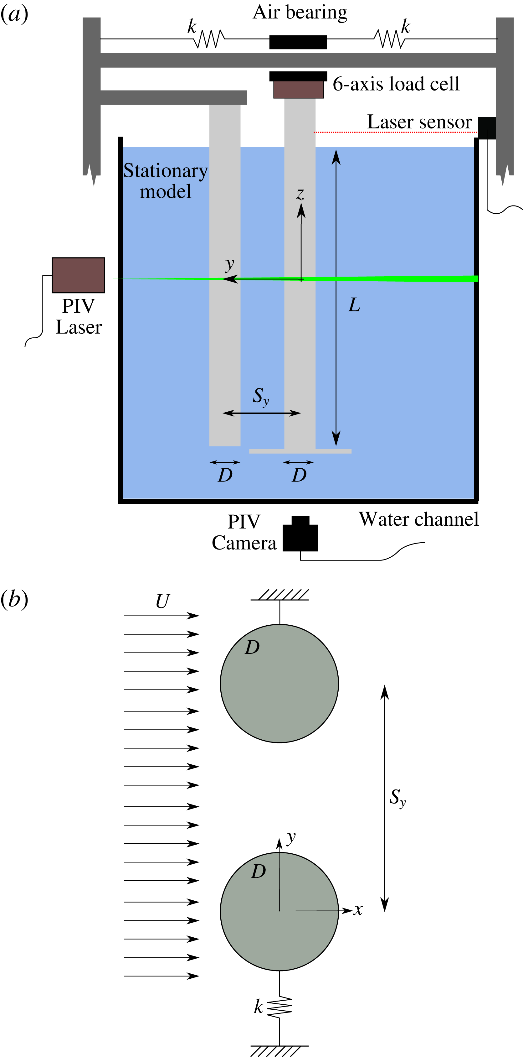
The experimental arrangement consisted of two rigid circular cylinders made of transparent acrylic tubes. They were installed on top of the channel, on a structure that is not in contact with it, so structural vibrations due to its operation were avoided. Both cylinder models had the same external diameter $D=0.05$  m and the same submerged length $L=0.5$  m, leading to an aspect ratio $L/D=10$ . 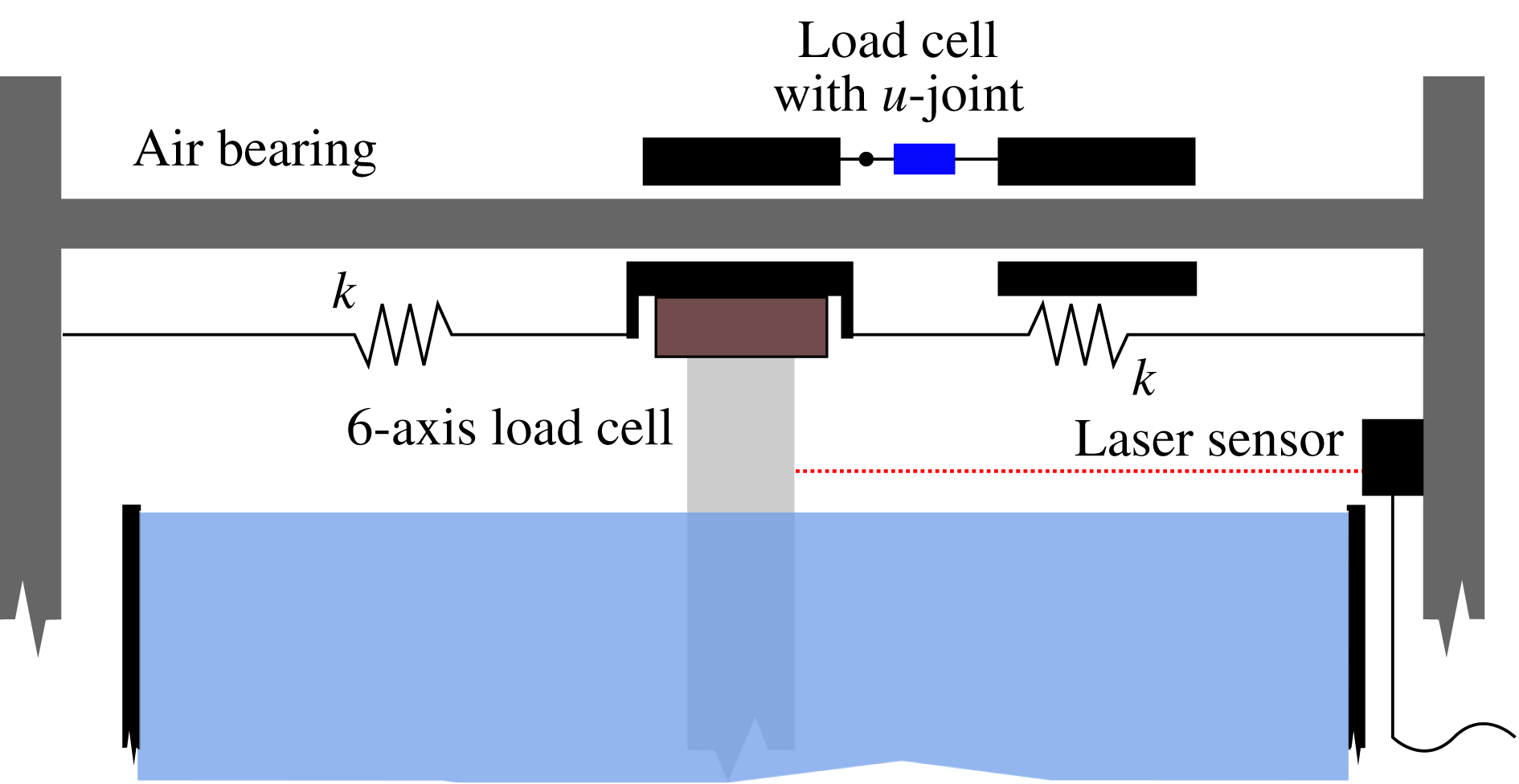One of the cylinders was held stationary with respect to the main structure whilst the other was able to oscillate with one degree of freedom thanks to a especially designed air-bearing system. The moving model had an end plate attached to its bottom end in order to prevent cylinder end effects there. Restoring forces in the free-to-move cylinder were provided by a set of springs with equivalent stiffness ( $k$ ) that connected the cylinder to the supporting structure. The moving cylinder hung from a one-degree-of-freedom air-bearing rig in which the only motions allowed were those in a direction perpendicular to the flow direction or cross-flow ( $y$ ). The experimental rig allowed the configuration of different centre-to-centre separations ( $S_{y}$ ) between the stationary and the moving cylinders. The separation is set with respect to the equilibrium position of the oscillating cylinder. Throughout the text, the term gap distance or separation distance are used indiscriminately to refer to the centre-to-centre separation resulting from the initial rest position, but note that the gap is in fact continuously varying as the vibrating cylinder moves depending on the imposed free-stream velocity. A Cartesian reference system is used in this work with its centre 0.25 m below the free surface (at the middle of the submerged part of the cylinder), with positive $x$ in the direction of the flow. The $z$ axis is coincident with the axis of the cylinder in its equilibrium position, with its positive direction pointing to the free water surface from below.

A non-intrusive laser-based displacement sensor was used to measure the motion of the cylinder in the cross-flow direction. For each experiment, the signal was sampled at 2 kHz for a period of 90 s, ensuring more than 90 oscillation cycles per run. The forces acting on the cylinder were also measured synchronously at the same sampling rate, by using a 6-axis load cell installed at its top end, connecting the model to the air-bearing carriage. The sensor allowed direct measurement of the in-line and transverse forces acting on the cylinder, and had a measurement range in these directions of $\pm 100$  N. Because the measured forces were of the order of $\pm 5$  N, therefore covering only 5 % of the full scale range of the sensor, alternative ways of obtaining the forces were used to validate and make the measurements redundant. In some specific cases, and for validation purposes only, a second completely independent precision uni-axial load cell (with a measurement range of $\pm 8.9$  N) was used to measure the transverse excitations. Both methods gave practically identical results. Transverse forces were computed using a third independent method based on the displacement data, and also showed excellent agreement. A detailed description of the force measurements is given in § 4.1. This redundancy also indirectly validated the case of the drag of forces presented in § 4.3, obtained by using a 6-axis load cell, being the only available method for measuring them.

Decay tests in air showed a very low damping coefficient ( $c$ ). If expressed as a ratio of the critical damping ( $\unicode[STIX]{x1D709}$ ), its value was 0.0054. The total structural mass of the system ( $m$ ), including the air-bearing carriage, load cell, cylinder model and the parts used to connect them all, yield a mass ratio ( $m^{\ast }=4m/\unicode[STIX]{x1D70C}\unicode[STIX]{x03C0}LD^{2}$ of 2.43, with $\unicode[STIX]{x1D70C}$ being the fluid density). The combined mass-damping parameter ( $m^{\ast }\unicode[STIX]{x1D709}$ ) ended up being as low as 0.013. The Reynolds number based on the cylinder model diameter ( $Re=UD/\unicode[STIX]{x1D708}$ , where $U$ and $\unicode[STIX]{x1D708}$ are respectively the free-stream velocity and the water kinematic viscosity) ranged from approximately $6000$ to $23\,000$ . The ratio between the free-stream velocity in the channel and the average velocity of the cylinder (based on its natural frequency in air $f_{o}$ ) is defined as the reduced velocity $U^{\ast }=U/f_{o}D$ , and ranged from slightly over 3 to more than 11. A schematic with a cross-sectional view of the models installed in the water and a cross-sectional view of the experimental layout appear in figure 1.

Once a certain centre-to-centre distance was fixed between the cylinders, experiments were conducted by changing the free-stream velocity in the channel. A total of six different separations $S_{y}/D=[2,2.5,3,3.5,4,5]$ were investigated and, for each one of them, $U^{\ast }$ was varied in small steps, yielding a data set consisting of more than 140 experiments. The lower limit in the spacing was set to $2D$ because tests with a separation of $1.5D$ showed contact between the models in most of the experiments in which the cylinder responded with large motions. For comparison and reference, experiments were also conducted with the isolated cylinder oscillating without wake interference.

Time-resolved digital particle image velocimetry (TR-DPIV) was used to investigate the flow around the cylinders in some specific cases of interest. Images were recorded at 500 fps using a CCD-sensor with 12-bit resolution, a pixel size of $10~\unicode[STIX]{x03BC}\text{m}$ and $1280\times 1024$ pixels, in combination with a lens with 20 mm fixed focal length. The flow was seeded using $20~\unicode[STIX]{x03BC}\text{m}$ neutrally buoyant polyamide particles and the illumination was generated using a continuous wave (CW) diode-pumped solid state (DPSS) green laser, able to deliver up to 5 W. This set-up allowed measurements of the velocity field in a planar $xy$ region of approximately $8\times 5$ diameters around the cylinder model, located at $z=0$ (at the middle of submerged part of the cylinder). Image preprocessing using in-house codes was performed in order to mask regions without particles in the flow and to identify in each DPIV snapshot the position of the cylinder model. After this initial preprocessing, a fast Fourier transform (FFT) cross-correlation algorithm (Willert & Gharib Reference Willert and Gharib1991) was applied to the preprocessed images, using an interrogation area of $32\times 32$ pixels with a 50 % area overlap. Spurious vectors produced by the cross-correlation scheme were thresholded and replaced by new values obtained from neighbouring interpolation.

Figure 1.

Experimental set-up. (a) Schematic view of the experimental set-up in the free surface water channel. (b) Cross-sectional schematic of the experimental arrangement.

Figure 2.

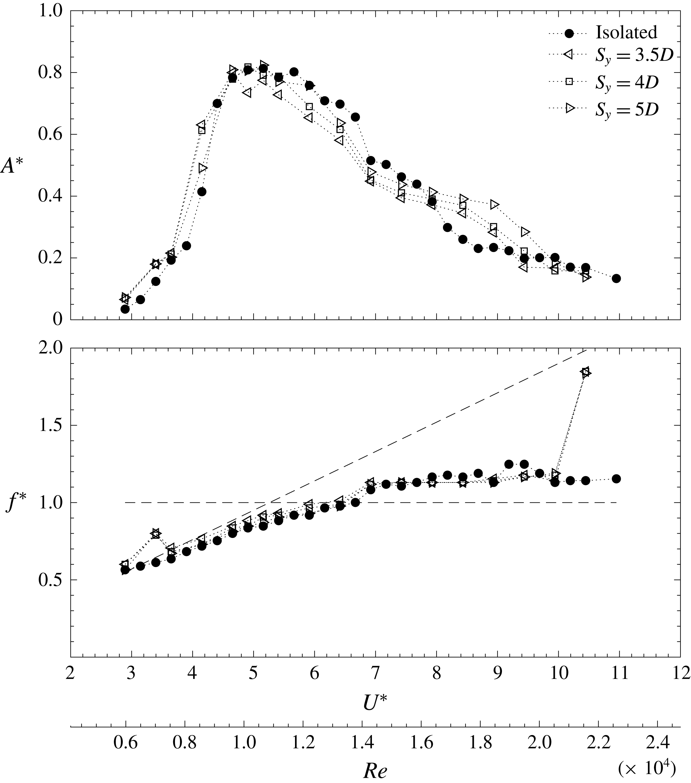
Dimensionless amplitude ( $A^{\ast }$ ) and frequency ( $f^{\ast }$ ) as a function of reduced velocity ( $U^{\ast }$ ) and Reynolds number ( $Re$ ), for the experiments conducted with gaps ( $S_{y}$ ) of $3.5D$ , $4D$ and $5D$ .

3 Dynamic response of the cylinder for different side-by-side separations

In this section the amplitude and frequency response of the elastically mounted cylinder is presented at all centre-to-centre separations investigated. In figures 2 and 3 the amplitude and frequency results obtained with the isolated cylinder appear with solid symbols for reference. The VIV amplitude response is characterised by the initial, upper and lower branches, as described in previous works with low mass-damping cylinders (Williamson & Govardhan Reference Williamson and Govardhan2004). Here the maximum amplitude achieved by the model was slightly more than $0.8D$ at reduced velocities around 5. The value presented in panel ( $a$ ) is the dimensionless amplitude $A^{\ast }$ that results from computing the mean of the values that envelope the time series of the displacement $y(t)$ , as in previous works such as Huera-Huarte & Bearman (Reference Huera-Huarte and Bearman2009), Huera-Huarte (Reference Huera-Huarte2017), Jiménez-González & Huera-Huarte (Reference Jiménez-González and Huera-Huarte2017). This value gives a very clear indication of the amplitude and is practically identical to $\sqrt{2}\widetilde{y}$ , with the tilde indicating the standard deviation of the time series of the displacement. Furthermore, as expected, the isolated cylinder oscillation frequency followed the Strouhal law in the initial branch when the motions were very small and the vortex shedding process dominated the dynamics. The Strouhal frequency appears represented in the plots with an inclined dashed line, with a slope of 0.18. As the reduced velocity is increased to the upper branch, with the response locked in and the cylinder undergoing large motions, the slope of the frequency response curve is changed, staying at values near the natural frequency of the system (horizontal dashed line in the figure). The same happens in the lower branch, where the fluid–structure interaction process still dominates the response, but with values away the natural frequency of the system. If $U^{\ast }$ could be further increased, surpassing the maximum reduced velocities achievable in these experiments, the cylinder would again tend to follow the frequencies imposed by the shedding process, undergoing very small motions. In the lower plots of figures 2 and 3, the frequency is shown in dimensionless form ( $f^{\ast }$ ) as the ratio of the dominant frequency in the experiment to the natural frequency of the system in air ( $f_{0}$ ).

Figure 3.

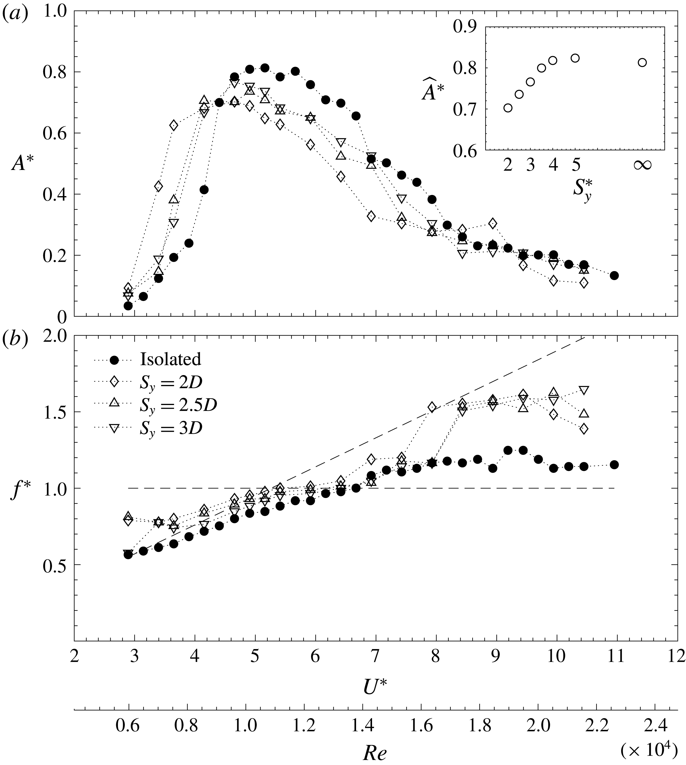
Dimensionless amplitude ( $A^{\ast }$ ) and frequency ( $f^{\ast }$ ), as a function of reduced velocity ( $U^{\ast }$ ) and Reynolds number ( $Re$ ), for the experiments conducted with gaps ( $S_{y}$ ) of $2D$ , $2.5D$ , $3D$ . The inset plot shows the maximum dimensionless response ( $\widehat{A}^{\ast }$ ) attained by the cylinder as a function of separation distance ( $S_{y}^{\ast }$ ).

In figure 2, the results for the experiments conducted with gaps of $3.5D$ , $4D$ and $5D$ are compiled together with those from the isolated system. Although some differences in the displacements can be observed, the levels of amplitude and the trends exhibited by all four configurations are very similar. As commented upon before for the isolated cylinder case, in all four sets of experiments the initial, upper and lower branches can be identified as in the isolated case. The same happens with the frequency response, which is very similar at all the separations that appear in the figure. Nevertheless, there is a jump in the frequency points with $U^{\ast }>10$ to the shedding frequency values, which in the isolated cylinder case did not occur before reaching the maximum achievable velocities in the channel. Another minor difference in the frequency response took place at the smallest reduced velocities, where the frequency points in all the cases with wake interference showed a small kink in the data. These results clearly indicate that the effect that the stationary cylinder had on the VIV response of the oscillating cylinder was very limited at these large centre-to-centre separations.

If the gap between the cylinders is reduced, the response of the oscillating cylinder is highly altered, as can be seen in figure 3. The gap flow now is crucial in the response of the system, as differences are more evident. Plots for the cases with separations of $2D$ , $2.5D$ and $3D$ appear together with the isolated case. In the figure, it is also clear how the maximum attained amplitudes decreased with decreasing separations. The inset plot in figure 3 shows the maximum amplitude ( $\widehat{A}^{\ast }$ ) for each separation investigated and how, when the imposed separations are $4D$ or more, the amplitude values remain very similar to those for the isolated cylinder. It also shows how the amplitude decreases monotonically to values near 70 % of the cylinder diameter as the gap is reduced. In general, the response curves in figure 3 have similar trends – all exhibiting initial, upper and lower branches, but with smaller amplitudes. Moreover, the smaller the separation, the smaller the reduced velocity at which the maximum takes place. There is a shift of the curves to lower values of reduced velocity, so although the cylinder exhibits the same response branches, they start at smaller reduced velocity values, finishing before. For comparison, it is remarkable how, when the separation was set to $2D$ , the VIV amplitude measured at a reduced velocity of 3.5 was more than $0.4D$ , whilst in the isolated cylinder case was around four times less. The amplitudes tend to similar levels, only for values of reduced velocity larger than 8.5. All these effects were only seen in the cases presented in figure 2 with larger gaps. By comparing the isolated cylinder data with the cases with interference, it is clear that the shift of the lock-in region to smaller $U^{\ast }$ can be attributed to the effect of the proximity of the stationary cylinder. This result is in agreement with the numerical simulations carried out by Liu & Jaiman (Reference Liu and Jaiman2016), where the same shift of the lock-in region was observed. In their case, however, the response region was considerably narrower (more than a 40 %). This narrowing effect observed by Liu & Jaiman (Reference Liu and Jaiman2016) could be caused by differences, not only in $Re$ , but also in the mass-damping parameter, one order of magnitude higher in their simulations, as it is well known that the extent of the lock-in region is highly dependent on the combined mass-damping parameter and the Reynolds number. Narrow lock-in regions of VIV response have been shown in cylinders with either high mass ratio (Williamson & Govardhan Reference Williamson and Govardhan2004) or at low $Re$ (Anagnostopoulos & Bearman Reference Anagnostopoulos and Bearman1992).

Figure 3( $b$ ) shows the effects of the stationary cylinder on the frequency response of the model. In general, as the gap is reduced, the dimensionless dominant frequencies in the response become larger. From reduced velocities of approximately 3.5 up to 8, the curves follow the same trend as in the case of the isolated cylinder, but at higher $f^{\ast }$ values. Under 4, the interference causes the frequencies to stay at higher values than those observed in the isolated case, not following the Strouhal law, but staying at values between the natural frequency of the system and the shedding frequency. This effect barely occurred when the separation distances were larger than $3D$ (figure 2), showing only the small kink in the data described before. For reduced velocities higher than 8, the frequencies of the cylinder with interference are closer to the expected shedding frequencies, with values of about 1.5 times the natural frequency. The planar velocimetry data presented in § 5 will help to describe the physics behind this frequency enhancement due to the proximity interference.

Figure 4.

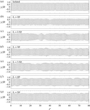
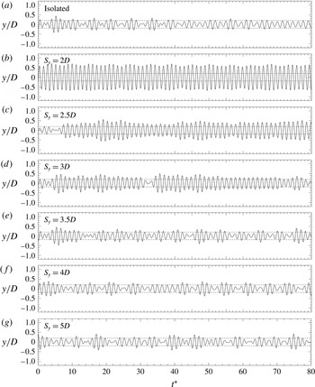
Time series of the dimensionless VIV amplitudes for experiments conducted with $U^{\ast }\approx$ 5 in all configurations. For easier comparison, horizontal dashed lines are used to indicate the amplitude of the isolated cylinder case in all the plots.

Figure 5.

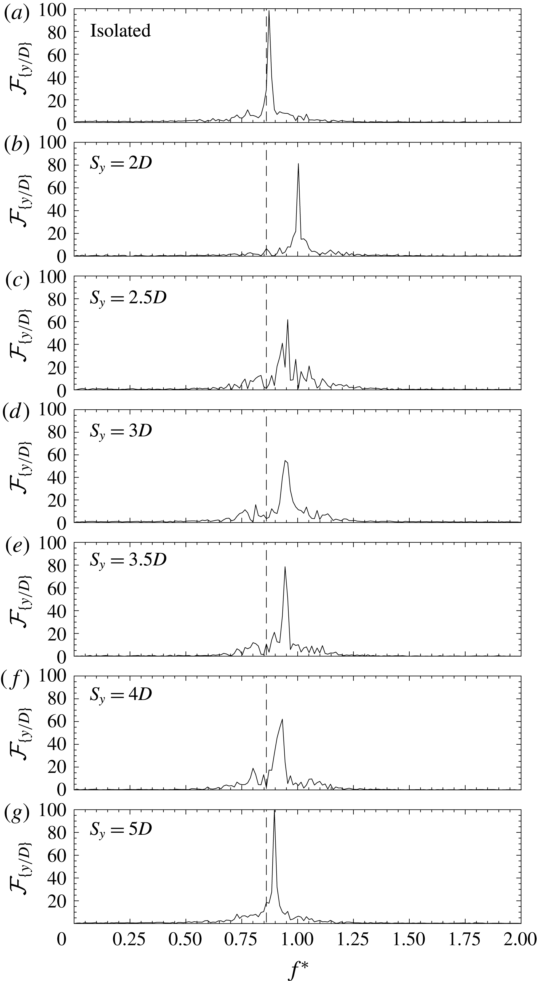
Spectra of the VIV amplitudes for experiments conducted with $U^{\ast }\approx$ 5 in all configurations. For easier comparison, vertical dashed lines are used to indicate the dimensionless dominant frequency of the isolated cylinder case in all the plots.

The experiments conducted at $U^{\ast }$ near lock-in conditions in the upper branch showed amplitudes that were mostly harmonic without modulation in all cases. Figure 4 clearly depicts this situation, as well as the fact that amplitudes differed, when compared to the isolated case, only at the smallest separations, as shown previously in figures 2 and 3. In the plots, the time series of the dimensionless amplitude ( $y^{\ast }=y/D$ ) for all configurations appear as a function of the dimensionless time $t^{\ast }=tf_{o}$ . For easier comparison, horizontal dashed lines are used in all the plots to indicate the amplitude of the isolated cylinder case. A very weak amplitude modulation can be observed only when gaps were smaller than $3.5D$ . This is not surprising, because in the lock-in range the correlation lengths are known to be high, as the large-amplitude motions and the natural frequency of the system take over the vortex shedding instability mechanism (Bearman Reference Bearman1984). The spectra in figure 5 show how, as the gap is reduced, the dominant frequency tends to increase, earlier approaching the natural frequency of the system. In figure 4, all the spectral amplitudes ( ${\mathcal{F}}_{\{y^{\ast }\}}$ ) are normalised as a percentage of the maximum between all of them. For comparison, the vertical dashed lines in the plots indicate the dominant frequency of the isolated cylinder case.

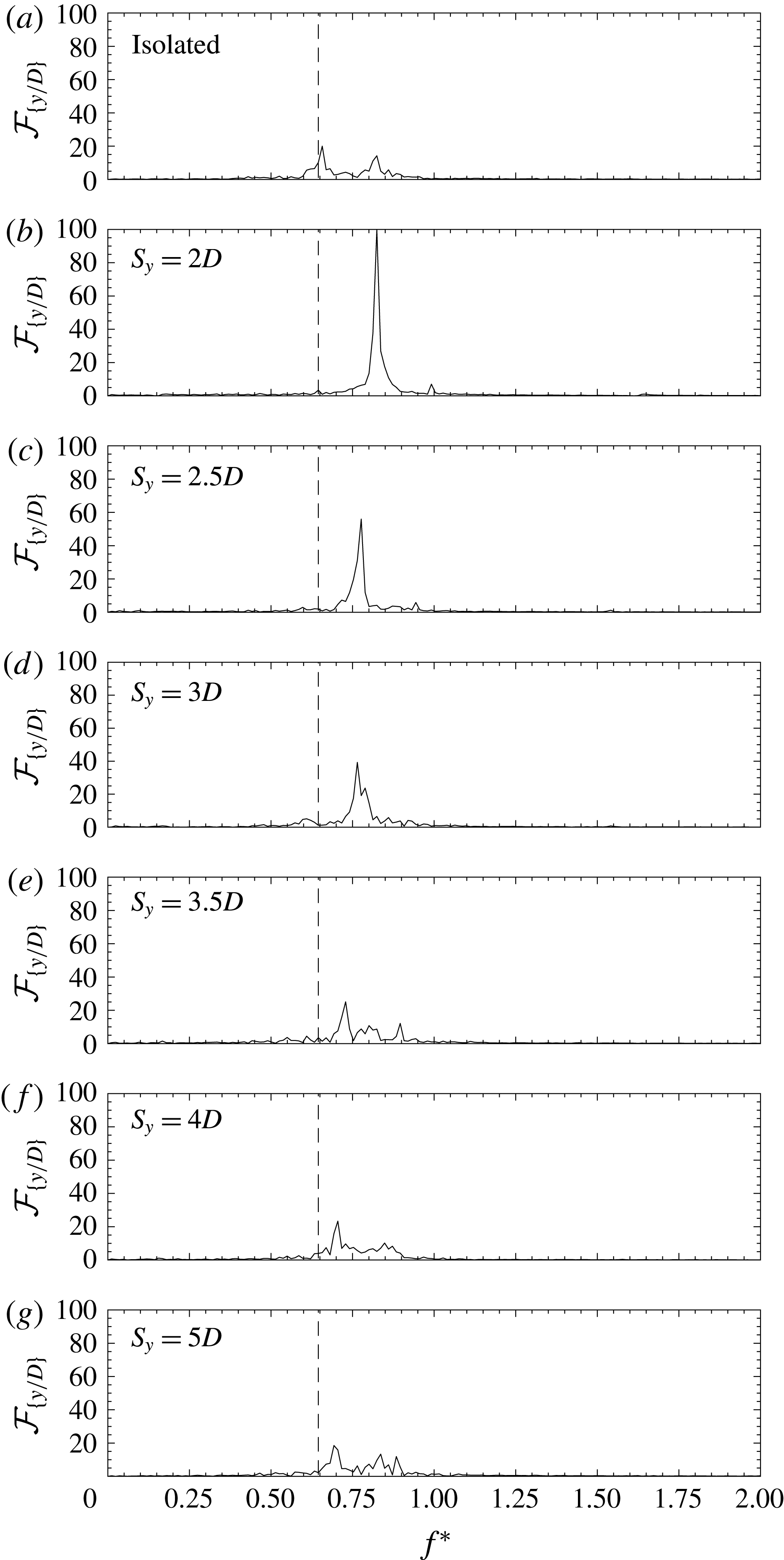
When the reduced velocity was set to values near 3.5, outside the expected lock-in range, the amplitudes were highly modulated, as can be seen in figure 6. For an isolated cylinder, in this regime, the spanwise correlation of vorticity tends to be small. This leads to wider-band spectra and parameters that become highly variable along the length of the cylinders (Bearman Reference Bearman1984). The modifications introduced in the response by the wake of the near-stationary cylinder for gaps larger than $3D$ were very small. Notwithstanding, for smaller gaps the differences are obvious; in fact, when the separation is $2D$ the amplitude modulation was highly reduced. The spectra in figure 7 show harmonic motions with a narrow banded response only when the gaps are the smallest.

Figure 6.

Time series of the dimensionless VIV amplitudes for experiments conducted with $U^{\ast }\approx$ 3.5 in all configurations. For easier comparison, horizontal dashed lines are used to indicate the amplitude of the isolated cylinder case in all the plots.

Figure 7.

Spectra of the VIV amplitudes for experiments conducted with $U^{\ast }\approx 3.5$ in all configurations. For easier comparison, vertical dashed lines are used to indicate the dimensionless dominant frequency of the isolated cylinder case in all the plots.

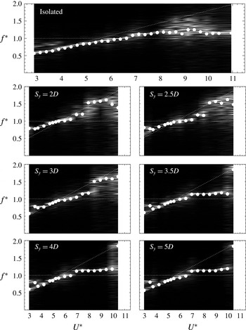
The frequency content of the response can be further seen in the form of spectrograms in figure 8. The frequency response appears as a function of reduced velocity for each data set studied. White dots in the plots are for the dominant frequencies, as they appeared in figures 2 and 3. The horizontal dashed line refers to the value $f^{\ast }=1$ where the response frequency is equal to the natural frequency of the system. The inclined line with a slope of 0.18 indicates the expected shedding frequency. The spectrogram of the isolated cylinder clearly shows wider spectra at the smallest reduced velocities ( $U^{\ast }\leqslant 4$ ), which can be associated, as commented upon before, to the small amplitudes in the initial branch of response and to a poorly spanwise correlated flow, as suggested by Bearman (Reference Bearman1984). This is a common feature in all the spectrograms with large centre-to-centre separations ( $S_{y}>3D$ ). However, for small separations the plots show how frequencies tend to depart from the inclined line to the horizontal line, i.e. from the vortex shedding frequency to the natural frequency of the system, indicating a resonant condition that does not take place in the isolated case. This will be further studied in the following section, in relation to the excitation acting on the cylinder.

Figure 8.

Spectrograms showing the frequency response as a function of reduced velocity for each data set. White dots are for the dominant frequencies as they appeared in figures 2 and 3. The horizontal dashed line indicates $f^{\ast }=1$ and the inclined line has a slope of 0.18, indicating the expected shedding frequency.

4 Hydrodynamic forces acting on the cylinder

4.1 Computation of the transverse forces

As introduced in figure 1, in addition to the dynamic response of the cylinder, fluid excitation in the transverse direction ( $F_{y}$ ) was also measured. A very straightforward method for computing the transverse forces uses the measured displacements and the one-degree-of-freedom mathematical model of the system given by

(4.1) $$\begin{eqnarray}m\ddot{y} +c{\dot{y}}+ky=F_{y},\end{eqnarray}$$

where $y$ is the time-dependent displacement of the cylinder and the dots indicate time differentiation. After summing the terms, the force is presented in dimensionless form as the transverse force coefficient,

(4.2) $$\begin{eqnarray}C_{y}=\frac{F_{y}}{\frac{1}{2}\unicode[STIX]{x1D70C}U^{2}DL}.\end{eqnarray}$$

Several authors (Brankovic Reference Brankovic2004; Seyed-Aghazadeh, Carlson & Modarres-Sadeghi Reference Seyed-Aghazadeh, Carlson and Modarres-Sadeghi2015; Seyed-aghazadeh & Carlson Reference Seyed-aghazadeh and Carlson2017) have successfully calculated transverse forces using the same concept. Although transverse forces were measured using a 6-axis load cell, as described in figure 1, all the forces presented in § 4.2 have been computed as described above, using (4.1). This was done to ensure the maximum possible accuracy in the results, because measured forces were of the order of 5 % of the measurement range of the multi-axis load cell. Results also include the phase difference between displacement and excitation ( $\unicode[STIX]{x1D719}$ ). With the time series of the force available, phases have been computed using the Hilbert transform and the analytical signal concept (Panter Reference Panter1965; Rosenblum, Pikovsky & Kurths Reference Rosenblum, Pikovsky, Kurths, Schimansky-Geier and Pöschel1997) applied previously to VIV problems (Khalak & Williamson Reference Khalak and Williamson1999; Huera-Huarte & Bearman Reference Huera-Huarte and Bearman2009).

For validation purposes, the forces were also obtained using a third independent method that consisted of measuring transverse forces directly with a uni-axial load cell arrangement. This was done only in certain experiments, again for validation purposes. A second frictionless air-bearing carriage was added to the main air-bearing beam, and a precision tension/compression load cell (measurement range $\pm 8.9$  N with 0.01 % accuracy) was used to connect the two carriages, allowing direct measurement of the transverse force. This arrangement was not kept during the whole set of experiments because the modifications it required considerably increased the mass of the moving system, resulting in a mass ratio 45 % higher. One of the design requirements of the experiments was to keep the mass-damping of the system as low as possible, which is why, after the validation exercise, the force measuring set-up based on the uni-axial load cell was not used any more. For these validation experiments, the force output given by the uni-axial sensor was sampled synchronously with the rest of the signals, at 2 kHz. The connection between the carriages and the load cell was made through universal joints to avoid the transmission of moments in the event of small mounting misalignments. A schematic of the modified set-up appears in figure 9.

Figure 9.

Schematic view of the transverse force measurement arrangement.

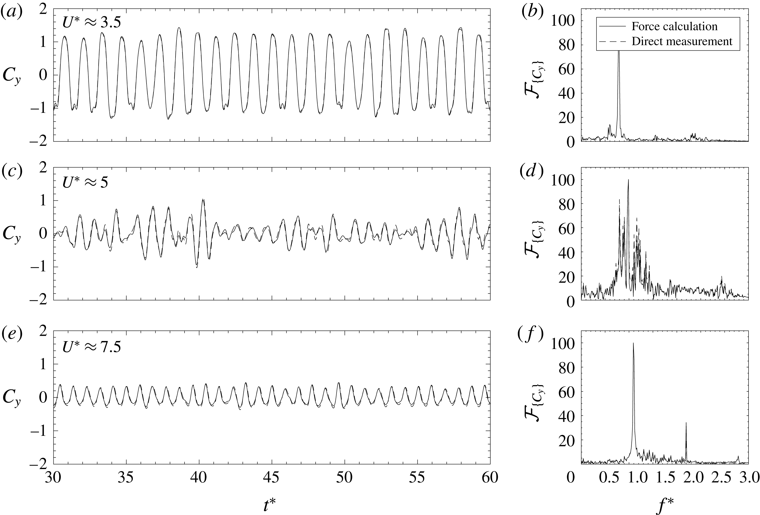
Results with the comparison of the direct measurements and the force calculations based on (4.1) appear in figure 10, for three isolated cylinder cases with different reduced velocities of approximately 3.5, 5 and 7.5, covering different regions of the response curve. Panels (a,c) of the figure show the time series of transverse force coefficients ( $C_{y}(t)$ ) and panels (b,d) their corresponding spectra ( ${\mathcal{F}}_{\{C_{y}\}}$ ). Spectra are scaled to 100 for representation purposes. In the figure, solid lines indicate that the results were derived from (4.1) and dashed lines are used for the results obtained by direct measurement with the uni-axial load cell. For all reduced velocities tested, the results showed an extremely good agreement, validating the methodology here described, and indicating that the load cell arrangement with the associated increase in mass ratio could be avoided.

Figure 10.

Time series of the transverse force coefficient and spectra for the isolated cylinder at reduced velocities of approximately 3.5, 5 and 7.5. Each plot shows the coefficients and the spectra obtained by the methodology described by (4.1) (solid line) and by direct force measurements (dashed lines).

4.2 Effects of side-by-side separation on transverse forces

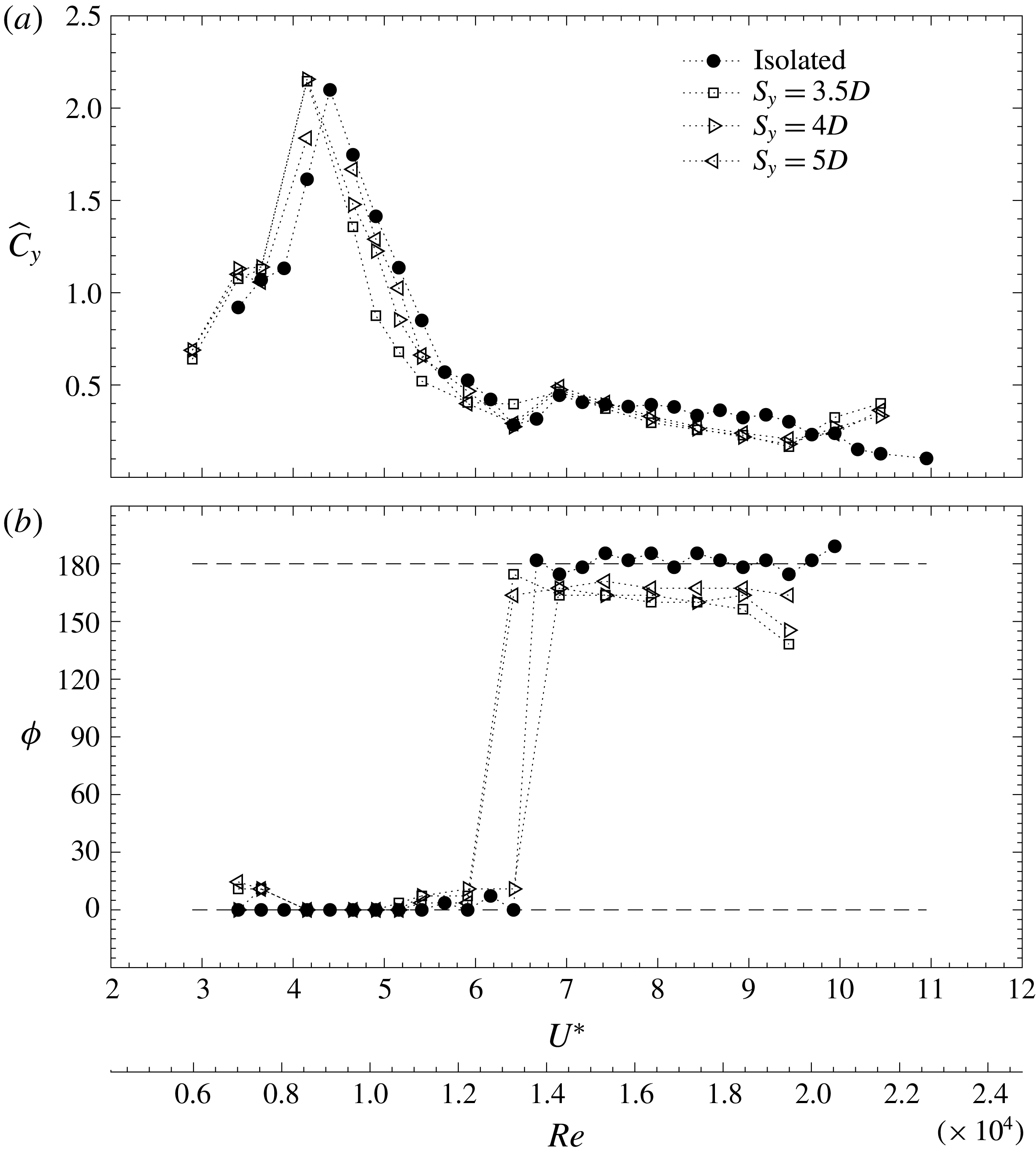
The transverse force coefficients ( $\widehat{C}_{y}=\sqrt{2}\widetilde{C}_{y}$ ), computed as detailed in the previous section, are presented in figure 11( $a$ ) for the experiments conducted with the largest separations. $\widetilde{C}_{y}$ is the standard deviation of the time series of the lift coefficient. In figure 11( $b$ ) the phase difference between the displacement and the excitation $\unicode[STIX]{x1D719}$ is also shown. As happened with the dynamic response, when separations are large, forces tend to be similar to those of the isolated case. In the first part of the initial branch the excitation ramps up very quickly to its maximum as in a resonance condition, and then very quickly drops to its minimum at the end of the upper branch. In the lower branch, the value of the coefficient remains at very low levels near the minimum. The excitation is in phase with the displacement in the initial and upper branches. At the end of the upper branch, the phase jumps $180^{\circ }$ , indicating that excitation and motion are out of phase.

Figure 11.

Dimensionless transverse force coefficient ( $\widehat{C}_{y}$ ) and phase ( $\unicode[STIX]{x1D719}$ ) as a function of reduced velocity ( $U^{\ast }$ ) and Reynolds number ( $Re$ ), for the experiments conducted with gaps ( $S_{y}$ ) of $3.5D$ , $4D$ and $5D$ . Horizontal dashed lines in ( $b$ ) indicate in-phase ( $0^{\circ }$ ) and out-of-phase ( $180^{\circ }$ ) situations between motion and excitation.

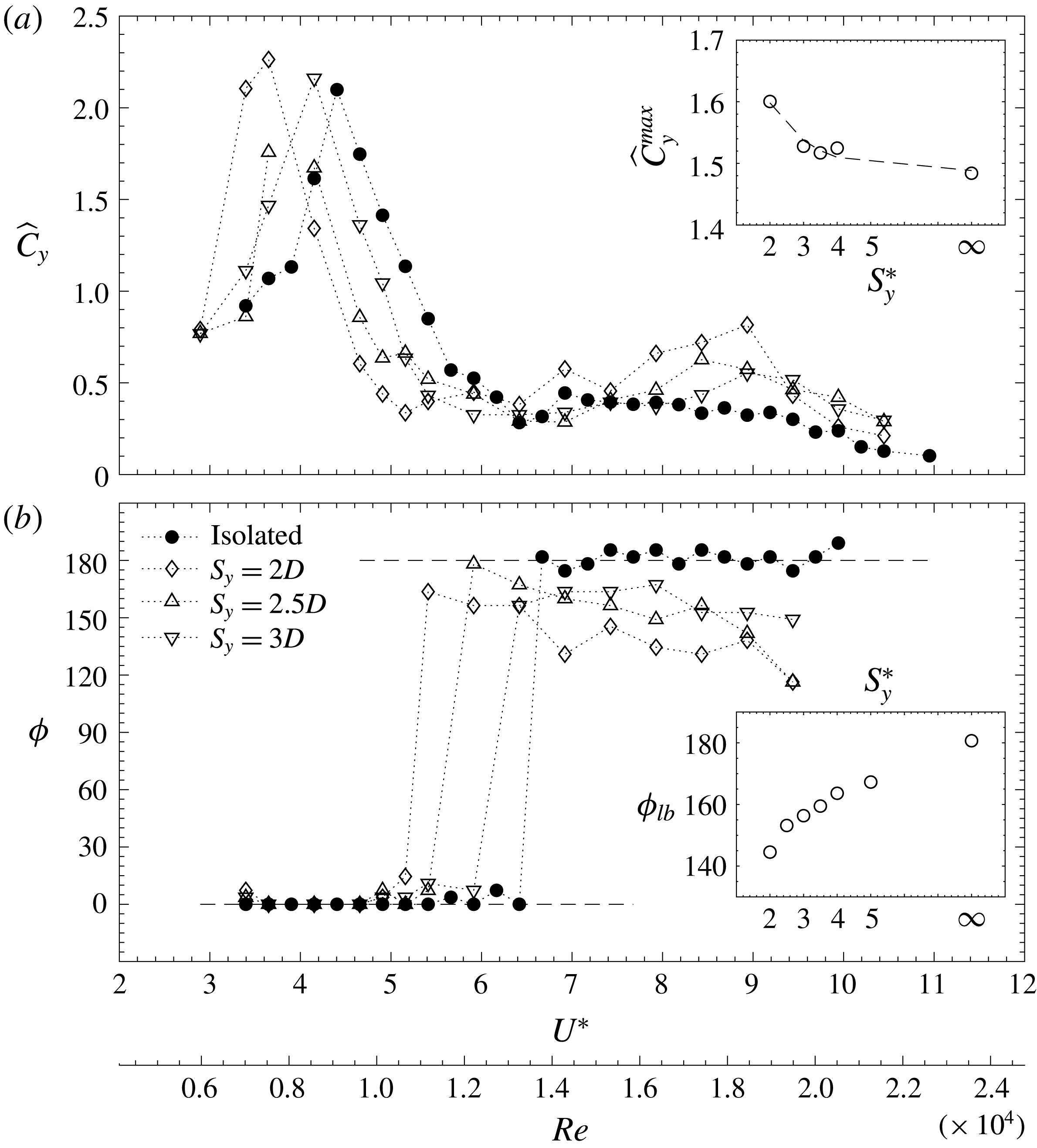
When the interference takes place at the smaller separations investigated, the excitation curves and phase differences change remarkably, as happened with the dynamic response. In figure 12, the transverse coefficient curves appear to shift to the left in the reduced velocity axis, as happened with the dynamic response in figures 2 and 3. The trend depicted by the curves is the same as in the isolated case, with a sudden increase of the transverse force up to their maximum, followed by a sudden drop to their minima. In the isolated case, the end of the upper branch took place at a reduced velocity slightly under 7, whilst in the case with the smaller gap between the models, it took place at approximately 5. The peak values ( $\widehat{C}_{y}^{max}$ ) in the curves become larger, as the interference is stronger at the smaller separations. An inset plot shows an exponential decay of the transverse force peak with increasing separation distance, to values near 1.5 for the isolated case. Note that the plot does not include the maxima of cases with separations of $2.5D$ and $5D$ , because of the resolution in the reduced velocity axis. The free surface water channel (FSWC) is a large facility, and has limitations in how small the changes in the free stream can be from one point to another, so when conducting the experiments, the peaks for these two cases fell in between one of these velocity jumps.

The displacement of the force coefficient curves to smaller reduced velocities is also very evident by looking at the jump in phase ( $\unicode[STIX]{x1D719}$ ) associated with the end of the upper branch in figure 12( $b$ ). In fact, the jump, which has a value of $180^{\circ }$ (motion and forcing are out of phase) in the case of the isolated cylinder, becomes smaller as the gap between the cylinders is reduced. In the case of a separation of $2D$ , the phase difference in the lower branch stays in the range from $120^{\circ }$ to $150^{\circ }$ . The inset plot in figure 12 depicts the mean value of the phase difference in the lower branch ( $\unicode[STIX]{x1D719}_{lb}$ ) and how it grows monotonically up to the out-of-phase situation measured with the isolated cylinder. Recent numerical results by Liu & Jaiman (Reference Liu and Jaiman2018) have also shown this phenomena, with smaller gap separations causing the phase angle between excitation and response to be reduced to values near $90^{\circ }$ .

Figure 12.

Dimensionless transverse force coefficient ( $\widehat{C}_{y}$ ) and phase ( $\unicode[STIX]{x1D719}$ ) as a function of reduced velocity ( $U^{\ast }$ ) and Reynolds number ( $Re$ ), for the experiments conducted with gaps ( $S_{y}$ ) of $2D$ , $2.5D$ and $3D$ . Horizontal dashed lines in ( $b$ ) indicate in-phase ( $0^{\circ }$ ) and out-of-phase ( $180^{\circ }$ ) situations between motion and excitation. The inset plot shows the phase differences in the lower branch ( $\unicode[STIX]{x1D719}_{lb}$ ), after the phase jump, as a function of centre-to-centre separation ( $S_{y}^{\ast }$ ).

At the smallest separations, despite the fact that, in the initial branch, displacement and excitation are in phase, and the lift coefficients are larger, amplitudes are smaller. The enhanced forcing is accompanied by an increase in the oscillating frequencies (see figures 2 and 3), which in turn is related to the amplitude of VIV motion and to the limiting effect caused by the proximity of the stationary cylinder due to the existence of the gap flow. Other authors (Liu & Jaiman Reference Liu and Jaiman2016) have attributed this fact to a change in the location of the stagnation points caused by the gap flow interaction. Mathematical models for VIV include fluid forcing terms in which the loads are not only time dependent but amplitude and frequency dependent. An excellent review of these advanced forced models and of those based on the use of oscillator equations appears in Païdoussis et al. (Reference Païdoussis, Price and De Langre2010). Despite the existence of these more elaborate models of fluid forcing, it is common to describe the VIV loading term that appears in the one-degree-of-freedom model presented in (4.1) as a harmonic function of the form $F_{y}(t)=\widehat{F}_{y}\sin (2\unicode[STIX]{x03C0}ft+\unicode[STIX]{x1D719})$ . These models proved very useful in order to understand the crucial role of the phase between excitation and displacement on the dynamic response of the system. From the linear theory of vibrations it is easy to derive an expression for the amplitude in the system,

(4.3) $$\begin{eqnarray}A^{\ast }=\frac{1}{4\unicode[STIX]{x03C0}^{3}}\frac{U^{\ast ^{2}}}{m^{\ast }\unicode[STIX]{x1D709}f^{\ast }}\widehat{C}_{y}\sin (\unicode[STIX]{x1D719}),\end{eqnarray}$$

which indicates that the amplitude of the system is proportional to the part of the force in phase with velocity, and inversely proportional to the responding frequency. With increased frequencies, reductions of amplitude are expected, as observed in the experiments presented here.

The shift of the lock-in region to smaller reduced velocities as a consequence of small centre-to-centre separations, and the observation of very large amplitudes with responding frequencies departing from that of shedding (figures 3 and 8), and being characterised by narrow-banded spectra, can be linked to the forcing presented here. In fact that observation can be explained by the large excitations in phase with the motion presented in figure 12, which suggest that, when the separations are small, the forcing is highly correlated along the length of the model, because of the effect of the gap flow. The gap flow triggers, at earlier reduced velocities, the highly correlated flow that takes place in the upper branch of the response of an isolated cylinder at larger $U^{\ast }$ . This effect has also been observed in the numerical simulations of Liu & Jaiman (Reference Liu and Jaiman2018). The authors obtained the three-dimensional structure of the wake at moderate $Re$ , observing a two-dimensional recovery of the wake at small reduced velocities. The gap flow in the side-by-side arrangement forces the wake to be highly correlated if compared to that of an isolated cylinder at the same $U^{\ast }$ and $Re$ .

4.3 Effects of side-by-side separation on in-line forces

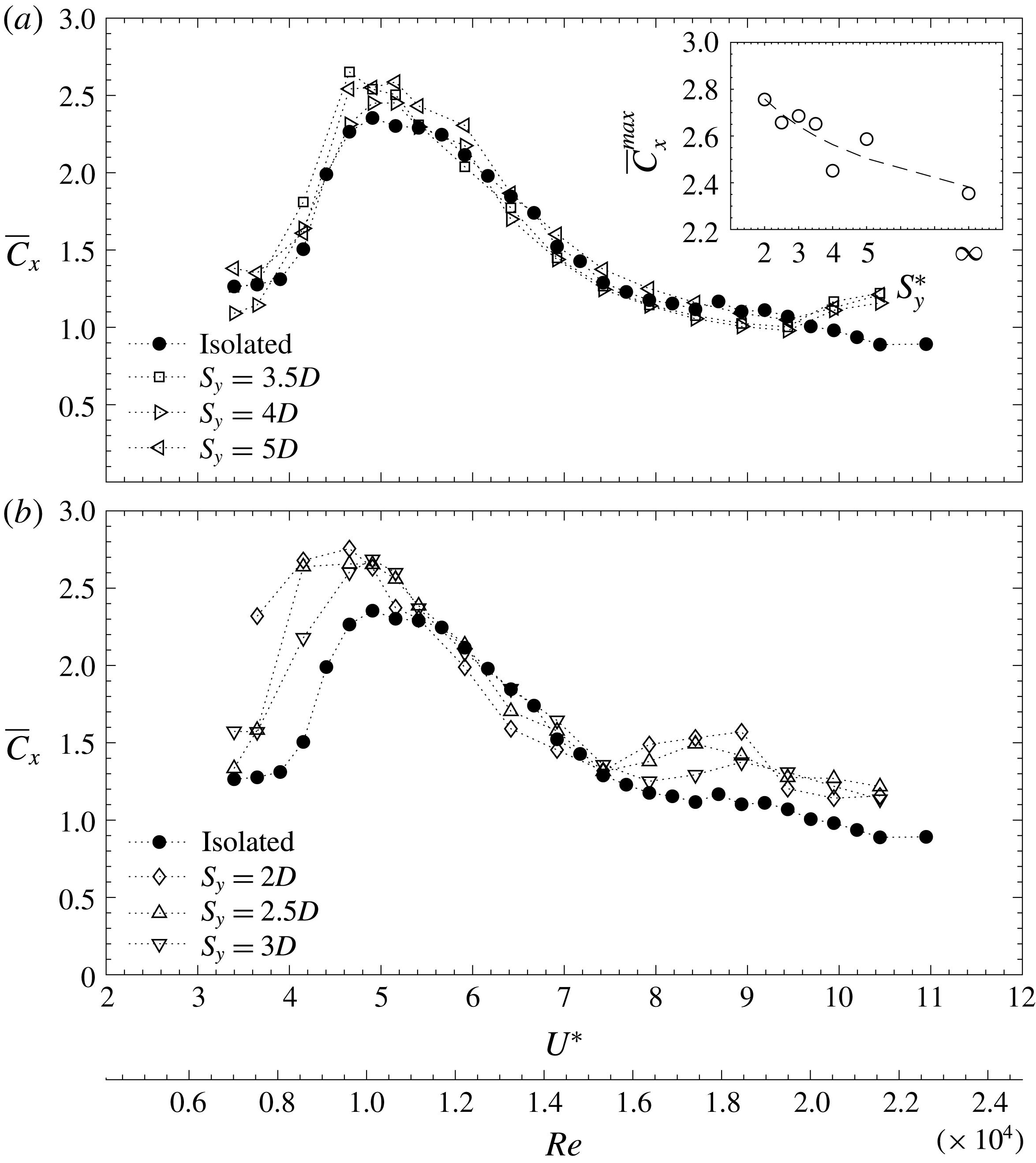
The time-averaged drag coefficients ( $\overline{C}_{x}$ ), measured using the multi-axis load cell arrangement described in figure 1, appear in figure 13. The coefficients result from expressing in dimensionless form the time-averaged in-line force ( $\overline{F}_{x}$ ),

(4.4) $$\begin{eqnarray}\overline{C}_{x}=\frac{\overline{F}_{x}}{\frac{1}{2}\unicode[STIX]{x1D70C}U^{2}DL}.\end{eqnarray}$$

At the largest centre-to-centre separations depicted in figure 13( $a$ ), forces clearly follow the same trend as that exhibited by an isolated cylinder. VIV drag coefficients remain at values near those of stationary cylinders at the same value of $Re$ , outside the lock-in region. In the initial branch, they grow monotonically with amplitude up to their highest values in the upper branch, and start descending again with the amplitude. Inside the lock-in region, coefficients are slightly larger in the cases with wake interference, reaching values up to 2.5.

Figure 13.

Dimensionless in-line force coefficient ( $\overline{C}_{x}$ ) as a function of reduced velocity ( $U^{\ast }$ ) and Reynolds number ( $Re$ ), for the experiments conducted with all the gaps studied.

Figure 14.

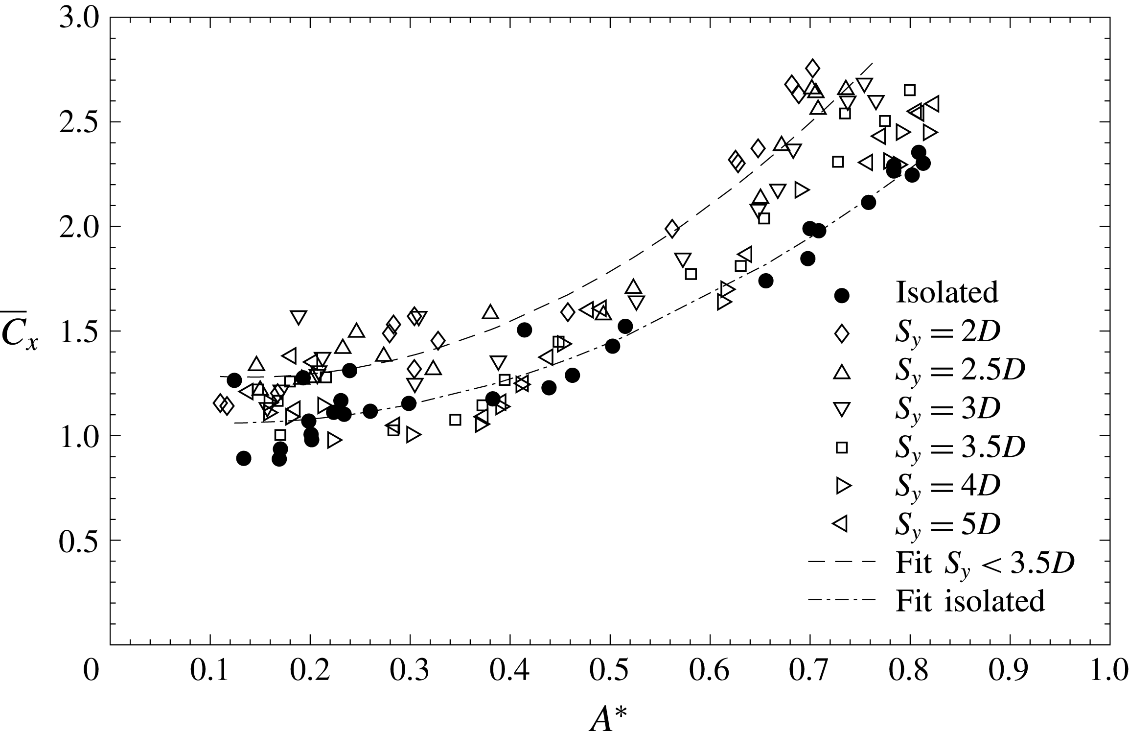
Dimensionless in-line force coefficient ( $\overline{C}_{x}$ ) as a function of dimensionless amplitude ( $A^{\ast }$ ) for all the experiments conducted. A quadratic fit is shown as a dashed line.

As happened with the response and the transverse excitation, the mean drag values are highly conditioned by the wake of the stationary cylinder when the separation distances are small (figure 13 $b$ ). At reduced velocities near 5, force coefficients are more than 2.5 and, in the case of separation distances of $2D$ and 2. $5D$ , these high values extend to reduced velocities of 4 and under, where the isolated cylinder exhibits coefficients of approximately 1.2. This is related to the shift of the response region commented upon in § 3, which is very clear for the two smaller separations. The inset plot in figure 13( $a$ ) shows how the maximum of the mean drag coefficient decreases monotonically with separation distance. For reduced velocities more than 8, the drag coefficient curves with interference deviate with respect to that of the isolated cylinder. This deviation was not observed in the amplitudes but appears in the frequencies, as can be seen in figure 3. The frequencies in the desynchronisation region jumped to the ones imposed by the shedding at a reduced velocity of approximately 8.

The fact that the in-line forces are highly conditioned by the displacements can be easily seen in figure 14, where force coefficients are plotted against dimensionless amplitudes. A fit for the isolated cylinder data points, using equation $\overline{C}_{x}=2.6A^{\ast ^{2}}-0.6A^{\ast }+1.1$ , has been included in the plot as a dashed-dot line, indicating a quadratic trend of the data, and therefore a drag amplification phenomena. If the fit is computed for the cases with the strongest interference, i.e. for $S_{y}<3.5D$ , it moves upwards, indicating the same trend with considerably higher force coefficients. The equation $\overline{C}_{x}=3.43A^{\ast ^{2}}-0.97A^{\ast }+1.27$ is included in the plot as a dashed line. This type of drag magnification with displacement has been reported previously not only in one-degree-of-freedom systems, but also in the case of vortex-induced vibrations of flexible cylinders (Chaplin et al. Reference Chaplin, Bearman, Huera-Huarte and Pattenden2005; Huera-Huarte & Bearman Reference Huera-Huarte and Bearman2009).

5 The wake of the system as a function of the side-by-side separation

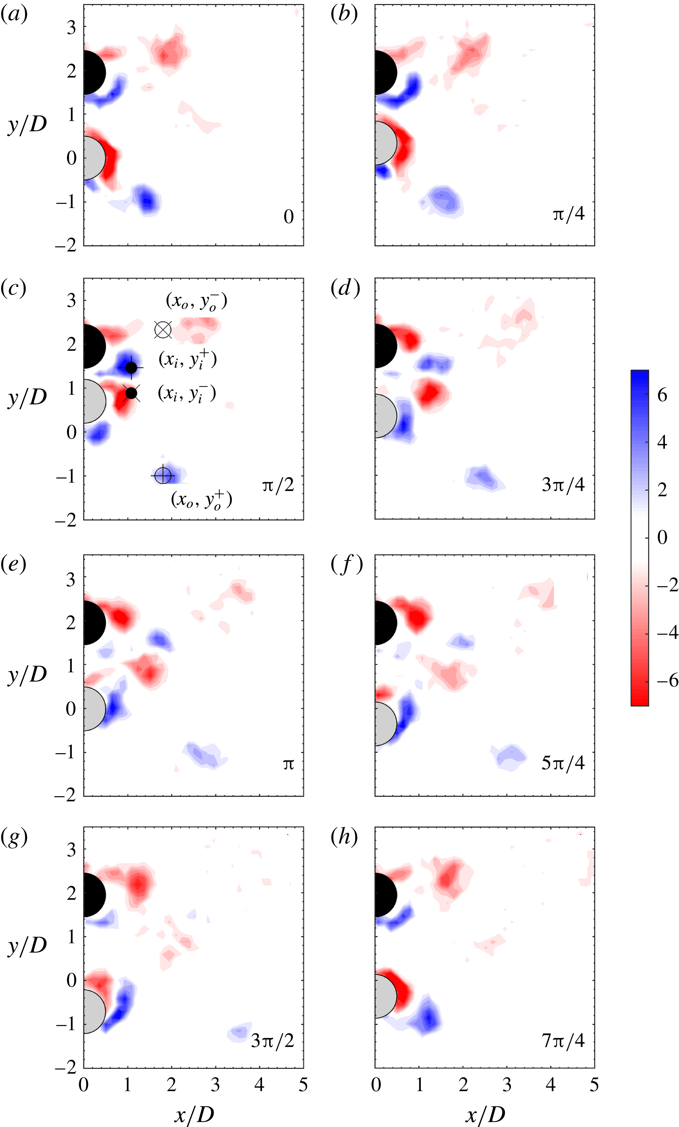
In some specific cases, the flow field in the wake of the models was obtained after DPIV measurements in order to help in elucidating the causes for the response and excitation dynamics described in the above sections. Results are presented in the form of vorticity or velocity fields. In all these figures the vorticity $\unicode[STIX]{x1D714}^{\ast }$ appears in the dimensionless form $\unicode[STIX]{x1D714}D/U$ and is phase averaged at eight positions (0, $\unicode[STIX]{x03C0}/4$ , $\unicode[STIX]{x03C0}/2$ , $3\unicode[STIX]{x03C0}/4$ , $\unicode[STIX]{x03C0}$ , $5\unicode[STIX]{x03C0}/4$ , $3\unicode[STIX]{x03C0}/2$ and $7\unicode[STIX]{x03C0}/4$ ) of an oscillation cycle. Velocity fields also appear in the dimensionless form and are result of time averaging the magnitude of velocity, as in $U^{-1}\sqrt{v_{x}^{2}+v_{y}^{2}}$ , where $v$ is used for the velocity in the $x$ or $y$ directions. The stationary cylinder appears in the figures in black and the elastically mounted cylinder appears in light grey for spatial reference.

Figure 15.

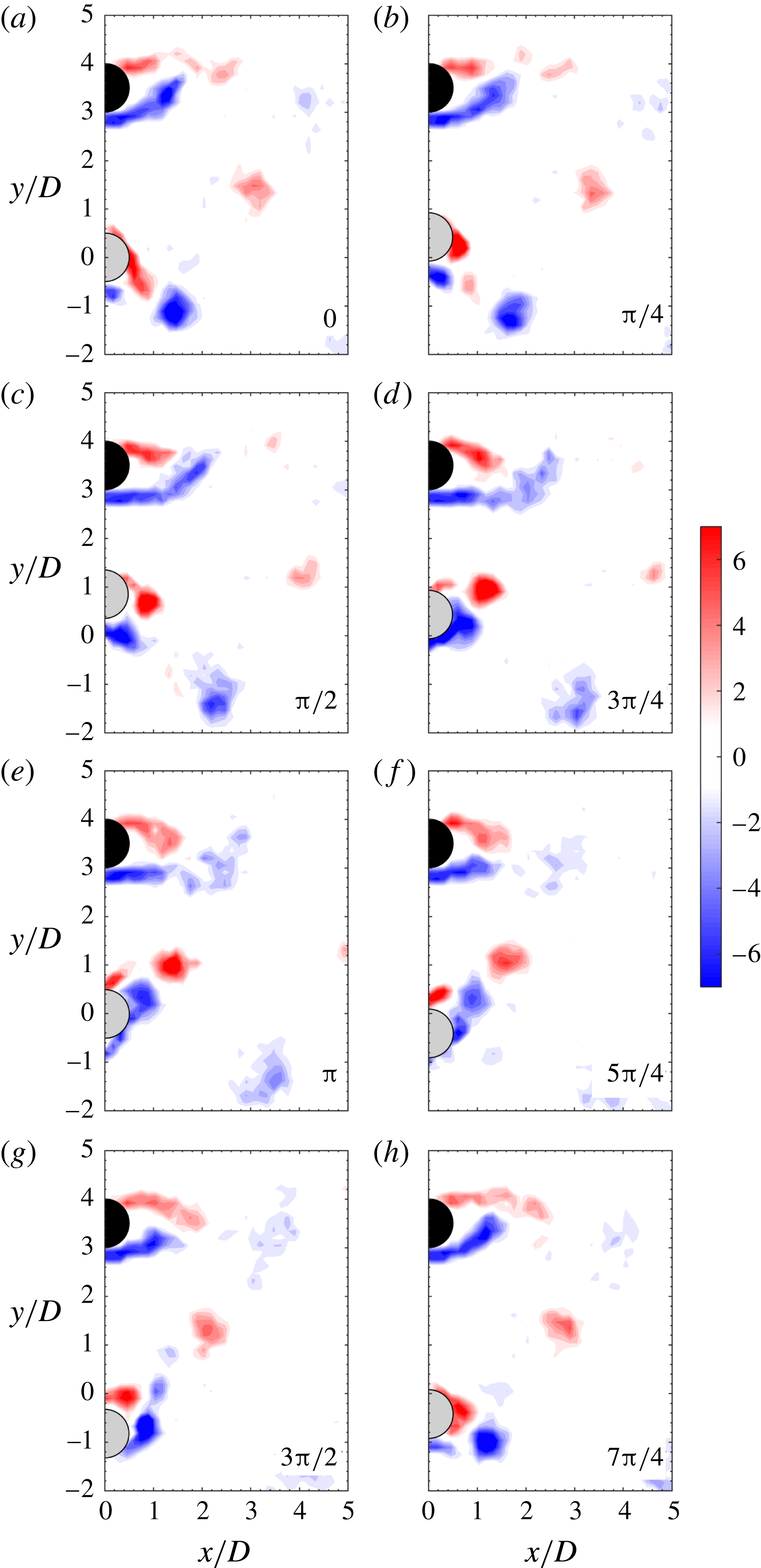
Phase-averaged dimensionless vorticity ( $\unicode[STIX]{x1D714}D/U$ ) for an experiment conducted with a separation of $3.5D$ and a reduced velocity $U^{\ast }\approx 5$ , at eight cylinder positions of the oscillation cycle. Flow is from left to right and the phases run from 0 to $7\unicode[STIX]{x03C0}/4$ , as labelled. Clockwise vorticity appears in red and anticlockwise vorticity apears in blue.

Figure 16.

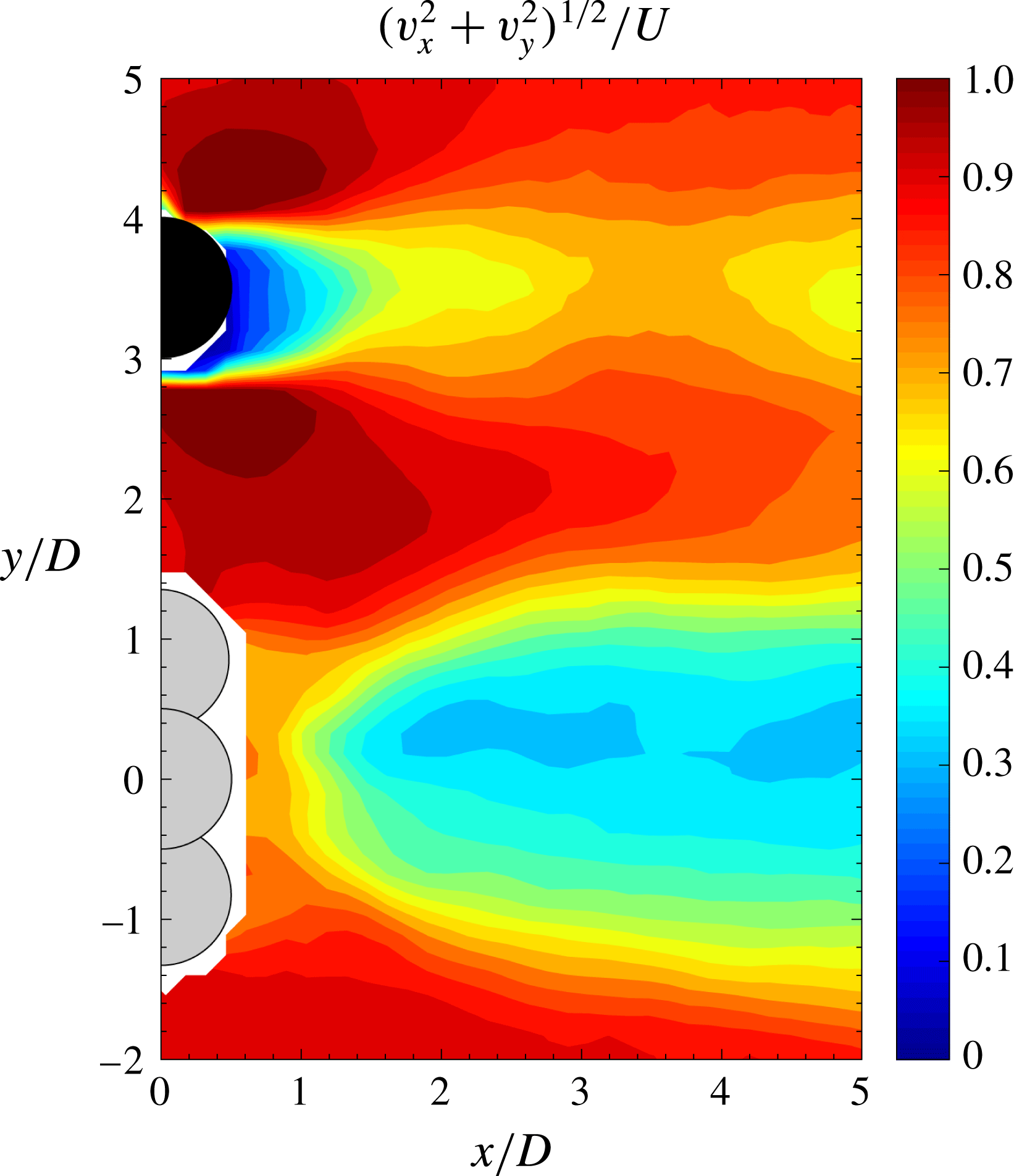
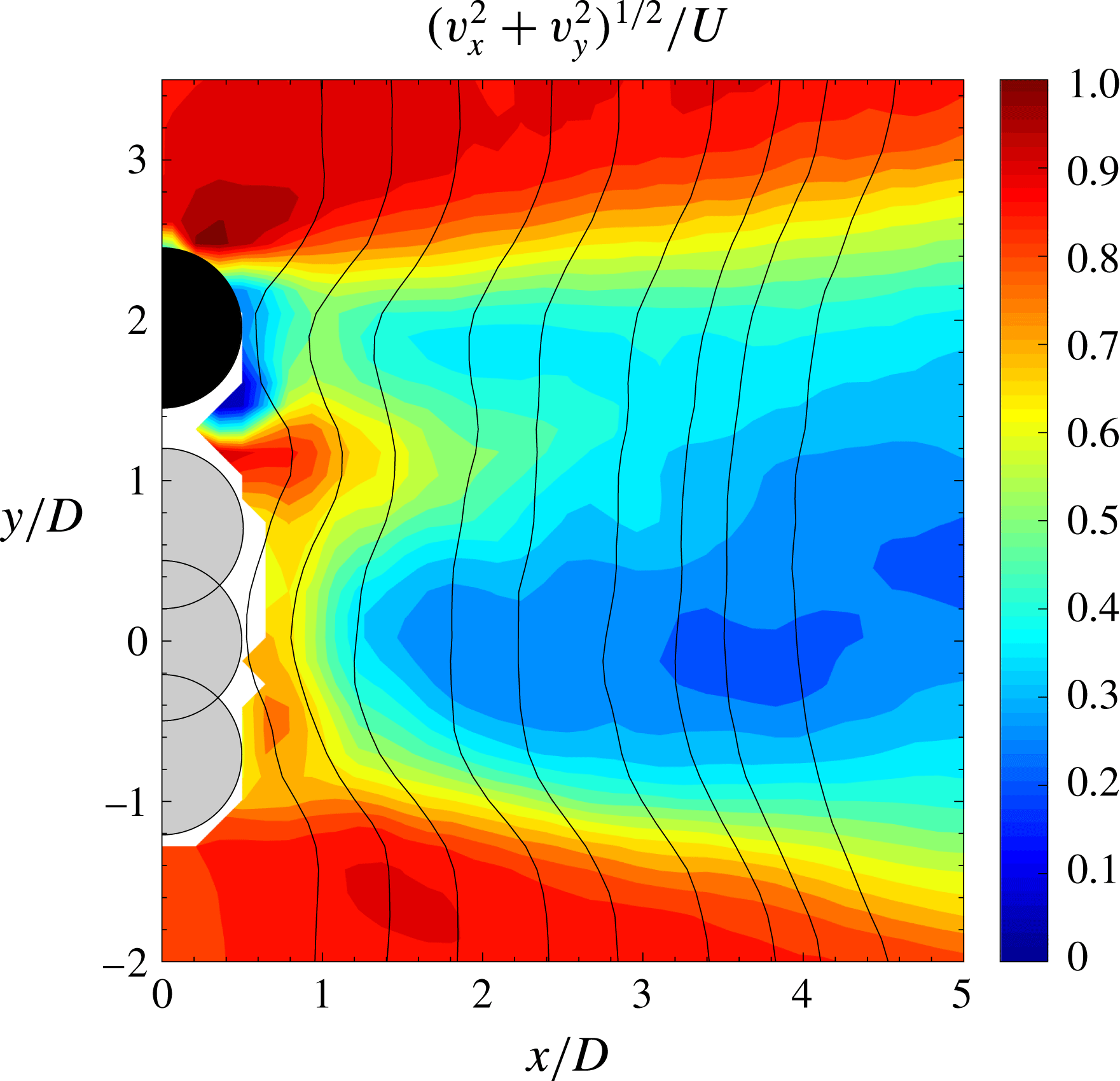
Time-averaged dimensionless magnitude of the velocity field $(U^{-1}\sqrt{v_{x}^{2}+v_{y}^{2}})$ for an experiment conducted with a separation of 3. $5D$ and a reduced velocity $U^{\ast }\approx 5$ .

At the largest separations, the wake of the oscillating cylinder resembles that typical of an isolated cylinder. Figure 15 shows the vorticity fields in the wake of the side-by-side cylinder arrangement, when separated by $3.5D$ at a reduced velocity near 5, where the largest amplitudes are expected, as seen in figure 2. The interference caused by the stationary cylinder is very weak, so although there is separated flow downstream of the stationary cylinder, the wake of the oscillating cylinder is mostly symmetric with respect to the $x$ axis. All phases show the same vortex topology behind the oscillating cylinder on both sides of the wake, indicating a minor influence of the stationary cylinder wake at this large separation. The time-averaged flow field in figure 16 shows a symmetrical structure, as well as the typical mean flow fields for a stationary and for a cylinder undergoing VIV. Shear layers in the near wake do not interact and the gap flow is characterised by magnitudes near those of the free stream. The same weak interaction is observed at reduced velocities outside the upper branch, as the motions of the vibrating cylinder are even smaller and therefore the time-varying distance between the cylinders is always larger, so the interaction is even less prominent.

Figure 17.

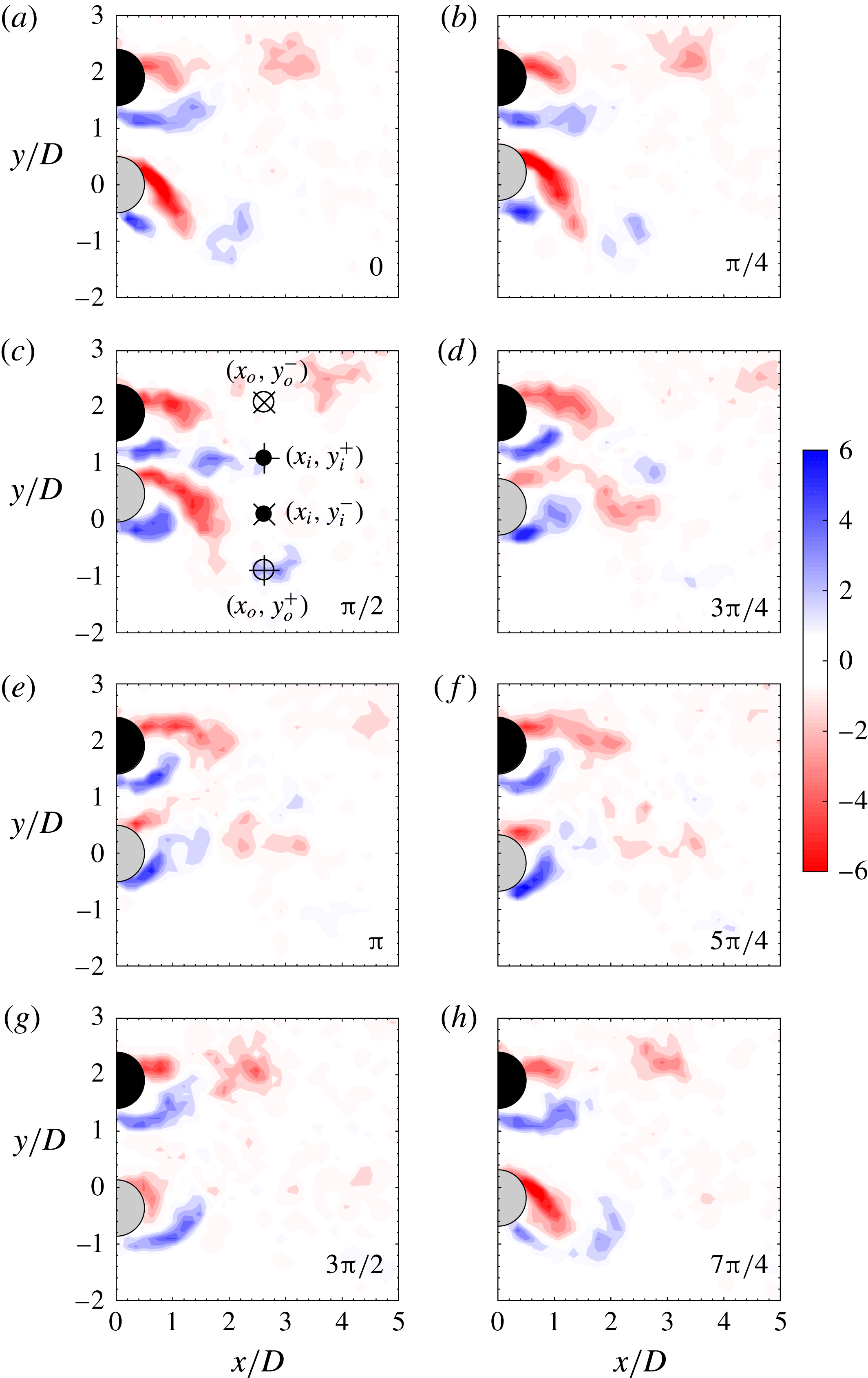
Phase-averaged dimensionless vorticity ( $\unicode[STIX]{x1D714}D/U$ ) for an experiment conducted with a separation of $2D$ and a reduced velocity $U^{\ast }\approx 5$ , at eight cylinder positions of the oscillation cycle. Flow is from left to right and the phases run from 0 to $7\unicode[STIX]{x03C0}/4$ , as labelled. Clockwise vorticity appears in red and anticlockwise vorticity apears in blue.

Figure 18.

Time-averaged dimensionless magnitude of the velocity field $(U^{-1}\sqrt{v_{x}^{2}+v_{y}^{2}})$ for an experiment conducted with separation of $2D$ and a reduced velocity $U^{\ast }\approx 5$ .

In figure 17 the dimensionless vorticity maps are shown for the case of the side-by-side arrangement with a centre-to-centre separation of $2D$ , in an experiment conducted at a $U^{\ast }\approx 5$ , in the upper branch where the oscillations measured were the largest (figures 3 and 4). The wake of both cylinders is synchronised in an out-of-phase fashion. A pair of counter-rotating vortices is formed in the gap region when the oscillating cylinder approaches the stationary cylinder, evolving in the near wake almost in parallel (panels c–e), with a small inclination towards the oscillating cylinder, until they completely dissipate (panel g). On the outer side of the wake, when the oscillating cylinder moves towards the stationary cylinder, a vortex is shed from the shear layer of each cylinder. The vortices shed from the stationary cylinder have lower levels of vorticity and dissipate before the ones shed from the oscillating cylinder. The latter ones have higher strength due to the larger circulation fed during its motion. The shape of the mean flow field region behind the cylinders, plotted in figure 18, confirms that the gap flow is biased to the oscillating cylinder. In this figure, solid lines have been added to the plot showing the velocity profile at positions from $1D$ to $4.5D$ behind the cylinder. The lines indicate the flow deflection to the vibrating cylinder part of the wake. The mean flow field differs radically if compared with the flow field presented before, for the same $U^{\ast }$ but with a separation of $3.5D$ (figure 16). The wakes are not independent and the shear layers have disappeared from the inner part of the wake, persisting only in the outer part, enclosing a large region of decelerated perturbed flow downstream in the models. Although in both cases the vibrating cylinder is oscillating with a similar amplitude, the gap between them when that cylinder is closer to the stationary one changes from more than $1.5D$ to approximately $0.3D$ , generating a gap flow that is heavily modified, that extends only $1D$ in the $x$ direction.

This mode of combined shedding resembles the out-of-phase coupled vortex shedding mode in the flow around two side-by-side stationary cylinders at moderate gap distances (Zdravkovich Reference Zdravkovich1997). Several authors have described this mode as a bistable mode (flip–flop), because when this almost symmetric type of shedding was observed around stationary cylinders, the deflection orientation of the wake changed from one cylinder to the other alternatingly (Bearman & Wadcock Reference Bearman and Wadcock1973; Sumner et al. Reference Sumner, Wong, Price and Païdoussis1999; Alam & Zhou Reference Alam and Zhou2007). Kim & Durbin (Reference Kim and Durbin1988) reported random changes in the inclination of the gap flow, at a frequency three orders of magnitude lower than that of the shedding process, between two deflected quasi-stable gap flow modes, through an unstable symmetric mode that stabilised only if external disturbances such as acoustic waves or a centre-line splitter plate were used. In contrast, Peschard & Le Gal (Reference Peschard and Le Gal1996) did not observe random flip–flop mode switching in their experiments and theoretical studies, and described how for gaps in the range from $2D$ to $3D$ , the wake was characterised by locked states corresponding to bistable regimes. They commented that the changes between the modes seemed not to be intrinsic to the wake but probably as a result of upstream perturbations in the form of turbulence. In all these works the gap distance was fixed; therefore, it was possible to identify well-delimited ranges for the gap in which the different behaviours were observed.

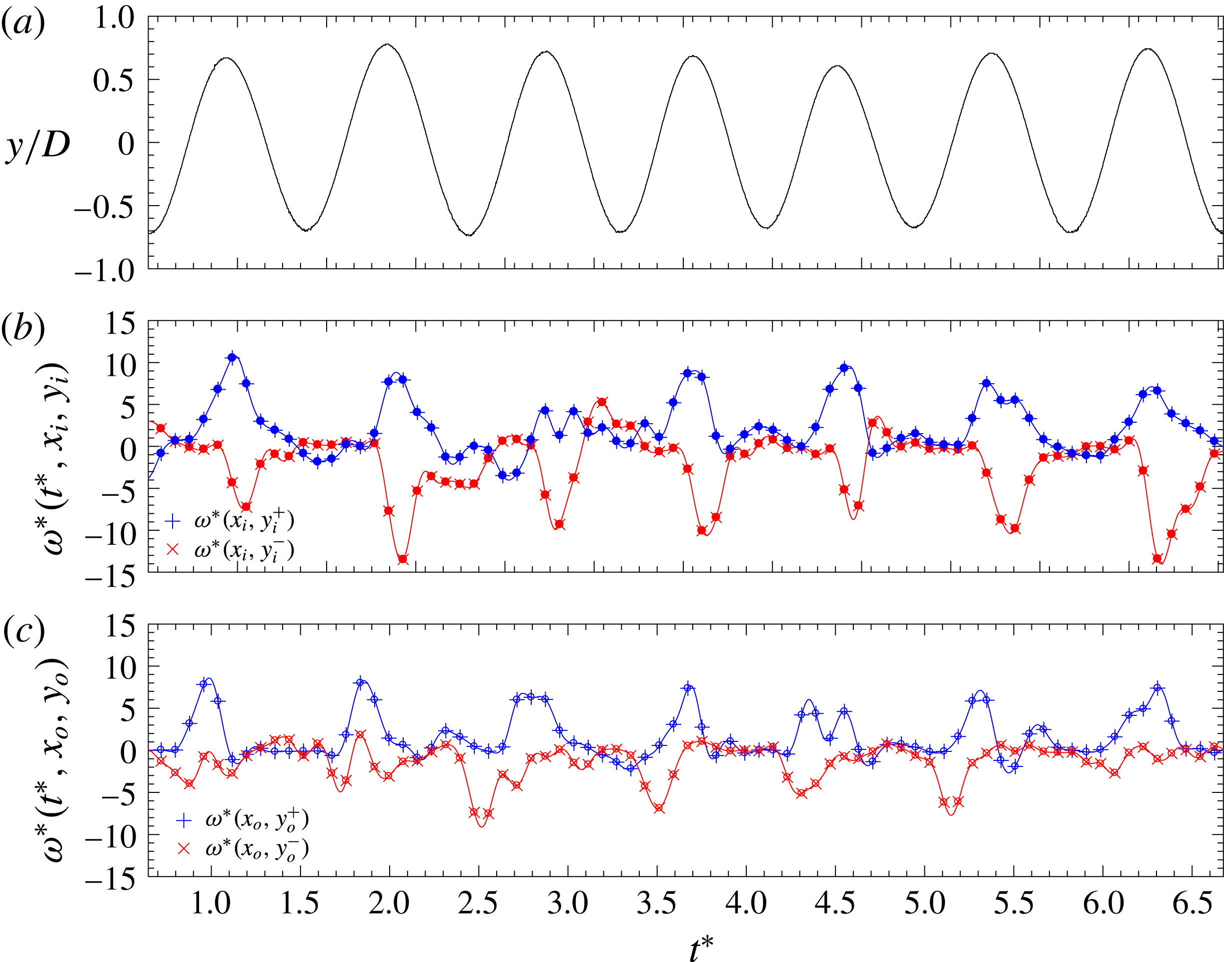
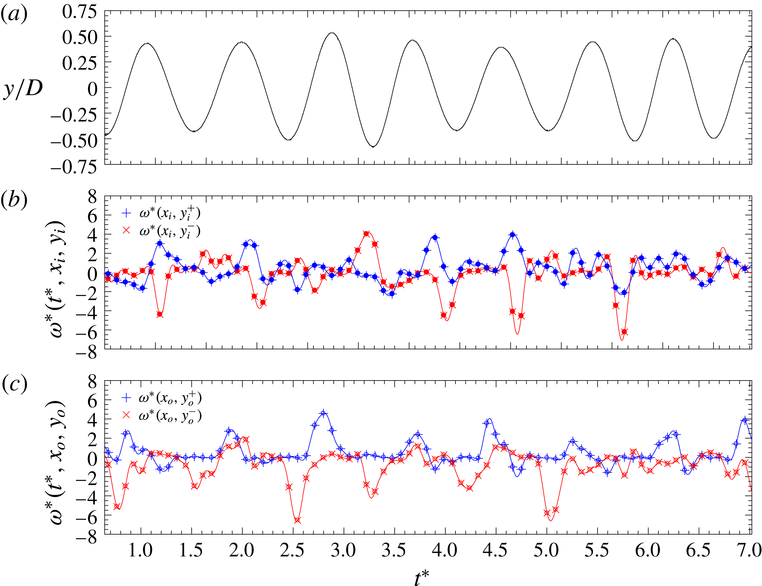
The time traces of the dimensionless vorticity at four positions in the wake of the case presented in figures 17 and 18 are shown in figure 19. All the data in the figures were extracted from the analysis of the DPIV flow fields and the displacement of the vibrating cylinder, from the DPIV image preprocessing. Figure 19(a) shows the motion of the cylinder. Figure 19(b) shows the time evolution of the vorticity at two points in the inner part of the wake in the gap flow region (solid dots). Figure 19(c) shows the vorticity at two points in the outer part of the wake (circles). The position of the probes appears indicated in figure 17(c) using the same symbols as in figure 19. Positive-signed vorticity (counterclockwise rotation) is indicated with a $+$ symbol and negative-signed vorticity is indicated with $\times$ . Solid symbols are used for the probes in the gap flow region and the circles for the probes in the outer part of the wake. Each peak in figure 19(b,c) indicates a vortex passing through the probe. In the gap flow, positive peaks are in advance of the negative ones, showing a phase difference, as described by Peschard & Le Gal (Reference Peschard and Le Gal1996), confirming the gap flow deflection towards the oscillating cylinder. In the outer part, the negative peaks are in advance of the positive ones, giving a flow orientation in the same direction as in the gap flow. Fourier analysis of the probe signals reveals that the vortex shedding is synchronised, with all signals having the same dominant frequency – that of the oscillation of the cylinder. This happens consistently in all the cycles presented in the plots of the figure, as well as in all the cases falling inside the lock-in region at this separation distance.

Figure 19.

Time series of the dimensionless vorticity at each of the probes that are indicated in figure 17(c).

The deflected mode of shedding with synchronised wakes is stable and seems to be an intrinsic characteristic of the experiments conducted with the smallest gaps, i.e. with strong wake interaction, at all the reduced velocities investigated inside the lock-in region. In this persisting out-of-phase mode, vortices result from the injection of momentum in the gap region to the inner shear layers. The motion of the cylinder besides the stationary one, generates a wake interaction that leads to the biased flow. Alam & Sakamoto (Reference Alam and Sakamoto2005) found in experiments conducted at $Re$ of the order of $10^{4}$ , how a small geometrical deviation in a stationary side-by-side arrangement (slightly staggered) resulted in a quasi-stable mode of shedding with a characteristic biased flow without mode switching. Previously, Wei & Chang (Reference Wei and Chang2002) found several stable deflected flow configurations using cross-sectional shape combinations in a pair of stationary side-by-side bluff bodies. They reported only one single bistable flip–flop configuration for the case of a square and circular cylinder side-by-side arrangement, for a very specific gap separation smaller than $1D$ .

In the present work, when the separation distance (dynamic separation) is small, the gap flow modifies the inner shear layers of both the stationary cylinder and the vibrating cylinder, substantially altering the vortex formation in the cylinders. The asymmetries observed in the velocity fields result from that modified vortex formation in the vibrating cylinder, with a frequency of shedding and a vortex strength that change if compared to the isolated case. These combined effects, caused by the altered shear layers through the gap flow, result in the stable deflected wake commented upon before. In Yildirim, Rindt & Steenhoven (Reference Yildirim, Rindt and Steenhoven2010), the authors used a control cylinder (with a very small diameter if compared to the main cylinder) placed at different near-wake locations and studied its effects on the wake of the larger cylinder. They found specific locations outside the wake of the cylinder in which the perturbation introduced by the control cylinder resulted in symmetry breaking and the appearance of a stable deflection in the wake. The authors attributed this effect to two factors: first, to the damping of the growth of disturbances, which in turn resulted in a modified shedding frequency, and second, to a modified vortex strength difference.

Moreover, the findings reported here are in agreement with the results obtained by Liu & Jaiman (Reference Liu and Jaiman2016), where the authors discussed thoroughly what was the cause for the flip–flop regime to disappear in the lock-in region in an arrangement of side-by-side cylinders, with one able to vibrate. The discussion, centred around a numerical scenario at very low $Re$ , was focused on the existence or not of two types of bifurcations near the critical $Re$ . The authors confirmed the existence of a quasi-stable deflected gap flow in the lock-in region and the absence of the flip–flop mode switching at the peak of the lock-in region, after detailed analysis of the phase of the transverse forces in both the stationary and the vibrating cylinder. More recently Liu & Jaiman (Reference Liu and Jaiman2018) have studied the same problem at moderate $Re$ , in order to see the effect of three dimensionality in the gap flow and in the flip–flop mode. Again, a deflected gap flow was observed inside the locked-in region with no flip–flop at the highest VIV response peak. Although the authors of these works report mode switching outside the locked-in peak of the response, their response curve is considerably narrower, meaning that, outside the peak, the amplitude falls very quickly. The bistable behaviour observed by Liu & Jaiman (Reference Liu and Jaiman2016) and Liu & Jaiman (Reference Liu and Jaiman2018) outside the lock-in peak seems to be inhibited in the present results by the fact that the oscillations of the vibrating cylinder extend over a wider range of velocities, and not only in a sharp response. This fact also gives an explanation for the increased response frequencies observed (see § 3), as the biased gap flow perturbs the inner shear layer of the moving cylinder, narrowing its wake and therefore enhancing the interaction with its outer shear layer, resulting in enhanced frequencies. As the cylinder oscillates, the circulation fed to the shear layers is larger than that being formed in the shear layers of the stationary cylinder. When the cylinder oscillates vigorously, finishing its motion near the stationary cylinder, the wakes are strongly synchronised in an out-of-phase fashion.

Figure 20.

Phase-averaged dimensionless vorticity ( $\unicode[STIX]{x1D714}/DU$ ) for an experiment conducted with separation of $2D$ and a reduced velocity $U^{\ast }\approx 7.5$ , at eight cylinder positions of the oscillation cycle. Flow is from left to right and the phases run from 0 to $7\unicode[STIX]{x03C0}/4$ , as labelled. Clockwise vorticity appears in red and anticlockwise vorticity apears in blue.

Figure 21.

Time series of the dimensionless vorticity at each of the probes that are indicated in figure 20(c).

In the lower branch of response with $S_{y}=2D$ , as seen in figure 20, the amplitudes have dropped considerably (see figure 3) and the instantaneous minimum gap is larger, hence the channelling effect and the momentum injection in the gap is less significant and the inner shear layer interaction is weakened, see panels (a) to (d). As a result, vortices in the gap region are more elongated if compared to the case presented in figure 17 and the frequencies of vortex shedding in the stationary and the moving cylinder are clearly different, with the wakes not synchronised and not keeping the same phase throughout the oscillation cycle. The mean flow for this case (not shown for the sake of brevity) shows a transitional situation between those reported in figures 18 and 16, with the inner shear layers interacting at approximately 2. $5D$ downstream in the models. Note that in the case of figure 16, with a larger separation between the models, the shear layer interaction happened far away from the models (outside the DPIV field of view), whilst in the case with the smallest $S_{y}$ in figure 18, the interaction takes place very near the gap. The time series of the vorticity signals output by the probes indicated in figure 20(c) appear in figure 21. The location of the probes in this case is different, because at the previous location the signals showed practically no peaks. The displacement of the vibrating cylinder in panel (a) is modulated in amplitude, and even looking for the most sensitive probe location, the time-varying vorticities in panels (b) and (c) do not show peaks with consistent phase differences. The same type of wake was observed in the lock-in region cases with separations of $2.5D$ and $3D$ , with the inner shear layer interaction happening further away from the models.

When the gap between the cylinders changes dynamically as in these experiments, it is very difficult to establish a precise value from which a strong wake interaction starts taking place, showing wake synchronisation and the stable deflected gap flow described. It is clear, however, that the size of the instantaneous gap distance is a key parameter, and it results not only from the separation configured at equilibrium, but also from the response, which depends on the specific reduced velocity set in each experiment. This time-varying separation defines how close to the models the inner shear layers interact, which has large effects on the response and on the characteristics of the gap flow. Note that for the cases with initial separation $S_{y}=2D$ , when the reduced velocities are approximately between 3.6 and 5.5, the response is always larger than $0.6D$ (with the maximum near $0.7D$ ), and the minimum instantaneous distance in the gap between the models, is in the range $0.3D$ to $0.4D$ . This small instantaneous gap promotes a strong wake interaction near the cylinders with synchronisation of frequencies and phases, leading to the stable deflected gap flow described before, as appears in figures 17 and 18. 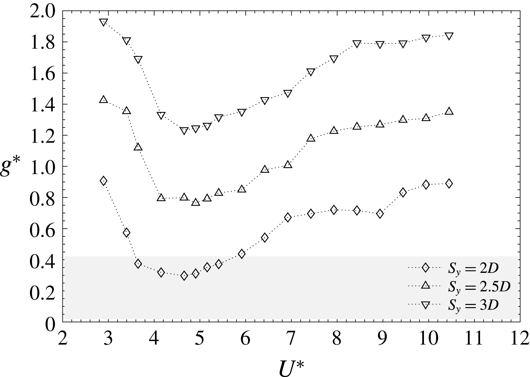On the other hand, in the lower branch cases, such as the one in figures 20 and 21, with amplitudes being roughly $0.45D$ , the minimum gap distance is larger (of the order of $0.6D$ or more), and wake synchronisation was not observed. In these cases, the wake interaction takes place further away from the cylinders. In figure 22 the gap between the cylinders (not the centre-to-centre separation, but the real separation between the cylinder’s surface), appears in dimensionless form computed as $g^{\ast }=S_{y}/D-(A^{\ast }+1)$ . Note that in the upper branch of the cases with $S_{y}=2.5D$ , $g^{\ast }$ are even larger than those in the lower branch of cases with separation $S_{y}=2D$ , and wake synchronisation was not observed. The grey region in the plot indicates the points in which synchronised wakes were observed together with deflected stable gap flows. The region is limited to the points with $S_{y}=2D$ that fell inside the lock-in region of the VIV response.

Figure 22.

Gap clearance $g^{\ast }$ between the cylinders as a function of $S_{y}$ and $U^{\ast }$ .