
1. Introduction
Accelerating wind energy deployment plays a vital role in the long-term reduction of greenhouse gas emissions. With the increasing scale and number of wind farms, flat terrain can no longer meet the construction needs of wind farms, and there is a high chance that they will be located on a non-flat complex terrain (Van Kuik et al. Reference Van Kuik2016). Compared with flat terrain, complex terrain will cause significant changes in the flow characteristics of the atmospheric boundary layer (Finnigan et al. Reference Finnigan, Ayotte, Harman, Katul, Oldroyd, Patton, Poggi, Ross and Taylor2020). As stated by Porté-Agel, Bastankhah & Shamsoddin (Reference Porté-Agel, Bastankhah and Shamsoddin2020), there are three key aspects of the flow over topography that potentially influence the evolution of wind-turbine wakes: namely, (i) non-zero pressure gradients, (ii) terrain-induced streamline distortion and (iii) flow separation. These complex flow patterns pose a significant challenge to the performance of wind-farm flow analytical models (WFFAMs) and significantly limit numerous engineering applications such as wind farm designs and micro-site selections over complex terrain.
To deal with these problems, many researchers have carried out related studies based on large-eddy simulation (LES), and the results show that streamline distortion and flow separation mainly affect the elevation of the wake-centre trajectory from the ground (e.g. Shamsoddin & Porté-Agel Reference Shamsoddin and Porté-Agel2018b; Liu, Lu & Ishihara Reference Liu, Lu and Ishihara2021; Zhang et al. Reference Zhang, Huang, Bitsuamlak and Cao2022b; Wang et al. Reference Wang, Feng, Peng, Mao, Doranehgard, Gupta, Li and Wan2023). Based on this physical insight, many WFFAMs are proposed to account for the baseflow streamline distortion induced by complex terrain. For instance, Feng, Shen & Li (Reference Feng, Shen and Li2018) assumed that the centreline of wind-turbine wakes is parallel to the topography, and their wake velocity deficit can be evaluated using the Jensen model. In addition, the sum of squares superposition method is used to calculate the velocity in the merged wake region. Finally, they proposed a WFFAM and applied it to wind farm layout optimisation in a realistic complex terrain. Unlike Feng et al. (Reference Feng, Shen and Li2018), Brogna et al. (Reference Brogna, Feng, Sørensen, Shen and Porté-Agel2020) assumed that the wake centreline coincides with the background streamline passing through the rotor centre, and the wake velocity deficit can be calculated using the Gaussian wake model. Recently, Farrell et al. (Reference Farrell, King, Draxl, Mudafort, Hamilton, Bay, Fleming and Simley2021) proposed a method that considers the heterogeneous background flow induced by complex terrain or mesoscale weather systems. Based on the Gaussian wake model, this method calculates the wake velocity deficit by dynamic coordinate transformation according to the baseflow streamline. Although this method has different computation details from Brogna et al. (Reference Brogna, Feng, Sørensen, Shen and Porté-Agel2020), its essence is still to assume that the wake centre evolves downstream along the streamline. It should be noted that this method has been integrated into the open-source software package FLORIS developed by NREL (Farrell et al. Reference Farrell, King, Draxl, Mudafort, Hamilton, Bay, Fleming and Simley2021).
However, none of the above-mentioned WFFAMs takes into account the influence of pressure gradient on wake evolution. The seminal work of Shamsoddin & Porté-Agel (Reference Shamsoddin and Porté-Agel2018a) shows that pressure gradient will significantly affect the wind turbine wake recovery and wake width. Under favourable pressure gradient (FPG), wind-turbine wakes will recover faster, whereas their recovery will slow down under adverse pressure gradient (APG). Therefore, pressure gradient is one of the most important but frequently ignored factors affecting the performance of WFFAMs over complex terrain, and there is an urgent need to develop WFFAMs under pressure gradient. In general, a complete WFFAM under pressure gradient should consist of two parts: the wake model and the wake superposition method (Porté-Agel et al. Reference Porté-Agel, Bastankhah and Shamsoddin2020). A large body of literature exists which focuses on these two parts individually, and they are introduced in the following.
1.1. Wake models under non-zero pressure gradient
Wake models describe the spatial distribution of wake velocity deficit downstream of the stand-alone wind turbine. The majority of wake models do not consider the influence of pressure gradient, so they are only applicable to flat terrain conditions and cannot be applied directly to WFFAMs under pressure gradient. As a result, this subsection focuses only on the wake models under pressure gradient. Readers interested in the zero-pressure-gradient (ZPG) wake models are referred to the related reviews (Crespo, Hernandez & Frandsen Reference Crespo, Hernandez and Frandsen1999; Stevens & Meneveau Reference Stevens and Meneveau2017; Archer et al. Reference Archer, Vasel-Be-Hagh, Yan, Wu, Pan, Brodie and Maguire2018, among others).
Based on the experimental observation that the ratio  $\lambda$ of the maximum velocity deficit
 $C$ to the wake width
 $\sigma$ is independent of the pressure gradient (Thomas & Liu Reference Thomas and Liu2004), Shamsoddin & Porté-Agel (Reference Shamsoddin and Porté-Agel2017, Reference Shamsoddin and Porté-Agel2018a) derived analytical wake models for the turbulent planar and axisymmetric wakes under pressure gradient for the first time. The derivation of the models takes advantage of the Bernoulli relation to replace the pressure gradient with the background velocity in the
 $x$-momentum equation. Moreover, it assumes the wake velocity deficit has a self-similar axisymmetric Gaussian distribution. Finally, a nonlinear ordinary differential equation (ODE) and an asymptotic solution for
 $C$ at each
 $x$-position are proposed based on the integral form of the
 $x$-momentum equation. Compared with the experimental and LES results, it is shown that the proposed models can accurately predict the influence of arbitrary pressure gradient on the evolution of the turbulent planar and axisymmetric wakes. Since turbulent axisymmetric wakes can be viewed as a simplification of wind-turbine wakes, the analytical model also applies to wind-turbine wakes (Shamsoddin & Porté-Agel Reference Shamsoddin and Porté-Agel2018b; Dar & Porté-Agel Reference Dar and Porté-Agel2022).
Based on this model, Dar & Porté-Agel (Reference Dar and Porté-Agel2022) further considered the pressure gradient induced by the wind rotor and proposed a new method to determine the initial value of velocity deficit in the near-wake region based on the Bernoulli equation, improving the performance of the model in escarpment cases. Recently, Dar, Gertler & Porté-Agel (Reference Dar, Gertler and Porté-Agel2023) systematically studied the effects of pressure gradients on some important wake characteristics, such as near-wake length and wake growth rate, using wind tunnel experiments on constant slope ramps with different inclination angles. It is shown that the analytical model designed for wakes under pressure gradient can improve the wake deficit prediction significantly when the ZPG wake model fails.
1.2. Wake superposition methods under ZPG
When a specific location in the wind farm is affected by the wakes of more than one wind turbine, the wake velocity deficit at that location needs to be determined by wake superposition methods. The wake superposition method is an essential factor affecting the performance of WFFAMs, and existing wake superposition methods are all proposed for the ZPG condition (Porté-Agel et al. Reference Porté-Agel, Bastankhah and Shamsoddin2020). Early wake superposition models are all empirical expressions without solid theoretical foundations. Lissaman (Reference Lissaman1979) assumed that the distance between wind turbines in a wind farm is large, and thus the wake interference is minimal. Therefore, the velocity deficit can be regarded as a passive scalar, and the cumulative wake velocity deficit generated by multiple wind turbines is similar to the pollutant concentration of multiple plumes. Based on this assumption, the merged wake velocity deficit can be obtained by linearly superposing the velocity deficits generated by different wind turbines. In contrast, Katic, Højstrup & Jensen (Reference Katic, Højstrup and Jensen1986) assumed that the total kinetic energy deficit within the superposition region is equal to the accumulation of individual wake kinetic energy deficits, and they proposed the widely used sum of squares superposition principle. It is noteworthy that the two described superposition methods calculate the wake velocity deficit or kinetic energy deficit based on the freestream wind speed  $U_\infty$, which may lead to the overestimation of these two quantities of the waked turbine. To this end, Voutsinas, Rados & Zervos (Reference Voutsinas, Rados and Zervos1990) developed a new wake superposition method based on the sum of squares superposition of the local kinetic energy deficits, which are defined by the local incoming flow speed
 $u_0^i$ for the
 $i$th turbine. Similarly, Niayifar & Porté-Agel (Reference Niayifar and Porté-Agel2016) use
 $u_0^i$ as the reference speed to calculate the local velocity deficits but linearly superimpose them to calculate wind-farm flows. According to the different definitions of the velocity deficit caused by the
 $i$th turbine and different superposition principles, the wind-farm flow velocity deficit
 $U_s$ obtained by the four described superposition methods are denoted and written as follows:
 \begin{align} &\text{Global linear:} \quad U_s(x,y,z)=\sum_i(U_\infty-u_w^i(x,y,z)), \end{align}
 \begin{align} &\text{Global square:}\quad U_s(x,y,z)=\sqrt{\sum_i(U_\infty-u_w^i(x,y,z))^2}, \end{align}
 \begin{align} &\text{Local linear:}\quad U_s(x,y,z)=\sum_i( u_0^i-u_w^i(x,y,z)), \end{align}
 \begin{align} &\text{Local square:}\quad U_s(x,y,z)=\sqrt{\sum_i( u_0^i-u_w^i(x,y,z))^2}. \end{align}
Here,  $u_w^i$ represents the wake velocity of the
 $i$th wind turbine and can be calculated through the wake model.
Recently, Lanzilao & Meyers (Reference Lanzilao and Meyers2022) proposed a novel recursive relation capable of merging wind-turbine wakes, which can be called wind product:
 \begin{equation} \text{Wind product:}\quad U_s(x,y,z)=U_\infty-U_\infty\prod_i\left(\frac{u_w^i(x,y,z)}{u_0^i}\right). \end{equation}
By comparing its prediction with LES and supervisory control and data acquisition data, they found that the performance of this wake superposition method is very close to the local linear method, with a similar mean absolute error (MAE) in a homogeneous background velocity field, whereas it displays a lower MAE in the case of a heterogeneous background velocity, which may be applicable for the cases under pressure gradient. It is noteworthy that the wind product method has a different form from the other superposition methods. As shown in (1.1)–(1.4), the total wind-farm flow velocity deficit  $U_s$ is calculated as the sum of individual velocity deficits in a specific way. In contrast, the wind product method directly calculates the wind-farm flow
 $U_w$ as a product of
 $U_\infty$ with normalised individual wake velocity of each turbine. Finally,
 $U_s$ is obtained by subtracting
 $U_w$ from the base flow
 $U_\infty$.
Although these superposition models claim to conserve momentum or energy deficit, they make many unreasonable assumptions, so they are all empirical methods that need to be improved. To this end, Zong & Porté-Agel (Reference Zong and Porté-Agel2020) proposed a superposition method that conserves the total momentum deficit in the streamwise direction for the first time. By defining the mean wake convection velocity  $u_c^i (x)$ and
 $U_c(x)$ of the single-alone wind turbine wake and the combined wake, respectively, a linear weighted wake superposition method is proposed. The weight of the contribution of the
 $i$th wind turbine to the wind farm is
 $u_c^i (x)/U_c(x)$. The expression is as follows:
 \begin{equation} \text{IMCM:}\quad U_s(x,y,z)=\sum_i\frac{u_c^i(x)}{U_c(x)}(u_0^i-u_w^i(x,y,z)). \end{equation}
Since the determination of  $U_c(x)$ relies on
 $U_s$ and
 $U_\infty -U_s$, this method needs an iterative method (Zong & Porté-Agel Reference Zong and Porté-Agel2020). Therefore, we denote it as the implicit momentum-conserving method (IMCM). Compared with wind tunnel measurements and LES results, this method outperforms all the empirical methods by accurately predicting the power production and the centreline wake velocity deficit (Zong & Porté-Agel Reference Zong and Porté-Agel2020).
In addition, Bastankhah et al. (Reference Bastankhah, Welch, Martínez-Tossas, King and Fleming2021) developed a fairly simple explicit relationship that predicts the streamwise velocity distribution within a wind farm by solving an approximate form of conservation of mass and momentum for a turbine in a wind farm array (Bay et al. Reference Bay, Fleming, Doekemeijer, King, Churchfield and Mudafort2023; Blondel Reference Blondel2023). As this model is obtained by solving flow-governing equations directly for a turbine that is subject to upwind turbine wakes, no ad hoc superposition technique is needed to predict wind-farm flows. Therefore, this model essentially differs from the superposition methods introduced above, which rely on the stand-alone wake model. Here, we do not intend to account for the effect of pressure gradient by explicitly solving the integral Reynolds-averaged Navier–Stokes (RANS) equation, which is far beyond the scope of this study.
1.3. The present work
In summary, previous studies mainly focused on the wake model under pressure gradient and wake superposition methods under the ZPG condition. Until recently, Dar & Porté-Agel (Reference Dar and Porté-Agel2024) proposed to extend the application of the analytical wake model under pressure gradient to multiple turbine wakes by updating the effective background velocity for wind turbines from upstream to downstream. Although their method has only been validated in the aligned layout, it can be extended to arbitrary wind-farm layouts with minor modifications. From the perspective of wake superposition, their method is very similar to the wind product method proposed by Lanzilao & Meyers (Reference Lanzilao and Meyers2022) but accounts for the influence of pressure gradient on the single-wake evolution. Nevertheless, the research on the wake superposition method and WFFAM under pressure gradient is still at a very early stage, and there is much work that needs to be done. As demonstrated by Zong & Porté-Agel (Reference Zong and Porté-Agel2020) and Bastankhah et al. (Reference Bastankhah, Welch, Martínez-Tossas, King and Fleming2021), the momentum-conserving methods under the ZPG condition have superior performance compared with empirical superposition methods. Therefore, a momentum-conserving method under pressure gradient is the focus of this study, which has not been proposed previously. Specifically, we theoretically derive an implicit momentum-conserving wake superposition model under pressure gradient (PG-IMCM), show its simplified form and validate their performance against high-fidelity LES results. Moreover, five empirical WFFAMs under pressure gradient based on (1.1)–(1.5) are further developed and inter-compared.
The remainder of the article is as follows. The model development is elaborated on in § 2. In § 3, the LES methodology and validation cases set-up are introduced. The performance of the momentum-conserving method is validated in § 4. In § 5, we further extend the empirical superposition methods to account for pressure gradient and compare their performance against LES results. Finally, conclusions are given in § 6.
2. Model development
In this section, we show the proposed momentum-conserving WFFAM under pressure gradient with an emphasis on the derivation of the implicit momentum-conserving wake superposition model under pressure gradient (PG-IMCM) in § 2.1. The single turbine wake model under pressure gradient is given in § 2.2. Moreover, a simplified version of PG-IMCM is presented in § 2.3.
2.1. Theoretical derivation of PG-IMCM
2.1.1. Total momentum deficit under pressure gradient
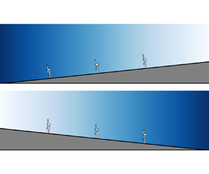
Here, we consider a wind farm with  $N$ wind turbines
 $(WT_1,\ldots,WT_i,\ldots,WT_N)$ under pressure gradient with the base flow
 $U_b(x)$, as depicted in figure 1. The wind turbines are assumed to have the same rotor diameter
 $D$. The position of
 $WT_i$ is labelled as
 $(x_i,y_i,z_i)$, where
 $x$,
 $y$ and
 $z$ are the streamwise, spanwise and vertical coordinates, respectively. Wind turbines are ordered with respect to their streamwise positions to ensure
 $x_i\geq x_{i-1}$. The RANS streamwise momentum equation for wind-farm flows can be written as follows:
 \begin{equation} U_w\frac{\partial U_w}{\partial x}+V\frac{\partial U_w}{\partial y}+W\frac{\partial U_w}{\partial z}={-}\frac{1}{\rho}\frac{\partial P}{\partial x}-\frac{\partial \overline{u^\prime u^\prime}}{\partial x}-\frac{\partial \overline{u^\prime v^\prime}}{\partial y}-\frac{\partial \overline{u^\prime w^\prime}}{\partial z}+\frac{f_t}{\rho}. \end{equation}
Here,  $U_w$,
 $V$ and
 $W$ are the streamwise, spanwise and vertical velocity of the wind-farm flow, respectively,
 $\overline {u^\prime u^\prime }$,
 $\overline {u^\prime v^\prime }$ and
 $\overline {u^\prime w^\prime }$ are the Reynolds stress components,
 $P$ is the time-averaged static pressure,
 $\rho$ is the air density and
 $f_t$ is the body force caused by wind turbines, which can be expressed as (Bastankhah et al. Reference Bastankhah, Welch, Martínez-Tossas, King and Fleming2021):
 \begin{equation} \frac{f_t}{\rho}=\sum_{i=1}^N-\frac{T_i}{\rho\pi R^2}\delta(x-x_i)\mathcal{H}(R^2-[(y-y_i)^2+(z-z_i)^2]), \end{equation}
where  $T_i$ is the thrust of
 $WT_i$,
 $R$ is the rotor radius,
 $\delta (x)$ is the Dirac delta function and
 $\mathcal {H}(x)$ is the Heaviside step function. The viscous term is neglected due to the high Reynolds number in the atmospheric boundary layer. It is noteworthy that we only consider the background pressure variations induced by complex terrain and neglect the sudden pressure changes in the near-wake region of the wind rotor (Dar & Porté-Agel Reference Dar and Porté-Agel2022). Therefore, the streamwise pressure gradient
 $\partial P/\partial x$ and the streamwise variation of the background velocity
 $U_b(x)$ satisfy the Bernoulli equation under the considered conditions, i.e.
 $1/\rho \partial P/\partial x=-({\rm d}U_b/{{\rm d}\kern0.7pt x})U_b$. The governing equation for the wind-farm flow velocity deficit
 $U_s(x,y,z)=U_b(x)-U_w(x,y,z)$ can be derived by subtracting (2.1) from
 $U_w \partial U_b/\partial x$, with the assumption of
 $\partial U_b/\partial y=\partial U_b/\partial z=0$:
 \begin{equation} U_w\frac{\partial U_s}{\partial x}+V\frac{\partial U_s}{\partial y}+W\frac{\partial U_s}{\partial z}={-}\frac{{\rm d} U_b}{{\rm d}\kern0.7pt x}U_s+\frac{\partial \overline{u^\prime u^\prime}}{\partial x}+\frac{\partial \overline{u^\prime v^\prime}}{\partial y}+\frac{\partial \overline{u^\prime w^\prime}}{\partial z}-\frac{f_t}{\rho}. \end{equation}
In addition, considering the continuity equation,
 \begin{equation} \frac{\partial U_w}{\partial x}+\frac{\partial V}{\partial y}+\frac{\partial W}{\partial z}=0, \end{equation}
we can obtain the following:
 \begin{equation} U_w\frac{\partial U_s}{\partial x}+V\frac{\partial U_s}{\partial y}+W\frac{\partial U_s}{\partial z}=\frac{\partial U_w U_s}{\partial x}+\frac{\partial VU_s}{\partial y}+\frac{\partial WU_s}{\partial z}. \end{equation}
Substituting (2.5) into (2.3) yields
 \begin{equation} \frac{\partial U_wU_s}{\partial x}+\frac{\partial VU_s}{\partial y}+\frac{\partial WU_s}{\partial z}={-}\frac{{\rm d} U_b}{{\rm d}\kern0.7pt x}U_s+\frac{\partial \overline{u^\prime u^\prime}}{\partial x}+\frac{\partial \overline{u^\prime v^\prime}}{\partial y}+\frac{\partial \overline{u^\prime w^\prime}}{\partial z}-\frac{f_t}{\rho}. \end{equation}
Then, we can take the  $y$–
 $z$ plane integral from
 $x_0$ (a location upstream of the wind farm) to
 $x$ (an arbitrary location within or downstream of the wind farm). The upper and lower bounds of the
 $y$- and
 $z$-integration are selected far from the wind farm to ensure
 $U_s$,
 $\overline {u^\prime v^\prime }$ and
 $\overline {u^\prime w^\prime }$ all vanish (in a given
 $x$-normal plane). Therefore, the integrals of the terms inclusive of the
 $y$- or
 $z$-derivative in (2.6) are zero. In addition, the integral of normal Reynolds stress component
 $\iint \overline {u^\prime u^\prime }\,{\rm d}\kern 0.05em y\,{\rm d}z|_{x_0}^x$ is negligible, compared with other terms according to the budget comparison of Bastankhah et al. (Reference Bastankhah, Welch, Martínez-Tossas, King and Fleming2021). Therefore, the final expression for the total momentum deficit under pressure gradient is
 \begin{align} &\iint U_w(x,y,z)[U_b(x)-U_w(x,y,z)]\,{\rm d}\kern0.05em y\,{\rm d}z\nonumber\\ &\quad =\sum_{i\in B}\frac{T_i}{\rho}-\iint \underbrace{\int_{x_0}^{x}\frac{{\rm d}U_b(x^\prime)}{{{\rm d}\kern0.7pt x}^\prime}U_s(x^\prime, y,z)\,{{\rm d}\kern0.7pt x}^\prime}_{{\mathfrak P}(x,y,z)} \,{{\rm d}\kern0.05em y}\,{\rm d}z. \end{align}
Here,  $B=\{i\,|\,x_i< x\}$ and
 ${\mathfrak P}(x,y,z)$ is the pressure correction term induced by the wind-farm velocity deficit. The equation shows that the total momentum deficit for a wind farm under pressure gradient consists of two parts: the total thrust of wind turbines and the integral of
 ${\mathfrak P}(x,y,z)$, which is related to the pressure gradient.
Schematic of a wind farm with an arbitrary layout consisting of  $N$ wind turbines under FPG. (Dark blue represents the high-pressure region, whereas light blue represents the low-pressure region.)

2.1.2. General expression for the wind-turbine thrust under pressure gradient
To proceed with our derivation, we introduce some new velocity variables. To begin with, we give the rules of nomenclature as follows:  $u^i$ represents the velocity variables of
 $WT_i$, whereas
 $U^i$ represents the velocity variables associated with
 $i$ wind turbines; The subscripts
 $s$,
 $w$ and
 $b$ represent the velocity deficit, the wake velocity and the base flow, respectively. By definition,
 $U_b^i=U_b$. Subsequently, we choose two control volumes, including
 $i$ and
 $i-1$ wind turbines, whose upper bound of the streamwise coordinate is larger than
 $x_i$. The only difference is that the latter excludes
 $WT_i$, as depicted in figure 2. In this condition, if we apply (2.7) to these two control volumes and subtract one from the other, we can obtain the expression for the thrust of
 $WT_i$ as follows:
 \begin{align} \frac{T_i}{\rho}&=\iint U_w^i(x,y,z)[U_b(x)-U_w^i(x,y,z)]\,{\rm d}\kern0.05em y\,{\rm d}z\nonumber\\ &\quad -\iint U_w^{i-1}(x,y,z)[U_b(x)-U_w^{i-1}(x,y,z)]\,{\rm d}\kern0.05em y\,{\rm d}z \nonumber\\ &\quad +\iint \int_{x_i-\delta x}^{x}\frac{{\rm d}U_b(x^\prime)}{{{\rm d}\kern0.7pt x}^\prime}[U_w^{i-1}(x^\prime, y,z)-U_w^i(x^\prime, y,z)]\,{{\rm d}\kern0.7pt x}^\prime\, {{\rm d}\kern0.05em y} \,{\rm d}z, \end{align}
where  $\delta _x$ represents an infinitely small distance,
 $U_w^i$ and
 $U_w^{i-1}$ are the streamwise velocity of the wind-farm flow with
 $i$ wind turbines and
 $i-1$ wind turbines, respectively. Here
 $U_w^{i-1}-U_w^i$ is essentially the wake velocity deficit
 $u_s^i$ induced by
 $WT_i$, which can be modelled by the wake model under pressure gradient. As has been demonstrated by Bastankhah et al. (Reference Bastankhah, Welch, Martínez-Tossas, King and Fleming2021), the first and second terms on the right-hand side of (2.8) can be simplified as follows:
 \begin{align} &\iint U_w^i[U_b(x)-U_w^i]\,{\rm d}\kern0.05em y\,{\rm d}z-\iint U_w^{i-1}[U_b(x)-U_w^{i-1}]\,{\rm d}\kern0.05em y\,{\rm d}z\nonumber\\ &=\iint U_w^i(U_w^{i-1}-U_w^i)\,{\rm d}\kern0.05em y\,{\rm d}z-\iint (U_w^{i-1}-U_w^i)[U_b(x)-U_w^{i-1}]\,{\rm d}\kern0.05em y\,{\rm d}z \nonumber\\ &\leq \iint U_w^i(U_w^{i-1}-U_w^i)\,{\rm d}\kern0.05em y\,{\rm d}z=\iint (U_w^{i-1}-u_s^i)u_s^i\,{\rm d}\kern0.05em y\,{\rm d}z. \end{align}
Generally speaking,  $U_w^{i-1}(x,y,z)$ is a three-dimensional spatial-varying velocity distribution, which is influenced by the cumulative effect of
 $i-1$ wind-turbine wakes and is essentially the base flow for
 $WT_i$. To further simplify our derivation, we assume the use of
 $u_b^i(x)$ to replace
 $U_w^{i-1}$. It should be noted that
 $u_b^i(x)$ may differ significantly from
 $U_b(x)$ depending on the wind-farm layout, as it can be influenced by upstream wind-turbine wakes. As a result, the modified momentum deficit can be approximated as follows:
 \begin{equation} \iint (U_w^{i-1}-u_s^i)u_s^i\,{\rm d}\kern0.05em y\,{\rm d}z \approx \iint [u_b^i(x)-u_s^i]u_s^i\,{\rm d}\kern0.05em y\,{\rm d}z, \end{equation}
where  $u_b^i(x)-u_s^i=u_w^i$ is the wake velocity of
 $WT_i$ accounting for the base flow variation.
Schematic of the control volume for (a)  $i$ wind turbines and (b)
 $i-1$ wind turbines under FPG. (b) is the same as (a) in the absence of
 $WT_i$.

In our study,  $u_b^i(x)$ is modelled as the average wind speed in the rotor area behind
 $WT_i$, which is sampled in
 $U_w^{i-1}$ to represent different wake interference conditions, such as full wake and partial wake. To save computational costs, we approximate
 $u_b^i(x)$ using the average of
 $N_q=16$ velocity sampling lines downstream of
 $WT_i$, whose spanwise and vertical coordinates (
 $y_{i,q}$ and
 $z_{i,q}$) are the same as the quadrature points evenly divided over the rotor area of
 $WT_i$, as shown in figure 3. The coordinates of the quadrature points can be found in Allaerts & Meyers (Reference Allaerts and Meyers2019), which is adopted to calculate the rotor equivalent wind speed. The expression for
 $u_b^i(x)$ is defined as follows:
 \begin{equation} u_b^i(x)=\frac{1}{N_q}\sum_{q=1}^{N_q}U_w^{i-1}(x,y_{i,q},z_{i,q}) =U_b(x)-\frac{1}{N_q}\sum_{q=1}^{N_q}U_s^{i-1}(x,y_{i,q},z_{i,q}). \end{equation}
Schematic of (a) quadrature points at the rotor plane of  $WT_i$ and (b) velocity sampling lines of
 $WT_i\ (i\geq 2)$.

For  $i=1$,
 $u_b^1(x)=U_b(x)$, whereas for
 $i\geq 2$,
 $u_b^i(x)$ can be obtained through a recursive procedure, which is detailed in Appendix A. It should be noted that this modelling for
 $u_b^i(x)$ is different from Dar & Porté-Agel (Reference Dar and Porté-Agel2024), who use the wind speed in the wake centreline behind
 $WT_i$ as
 $u_b^i(x)$, which may be only applicable for the aligned wind farm layout. In contrast, our proposed modelling for
 $u_b^i(x)$ can be applicable for arbitrary wind farm layouts.
Finally, the thrust of  $WT_i$ can be expressed as
 \begin{align} \frac{T_i}{\rho}&=\iint u_w^i(x,y,z)[u_b^i(x)-u_w^i(x,y,z)]\,{\rm d}\kern0.05em y\,{\rm d}z\nonumber\\ &\quad +\iint \underbrace{\int_{x_i-\delta x}^{x}\frac{{\rm d}U_b(x^\prime)}{{{\rm d}\kern0.7pt x}^\prime}u_s^i(x^\prime, y,z)\,{{\rm d}\kern0.7pt x}^\prime}_{{\mathfrak p}^i(x,y,z)} {{\rm d}\kern0.05em y} \,{\rm d}z. \end{align}
Here,  ${\mathfrak p}^i(x,y,z)$ is the pressure correction term induced by individual velocity deficit.
2.1.3. Linearised expression for the wind-turbine thrust under pressure gradient
It has been shown that the wake velocity deficit  $u_s^i$ under pressure gradient has a Gaussian distribution, but with different normalised maximum velocity deficit
 $C^i(x)$ and wake width
 $\sigma ^i(x)$ from its counterpart under ZPG (Shamsoddin & Porté-Agel Reference Shamsoddin and Porté-Agel2018a). Therefore,
 $u_s^i$ and
 $u_w^i$ for
 $WT_i$ can be expressed as:
 $$\begin{gather} u_s^i(x,y,z)=u_b^i(x)C^i(x)\exp\left(-\frac{(y-y_i)^2+(z-z_i)^2}{2\sigma^{i}(x)^2}\right), \end{gather}$$
 $$\begin{gather}u_w^i(x,y,z)=u_b^i(x)\left[1-C^i(x)\exp\left(-\frac{(y-y_i)^2+(z-z_i)^2}{2\sigma^{i}(x)^2}\right)\right]. \end{gather}$$
We give  $C^i(x)$ and
 $\sigma ^i(x)$ in § 2.2, and for now they are assumed to be known. The first term on the right-hand side of (2.12) can be linearised by introducing a convection velocity
 $u_c^i(x)$ (Zong & Porté-Agel Reference Zong and Porté-Agel2020), and it can be given analytically as
 \begin{equation} u_c^i(x)=\frac{\displaystyle\iint u_w^i(x,y,z)[u_b^i(x)-u_w^i(x,y,z)]\,{\rm d}\kern0.05em y\,{\rm d}z}{\displaystyle\iint [u_b^i(x)-u_w^i(x,y,z)]\,{\rm d}\kern0.05em y\,{\rm d}z}=u_b^i(x)\left(1-\frac{C^i(x)}{2}\right). \end{equation}
Therefore, the expression for the thrust of  $WT_i$ under pressure gradient can be rewritten as
 \begin{align} \frac{T_i}{\rho}=\underbrace{u_c^i(x)\iint [u_b^i(x)-u_w^i(x,y,z)]\,{\rm d}\kern0.05em y\,{\rm d}z}_{T_{MD}^i(x)}+\underbrace{\iint \int_{x_i-\delta x}^{x}\frac{{\rm d}U_b(x^\prime)}{{{\rm d}\kern0.7pt x}^\prime}u_s^i(x^\prime, y,z)\,{{\rm d}\kern0.7pt x}^\prime \,{{\rm d} y} \,{\rm d}z}_{T_{\mathfrak p}^i(x)}. \end{align}
This equation indicates that for  $WT_i$ operating under pressure gradient, its thrust can be decomposed into two parts: the linearised momentum deficit flux
 $T_{MD}^i$ and the integral of
 ${\mathfrak p}^i(x,y,z)$ (i.e.
 $T_{{\mathfrak p}}^i$), which is related to pressure gradient. In the derivation of (2.12) and (2.16), we have made some assumptions, such as the utilisation of the modified momentum deficit and the substitution of
 $U_w^{i-1}$ by
 $u_b^i(x)$. However, these simplifications only lead to negligible errors based on the comparison between the modelled wind turbine thrust and LES results shown in § 4, indicating that these assumptions are reasonable.
2.1.4. PG-IMCM superposition method
Substituting (2.16) into (2.7) yields
 \begin{align} &\iint U_w(x,y,z)[U_b(x)-U_w(x,y,z)]\,{\rm d}\kern0.05em y\,{\rm d}z \nonumber\\ &\quad= \sum_{i\in B}u_c^i(x)\iint[u_b^i(x)-u_w^i(x,y,z)]\,{\rm d}\kern0.05em y\,{\rm d}z \nonumber\\ &\qquad +\sum_{i\in B}\iint \underbrace{\int_{x_i-\delta x}^{x}\frac{{\rm d}U_b(x^\prime)}{{{\rm d}\kern0.7pt x}^\prime}u_s^i(x^\prime, y,z)\,{{\rm d}\kern0.7pt x}^\prime}_{{\mathfrak p}^i(x,y,z)} \,{\rm d} y\,{\rm d}z \nonumber\\ &\qquad -\iint \underbrace{\int_{x_0}^{x}\frac{{\rm d}U_b(x^\prime)}{{{\rm d}\kern0.7pt x}^\prime}U_s(x^\prime, y,z)\,{{\rm d}\kern0.7pt x}^\prime}_{{\mathfrak P}(x,y,z)} \,{{\rm d}\kern0.05em y} \,{\rm d}z. \end{align}
Analogous to (2.15), we can define the combined convective velocity  $U_c(x)$ to linearise the above equation:
 \begin{equation} U_c(x)=\frac{\displaystyle\iint U_w(x,y,z) U_s(x,y,z)\,{\rm d}\kern0.05em y\,{\rm d}z}{\displaystyle\iint U_s(x,y,z)\,{\rm d}\kern0.05em y\,{\rm d}z}. \end{equation}
Finally, we can obtain the analytical expression for wind-farm velocity deficit  $U_s$ under pressure gradient:
 \begin{equation} \text{PG-IMCM:}\quad U_s(x,y,z)=\underbrace{\sum_{i\in B}\frac{u_c^i(x)}{U_c(x)}u_s^i(x,y,z)}_{U_{s,LWS}}+\underbrace{\sum_{i\in B}\frac{ {\mathfrak p}^i(x,y,z)}{U_c(x)}}_{U_{s,{\mathfrak p}}}- \underbrace{\frac{{\mathfrak P}(x,y,z)}{U_c(x)}}_{U_{s,{\mathfrak P}}}. \end{equation}
It can be seen that the wind-farm flow velocity deficit under pressure gradient consists of three terms. The first term is the linear-weighted sum of individual wake velocity deficits; the second term is the sum of  ${\mathfrak p}^i$ divided by
 $U_c(x)$, whereas the third term is
 ${\mathfrak P}$ divided by
 $U_c(x)$. Here, we denote them as
 $U_{s,LWS}$,
 $U_{s,{\mathfrak p}}$ and
 $U_{s,{\mathfrak P}}$, respectively. Since the derivation of this superposition method is motivated by the IMCM method and is applicable to different pressure gradient conditions, we denote it as PG-IMCM here.
Equation (2.19) will have the exact solution of  $U_s=u_s^1$ when
 $N=1$, which is essentially the single-wake model under pressure gradient. In addition, (2.19) will be the same as IMCM (1.6) under the ZPG condition, i.e.
 ${\rm d}U_b(x)/{{\rm d}\kern0.7pt x}=0$. Therefore, our proposed model can be viewed as a generalisation of the IMCM method under pressure gradient.
Similar to the IMCM method, this model also requires an iterative method (Zong & Porté-Agel Reference Zong and Porté-Agel2020). First, we can give an initial guess of  $U_c$ based on the maximum value of
 $u_c^i$ at different streamwise locations, and
 $U_s$ can be calculated using (2.19). Then
 $U_s$ can be substituted into (2.18) to update
 $U_c$. Finally, we can repeat the procedures until a certain criterion is reached. It should be noted that we compute the integral in the second and third terms by setting the upper limit of
 $x^\prime$ as
 $x-\Delta x$, where
 $\Delta x$ is the grid size for numerical integration. In addition, the lower limit of
 $x^\prime$ in
 ${\mathfrak p}^i$ is
 $x_i-\Delta x$. This approximation will only have negligible error for small values of
 $\Delta x$. A step-by-step procedure of the PG-IMCM model is given in Appendix A.
2.2. Wind-turbine wake models under pressure gradient
The wake model under pressure gradient has been given as (2.13) and (2.14) in § 2.1.3, but with the maximum normalised velocity deficit  $C^i(x)$ and wake width
 $\sigma ^i(x)$ left to be determined. Here
 $C^i(x)$ can be solved through an ODE or its asymptotic solution (Shamsoddin & Porté-Agel Reference Shamsoddin and Porté-Agel2018a). In this study, we use the asymptotic solution of the ODE to calculate
 $C^i(x)$ for its low computational cost and ease of use. It has been shown that, compared with the ODE, the asymptotic solution only has some errors in the near-wake region, whereas it can capture the influence of pressure gradient on the far-wake recovery very well (Shamsoddin & Porté-Agel Reference Shamsoddin and Porté-Agel2018a). We also compared the ODE solution with its asymptotic solution under different atmospheric states in Appendix B.1, and it has been shown that the mean absolute percentage error between these two solutions is within 5 %, supporting that our choice of the asymptotic solution has a comparable prediction accuracy. The wake width
 $\sigma ^i(x)$ under pressure gradient is determined through an invariant ratio
 $\lambda _0^i(x)$, which is defined based on the maximum normalised velocity deficit
 $C_0^i(x)$ and wake width
 $\sigma _0^i(x)$ under the ZPG condition. The maximum normalised velocity deficit
 $C^i(x)$ and wake width
 $\sigma ^i(x)$ of
 $WT_i$ under pressure gradient can be written as follows (Shamsoddin & Porté-Agel Reference Shamsoddin and Porté-Agel2018b):
 \begin{equation} C^i(x)=C_0^i(x)\left(\frac{u_0^i}{u_b^i(x)}\right)^{5/3},\quad \sigma^i(x)=\frac{u_b^i(x)}{\lambda_0^i(x)}C^i(x), \end{equation}
where  $u_0^i$ is
 $u_b^i(x_i)$. In addition, the invariant ratio
 $\lambda _0^i(x)$ under pressure gradient is given as
 \begin{equation} \frac{u_0^iC_0^i(x)}{\sigma_0^i(x)}=\lambda_0^i(x)=\frac{u_b^i(x)C^i(x)}{\sigma^i(x)}. \end{equation}
To calculate  $C^i(x)$ and
 $\sigma ^i(x)$,
 $C_0^i(x)$ and
 $\lambda _0^i(x)$ must be given at first. Here, we use the well-known Gaussian wake model (Bastankhah & Porté-Agel Reference Bastankhah and Porté-Agel2014) to calculate
 $C_0^i(x)$ as follows:
 \begin{equation} C_0^i(x)=\left[1-\sqrt{1-\frac{C_T^i}{8(\sigma_0^i(x)/D)^2}}\right]\mathcal{H}(x-x_i), \end{equation}
where  $C_T^i$ is the thrust coefficient of
 $WT_i$ and the Heaviside step function
 $\mathcal {H}(x)$ is used here to ensure that wind-turbine wakes only influence the downstream region. To partially characterise the influence of the wind-rotor-induced pressure gradient in the near-wake region, the thrust coefficient can be rewritten in the form of the error function
 $C_T^i(x)=C_T^i[1+\text {erf}((x-x_i)/D)]/2(x_i\leq x< x_i+2D)$, according to Shapiro, Gayme & Meneveau (Reference Shapiro, Gayme and Meneveau2018) and Zong & Porté-Agel (Reference Zong and Porté-Agel2020).
 $\sigma _0^i (x)$ is the standard deviation of the Gaussian wake profile of
 $WT_i$, and its empirical expression is written as follows (Zong & Porté-Agel Reference Zong and Porté-Agel2020):
 \begin{equation} \frac{\sigma_0^i(x)}{D}=0.35+k_w^i\ln\left[1+\exp\left(\frac{x-x_i-x_{th}^i}{D}\right)\right], \end{equation}
where  $k_w^i$ is the wake growth rate of
 $WT_i$, and it can be determined based on its inflow turbulence intensity
 $I_u^i$ through the relationship
 $k_w^i=0.38I_u^i+0.004$ (Niayifar & Porté-Agel Reference Niayifar and Porté-Agel2016). It should be noted that this expression is only applicable to the condition of
 $0.06< I_u^i<0.15$,
 $C_T^i\approx 0.8$. However, there is a big chance that
 $I_u^i>0.15$ on the leeward side. We use
 $k_w^i=0.26I_u^i$ under this condition (Teng & Markfort Reference Teng and Markfort2020). This empirical expression has been validated by Vahidi & Porté-Agel (Reference Vahidi and Porté-Agel2022) that it has a higher accuracy over
 $k_w^i=0.38I_u^i+0.004$ when the inflow turbulence intensity is high. In other words, we use a piecewise function to determine
 $k_w^i$.
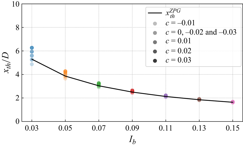
The near-wake length  $x_{th}^i$ is modelled according to Bastankhah & Porté-Agel (Reference Bastankhah and Porté-Agel2016) and Carbajo Fuertes, Markfort & Porté-Agel (Reference Carbajo Fuertes, Markfort and Porté-Agel2018) under the ZPG condition. Although it has been shown that pressure gradient influences the near-wake length to some extent, the sensitivity analysis presented in Appendix B.2 shows that using the model under the ZPG condition only leads to negligible differences in the calculation of
 $x_{th}^i$ in comparison with the model proposed by Dar et al. (Reference Dar, Gertler and Porté-Agel2023). Hence, we use the model under the ZPG condition for its low computational cost and simplicity of implementation.
The inflow turbulence intensity  $I_u^i$ is modelled as
 $\sqrt {I_b^2+ (\Delta I_u^i)^2 }$, where
 $I_b$ is the ambient streamwise turbulence intensity and
 $\Delta I_u^i$ is the added streamwise turbulence intensity at the rotor plane for
 $WT_i$, which may be induced by multiple wind-turbine wakes similar to the velocity deficit. Here we define the added turbulence intensity induced by
 $WT_j$ at the rotor plane of
 $WT_i$ as
 $\delta I_u^{j\rightarrow i}$, which can be calculated by the three-dimensional Gaussian model proposed by Ishihara & Qian (Reference Ishihara and Qian2018). To calculate
 $\Delta I_u^i$ in the merged wake region, we resort to the maximum superposition method expressed as
 $\Delta I_u^i=\max _{j=1}^{i-1}\delta I_u^{j\rightarrow i}$ (Niayifar & Porté-Agel Reference Niayifar and Porté-Agel2016), for more details about the superposition of the turbulence intensity, please refer to Li et al. (Reference Li, Wang, Ge, Huang, Li and Liu2023). It is noteworthy that the added turbulence intensity model is under the ZPG condition, which is also adopted by Dar & Porté-Agel (Reference Dar and Porté-Agel2024). Although pressure gradient may influence the production of turbulence intensity, developing such a model needs further research.
After obtaining the maximum velocity deficit  $C_0^i(x)$ and wake width
 $\sigma _0^i (x)$ under the ZPG condition,
 $\lambda _0^i(x)$ can be obtained by (2.21). Substituting
 $\lambda _0^i(x)$ into (2.20), it is easy to know that
 \begin{equation} \sigma^i(x)=\sigma_0^i(x)\left(\frac{u_0^i}{u_b^i(x)}\right)^{2/3}. \end{equation}
As shown by (2.20) and (2.24),  $C^i(x)$ and
 $\sigma ^i(x)$ can be expressed directly by its counterpart under the ZPG condition and the base flow variation. Under the FPG condition,
 $u_0^i$ will be less than
 $u_b^i(x)$, so both
 $C^i(x)$ and
 $\sigma ^i(x)$ will lower than its counterpart under the ZPG condition, indicating a faster wake recovery, and vice versa under the APG condition. By substituting these two variables into (2.13) and (2.14), the wake velocity deficit and wake velocity under pressure gradient can be obtained.
2.3. A simplified form of PG-IMCM
Based on the previous two subsections, we have presented the complete form and implementation details of the PG-IMCM method, which is summarised in Appendix A. What makes the PG-IMCM method difficult to implement and time-consuming to calculate is that the last two terms in (2.19) are integral quantities. Therefore, it is of practical interest for us to investigate the magnitude of these terms and to see whether they can be simplified. For instance, if the sum of the last two terms is small enough compared with  $U_{s,LWS}$, they can be neglected, resulting in a much simpler and computationally effective form. However, it is difficult for us to prove the assumption theoretically. Therefore, we first make a simple order-of-magnitude analysis of the sum of the last two terms in (2.19), which can be rewritten as
 \begin{equation} \Delta U_p=U_{s,{\mathfrak p}}-U_{s,{\mathfrak P}}=\frac{\sum_{i\in B} {\mathfrak p}^i-{\mathfrak P}}{U_c(x)}=\frac{1}{U_c(x)}\int_{x_0}^{x}\frac{{\rm d}U_b(x^\prime)}{{{\rm d}\kern0.7pt x}^\prime}\left(\sum_{i\in B} u_s^i-U_s\right) {{\rm d}\kern0.7pt x}^\prime, \end{equation}
where  $\sum _{i\in B} u_s^i$ represents the sum of individual velocity deficits using the local linear superposition method. In fact, the term in parentheses is the difference between the local linear superposition method and the PG-IMCM method, which is denoted as
 $\Delta U_s$. By definition, it is easy to know that the combined convective velocity
 $U_c(x)$ has the same order as the base flow
 $U_b(x)$. If we assume that the base flow has a linear speed-up ratio
 $\gamma$, i.e.
 ${\rm d}U_b/{{\rm d}\kern0.7pt x}=\gamma$, we can obtain
 \begin{equation} \Delta U_p\sim\frac{\gamma (x-x_0)}{U_b(x)}\underbrace{\frac{1}{x-x_0}\int_{x_0}^x \Delta U_s \,{{\rm d}\kern0.7pt x}^\prime}_{\overline{\Delta U_s}}, \end{equation}
where  $\overline {\Delta U_s}$ is the streamwise-averaged
 $\Delta U_s$. In general, the wind speed variation
 $\gamma (x-x_0)$ within the wind farm caused by pressure gradient has the same order as the base flow
 $U_b(x)$. Therefore,
 $\Delta U_p\sim \overline {\Delta U_s}$. Although it has been shown that
 $\overline {\Delta U_s}\approx 0$ under the ZPG condition (Zong & Porté-Agel Reference Zong and Porté-Agel2020), there is no generalised magnitude estimation applicable to FPG and APG conditions. Consequently, it is infeasible for us to analyse the magnitude of
 $\Delta U_p$ directly. Moreover, it is incomplete that we only know the magnitude of
 $\Delta U_p$ since whether we can neglect it depends on its relative magnitude to
 $U_{s,LWS}$. To this end, we further resort to a model sensitivity analysis under different wind-farm configurations and atmospheric states, which are typical of wind farm operational conditions under pressure gradient, as presented in table 1.
Case set-up for the sensitivity study of the PG-IMCM method.

Specifically, we consider the aligned wind farm layout and all wind turbines have the same thrust coefficient  $C_T=0.8$. The base flow is modelled as a piecewise function:
 \begin{equation}
U_b(x)=\begin{cases} U_{b0}[1+c(x-x_1)/D],\quad c\geq0,\\
U_{b0}[5+c(x-x_1)/D],\quad c<0, \end{cases}
\end{equation}
where  $x_1$ is the streamwise location of the first wind turbine,
 $U_{b0}$ is the inflow velocity at
 $x_1$ and
 $c=\gamma D/U_{b0}$ is the normalised speed-up ratio. When
 $c<0$, the inflow velocity is set to
 $5U_{b0}$ to prevent
 $U_{b}(x)<0$ at farther downstream, which is unphysical. By systematically varying the number of wind turbines
 $N$, streamwise spacing
 $S_x$, normalised speed-up ratio
 $c$ and ambient turbulence intensity
 $I_b$, the mean relative percentage of (2.25) to
 $U_{s,LWS}$ is quantified, which is defined as the streamwise-averaged absolute ratio of (2.25) to
 $U_{s,LWS}$ at the wake centreline for each case:
 \begin{equation} MRP_p=\frac{100\,\%}{x_N+S_x-x_1}\int_{x_1}^{x_N+S_x}\frac{|\Delta U_p|}{U_{s,LWS}}\,{{\rm d}\kern0.7pt x}, \end{equation}
where  $x_N$ is the streamwise location of the last wind turbine.
Overall, the averaged  $\overline {MRP}_p$ for all the cases is only about 0.4 %, indicating that neglect of the last two terms in the complete form will only lead to negligible error. Moreover, this implies that the local linear superposition method under pressure gradient has a very similar performance to the PG-IMCM method, as discussed later in § 5.2. Based on this analysis, we can provide a simplified form of PG-IMCM as follows:
 \begin{equation} \text{PG-IMCM-S:}\quad U_s(x,y,z)\approx\sum_{i\in B}\frac{u_c^i(x)}{U_c(x)}u_s^i(x,y,z). \end{equation}
As a simplified form of PG-IMCM, we denote it as PG-IMCM-S, and its calculation procedure is very similar to the PG-IMCM method, which is also given in Appendix A. It should be noted that PG-IMCM-S has the same form as Zong & Porté-Agel (Reference Zong and Porté-Agel2020), but the single turbine wake quantities  $u_c^i(x)$ and
 $u_s^i(x)$ are redefined to account for the influence of pressure gradient, as detailed in § 2.1.3. For the first time, our derivation and analysis reveal the similarities and differences between the momentum-conserving wake superposition methods under different pressure gradient conditions and form the basis for a unified framework. On the other hand, based on the form of PG-IMCM-S, it is demonstrated that wake superposition under pressure gradient does not need to explicitly account for the effect of pressure gradient, whereas it is necessary to account for the influence of pressure gradient on background wind speed and wake recovery when calculating individual velocity deficits. These implications pave the way for extending the empirical superposition principles under pressure gradient in § 5.
Although PG-IMCM and PG-IMCM-S have very close prediction results, their physical meanings differ significantly. PG-IMCM is the direct consequence by linearising the integral momentum-conserving equation, which has a solid theoretical foundation. Specifically, the integral of the product of the wind-farm convection velocity with the sum of the first two terms on the right-hand side of (2.19) is the total thrust of the wind farm, whereas the other term represents the influence of background pressure gradient. In contrast, PG-IMCM-S has limited physical insights and is only an indirect result of the momentum conservation equation. One advantage of the PG-IMCM-S method is that it is easy to implement and computationally effective.
The inputs of the model consist of environment variables and wind turbine variables. The former includes the base flow  $U_b(x)$ and ambient streamwise turbulence intensity
 $I_b$, whereas the latter consists of the rotor centre coordinates
 $(x_i,y_i,z_i)$, thrust coefficient
 $C_T^i$ and rotor diameter
 $D$ of
 $WT_i$. The output of the model is the wind-farm velocity deficit
 $U_s(x,y,z)$. In this study,
 $U_b$ is extracted directly from the main computational domain without wind turbines. For the wind farm layout optimisation in complex terrain, the background flow field can be modelled by using some computational fluid dynamics (CFD) tools, such as WAsP and WindSim, for a number of inflow wind direction sectors (Brogna et al. Reference Brogna, Feng, Sørensen, Shen and Porté-Agel2020). In addition, it can be modelled through some empirical functions (Sun, Yang & Gao Reference Sun, Yang and Gao2023) or linearised perturbation equations (Hunt, Leibovich & Richards Reference Hunt, Leibovich and Richards1988; Shamsoddin & Porté-Agel Reference Shamsoddin and Porté-Agel2018b) under some simple terrains (such as ramps and hills with gentle slopes).
3. LES methodology and case set-up
In this study, we use LES to simulate the evolution of wind-turbine wakes under different pressure gradients, which is used to compare and validate the performance of the proposed WFFAMs. Pressure gradient is simulated by complex terrains, which are modelled via the wall-modelled immersed boundary method (IBM). LES methodology and the validation case set-up are given below.
3.1. LES methodology
Here, we utilise the pseudo-spectral solver LESGO for numerical simulation, which has been validated by wind tunnel experiments (e.g. Stevens, Martínez-Tossas & Meneveau Reference Stevens, Martínez-Tossas and Meneveau2018; Liu & Stevens Reference Liu and Stevens2020b; Zhang et al. Reference Zhang, Huang, Bitsuamlak and Cao2022b) and widely adopted in the studies on wind turbines and wind-farm flows (Du et al. Reference Du, Ge, Zeng, Cui and Liu2021; Ge et al. Reference Ge, Yang, Zhang and Zuo2021; Ma et al. Reference Ma, Ge, Wu, Du and Liu2021; Zhang et al. Reference Zhang, Ge, Liu and Yang2021a; Du, Ge & Liu Reference Du, Ge and Liu2022, among others), atmospheric boundary layer over complex terrain (Liu & Stevens Reference Liu and Stevens2020a,Reference Liu and Stevensb; Zhang et al. Reference Zhang, Huang, Bitsuamlak and Cao2022b) as well as urban canopy flows (e.g. Ge et al. Reference Ge, Zhang, Meng and Ma2020; Fan et al. Reference Fan, Ge, Tan and Li2021; Ge et al. Reference Ge, Yang, Zhang and Zuo2021; Zhang et al. Reference Zhang, Ge, Liu and Yang2021a,Reference Zhang, Yang, Du and Geb, Reference Zhang, Du, Ge and Zuo2022a). LES solves the spatially filtered unsteady incompressible Navier–Stokes equations, where the continuity and momentum equations are written as
 $$\begin{gather} \frac{\partial \tilde{u}_{i}}{\partial x_{i}} = 0, \end{gather}$$
 $$\begin{gather}\frac{\partial \tilde{u}_{i}}{\partial t}+\tilde{u}_{j}\frac{\partial \tilde{u}_{i}}{\partial x_{j}} ={-}\frac{\partial \tilde{p}^{*}}{\partial x_{i}}-\frac{\partial \tau^{d}_{ij}}{\partial x_{j}}-\frac{f}{\rho}. \end{gather}$$
Here,  $\tilde {{\cdot }}$ is the filter at the spatial scale
 $\Delta$,
 $t$ is time,
 $\tilde {u}_i$ is the filtered velocity in the
 $i$-direction (with
 $i=1$, 2 and 3 corresponding to the streamwise (
 $x$), spanwise (
 $y$) and vertical (
 $z$) directions, respectively),
 $\tilde {p}^*=\tilde {p}/\rho +1/3\tau _{kk}$ is the modified pressure and
 $\tau _{ij}^d$ is the deviatoric part of the sub-grid scale stress tensor, which is modelled by the Smagorinsky model with wall damping function (Bou-Zeid, Meneveau & Parlange Reference Bou-Zeid, Meneveau and Parlange2005). Since the Reynolds number based on the rated wind speed (
 $\sim$10 m s
 $^{-1}$) and rotor diameter (
 $\sim$100 m) is
 ${\sim }10^7$, the effect of the viscous term in the momentum equation is neglected. Here
 $f$ is the external force, and it can originate from different sources as follows:
 \begin{equation} f=f_{p}+f_{t}-f_{IB}, \end{equation}
where  $f_{p}$ is the constant pressure gradient that drives the flow,
 $f_{t}$ represents the actuator force induced by the wind turbine and
 $f_{IB}$ is the body force that needs to be enforced to ensure the grid velocity is zero in the solid region.
Here, we adopt the wall-modelled IBM developed by Liu & Stevens (Reference Liu and Stevens2020b), which is a simplified version of the three-step level-set method proposed by Chester, Meneveau & Parlange (Reference Chester, Meneveau and Parlange2007). This method introduces a signed distance function  $\phi (\boldsymbol{x})$, and the computational domain is divided into solid region, fluid region and fluid–solid interface region based on
 $\phi (\boldsymbol{x})$ at first. Then, different treatments are used for different regions; that is, the velocity at the grid of the solid region is enforced to zero, and the sub-grid scale stress of the fluid–solid interface region is calculated using the wall model, whereas no further treatment is done to the grid in the fluid region. For more details about the wall-modelled IBM, please refer to Liu & Stevens (Reference Liu and Stevens2020b).
Wind turbines are modelled using the filtered actuator disk model (Shapiro, Gayme & Meneveau Reference Shapiro, Gayme and Meneveau2019). Based on the one-dimensional momentum theory, the total thrust  $F_t$ can be expressed as
 \begin{equation} F_t=\frac{1}{2}\rho AC_TU_{\infty}^2=\frac{1}{2}\rho AC_T\frac{U_d^2}{(1-a)^2}, \end{equation}
where  $U_{\infty }$ is the freestream inflow wind speed,
 $A$ is the swept area of the wind rotor,
 $\rho$ is the air density,
 $C_T$ is the thrust coefficient,
 $a$ is the axial induction factor and
 $U_d$ is the rotor-averaged velocity. Finally, the total thrust
 $F_t$ is distributed to the computation grids to obtain
 $f_{t}$ according to the Gaussian-filtered indicator function
 $\Re (\boldsymbol {x})$. For more details about the determination of
 $\Re (\boldsymbol {x})$, please refer to Shapiro et al. (Reference Shapiro, Gayme and Meneveau2019).
Uniform grids are used in the horizontal direction, and a staggered Cartesian grid is used in the vertical direction. The pseudo-spectral method is used for the horizontal spatial discretisation. In the vertical direction, the second-order central finite difference method is adopted. For time advancement, the code uses the second-order accurate Adams–Bashforth method.
Note that the filter symbol is omitted hereafter for convenience. Although the pressure simulated in this study includes the trace of the sub-grid scale stress tensor, it is expected only to cause a small difference in the momentum balance and the Bernoulli equation (Bastankhah et al. Reference Bastankhah, Welch, Martínez-Tossas, King and Fleming2021).
3.2. Case set-up
In general, convex (concave) topography will induce FPG (APG). To validate the performance of the proposed WFFAMs under pressure gradient, we set up two types of cases. One type is the ideal convex and concave channels consisting of symmetric upper and lower walls with respect to the centre plane of the channel (Shamsoddin & Porté-Agel Reference Shamsoddin and Porté-Agel2018a), which can be used to simulate FPG and APG conditions, respectively. The surface equation  $Z_l(x,y)$ of the lower wall has the following general cosine form:
 \begin{equation}
Z_l(x,y)=\begin{cases}
\displaystyle\frac{1}{2}H\left[1+\cos\left(\frac{\rm \pi}{2L_u}(x-x_{ct})\right)\right],
& -2L_u\leq x-x_{ct}<0,\\
\displaystyle\frac{1}{2}H\left[1+\cos\left(\frac{\rm \pi}{2L_d}(x-x_{ct})\right)\right],
& 0\leq x-x_{ct}<2L_d,\\ 0, & \text{otherwise}, \end{cases}
\end{equation}
where  $x_{ct}$ is the position of the channel throat,
 $H$ is the height difference between the throat position and the horizontal ground, and
 $L_u$ and
 $L_d$ are the upstream and downstream half-lengths of the cosine functions, respectively. The corresponding expression for the upper wall is
 $Z_u (x,y)=10D-Z_l(x,y)$. The detailed parameter settings are listed in table 2. In this condition, wind turbines are placed at the centre of the
 $y$–
 $z$ plane of the computational domain, as shown in figure 4.
Overview of the ideal convex and concave channel cases. (CVW and CCW represent the convex and concave walls, respectively, and WT represents there are wind turbines in this case;  $x_T$ is the streamwise location of the rotor centre.)

Schematics of the computational domain for (a) FPG-CVW-WT and (b) APG-CCW-WT.

Another type of case consists of two linear ramps and one platform at the bottom (Dar et al. Reference Dar, Gertler and Porté-Agel2023; Dar & Porté-Agel Reference Dar and Porté-Agel2024), as shown in figure 5. Wind turbines are placed at the same distance over the ground, and their rotors are perpendicular to the ramp. The hub height is the same as the rotor diameter. To facilitate the comparison between the proposed model and the ramp case, we define a local ramp coordinate following the slope of the ramp, whose origin is located in the rotor centre of the first wind turbine in the wind farm array, as shown in figure 5. This case setting is closer to the realistic engineering situation than channel cases. The analytical expression of the ramp height  $Z_r(x,y)$ is written as follows:
 \begin{align}
Z_r(x,y)=\begin{cases} H_r\left(\dfrac{x-x_w}{L_1}\right),
& x_w\leq x< x_w+L_1,\\ H_r, & x_w+L_1\leq x<
x_w+L_1+L_2,\\
H_r\left(1-\dfrac{x-x_w-L_1-L_2}{L_3}\right), &
x_w+L_1+L_2\leq x< x_w+L_1+L_2+L_3,\\ 0, &
\text{otherwise}, \end{cases}
\end{align}
where  $x_{w}$ is the starting location of the windward ramp,
 $H_r$ is the height of the platform,
 $L_2$ is the length of the platform, and
 $L_1$ and
 $L_3$ are the projected lengths of the windward and leeward ramps, respectively. The detailed parameter settings are given in table 3.
Schematics of the computational domain for (a) FPG-RAMP-WT and (b) APG-RAMP-WT.

Overview of the ramp cases.

It should be noted that although we made no assumptions about the wind-farm layout in the model derivation, we only simulated the aligned layout in the validation cases, which serves as a basis for verifying the wake superposition method (Zong & Porté-Agel Reference Zong and Porté-Agel2020; Lanzilao & Meyers Reference Lanzilao and Meyers2022; Dar & Porté-Agel Reference Dar and Porté-Agel2024). In this case, the wake generated by different wind turbines will be fully merged, and the wake superposition is very complicated, providing a fair condition to test the performance of different superposition methods.
The main computational domain for the FPG-CVW-WT, FPG-RAMP-WT and APG-RAMP-WT cases is set to  $80D\times 12D\times 10D$. However, due to the setting of concave walls, the main computational domain for the APG-CCW-WT case is expanded to
 $80D\times 12D\times 17D$. The number of grids in both computational domains is
 $320\times 120\times 144$, which can ensure the rotor diameter is covered with about 10 points in both the spanwise and vertical directions. Such a grid resolution is fine enough for the actuator disk model to predict the velocity deficit in turbine wakes with reasonable accuracy (Wu & Porté-Agel Reference Wu and Porté-Agel2011; Shamsoddin & Porté-Agel Reference Shamsoddin and Porté-Agel2018a,Reference Shamsoddin and Porté-Agelb; Lin & Porté-Agel Reference Lin and Porté-Agel2022). The thrust coefficient of all wind turbines is set to 0.8. In addition to the above four cases with wind turbines, four cases without wind turbines under the same condition are simulated in tables 2 and 3 to obtain the base flow, which is used as inputs to WFFAMs and to calculate the normalised velocity deficit. To overcome the streamwise periodicity and ensure a fully developed inflow to the main computational domain, we use the concurrent precursor method proposed by Stevens, Graham & Meneveau (Reference Stevens, Graham and Meneveau2014), in which the flow field in the fringe region at the end of the main domain is blended with the ideal straight channel flow for the curved channel cases and half-channel flow for the ramp cases, whose domain size and grid size are the same as the main computational domain. The computational accuracy of the LES framework in these channel and half-channel flows has been tested in several validation studies (e.g. Shamsoddin & Porté-Agel Reference Shamsoddin and Porté-Agel2018a,Reference Shamsoddin and Porté-Agelb; Liu & Stevens Reference Liu and Stevens2020b; Zhang et al. Reference Zhang, Huang, Bitsuamlak and Cao2022b). The surface roughness of the ground and topography are both
 $0.001D$, a typical value of onshore topography.
4. Model validation
In this section, we compare the prediction accuracy of PG-IMCM and its simplified form based on LES results. To make a more straightforward comparison, we compute the normalised velocity deficit as follows:
 \begin{equation} \frac{U_s(x,y,z)}{U_{b0}}=\frac{U_{bg}(x,y,z)-U_{w}(x,y,z)}{U_{b0}}, \end{equation}
where  $U_{bg}$ and
 $U_{w}$ are the time-averaged background flow velocity and wind-farm flow velocity, respectively, and
 $U_{b0}$ is the hub-height spanwise-averaged
 $\langle U_{bg}\rangle _y$ at the streamwise location of the first wind turbine for each validation case. The model input
 $U_b(x)$ is the hub-height spanwise-averaged
 $\langle U_{bg}\rangle _y$.
4.1. Validation of the momentum-conserving method under FPG
In this subsection, we validate the performance of the momentum-conserving method under FPG. Under FPG condition, the pressure decreases streamwise, and the background wind velocity increases, which is beneficial to the wake recovery (Shamsoddin & Porté-Agel Reference Shamsoddin and Porté-Agel2018a).
4.1.1. Validation of results based on the FPG-CVW-WT case
Figure 6(a) shows the streamwise variations of the normalised spanwise-averaged velocity and pressure at hub height for the FPG-CVW case. It can be seen that the pressure decreases as the streamwise distance increases, and the wind speed increases gradually, indicating that we have successfully simulated the ideal FPG case. The mean base flow gradient  $\overline {{\rm d}U_b/{{\rm d}\kern0.7pt x}}$ from
 $16D$ to
 $50D$ is about
 $0.0224U_{b0}/D$. In addition, figure 6(b) shows the streamwise variations of the normalised spanwise-averaged kinetic energy gradient and pressure gradient at hub height for the FPG-CVW case. We can see that these two curves nearly coincide, indicating that the pressure and wind speed satisfy the Bernoulli equation
 $\langle P_{bg}\rangle _y/\rho +1/2 \langle U_{bg} \rangle _y^2=\text {const.}$. Therefore, this case meets the applicability of the wake model and PG-IMCM superposition method under pressure gradient, which is necessary for a fair comparison.
Streamwise variations of the normalised spanwise-averaged (a) velocity and pressure and (b) kinetic energy gradient and pressure gradient at hub height for the FPG-CVW case. (Vertical black dashed lines represent the locations of wind turbines.)

Figure 7 presents the contours of the normalised velocity deficit at the  $x$–
 $z$ rotor symmetry plane. It can be seen that the velocity deficit downstream of the first wind turbine is the smallest, and its recovery is the slowest, whereas the wake velocity deficit downstream of the last wind turbine is the largest. In addition, the second and third wind turbines have similar wake velocity deficit and recovery rates.
Contours of the normalised velocity deficit at the  $x$–
 $z$ rotor symmetry plane for the FPG-CVW-WT case.

Whether the maximum velocity deficit at hub height  $U_{s,max}$ in the merged wake region can be accurately predicted is one of the crucial metrics for the assessment of superposition methods. Figure 8 shows the comparison of
 $U_{s,max}/U_{b0}$ obtained by PG-IMCM and LES for the FPG-CVW-WT case. In addition to the total velocity deficit, its decomposition terms (i.e.
 $U_{s,LWS}$,
 $U_{s,{\mathfrak p}}$ and
 $-U_{s,{\mathfrak P}}$) are also presented in the figure. As expected, the sum of the pressure correction term induced by individual velocity deficits
 $\sum _{i\in B} {\mathfrak p}^i$ and the pressure correction term induced by total velocity deficit
 $-{\mathfrak P}$ accumulate with the downstream distance, as they are integral quantities. When divided by the combined velocity
 $U_c$, they become
 $U_{s,{\mathfrak p}}$ and
 $-U_{s,{\mathfrak P}}$, whose variation is very similar to the sum of four stair-step functions located at the wind-turbine locations. As expected, they have opposite symbols but very close magnitudes, and the mean absolute value of their sum is only about
 $0.008U_{b0}$. Therefore, the sum of these two terms can be neglected, and the prediction result of the PG-IMCM method can be viewed as the linear-weighted sum of individual velocity deficits. In addition, we also present the prediction results of PG-IMCM-S, which is virtually identical with PG-IMCM, further validating our simplification based on the sensitivity study. Overall, PG-IMCM and its simplified form have a good prediction over
 $U_{s,max}$, only with a slight overestimation in the merged wake region.
Model prediction of  $U_{s,max}/U_{b0}$ in comparison with LES for the FPG-CVW-WT case. (Vertical black dashed lines represent the locations of wind turbines.)

Furthermore, we are also concerned about the prediction of velocity deficit profiles by WFFAMs in practical applications since it is closely related to the power calculation of wind turbines. Figure 9 compares the spanwise velocity deficit profiles at hub height obtained by PG-IMCM, PG-IMCM-S and LES downstream of each wind turbine for the FPG-CVW-WT case. Similar to figure 8, a term-by-term comparison is also presented. At first, we can see that  $U_{s,{\mathfrak p}}$ and
 $-U_{s,{\mathfrak P}}$ have a near Gaussian distribution, and their sum can be neglected. The prediction of PG-IMCM and its simplified form is nearly collapsed at each radial location, similar to the rotor centre. Overall, the PG-IMCM method and its simplified form have a good prediction accuracy over the profiles, with a slight overestimation in the rotor centre region.
Model prediction of the spanwise velocity-deficit profiles at hub height downstream of each wind turbine in comparison with LES for the FPG-CVW-WT case.

LES results can not only serve as a baseline for the model validation but also can be used to examine some assumptions in the derivation of the PG-IMCM method. Here, we compare the wind turbine thrust modelling (2.16) based on the single-wake quantities with LES results, as shown in figure 10. It can be seen that the wind thrust modelling can represent the variation and magnitude of the total thrust in the control volume  $B$ very well. The sum of momentum deficits of stand-alone turbine wakes
 $\sum _{i\in B} T_{MD}^i$ under FPG condition is less than the total thrust, whereas the sum of pressure correction terms
 $\sum _{i\in B} T_{{\mathfrak p}}^i$ makes up for this deficit, finally resulting in a good prediction of the total thrust, which is an essential part of the PG-IMCM method. It should be noted that the slight underestimation in the near-wake region is related to the modified thrust coefficient within the downstream
 $2D$ region.
Comparison of the modelled wind-turbine thrust with LES for the FPG-CVW-WT case. (Vertical black dashed lines represent the locations of wind turbines.)

4.1.2. Validation of results based on the FPG-RAMP-WT case
The FPG-CVW-WT case is too ideal, leading to minimal wind shear and ambient streamwise turbulence intensity (about 2.3 %) in the rotor region, which does not represent the realistic atmospheric surface boundary layer with high wind shear and high turbulence intensity. Therefore, to further validate the applicability of the proposed momentum-conserving method under FPG condition, we set up the FPG-RAMP-WT case, as depicted in figure 5(a), which is closer to the realistic operation environment of the wind turbine. In this case, streamwise turbulence intensity at hub height is about 6 %. Because of the ramp, the flow has a streamwise component  $U_x$ and a vertical component
 $U_z$. Therefore, the velocity
 $U$ used in the analysis of the FPG-RAMP-WT and APG-RAMP-WT cases is
 $\sqrt {U_x^2+U_z^2}$.
Figure 11 shows the contours of the spanwise-averaged wind field and pressure for the FPG-RAMP case. It can be observed that the flow up the windward ramp evolves downstream approximately parallel to the surface and gradually accelerates before approaching the platform. The corresponding pressure gradually decreases, indicating that the FPG condition is successfully simulated through this set-up. The base flow has a nearly constant speed-up ratio above the windward ramp, and its mean value  $\overline {{\rm d}U_b/{\rm d}{\kern0.8pt}x_r}$ from
 $0D$ to
 $26D$ is about
 $0.0215U_{b0}/D$. We also examined the kinetic energy gradient and pressure gradient at hub height for the FPG-RAMP case, and they still approximately conform to the Bernoulli equation. Here, we do not show them for brevity.
Contours of the spanwise-averaged (a) wind field and (b) pressure for the FPG-RAMP case. (The white dashed line represents hub height, and black solid lines represent streamlines.)

Figure 12 shows the contours of the normalised velocity deficit and streamwise turbulence intensity at the  $x$–
 $z$ rotor symmetry plane for the FPG-RAMP-WT case. We can see that the velocity deficit computed by LES has an obvious accumulation pattern in this case; that is, the wake velocity deficit of the first wind turbine is the smallest, whereas the wake velocity deficit downstream of the third wind turbine is the largest. As for the streamwise turbulence intensity, its magnitude in the wake of the first wind turbine is low, whereas its magnitude downstream of the second and third wind turbines is high, and their spatial distribution is quite similar. This finding is consistent with Li et al. (Reference Li, Wang, Ge, Huang, Li and Liu2023), who have studied the spatial distribution characteristics of the added streamwise turbulence intensity in the merged wake region of an aligned wind turbine array under the ZPG condition, indicating that the adoption of the maximum superposition method for the wake-added turbulence is reasonable.
Contours of the (a) normalised velocity deficit and (b) streamwise turbulence intensity at the  $x$–
 $z$ rotor symmetry plane for the FPG-RAMP-WT case. (The white dashed line represents hub height.)

Figures 13 and 14 show the comparison of  $U_{s,max}/U_{b0}$ and the spanwise velocity deficit profiles at hub height obtained by the momentum-conserving WFFAMs and LES for the FPG-RAMP-WT case, respectively. The term-by-term comparison results are very similar to the FPG-CCW-WT case, thus not repeated here. Overall, the momentum-conserving methods show a remarkably high prediction accuracy in this case, further validating the accuracy of the proposed superposition method. A comparison of the modelled turbine thrust with LES results is further shown in figure 15. Similar to the results presented in figure 10, we can observe that the modelled turbine thrust agrees well with LES results, further confirming the validity of (2.16).
Same as figure 8, but for the FPG-RAMP-WT case.

Same as figure 9, but for the FPG-RAMP-WT case.

Same as figure 10, but for the FPG-RAMP-WT case.

The term-by-term analysis of the proposed momentum-conserving method in the above two cases with different ambient turbulence intensity under FPG conditions confirms the validity of the linearised expression of the turbine thrust derived in § 2.1.3 and shows that our proposed model can predict the maximum velocity deficit and spanwise velocity deficit profiles at hub height very well.
Interestingly, the proposed methods have higher accuracy in the realistic ramp case than the ideal concave channel case. This may be attributed to two reasons. On the one hand, the ambient streamwise turbulence intensity is only 2.3 % in the ideal concave channel case, resulting in a much longer near-wake region. The velocity deficit profiles of the first turbine are closer to super-Gaussian, as depicted in figure 9(a). When we use the Gaussian profile, it will result in a more slender spanwise profile. On the other hand, the ideal curved channel cases may be out of the application range of some empirical relation of wake quantities, especially the wake growth rate. This is because this expression is obtained by curve-fitting based on the LES results and field measurements in the atmospheric boundary layer, which is characterised by the high wind shear and ambient turbulence intensity.
4.2. Validation of the momentum-conserving method under APG
In this subsection, we focus on the validation of the momentum-conserving method under APG. In contrast to the FPG condition, the pressure increases streamwise and the corresponding wind velocity decreases under the APG condition. Compared with the ZPG condition, the APG condition will make the wake recovery slower (Shamsoddin & Porté-Agel Reference Shamsoddin and Porté-Agel2018a).
4.2.1. Validation of results based on the APG-CCW-WT case
The base flow has a nearly constant gradient in the region of interest, and the mean base flow gradient  $\overline {{\rm d}U_b/{{\rm d}\kern0.7pt x}}$ from
 $16D$ to
 $50D$ is about
 $-0.0062U_{b0}/D$ for the APG-CCW case. The ambient turbulence intensity is about 2.5 %. In addition, we compare the normalised spanwise-averaged kinetic energy gradient and pressure gradient at hub height for the APG-CCW case, and they almost collapse, indicating that the case set-up satisfies the applicability of the wake model and the PG-IMCM superposition method. For brevity, we do not show them here. Figure 16 shows the contours of the normalised velocity deficit at the
 $x$–
 $z$ rotor symmetry plane for the APG-CCW-WT case. It can be seen that the wake recovery is the slowest downstream of the first wind turbine. The wake velocity deficit downstream of the second wind turbine is the largest, and then it recovers very quickly. The wake velocity deficits and their recovery downstream of the third and fourth wind turbines are relatively similar. In this case, the spatial distribution of the merged wake velocity deficit is significantly different from that under ZPG and FPG conditions. The proposed momentum-conserving method cannot accurately predict the variations in the maximum velocity deficit in the merged wake region in this case, as shown in figure 17.
Same as figure 7, but for the APG-CCW-WT case.

Model prediction of  $U_{s,max}/U_{b0}$ in comparison with LES for the APG-CCW-WT case.

One possible explanation for this phenomenon is the combined effects of the low ambient turbulence intensity and APG, which stimulates the wake meandering behind the second wind turbine. Observations from various studies, such as Gupta & Wan (Reference Gupta and Wan2019), Li, Dong & Yang (Reference Li, Dong and Yang2022), Gambuzza & Ganapathisubramani (Reference Gambuzza and Ganapathisubramani2023) and Messmer, Hölling & Peinke (Reference Messmer, Hölling and Peinke2024), have supported the mechanism that wake meandering occurs in the far wake due to the amplification of upstream disturbances by shear flow instabilities, especially when the inflow's turbulence intensity is low. Moreover, the optimal perturbations are those large-scale (the same order as the turbine rotor) and low-frequency coherent eddies (Mao & Sørensen Reference Mao and Sørensen2018). This is the situation for the second wind turbine, which is immersed in the wake of the first wind turbine. In this condition, the small perturbations in the far-wake region of the first turbine will be amplified significantly by the complex nonlinear dynamics, leading to enhanced wake recovery. As a result, the wake downstream of the second wind turbine recovers quickly and is in an unsteady physical process, which does not satisfy the applicability of existing wake models and their empirical expressions. A similar phenomenon has also been observed in the study on the influence of swells on the wake evolution of aligned wind turbines (Yang et al. Reference Yang, Ge, Abkar and Yang2022).
Although the same situation is also satisfied in the FPG-CVW-WT case, our model only has a slight underestimation of wake recovery, which may be related to the potential influence of pressure gradient on the wake meandering. In other words, the FPG condition will suppress the selective amplification, making the empirical expression of wake growth rate still applicable only with a minor error, whereas the APG condition will enhance this process, resulting in a high prediction error.
It should be noted that our explanation is a qualitative conjecture based on the simulation results. A quantitative analysis on the influence of pressure gradient on wake meandering, especially the selective amplification mechanism, is beyond the scope of the study, which is an interesting topic for future research.
Therefore, the misestimation of PG-IMCM in this case can be attributed to the invalidity of the stand-alone turbine wake model rather than the superposition method. No further comparison based on this case is given hereafter for brevity.
4.2.2. Validation of results based on the APG-RAMP-WT case
To solve the problems mentioned previously, we further set up a leeward ramp to simulate the APG condition with a high ambient turbulence intensity, as depicted in figure 5(b). The prediction results of the momentum-conserving method in this case are further compared and analysed.
At first, figure 18 shows the contours of the spanwise-averaged wind field and pressure for the APG-RAMP case. We can observe that the flow upper the leeward ramp evolves downstream nearly parallel to the surface and gradually decelerates before approaching the ground, and the corresponding pressure gradually increases. It indicates that the expected APG condition is successfully simulated. The base flow has a nearly constant gradient above the leeward ramp, and its mean value  $\overline {{\rm d}U_b/{\rm d}{\kern0.8pt}x_r}$ from
 $0D$ to
 $26D$ is about
 $-0.0128U_{b0}/D$. Furthermore, we compare the kinetic energy gradient and pressure gradient at hub height for the APG-RAMP case. Similar to the FPG-RAMP case, they approximately satisfy the Bernoulli equation in the region of interest and meet the prerequisite of the wake model and the PG-IMCM superposition model under pressure gradient. For brevity, we do not show them here.
Same as figure 11, but for the APG-RAMP case.

The contours of the normalised velocity deficit and streamwise turbulence intensity at the  $x$–
 $z$ rotor symmetry plane for the APG-RAMP-WT case are depicted in figure 19. In the upper region of the leeward ramp, the downslope flow affects the wind turbine, and the streamwise turbulence intensity at the location of
 $WT_i$ is about 16 %. As a result, wind-turbine wakes recover very quickly. Figures 20 and 21 show the comparison of
 $U_{s,max}/U_{b0}$ and the spanwise velocity deficit profiles at hub height obtained by the momentum-conserving WFFAMs and LES for the APG-RAMP-WT case, respectively. Due to
 ${\rm d}U_b/{\rm d}{\kern0.8pt}x_r<0$ under APG condition,
 $U_{s,{\mathfrak p}}$ is less than zero, whereas
 $-U_{s,{\mathfrak P}}$ is larger than zero, which is in contrast to the case under the FPG condition. These two terms have a relatively close absolute value, with the mean absolute value of their sum only about
 $0.004U_{b0}$. Hence, neglecting them only leads to negligible differences throughout the region of interest. The momentum-conserving method performs well in this case, validating the applicability of PG-IMCM and its simplified form under APG condition.
Same as figure 12, but for the APG-RAMP-WT case.

Same as figure 8, but for the APG-RAMP-WT case.

Same as figure 9, but for the APG-RAMP-WT case.

Figure 22 compares the cumulative turbine thrust modelled by (2.16) with LES results in this case. Different from the FPG condition,  $\sum _{i\in B}T_{MD}^i$ under APG condition is larger than the thrust, whereas the pressure correction term
 $\sum _{i\in B} T_{\mathfrak p}^i$ cuts down this excess, finally leading to a satisfactory prediction of the cumulative turbine thrust.
Same as figure 10, but for the APG-RAMP-WT case.

In summary, the proposed model has a satisfactory performance in this APG condition. It is worth mentioning that the APG condition usually occurs in the high-turbulence leeward region in the atmospheric boundary layer, which is far from the ideal case studied in § 4.2.1. Therefore, although the PG-IMCM model has a poor performance in the ideal APG-CCW-WT case, which is related to the inapplicability of empirical expression for individual velocity deficits, it will not influence its engineering applications in realistic APG conditions similar to the APG-RAMP-WT case, in which it still has a high prediction accuracy.
5. Comparison with empirical superposition principles
Motivated by the simplified form PG-IMCM-S, which is free of the pressure correction term in the superposition method, it is of great interest to examine the applicability of some empirical superposition principles under pressure gradient. In § 5.1, we extend the empirical superposition methods mentioned in § 1.2 to account for the pressure gradient and compare their predictions with PG-IMCM and LES results in § 5.2.
5.1. WFFAMs under pressure gradient based on empirical superposition principles
Specifically, we can develop five empirical WFFAMs based on the empirical superposition methods (i.e. global linear, global square, local linear, local square and wind product) introduced in § 1.2 and the single-wake model under pressure gradient given in § 2.2. In addition, we have shown that these empirical WFFAMs may have a good performance provided that they can account for the base flow variations based on our derivation, which is also supported by Dar & Porté-Agel (Reference Dar and Porté-Agel2024). Therefore, their forms have been changed as follows:
 \begin{align} &\text{PG-GL:}\quad U_s(x,y,z)=\sum_i(U_b(x)-u_w^i(x,y,z)), \end{align}
 \begin{align} &\text{PG-GS:}\quad U_s(x,y,z)=\sqrt{\sum_i(U_b(x)-u_w^i(x,y,z))^2}, \end{align}
 \begin{align} &\text{PG-LL:}\quad U_s(x,y,z)=\sum_i( u_b^i(x)-u_w^i(x,y,z)), \end{align}
 \begin{align} &\text{PG-LS:}\quad U_s(x,y,z)=\sqrt{\sum_i( u_b^i(x)-u_w^i(x,y,z))^2}, \end{align}
 \begin{align} &\text{PG-WP:}\quad U_s(x,y,z)=U_b(x)-U_b(x)\prod_i\left(\frac{u_w^i(x,y,z)}{u_b^i(x)}\right). \end{align}
Compared with their counterparts under the ZPG condition, there are three main differences: (i)  $U_\infty$ is replaced by
 $U_b(x)$; (ii)
 $u_0^i$ is replaced by
 $u_b^i(x)$, which is the base flow for
 $WT_i$ defined in § 2.1.2; (iii) the calculation of
 $u_w^i(x,y,z)$ will account for the influence of pressure gradient. To be consistent with the different physical meanings between global and linear under the ZPG condition, the base flow and turbulence intensity used to calculate
 $u_w^i$ are different. In the global superposition methods (i.e. PG-GL and PG-GS),
 $u_w^i$ is calculated based on
 $U_b(x)$ and ambient turbulence intensity
 $I_b$, whereas
 $u_w^i$ is calculated based on
 $u_b^i(x)$ and inflow turbulence intensity
 $I_u^i$ in the local superposition methods (i.e. PG-LL and PG-LS) and PG-WP.
In total, we have developed five empirical WFFAMs under pressure gradient, and their classification and details are given in table 4. They have the same inputs and output as the momentum-conserving model. The step-by-step procedures of these empirical WFFAMs are detailed in Appendix C.
Classification and details of the proposed empirical WFFAMs under pressure gradient.

5.2. Validation results
In this subsection, we inter-compare the prediction results of these five empirical WFFAMs in the FPG-CVW-WT, FPG-RAMP-WT and APG-RAMP-WT cases. Figure 23 shows the comparison of the  $U_{s,max}/U_{b0}$ obtained by the empirical WFFAMs and PG-IMCM with LES for the three validation cases. We can see that the prediction of empirical WFFAMs under pressure gradient have many similarities with their counterparts under the ZPG condition. Overall, the PG-GL model will significantly overestimate the wind farm velocity deficit
 $U_s$ in the merged wake region. This is likely due to the fact that the background velocity, which does not account for the wake effect of upstream wind turbines, is used as the base flow, leading to the overestimation of individual wake velocity deficits. Moreover, when they are summed directly as the PG-GL model, it will overestimate
 $U_s$. If they are superimposed as the PG-GS model, it seems that only the largest individual wake velocity deficit will be left, and this may alleviate the overestimation of
 $U_s$. However, the PG-GS method still fails to have a satisfactory prediction, especially when the ambient turbulence intensity is low to moderate. If we use the base flow updated by accounting for upstream turbine wakes, the individual velocity deficits may be predicted accurately. However, when they are superimposed as the PG-LS model, it may suffer from the same problems as the PG-GS model, leading to the underestimation of the combined velocity deficit. Overall, the PG-LL model has a satisfactory performance. These findings are consistent with the inter-comparison results under the ZPG condition (Niayifar & Porté-Agel Reference Niayifar and Porté-Agel2016; Zong & Porté-Agel Reference Zong and Porté-Agel2020; Bastankhah et al. Reference Bastankhah, Welch, Martínez-Tossas, King and Fleming2021). In addition, the prediction results of the PG-WP model are almost identical to those of the PG-LL model, which is also observed by Lanzilao & Meyers (Reference Lanzilao and Meyers2022) under the ZPG condition.
Comparison of  $U_{s,max}/U_{b0}$ obtained by different WFFAMs with LES for the cases: (a) FPG-CVW-WT, (b) FPG-RAMP-WT and (c) APG-RAMP-WT. Vertical black dashed lines represent the locations of wind turbines.

Comparison of (a) the spanwise velocity deficit profiles at hub height and (b) vertical velocity deficit profiles at the  $x$–
 $z$ rotor symmetry plane obtained by different WFFAMs with LES downstream of each wind turbine for the FPG-CVW-WT case.

Comparison of (a) the spanwise velocity deficit profiles at hub height and (b) vertical velocity deficit profiles at the  $x_r$–
 $z_r$ rotor symmetry plane obtained by different WFFAMs with LES downstream of each wind turbine for the FPG-RAMP-WT case. Black dot-dashed lines represent the hub height.

Same as figure 25, but for the APG-RAMP-WT case.

Interestingly, the performance of PG-LL and PG-WP is very close to the momentum-conserving method, with only discernable differences in the near-wake region of the merged wake, which has also been observed in Zong & Porté-Agel (Reference Zong and Porté-Agel2020). This is related to the gradual variation of the mean convection velocity  $u_c$ and the sudden change in the combined convection velocity
 $U_c$ in the near-wake region of downstream turbines, leading to the weights for individual velocity deficits in these regions deviating from 1, which is exactly the weight of the PG-LL model. In contrast, the weight for individual velocity deficits in the PG-IMCM method in the far-wake region of downstream turbines will approach 1, resulting in a nearly collapsed prediction. A direct comparison between PG-WP and PG-IMCM is more intricate, as they have quite different forms. However, we believe that its high prediction accuracy lies in its intrinsic ability to update the base flow for downstream wind turbines, which is supported by Dar & Porté-Agel (Reference Dar and Porté-Agel2024).
Figures 24–26 further show comparisons of the spanwise and vertical velocity deficit profiles obtained by different WFFAMs against LES results for FPG-CVW-WT, FPG-RAMP-WT and APG-RAMP-WT case, respectively. Overall, the PG-IMCM, PG-LL and PG-WP models have the best performance. As expected, the spanwise and vertical profiles are almost identical in the convex channel case since it is free from the influence of the wall. In contrast, affected by the windward or leeward ramp, the wake velocity deficit has asymmetric characteristics. As a result, the spanwise and vertical wake widths have some differences, especially in the APG-RAMP-WT case. In addition, the wake centre position is slightly shifted downwards with respect to the hub height in the FPG-RAMP-WT case, as shown in figure 12(a), whereas the wake centre shifts upwards in the APG-RAMP-WT case, as depicted in figure 19(a). These pose significant challenges to accurately predicting the spatial distribution of wake velocity deficit and are difficult to model. Nevertheless, the adoption of the axisymmetric wake model and the same spanwise and vertical wake growth rates in the WFFAMs still have satisfactory performance, as shown in figures 25 and 26(b). The difference in the wake width prediction of the APG-RAMP-WT case can be alleviated to some extent by lowering the spanwise wake growth rate slightly and increasing the vertical wake growth rate accordingly to keep the equivalent wake width unchanged. However, developing a general empirical relationship of wake growth rates in different directions is beyond the scope of this study, and it needs to be better understood and addressed in future research.
Overall, the inter-comparison results of the empirical WFFAMs under pressure gradient share many similarities with the inter-comparison results under the ZPG condition. Among the five considered empirical models, the PG-LL and PG-WP models have a satisfactory and consistent performance with the PG-IMCM model in all validation cases, especially in realistic ramp cases. The secret behind their good performance can be attributed to the ability to properly update the base flow for the downstream wind turbines as well as reasonable superposition principles.
6. Conclusions
Pressure gradient over topography will significantly affect the wind-farm flow. To date, the wake superposition method and WFFAMs that account for its effect are unexplored, which significantly limits engineering applications such as wind farm wake loss evaluation and micro-site selection over complex terrain. To bridge this gap, we have theoretically derived an implicit momentum-conserving superposition method under pressure gradient (PG-IMCM). Based on the physical insights gained in the model derivation, we have further investigated the empirical superposition methods. In addition, we have systematically validated their performance based on LESs.
The PG-IMCM method has been derived based on the simplified integral RANS equation, which states that the total momentum deficit is equal to the sum of wind-turbine thrusts and the integral of pressure correction  ${\mathfrak P}$ induced by the wind-farm velocity deficit
 $U_s$. For an arbitrary wind turbine under pressure gradient, its thrust can be decomposed into the momentum deficit and the integral of pressure correction
 ${\mathfrak p}$ induced by its own velocity deficit
 $u_s$. The momentum deficit for the single turbine wake and the total momentum deficit under pressure gradient can be linearised by the mean convection velocity
 $u_c$ and the combined convection velocity
 $U_c$, respectively, which are introduced by Zong & Porté-Agel (Reference Zong and Porté-Agel2020). After linearisation, we can see that the wind-farm velocity deficit
 $U_s$ consists of the linear-weighted sum of individual wake velocity deficits, the sum of the pressure correction terms induced by individual wake velocity deficit divided by
 $U_c$, and pressure correction term induced by wind-farm velocity deficit divided by
 $U_c$.
Based on an order-of-magnitude and sensitivity study representing typical wind farm operational conditions, we can verify that the sum of the last two terms has a relatively small value, only about 0.4 % of the first term, and thus can be neglected, resulting in a simplified form PG-IMCM-S, which only includes the linear-weighted sum of individual wake velocity deficits. It is noteworthy that PG-IMCM-S has the same form as its counterpart under the ZPG condition, but with the single-wake quantities redefined based on the wake model under pressure gradient. Individual wake velocity deficit  $u_s$ is modelled as the asymptotic solution of the stand-alone wake model under pressure gradient, and the mean convection velocity
 $u_c$ is generalised to account for the influence of pressure gradient on the single-turbine wake evolution.
The proposed PG-IMCM model and its simplified form have been validated based on the ideal convex/concave channel cases and the realistic ramp cases simulated by LES with the wall-modelled IBM. The results show that our proposed model can accurately represent wind turbine thrust, validating some assumptions used to derive the model. PG-IMCM and its simplified form have virtually identical prediction results, and they can predict the maximum velocity deficit and spanwise velocity deficit profiles at hub height very well, except for the ideal concave channel. The overestimation of wind-farm velocity deficit for the ideal concave channel may be attributed to the inapplicability of empirical wake growth rate relation rather than the proposed superposition method. The above finding points out one limitation of the proposed method, that is, its accuracy is quite sensitive to the individual wake velocity deficit modelling, especially the wake growth rate, which is still an ongoing research topic. Nevertheless, the empirical relations used in our study can provide good prediction capability in the realistic ramp cases, which is of great significance to engineering applications.
Last but not least, we have developed five empirical superposition methods accounting for pressure gradient (i.e. PG-GL, PG-GS, PG-LL, PG-LS and PG-WP) based on the global linear, global square, local linear, local square and wind product superposition principles, respectively, which are well-defined under the ZPG condition. Their differences mainly lie in the adoption of the spatial-varying base flow and the calculation of individual wake velocity deficit. Further inter-comparison results have shown that PG-GL and PG-GS significantly overestimate the velocity deficit in the merged wake region, whereas PG-LS underestimates this quantity. PG-LL and PG-WP have the best performance, and they nearly collapse with the momentum-conserving method, with only discernable differences in the near-wake region of the merged wake. The high accuracy of these two empirical methods lies in their ability to properly update the base flow for downstream wind turbines and their superposition principles.
In summary, the PG-IMCM method and its simplified version perform relatively well in various validation cases, provided that the individual wake velocity deficits can be modelled accurately. They can be used to evaluate the influence of pressure gradient on wind-farm flows over complex terrain. In addition, PG-LL and PG-WP are two attractive empirical superposition methods, as they have comparable prediction accuracy but much lower computational cost in comparison with the momentum-conserving method.
Future research will focus on the validation of the proposed method under the partial-wake or deep-array condition, which is generally viewed as more challenging for the wake superposition method.
Acknowledgement
The authors thank the anonymous referees for their insightful comments and valuable feedback on the manuscript.
Funding
This research was supported by Beijing Natural Science Foundation (grant number JQ22008), the National Natural Science Foundation of China (grant number 12172128) and the State Key Laboratory for Alternative Electrical Power System with Renewable Energy Sources (grant number LAPS202201).
Declaration of interests
The authors report no conflict of interest.
Appendix A. Step-by-step procedure of the momentum-conserving WFFAM
From the perspective of code implementation, the PG-IMCM and PG-IMCM-S have a recursive cycle to update the base flow for downstream turbines one by one. Moreover, we employ an iteration method to ensure the convergence of the combined convection velocity  $U_c$ in each recursive step. The step-by-step procedure is as follows.
(1) Calculate the single-turbine wake quantities of
 $WT_i\ (1\leq i\leq N)$ under ZPG.
(1.1) Added turbulence intensity model of Ishihara & Qian (Reference Ishihara and Qian2018)
$\rightarrow \delta I_u^{j\rightarrow i}$.(1.2) Maximum added turbulence superposition model of Niayifar & Porté-Agel (Reference Niayifar and Porté-Agel2016)
$\rightarrow I_u^i$.(1.3) Wake growth rate model
$\rightarrow k_w^i$.(1.4) Near-wake length model
$\rightarrow x_{th}^i$.(1.5) Quasi-linear growth model for wake width
$\rightarrow \sigma _0^i(x)$.(1.6) Normalised maximum velocity deficit model under the ZPG condition
$\rightarrow C_0^i(x)$.
(2) Assume that there are
$n$ wind turbines with the initial value of $n=1$ and calculate the wind-farm velocity deficit $U_s^n$ for $n$ wind turbines.
(2.1) Calculate the stand-alone turbine wake quantities of
$WT_i$ ($1\leq i\leq n$) under pressure gradient.
(2.1.1) Normalised maximum velocity deficit under pressure gradient
$\rightarrow C^i(x)=C_0^i(x)[{u_b^i(x_i)}/{u_b^i(x)}]^{5/3}$.(2.1.2) Mean convection velocity model under pressure gradient
$\rightarrow u_c^i=u_b^i(x)(1-{C^i(x)}/{2})$.(2.1.3) Wake width under pressure gradient
$\rightarrow \sigma ^i(x)=\sigma _0^i(x)[{u_b^i(x_i)}/{u_b^i(x)}]^{2/3}$.(2.1.4) Wake velocity deficit under pressure gradient
$\rightarrow u_s^i(x,y,z)= u_b^i(x)C^i(x) \exp (-{[(y-y_i)^2+(z-z_i)^2]}/{2(\sigma ^i)^2})$.
(2.2) Set up the initial
$U_c^0(x)$ for the iteration based on the maximum value of $u_c^i(x)$, i.e. $U_c^0(x)=\max _i [u_c^i(x)]$.(2.3) Calculate the wind farm velocity deficit based on PG-IMCM or its simplified form.
(i) PG-IMCM:
(A1)\begin{equation} U_s^n(x,y,z)=\sum_{i=1}^n\frac{u_c^i(x)}{U_c^0(x)}u_s^i(x,y,z)+\frac{\sum^n_{i=1} {\mathfrak p}^i-{\mathfrak P}}{U_c^0(x)}. \end{equation}(ii) PG-IMCM-S:
(A2)\begin{equation} U_s^n(x,y,z)\approx\sum_{i=1}^n\frac{u_c^i(x)}{U_c^0(x)}u_s^i(x,y,z). \end{equation}
(2.4) Calculate the combined convection velocity for wind-farm flows according to (2.18)
$\rightarrow U_c^*(x)$.(2.5) Determine whether the iteration has reached convergence. The iteration criterion is
(A3)If (A3) is met, the iteration stops; if not,\begin{equation} \frac{\overline{|U_c^*(x)-U_c^0 (x)|}}{U_c^*(x)}<0.001. \end{equation}$U_c^0(x)=U_c^*(x)$ and repeat (2.3)–(2.5) until the iteration criterion is satisfied.
(3) Update the base flow
$u_b^{n+1}$ for $WT_{n+1}$ based on the definition $u_b^{n+1}(x)=U_b(x)-({1}/{N_q})\sum _{q=1}^{N_q}U_s^{n}(x,y_{n+1,q},z_{n+1,q})$.(4) Compare
$n$ and $N$. If $n=N$, output $U_s^n$; otherwise, $n=n+1$ and repeat steps (2)–(4) until $n=N$.


Appendix B. Comments on the applicability of the asymptotic solution and near-wake width model
B.1. Comparison of the ODE and its asymptotic solution for wind-turbine wakes under pressure gradient
Strictly speaking, the normalised maximum velocity deficit  $C(x)$ under pressure gradient can be solved by an ODE derived by Shamsoddin & Porté-Agel (Reference Shamsoddin and Porté-Agel2018a), as follows:
 \begin{equation} \frac{{\rm d}C(x)}{{\rm d}\kern0.7pt x}=\frac{-1}{\left(\dfrac{U_b^4}{\lambda_0^2}\right)(3C^2-2C^3)}\left[\frac{1}{4}\frac{{\rm d}U_b^4}{{\rm d}\kern0.7pt x}\frac{C^3}{\lambda_0^2}+\left(C^3-\frac{C^4}{2}\right)\frac{{\rm d}}{{\rm d}\kern0.7pt x}\left(\frac{U_b^4}{\lambda_0^2}\right)\right], \end{equation}
which can be integrated from upstream to downstream provided that the parameters  $U_b(x),\lambda _0(x)$ and a boundary condition
 $C(x_{bc})=C_0(x_{bc})$ are given. When
 $C$ is obtained, wake width
 $\sigma$ under pressure gradient can be calculated by
 $\sigma =(U_b/\lambda _0)C$. In this appendix, we compare the asymptotic solution used in our study with the ODE solution. The base flow is given as
 \begin{equation} U_b(x)=U_{b0}[1+c(x-x_t)/D], \end{equation}
where  $U_{b0}$ is the freestream incoming speed at the streamwise location of the wind turbine,
 $c$ is defined as the normalised speed-up ratio and
 $x_t=2D$ is the streamwise location of the wind turbine.
To begin with, we present a case study to showcase some calculation details about these two solutions. The normalised speed-up ratio  $c$ is set to
 $-$0.02 and 0.02 to represent the APG and FPG conditions, respectively. The ambient turbulence intensity
 $I_b$ is
 $0.06$, and the thrust coefficient
 $C_T$ is 0.8. The base flow,
 $C_0$,
 $\sigma _0$ and
 $\lambda _0$ are shown in figure 27. Here
 $C(x)$ and
 $\sigma (x)$ solved by the ODE and its asymptotic solution are shown in figure 28. It can be seen that the ODE solution and its asymptotic solution are nearly collapsed, provided that the ODE is integrated from the end of the thrust coefficient correction, i.e.
 $x_{bc}=x_t+2D$, rather than the location of the wind turbine.
Inputs for the calculation of the ODE and its asymptotic solution: (a) the base flow variation, (b) the maximum normalised velocity deficit under the ZPG condition, (c) wake width under the ZPG condition and (d) pressure gradient invariant ratio.

Comparison of the results from the ODE with its asymptotic solution: (a) the normalised maximum velocity deficit  $C(x)$ and (b) wake width
 $\sigma (x)$. The dash-dotted line represents
 $x_{bc}$.

Furthermore, we consider the performance of the asymptotic solution under different atmospheric conditions corresponding to the typical operational condition of the wind turbine, as listed in table 5. We can define error metrics for  $C(x)$ and
 $\sigma (x)$ to quantify the error using the asymptotic solution with respect to the ODE solution. For each considered atmospheric state, we can calculate the mean absolute percentage error for
 $C(x)$ and
 $\sigma (x)$ as follows:
 \begin{equation} {\rm MAPE}_{q}=\frac{100\,\%}{12D}\int_{x_{bc}}^{x_{bc}+12D} \frac{|q_{{ODE}}(x)-q_{ASY}(x)|}{q_{{ODE}}(x)} \,{{\rm d}\kern0.7pt x}\quad (q \text{ is } C \text{ or } \sigma). \end{equation}
Finally, we can obtain the case-averaged  $\overline {{\rm MAPE}}_{C,\sigma }$. Based on the atmospheric states considered in table 5,
 $\overline {{\rm MAPE}}_{C, \sigma }=4.3\,\%$, indicating that using the asymptotic solution in the WFFAMs will only have negligible errors compared with the ODE. Given its comparable accuracy, low computational cost and ease of use in comparison with the ODE, we use the asymptotic solution as the single-wake model throughout the paper.
Case set-up for the sensitivity study of the asymptotic solution and near-wake length model for single-turbine wake modelling.

B.2. Comparison of the near-wake width models under pressure gradient
In the modelling of the near-wake width  $x_{th}$, we resort to the analytical model proposed by Bastankhah & Porté-Agel (Reference Bastankhah and Porté-Agel2016):
 \begin{equation} x_{th}^{ZPG}=\frac{(1+\sqrt{1-C_T})\sigma_{0}^{nw}}{2\alpha I_u+\beta(1-\sqrt{1-C_T})}, \end{equation}
where  $\sigma _0^{nw}=1/2\sqrt {2}D$ is the near-wake width under ZPG and
 $\alpha =0.9$ and
 $\beta =0.077$ are the fitted parameters based on field measurements (Carbajo Fuertes et al. Reference Carbajo Fuertes, Markfort and Porté-Agel2018). Recently, Dar et al. (Reference Dar, Gertler and Porté-Agel2023) extends the above expression to account for the influence of pressure gradient, and the near-wake length
 $x_{th}^{PG}$ under pressure gradient has an implicit relationship with the near-wake width
 $\sigma _{nw}$, as follows:
 \begin{align} \sigma_0^{nw}&=(2\alpha I_u+\beta)\int_{0}^{x_{th}^{PG}}\frac{1}{1+\sqrt{1-\dfrac{U_{b0}^2 C_T}{(\gamma x+U_{b0})^2}}}\,{{\rm d}\kern0.7pt x}\nonumber\\ &\quad -\beta\int_{0}^{x_{th}^{PG}}\frac{1}{1+1/\sqrt{1-\dfrac{U_{b0}^2 C_T}{(\gamma x+U_{b0})^2}}}\,{{\rm d}\kern0.7pt x}, \end{align}
where  $\gamma =cU_{b0}/D$ is the flow speed-up factor. When
 $\gamma =0$, (B5) is essentially the same as (B4) under the ZPG condition. Unlike (B4),
 $x_{th}^{PG}$ in (B5) must be calculated numerically by scientific languages, such as Matlab and Python. It should be noted that (B5) can only be solved when
 $\gamma x_{th}^{PG}>U_{b0}(\sqrt {C_T}-1)$, which is likely to be avoided under APG condition. Here, we will compare the near-wake width
 $x_{th}^{ZPG}$ and
 $x_{th}^{PG}$ calculated by (B4) and (B5), respectively. The thrust coefficient
 $C_T$ is set to 0.8, while ambient turbulence intensity and the base flow are varied according to table 5. If (B5) cannot be solved, we will set
 $x_{th}^{PG}=x_{th}^{ZPG}$ directly, which is the case for
 $c=-0.03$ and
 $-0.02$. The results are shown in figure 29.
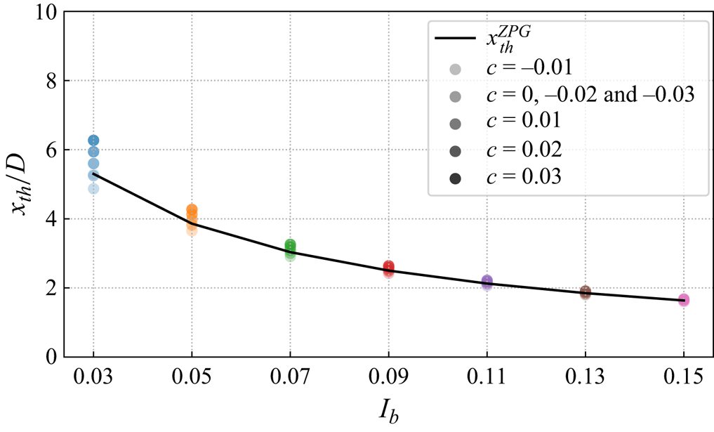
It can be seen that the near-wake length is more sensitive to the variation of  $I_b$ than
 $c$, which can be captured by (B4) very well. The influence of pressure gradient on the near-wake length significantly depends on the ambient turbulence intensity. The smaller the
 $I_b$, the more obvious influence of
 $c$. Similar to (B3), we can also define the case-averaged mean absolute percentage error for
 $x_{th}$ as follows:
 \begin{equation} \overline{{\rm MAPE}}_{x_{th}}=\frac{100\,\%}{N_{I_b}N_c}\sum_{I_b}\sum_{c} \frac{|x_{th}^{ZPG}(I_b)-x_{th}^{PG}(I_b,c)|}{x_{th}^{ZPG}(I_b)}, \end{equation}
where  $N_{I_b}=7$ and
 $N_c=7$ are the number of different
 $I_b$ and
 $c$ cases, respectively. Based on the atmospheric states considered in table 5,
 $\overline {{\rm MAPE}}_{x_{th}}=1.3\,\%$. In view of its comparable accuracy, low computational cost and robustness with respect to its counterpart under pressure gradient, we use (B4) as the near-wake length model in the study.
Appendix C. WFFAMs based on the empirical superposition principles
The proposed five empirical WFFAMs have differences in the definition of the base flow, the calculation of individual velocity deficits and the superposition principle. According to these differences, the five empirical WFFAMs can be classified into three categories.
C.1. PG-GL and PG-GS WFFAMs
These two models use the base flow  $U_b(x)$ as the background velocity to calculate individual velocity deficits, and their main difference is how to merge the individual velocity deficits. The code implementation of these two methods is very similar, so they are gathered together as follows.
(1) Calculate the single-turbine wake quantities of
$WT_i\ (1\leq i\leq N)$ under ZPG. Except for $I_u^i=I_b$, other details are the same as step (1) in Appendix A and thus not repeated here.(2) Normalised maximum velocity deficit of
$WT_i$ under pressure gradient $\rightarrow C^i(x)=C_0^i(x)[{U_b(x_i)}/{U_b(x)}]^{5/3}$.(3) Wake width of
$WT_i$ under pressure gradient $\rightarrow \sigma ^i(x)=\sigma _0^i(x)[{U_b(x_i)}/{U_b(x)}]^{2/3}$.(4) Wake velocity deficit of
$WT_i$ under pressure gradient based on $U_b(x)$ $\rightarrow u_s^i(x,y,z)=U_b(x)C^i(x)\exp (-{[(y-y_i)^2+(z-z_i)^2]}/{2(\sigma ^i)^2})$.(5) Calculate the wind-farm velocity deficit
$U_s(x,y,z)$ using the linear/square superposition principles:
(i) PG-GL:
$U_s(x,y,z)=\sum _{i=1}^{N} u_s^i(x,y,z)$;(ii) PG-GS:
$U_s(x,y,z)=\sqrt {\sum _{i=1}^{N} u_s^i(x,y,z)^2}$.


C.2. PG-LL and PG-LS WFFAMs
The main difference between these two local WFFAMs from the global WFFAMs is the calculation of base flow  $u_b^i$ for downstream turbines, which should be determined by a recursive procedure. By definition,
 $u_b^1(x)=U_b(x)$. The code implementation of these two methods is very similar, with minor differences in the superposition principle, so they are presented together as follows.
(1) Calculate the single turbine wake quantities of
$WT_i\ (1\leq i\leq N)$ under ZPG. The detail is the same as step (1) in Appendix A and thus not repeated here.(2) Assume that there are
$n$ wind turbines with the initial value $n=1$, and calculate the wind-farm velocity deficit $U_s^n$ for $n$ wind turbines.
(2.1) Normalised maximum velocity deficit of
$WT_i\ (1\leq i\leq n)$ under pressure gradient $\rightarrow C^i(x)=C_0^i(x)[{u_b^i(x_i)}/{u_b^i(x)}]^{5/3}$.(2.2) Wake width of
$WT_i\ (1\leq i\leq n)$ under pressure gradient $\rightarrow \sigma ^i(x)=\sigma _0^i(x)[{u_b^i(x_i)}/{u_b^i(x)}]^{2/3}$.(2.3) Wake velocity deficit of
$WT_i\ (1\leq i\leq n)$ under pressure gradient based on $u_b^i(x) \rightarrow u_s^i(x,y,z)=u_b^i(x)C^i(x)\exp (-{[(y-y_i)^2+(z-z_i)^2]}/{2(\sigma ^i)^2})$.(2.4) Calculate the wind-farm velocity deficit
$U_s^n(x,y,z)$ using the linear/square superposition principles:
(i) PG-LL:
$U_s^n(x,y,z)=\sum _{i=1}^{n} u_s^i(x,y,z)$;(ii) PG-LS:
$U_s^n(x,y,z)=\sqrt {\sum _{i=1}^{n} u_s^i(x,y,z)^2}$.
(3) Update the base flow
$u_b^{n+1}$ for $WT_{n+1}$ based on the definition $u_b^{n+1}(x)=U_b(x)-({1}/{N_q})\sum _{q=1}^{N_q}U_s^{n}(x,y_{n+1,q},z_{n+1,q})$.(4) Compare
$n$ and $N$. If $n=N$, output $U_s^n$; otherwise, $n=n+1$ and repeat steps (2)–(4).


C.3. PG-WP WFFAM
The essence of the wind product method is different from the above superposition methods, in which the wind-farm flow velocity deficit  $U_s$ is determined by the superposition of individual wake velocity deficits. In the wind product method,
 $U_s$ is determined by subtracting the wind-farm flow
 $U_w$ from the base flow
 $U_b(x)$, in which
 $U_w$ is calculated by a product between the base flow and the normalised individual wake velocity. Therefore, its code implementation has some differences from other empirical methods, and the details are presented in the following.
(1) Calculate the single-turbine wake quantities of
$WT_i\ (1\leq i\leq N)$ under ZPG. The detail is the same as step (1) in Appendix A and thus not repeated here.(2) Assume that there are
$n$ wind turbines with the initial value $n=1$, and calculate the wind-farm velocity deficit $U_s^n$ for $n$ wind turbines.
(2.1) Normalised maximum velocity deficit of
$WT_i\ (1\leq i\leq n)$ under pressure gradient $\rightarrow C^i(x)=C_0^i(x)[{u_b^i(x_i)}/{u_b^i(x)}]^{5/3}$.(2.2) Wake width of
$WT_i\ (1\leq i\leq n)$ under pressure gradient $\rightarrow \sigma ^i(x)=\sigma _0^i(x)[{u_b^i(x_i)}/{u_b^i(x)}]^{2/3}$.(2.3) Normalised wake velocity deficit of
$WT_i\ (1\leq i\leq n)$ under pressure gradient $\rightarrow u_s^i(x,y,z)/u_b^i(x)=C^i(x)\exp (-{[(y-y_i)^2+(z-z_i)^2]}/{2(\sigma ^i)^2})$.(2.4) Calculate the wind-farm velocity deficit
$U_s^n(x,y,z)\rightarrow U_s^n(x,y,z)=U_b(x)-U_b(x)\prod _{i=1}^{n} [1-u_s^i(x,y,z)/u_b^i(x)]$.
(3) Update the background velocity
$u_b^{n+1}$ for $WT_{n+1}$ based on the definition $u_b^{n+1}(x)=U_b(x)-({1}/{N_q})\sum _{q=1}^{N_q}U_s^{n}(x,y_{n+1,q},z_{n+1,q})$.(4) Compare
$n$ and $N$. If $n=N$, output $U_s^n$; otherwise, $n=n+1$ and repeat steps (2)–(4).