1.1 Asymptotics of the Steklov spectrum

The Steklov eigenvalues of a bounded Euclidean domain $\unicode[STIX]{x1D6FA}\subset \mathbb{R}^{d}$ are the real numbers $\unicode[STIX]{x1D70E}\in \mathbb{R}$ for which there exists a non-zero harmonic function $u:\unicode[STIX]{x1D6FA}\rightarrow \mathbb{R}$ such that $\unicode[STIX]{x2202}_{n}u=\unicode[STIX]{x1D70E}u$ on the boundary $\unicode[STIX]{x2202}\unicode[STIX]{x1D6FA}$ . Here $\unicode[STIX]{x2202}_{n}$ denotes the outward normal derivative, which exists almost everywhere provided the boundary $\unicode[STIX]{x2202}\unicode[STIX]{x1D6FA}$ is Lipschitz. Under this assumption, it is known that for $d\geqslant 2$ the Steklov spectrum is discrete (see [Reference Agranovich1]) and is given by the increasing sequence of eigenvalues $0=\unicode[STIX]{x1D70E}_{0}<\unicode[STIX]{x1D70E}_{1}\leqslant \unicode[STIX]{x1D70E}_{2}\leqslant \cdots {\nearrow}\infty ,$ where each eigenvalue is repeated according to its multiplicity. The counting function $N:\mathbb{R}\rightarrow \mathbb{N}$ is then defined by $N(\unicode[STIX]{x1D70E}):=\#\{j\in \mathbb{N}:\unicode[STIX]{x1D70E}_{j}<\unicode[STIX]{x1D70E}\}.$ For domains with smooth boundary, one can show using pseudodifferential techniques that the counting function satisfies Weyl’s law

(1.1.1) $$\begin{eqnarray}\displaystyle N(\unicode[STIX]{x1D70E})=\frac{\unicode[STIX]{x1D714}_{d-1}}{(2\unicode[STIX]{x1D70B})^{d-1}}\text{Vol}_{d-1}(\unicode[STIX]{x2202}\unicode[STIX]{x1D6FA})\unicode[STIX]{x1D70E}^{d-1}+O(\unicode[STIX]{x1D70E}^{d-2})\quad \text{as }\unicode[STIX]{x1D70E}{\nearrow}+\infty , & & \displaystyle\end{eqnarray}$$

where $\unicode[STIX]{x1D714}_{d-1}$ is the measure of the unit ball $B_{1}(0)\subset \mathbb{R}^{d-1}.$ The remainder estimate in (1.1.1) is sharp and attained on a round ball. Moreover, a two-term asymptotic formula for the counting function holds under a non-periodicity condition of the geodesic flow on $\unicode[STIX]{x2202}\unicode[STIX]{x1D6FA}$ (see [Reference Polterovich and Sher14, formula (5.1.8)]).

Understanding precise asymptotics for Steklov eigenvalues on domains with singularities, such as corners and edges, is significantly more challenging, since pseudodifferential techniques do not work in this case (see [Reference Girouard and Polterovich5, §3] for a discussion). Using variational methods, one can prove a one-term Weyl asymptotic formula that holds for any piecewise $C^{1}$ Euclidean domain (see [Reference Agranovich1]):

(1.1.2) $$\begin{eqnarray}\displaystyle N(\unicode[STIX]{x1D70E})=\frac{\unicode[STIX]{x1D714}_{d-1}}{(2\unicode[STIX]{x1D70B})^{d-1}}\text{Vol}_{d-1}(\unicode[STIX]{x2202}\unicode[STIX]{x1D6FA})\unicode[STIX]{x1D70E}^{d-1}+o(\unicode[STIX]{x1D70E}^{d-1})\quad \text{as }\unicode[STIX]{x1D70E}{\nearrow}+\infty . & & \displaystyle\end{eqnarray}$$

However, in order to get sharper asymptotics, one needs to understand the contribution of singularities to the counting function. In two dimensions, some results in this direction have been recently obtained in [Reference Levitin, Parnovski, Polterovich and Sher12]. In the present paper we aim to explore the most basic higher-dimensional example: the Euclidean cuboids.

1.2 Main result

Given $d\in \mathbb{N}$ , the cuboid Footnote ¹ with parameters $a_{1},\ldots ,a_{d}>0$ is defined as a product of the intervals

$$\begin{eqnarray}\unicode[STIX]{x1D6FA}=(-a_{1},a_{1})\times (-a_{2},a_{2})\times \cdots \times (-a_{d},a_{d})\subset \mathbb{R}^{d}.\end{eqnarray}$$

If $a_{1}=a_{2}=\cdots =a_{d}$ we say that $\unicode[STIX]{x1D6FA}$ is a cube. The main result of this paper is the following theorem.

Theorem 1.1. Let $\unicode[STIX]{x1D6FA}\subset \mathbb{R}^{d}$ be the cuboid with parameters $a_{1},\ldots ,a_{d}>0$ . For $d\geqslant 3$ , the counting function of Steklov eigenvalues satisfies a two-term asymptotic formula as $\unicode[STIX]{x1D70E}\rightarrow \infty$ :

(1.2.1) $$\begin{eqnarray}\displaystyle N(\unicode[STIX]{x1D70E})=C_{1}\text{Vol}_{d-1}(\unicode[STIX]{x2202}\unicode[STIX]{x1D6FA})\unicode[STIX]{x1D70E}^{d-1}+C_{2}\text{Vol}_{d-2}(\unicode[STIX]{x2202}^{2}\unicode[STIX]{x1D6FA})\unicode[STIX]{x1D70E}^{d-2}+O(\unicode[STIX]{x1D70E}^{\unicode[STIX]{x1D702}}),\qquad & & \displaystyle\end{eqnarray}$$

where $\unicode[STIX]{x2202}^{2}\unicode[STIX]{x1D6FA}$ denotes the union of all the $(d-2)$ -dimensional facets of $\unicode[STIX]{x1D6FA}$ . Here $\unicode[STIX]{x1D702}=2/3$ for $d=3$ and $\unicode[STIX]{x1D702}=d-2-1/(d-1)$ for $d\geqslant 4$ . The constants $C_{1}$ and $C_{2}$ are given by

$$\begin{eqnarray}\displaystyle C_{1}=\frac{\unicode[STIX]{x1D714}_{d-1}}{(2\unicode[STIX]{x1D70B})^{d-1}} & & \displaystyle \nonumber\end{eqnarray}$$

and

$$\begin{eqnarray}\displaystyle C_{2}=\frac{2^{(d-2)/2}\unicode[STIX]{x1D714}_{d-2}}{(2\unicode[STIX]{x1D70B})^{d-2}}-\frac{2G_{d-1,1}}{\unicode[STIX]{x1D70B}^{d-1}}-\frac{\unicode[STIX]{x1D714}_{d-2}}{2(2\unicode[STIX]{x1D70B})^{d-2}}, & & \displaystyle \nonumber\end{eqnarray}$$

where

$$\begin{eqnarray}\displaystyle G_{d-1,1}=\underbrace{\int _{0}^{\unicode[STIX]{x1D70B}/2}\cdots \int _{0}^{\unicode[STIX]{x1D70B}/2}}_{d-2}\text{arccot}\biggl(\mathop{\prod }_{j=1}^{d-2}\csc \unicode[STIX]{x1D703}_{j}\biggr)\mathop{\prod }_{k=1}^{d-2}\sin ^{k}(\unicode[STIX]{x1D703}_{k})\,d\unicode[STIX]{x1D703}_{1}\ldots \,d\unicode[STIX]{x1D703}_{d-2}. & & \displaystyle \nonumber\end{eqnarray}$$

For $d=2$ , the counting function admits a one-term asymptotics

$$\begin{eqnarray}\displaystyle N(\unicode[STIX]{x1D70E})=\unicode[STIX]{x1D70B}^{-1}\text{Vol}_{1}(\unicode[STIX]{x2202}\unicode[STIX]{x1D6FA})\unicode[STIX]{x1D70E}+O(1). & & \displaystyle \nonumber\end{eqnarray}$$

Remark 1.2. It can be shown that $C_{2}>0$ for all $d\geqslant 3$ , see Appendix B. The constants $G_{d,1}$ are special cases of constants $G_{p,q}$ which will be introduced in §3. The constants $G_{2,1}$ and $G_{3,1}$ can be computed explicitly as

$$\begin{eqnarray}\displaystyle G_{2,1} & = & \displaystyle {\textstyle \frac{1}{2}}(-1+\sqrt{2})\unicode[STIX]{x1D70B},\nonumber\\ \displaystyle G_{3,1} & = & \displaystyle {\textstyle \frac{1}{8}}(-2+\unicode[STIX]{x1D70B})\unicode[STIX]{x1D70B}.\nonumber\end{eqnarray}$$

Remark 1.4. For $d=3$ , Theorem 1.1 implies that

$$\begin{eqnarray}{\mathcal{R}}(\unicode[STIX]{x1D70E})=\frac{N(\unicode[STIX]{x1D70E})-C_{1}\text{Vol}_{2}(\unicode[STIX]{x2202}\unicode[STIX]{x1D6FA})\unicode[STIX]{x1D70E}^{2}-C_{2}\text{Vol}_{1}(\unicode[STIX]{x2202}^{2}\unicode[STIX]{x1D6FA})\unicode[STIX]{x1D70E}}{\unicode[STIX]{x1D70E}^{2/3}}\end{eqnarray}$$

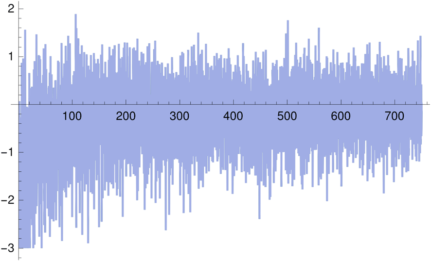
is a bounded function of $\unicode[STIX]{x1D70E}$ . In order to validate the expression for the constant $C_{2}$ obtained in Theorem 1.1, we have checked numerically that this claim holds, using the approximate eigenvalues introduced in §3 on a cube with side lengths $2$ . Figure 1 shows that $|{\mathcal{R}}(\unicode[STIX]{x1D70E})|\leqslant 3$ for $\unicode[STIX]{x1D70E}<750$ which corresponds to approximately a million eigenvalues.

Figure 1

$(N(\unicode[STIX]{x1D70E})-C_{1}\text{Vol}_{2}(\unicode[STIX]{x2202}\unicode[STIX]{x1D6FA})\unicode[STIX]{x1D70E}^{2}-C_{2}\text{Vol}_{1}(\unicode[STIX]{x2202}^{2}\unicode[STIX]{x1D6FA})\unicode[STIX]{x1D70E})/\unicode[STIX]{x1D70E}^{2/3}$ for $\unicode[STIX]{x1D70E}<750$ .

1.3 Outline of the proof

The proof of Theorem 1.1 is given in §3. The outline of the argument is as follows. First, we show that the Steklov eigenvalue problem on a cuboid admits separation of variables, see Lemma 2.1 below. Separation of variables yields eigenfunctions that are products of trigonometric, hyperbolic and possibly linear factors. One can check that the number of eigenvalues corresponding to eigenfunctions containing linear terms is at most finite, see Theorem 2.6. The same theorem also shows that the eigenvalue counting problem can be reduced to a family of approximate lattice counting problems. More specifically, given $1\leqslant p\leqslant d$ , we consider the counting function $N_{p}$ of eigenvalues corresponding to eigenfunctions with exactly $p$ trigonometric factors. It turns out that for each $p>1$ , the counting function $N_{p}$ satisfies a two-term asymptotic formula, see Proposition 3.1. The functions $N_{p}$ for $p=d-1$ and $p=d-2$ are the dominant ones. In particular, the main term in (1.2.1) corresponds to the main term in the asymptotics for $N_{d-1}$ . The second term in (1.2.1) is obtained as a sum of the main term in the asymptotics of $N_{d-2}$ and the second term in $N_{d-1}$ . The latter also splits into two parts: one is the standard contribution of overcounted lattice points (see Lemma 3.17), and the other has to do with the geometry of the domain $E_{\unicode[STIX]{x1D70E}}$ defined by (3.4.12) arising in the lattice counting problem. While this domain $E_{\unicode[STIX]{x1D70E}}$ converges to a ball as $\unicode[STIX]{x1D70E}\rightarrow \infty$ , the approximation produces an error that contributes to the second term of (1.2.1). This explains why the coefficient $C_{2}$ is represented by a sum of three constants. Note that while two of these constants are negative, the coefficient $C_{2}$ is always positive; see Appendix B.

1.5 An isoperimetric inequality for the first Steklov eigenvalue

Given a cuboid $\unicode[STIX]{x1D6FA}\subset \mathbb{R}^{d}$ with parameters $a_{1},\ldots ,a_{d}>0$ , let $\unicode[STIX]{x1D6FA}^{\star }$ and $\unicode[STIX]{x1D6FA}^{\sharp }$ be the cubes such that

$$\begin{eqnarray}\text{Vol}_{d-1}\unicode[STIX]{x2202}\unicode[STIX]{x1D6FA}^{\star }=\text{Vol}_{d-1}\unicode[STIX]{x2202}\unicode[STIX]{x1D6FA}\quad \text{and}\quad \text{Vol}_{d}\unicode[STIX]{x1D6FA}^{\sharp }=\text{Vol}_{d}\unicode[STIX]{x1D6FA}.\end{eqnarray}$$

The proof of the theorem is presented in §4.3. In a way, it is not surprising that the cube, being the most symmetric of all cuboids, maximizes $\unicode[STIX]{x1D70E}_{1}$ under both volume and surface area restrictions. Theorem 1.6 could be compared with the well-known Weinstock’s inequality [Reference Weinstock19] stating that the disk is a unique maximizer for $\unicode[STIX]{x1D70E}_{1}$ among planar simply connected domains with a given perimeter (see also a recent generalization of this result for convex domains in higher dimensions obtained in [Reference Bucur, Ferone, Nitsch and Trombetti4]), as well as with Brock’s result [Reference Brock3] which states that balls are unique maximizers among Euclidean domains $\unicode[STIX]{x1D6FA}\subset \mathbb{R}^{d}$ with prescribed $d$ –volume.

It follows from Theorem 1.6 that any cube is spectrally determined among all cuboids.

Note that a similar corollary with an almost identical proof holds for planar simply-connected domains, among which the disk is spectrally determined, using the case of equality in Weinstock’s theorem [Reference Weinstock19].

It is still unknown whether there exist non-isometric Steklov isospectral Euclidean domains. Our results imply that if two rectangles are Steklov isospectral, they are isometric.

The proof of this corollary is presented in §4.4. Let us conclude the introduction with the following conjecture.

Plan of the paper. In §2, we explore the structure of Steklov eigenvalues and eigenfunctions on cuboids. In particular, in §2.1 we describe separation of variables and prove that it yields a complete system of Steklov eigenfunctions. In §2.2 a classification of eigenfunctions is presented based on the number of linear, trigonometric and hyperbolic terms, which is later used in §2.3 to reduce the problem of counting eigenvalues to counting approximate lattice points. Theorem 1.1 is proved in §3. This is the most technically involved part of the paper, involving tools from analytic number theory and Fourier analysis. Other results of the paper are proved in §4. In particular, a somewhat surprising observation that Steklov eigenfunctions may concentrate on lower-dimensional facets of cuboids is presented in §4.1. Sections 4.3 and 4.4 provide the proofs of Theorem 1.6 and Corollary 1.8. Appendix A contains the proof of an auxiliary Lemma A.1 used in §3.4. In Appendix B we justify the positivity of the constant $C_{2}$ as stated in Remark 1.2.

2.1 Separation of variables

The following lemma shows that the method of separation of variables is applicable to the computation of the Steklov spectrum of a product of compact manifolds with boundary. In particular, we justify completeness of the system of Steklov eigenfunctions admitting separation of variables.

Lemma 2.1. Let $M_{1}$ and $M_{2}$ be smooth compact Riemannian manifolds with boundary. Let $\unicode[STIX]{x1D70E}\geqslant 0$ be a Steklov eigenvalue of the product manifold $M=M_{1}\times M_{2}$ with the eigenspace $F_{\unicode[STIX]{x1D70E}}\subset L^{2}(M)$ . There exists a basis $(u^{(1)},\ldots ,u^{(m)})$ of $F_{\unicode[STIX]{x1D70E}}$ such that each $u^{(j)}:M_{1}\times M_{2}\rightarrow \mathbb{R}$ is separable:

$$\begin{eqnarray}\displaystyle u^{(j)}(x_{1},x_{2})=u_{1}^{(j)}(x_{1})u_{2}^{(j)}(x_{2}),\quad 1\leqslant j\leqslant m, & & \displaystyle \nonumber\end{eqnarray}$$

where $u_{1}^{(j)}:M_{1}\rightarrow \mathbb{R}$ and $u_{2}^{(j)}:M_{2}\rightarrow \mathbb{R}$ .

Proof. Consider the Robin problem with parameter $\unicode[STIX]{x1D70E}\geqslant 0$ on $M$

$$\begin{eqnarray}\displaystyle \left\{\begin{array}{@{}ll@{}}\unicode[STIX]{x1D6E5}u+\unicode[STIX]{x1D706}u=0\quad & \text{in }M,\\ \unicode[STIX]{x2202}_{n}u=\unicode[STIX]{x1D70E}u\quad & \text{on }\unicode[STIX]{x2202}M.\end{array}\right. & & \displaystyle \nonumber\end{eqnarray}$$

It is well known that the Robin problem on $M$ admits separation of variables, since $L^{2}(M)=L^{2}(M_{1})\otimes L^{2}(M_{2})$ is a product space, see e.g., [Reference Strauss16, §11.5]. The number $\unicode[STIX]{x1D70E}\geqslant 0$ is a Steklov eigenvalue of $M$ if and only if $0$ is an eigenvalue of the Robin problem with parameter $\unicode[STIX]{x1D70E}$ , and the corresponding eigenspace is the same for both problems. Since one can find a separated eigenbasis for $F_{\unicode[STIX]{x1D70E}}$ by virtue of it being a Robin eigenspace on $M$ , it then suffices to use the same basis for $F_{\unicode[STIX]{x1D70E}}$ when we consider it as a Steklov eigenspace.◻

Let $d\in \mathbb{N}$ and consider the cuboid $\unicode[STIX]{x1D6FA}$ with parameters $a_{1},\ldots ,a_{d}>0$ . Because $\unicode[STIX]{x1D6FA}$ is a product of compact intervals, it follows from Lemma 2.1 that there exists a complete set $\{{u_{j}\}}_{j\in \mathbb{N}_{0}}$ of separated Steklov eigenfunctions on $\unicode[STIX]{x1D6FA}$ . Consider a function $u:\unicode[STIX]{x1D6FA}\rightarrow \mathbb{R}$ given by the product $u(x)=u_{1}(x_{1})\cdots u_{d}(x_{d})$ , where $u_{j}:[-a_{j},a_{j}]\rightarrow \mathbb{R}$ . Requiring $u$ to be a Steklov eigenfunction with eigenvalue $\unicode[STIX]{x1D70E}\geqslant 0$ leads to numbers $\unicode[STIX]{x1D706}_{1},\unicode[STIX]{x1D706}_{2},\ldots ,\unicode[STIX]{x1D706}_{d}\in \mathbb{R}$ such that

(2.1.1) $$\begin{eqnarray}\displaystyle \left\{\begin{array}{@{}l@{}}u_{j}^{\prime \prime }+\unicode[STIX]{x1D706}_{j}u_{j}=0\quad \text{on }(-a_{j},a_{j}),\quad \\ u_{j}^{\prime }(a_{j})=\unicode[STIX]{x1D70E}u_{j}(a_{j}),\quad \\ -u_{j}^{\prime }(-a_{j})=\unicode[STIX]{x1D70E}u_{j}(-a_{j}),\quad \end{array}\right. & & \displaystyle\end{eqnarray}$$

subject to the harmonicity condition

(2.1.2) $$\begin{eqnarray}\displaystyle \mathop{\sum }_{j=1}^{d}\unicode[STIX]{x1D706}_{j}=0. & & \displaystyle\end{eqnarray}$$

The following lemma describes the eigenvalues and eigenfunctions of the auxiliary one-dimensional Steklov spectral problem (2.1.1) with a parameter $\unicode[STIX]{x1D706}\in \mathbb{R}$ .

Lemma 2.4. Let $\unicode[STIX]{x1D706}\in \mathbb{R}$ . The non-zero solutions $\unicode[STIX]{x1D711}:[-a,a]\rightarrow \mathbb{R}$ of the differential equation $\unicode[STIX]{x1D711}^{\prime \prime }+\unicode[STIX]{x1D706}\unicode[STIX]{x1D711}=0$ subject to the boundary conditions

$$\begin{eqnarray}\displaystyle \unicode[STIX]{x1D711}^{\prime }(a)=\unicode[STIX]{x1D70E}\unicode[STIX]{x1D711}(a)\quad \text{and}\quad -\unicode[STIX]{x1D711}^{\prime }(-a)=\unicode[STIX]{x1D70E}\unicode[STIX]{x1D711}(-a) & & \displaystyle \nonumber\end{eqnarray}$$

for some constant $\unicode[STIX]{x1D70E}\geqslant 0$ are constant multiples of one the following functions:

1. (i) for $\unicode[STIX]{x1D706}=0$ , $\unicode[STIX]{x1D711}(t)\equiv 1$ and $\unicode[STIX]{x1D70E}=0$ or $\unicode[STIX]{x1D711}(t)=t\text{ and }\unicode[STIX]{x1D70E}=a^{-1}$ ;

2. (ii) for $\unicode[STIX]{x1D706}=\unicode[STIX]{x1D6FC}^{2}>0$ , one of

   $$\begin{eqnarray}\displaystyle \unicode[STIX]{x1D711}(t) & = & \displaystyle \sin (\unicode[STIX]{x1D6FC}t)\quad \text{with }\unicode[STIX]{x1D70E}=\unicode[STIX]{x1D6FC}\cot (\unicode[STIX]{x1D6FC}a),\nonumber\\ \displaystyle \unicode[STIX]{x1D711}(t) & = & \displaystyle \cos (\unicode[STIX]{x1D6FC}t)\quad \text{with }\unicode[STIX]{x1D70E}=-\unicode[STIX]{x1D6FC}\tan (\unicode[STIX]{x1D6FC}a)\nonumber\end{eqnarray}$$
   (in other words, for each $\ell \in \{0,1\}$ , $\unicode[STIX]{x1D70E}=\unicode[STIX]{x1D6FC}\cot (\unicode[STIX]{x1D6FC}a+\ell (\unicode[STIX]{x1D70B}/2))$ is an eigenvalue);

3. (iii) for $\unicode[STIX]{x1D706}=-\unicode[STIX]{x1D6FD}^{2}<0$ , one of

   $$\begin{eqnarray}\displaystyle \unicode[STIX]{x1D711}(t) & = & \displaystyle \sinh (\unicode[STIX]{x1D6FD}t)\quad \text{with }\unicode[STIX]{x1D70E}=\unicode[STIX]{x1D6FD}\coth (\unicode[STIX]{x1D6FD}a),\nonumber\\ \displaystyle \unicode[STIX]{x1D711}(t) & = & \displaystyle \cosh (\unicode[STIX]{x1D6FD}t)\quad \text{with }\unicode[STIX]{x1D70E}=\unicode[STIX]{x1D6FD}\tanh (\unicode[STIX]{x1D6FD}a)\nonumber\end{eqnarray}$$
   (in other words, for each $j\in \{-1,1\}$ , $\unicode[STIX]{x1D70E}=\unicode[STIX]{x1D6FD}\tanh (\unicode[STIX]{x1D6FD}a)^{j}$ is an eigenvalue).

It will be useful to introduce a uniform notation for these eigenvalues. Given $a>0$ and $\ell \in \{0,1\}$ , let

$$\begin{eqnarray}\displaystyle T_{a,\ell }(x)=x\cot \biggl(ax+\ell \frac{\unicode[STIX]{x1D70B}}{2}\biggr)=\left\{\begin{array}{@{}ll@{}}x\cot (ax)\quad & \text{for }\ell =0,\\ -x\tan (ax)\quad & \text{for }\ell =1,\end{array}\right. & & \displaystyle \nonumber\end{eqnarray}$$

and

$$\begin{eqnarray}\displaystyle H_{a,\ell }(x)=\left\{\begin{array}{@{}ll@{}}x\coth (ax)\quad & \text{for }\ell =0,\\ x\tanh (ax)\quad & \text{for }\ell =1.\end{array}\right. & & \displaystyle \nonumber\end{eqnarray}$$

It follows from Lemma 2.4 that separable eigenfunctions are products of linear factors, trigonometric factors (the function $\sin$ for $\ell =0$ , and $\cos$ for $\ell =1$ ) and hyperbolic factors (the function $\sinh$ for $\ell =0$ , and $\cosh$ for $\ell =1$ ). A careful accounting of these will be presented.

2.2 Classification of eigenfunctions

It follows from the previous paragraph that there is a complete set of Steklov eigenfunctions given by products of linear, trigonometric and hyperbolic factors. They are of the form

(2.2.1) $$\begin{eqnarray}\displaystyle u(x_{1},\ldots ,x_{d})=\mathop{\prod }_{i\in \unicode[STIX]{x1D70F}_{0}}x_{i}\mathop{\prod }_{j\in \unicode[STIX]{x1D70F}_{1}}\text{Trig}_{j}(\unicode[STIX]{x1D6FC}_{j}x_{\!j})\mathop{\prod }_{k\in \unicode[STIX]{x1D70F}_{2}}\text{Hyp}_{k}(\unicode[STIX]{x1D6FD}_{k}x_{k}), & & \displaystyle\end{eqnarray}$$

where $\unicode[STIX]{x1D70F}_{0},\unicode[STIX]{x1D70F}_{1},\unicode[STIX]{x1D70F}_{2}$ are disjoint subsets of $S_{d}:=\{1,2,\ldots ,d\}$ such that $\unicode[STIX]{x1D70F}_{0}\cup \unicode[STIX]{x1D70F}_{1}\cup \unicode[STIX]{x1D70F}_{2}=S_{d}$ , and each $\text{Trig}_{j}\in \{\sin ,\cos \}$ and $\text{Hyp}_{k}\in \{\sinh ,\cosh \}$ . In order for this function to be a Steklov eigenfunction corresponding to the eigenvalue $\unicode[STIX]{x1D70E}>0$ , the function $u$ must be harmonic. This amounts to the following restatement of condition (2.1.2) in terms of the constants $\unicode[STIX]{x1D6FC}_{j}$ and $\unicode[STIX]{x1D6FD}_{k}$ :

(2.2.2) $$\begin{eqnarray}\displaystyle \mathop{\sum }_{j\in \unicode[STIX]{x1D70F}_{1}}\unicode[STIX]{x1D6FC}_{j}^{2}=\mathop{\sum }_{k\in \unicode[STIX]{x1D70F}_{2}}\unicode[STIX]{x1D6FD}_{k}^{2}. & & \displaystyle\end{eqnarray}$$

This equation will be called the harmonicity condition. Moreover, the spectral parameter $\unicode[STIX]{x1D70E}$ has to be the same on each face of the cuboid. By Lemma 2.4 this translates into the following equations, called the compatibility conditions:

(2.2.3) $$\begin{eqnarray}\displaystyle \unicode[STIX]{x1D70E}=\left\{\begin{array}{@{}ll@{}}a_{i}^{-1}\quad & \text{for }i\in \unicode[STIX]{x1D70F}_{0},\\ T_{a_{i},\ell (i)}(\unicode[STIX]{x1D6FC}_{i})\quad & \text{for }i\in \unicode[STIX]{x1D70F}_{1},\\ H_{a_{i},\ell (i)}(\unicode[STIX]{x1D6FD}_{i})\quad & \text{for }i\in \unicode[STIX]{x1D70F}_{2}.\end{array}\right. & & \displaystyle\end{eqnarray}$$

Here the function $\ell :S_{d}\rightarrow \{0,1\}$ is used to specify which trigonometric and hyperbolic functions are used, according to the convention introduced in Lemma 2.4. The corresponding eigenfunction (2.2.1) is then given precisely by the product of the factors $u_{i}:[-a_{i},a_{i}]\rightarrow \mathbb{R}$ which are specified by

(2.2.4) $$\begin{eqnarray}\displaystyle u_{i}(x_{i})=\left\{\begin{array}{@{}ll@{}}\text{Trig}_{\ell (i)}(\unicode[STIX]{x1D6FC}_{i}x_{i})\quad & \text{for }i\in \unicode[STIX]{x1D70F}_{1},\\ \text{Hyp}_{\ell (i)}(\unicode[STIX]{x1D6FD}_{i}x_{i})\quad & \text{for }i\in \unicode[STIX]{x1D70F}_{2},\\ x_{i}\quad & \text{otherwise},\end{array}\right. & & \displaystyle\end{eqnarray}$$

where $\text{Trig}_{0}=\sin$ , $\text{Trig}_{1}=\cos$ , $\text{Hyp}_{0}=\sinh$ and $\text{Hyp}_{1}=\cosh$ .

Note that any separated eigenfunction that has a linear factor $u_{j}(x_{\!j})=x_{\!j}$ contributes the eigenvalue $\unicode[STIX]{x1D70E}=a_{j}^{-1}$ to the spectrum. Since the multiplicity of each eigenvalue is finite, this can occur at most a finite number of times. We summarize the above mentioned facts in the following theorem.

Theorem 2.5. Let $p\in \{1,\ldots ,d-1\}$ , and let ${\mathcal{T}}_{p}$ be the set of all ordered bipartitions $\unicode[STIX]{x1D70F}=(\unicode[STIX]{x1D70F}_{1},\unicode[STIX]{x1D70F}_{2})$ of $\{1,\ldots ,d\}$ in the sets of cardinality $p$ and $q=d-p$ . For each $\unicode[STIX]{x1D70F}\in {\mathcal{T}}_{p}$ and any $\ell :\unicode[STIX]{x1D70F}_{1}\cup \unicode[STIX]{x1D70F}_{2}\rightarrow \{0,1\}$ , let $S_{\unicode[STIX]{x1D70F},\ell }$ be the set of all numbers $\unicode[STIX]{x1D70E}>0$ for which there exist positive numbers $\unicode[STIX]{x1D6FC}_{i}$ for $i\in \unicode[STIX]{x1D70F}_{1}$ and $\unicode[STIX]{x1D6FD}_{j}$ , for $j\in \unicode[STIX]{x1D70F}_{2}$ , which solve

$$\begin{eqnarray}\displaystyle \unicode[STIX]{x1D70E}=T_{a_{i},\ell (i)}(\unicode[STIX]{x1D6FC}_{i})=H_{a_{j},\ell (j)}(\unicode[STIX]{x1D6FD}_{j})\quad \text{for all }i\in \unicode[STIX]{x1D70F}_{1},j\in \unicode[STIX]{x1D70F}_{2} & & \displaystyle \nonumber\end{eqnarray}$$

subject to the constraint

$$\begin{eqnarray}\displaystyle \mathop{\sum }_{i\in \unicode[STIX]{x1D70F}_{1}}\unicode[STIX]{x1D6FC}_{i}^{2}=\mathop{\sum }_{j\in \unicode[STIX]{x1D70F}_{2}}\unicode[STIX]{x1D6FD}_{j}^{2}. & & \displaystyle \nonumber\end{eqnarray}$$

Denote also by $S_{0}$ the collection of Steklov eigenvalues corresponding to separated eigenfunctions having a linear factor. Then the Steklov spectrum of a cuboid $\unicode[STIX]{x1D6FA}$ is given by the union of $S_{0}$ which contains at most finitely many elements, and the families $S_{\unicode[STIX]{x1D70F},l}$ for all possible choices of $\unicode[STIX]{x1D70F}$ and $\ell$ .

2.3 Reduction to approximate lattice counting

We will now give a more precise description of the spectrum by constructing a correspondence between the Steklov eigenvalues of cuboids and the vertices of certain lattices.

Let $\unicode[STIX]{x1D6FA}$ be a cuboid with parameters $a_{1},\ldots ,a_{d}$ . Let $p\in \{1,\ldots ,d-1\}$ represent the number of trigonometric factors of a separated eigenfunction without linear factors. Each bipartition $\unicode[STIX]{x1D70F}=(\unicode[STIX]{x1D70F}_{1},\unicode[STIX]{x1D70F}_{2})\in {\mathcal{T}}_{p}$ then corresponds to a separated eigenfunction of the form

(2.3.1) $$\begin{eqnarray}\displaystyle u(x_{1},\ldots ,x_{d})=\mathop{\prod }_{j\in \unicode[STIX]{x1D70F}_{1}}\text{Trig}_{j}(\unicode[STIX]{x1D6FC}_{j}x_{\!j})\mathop{\prod }_{k\in \unicode[STIX]{x1D70F}_{2}}\text{Hyp}_{k}(\unicode[STIX]{x1D6FD}_{k}x_{k}). & & \displaystyle\end{eqnarray}$$

Let $\mathbb{N}_{0}=\{0,1,2,\ldots \}$ be the set of non-negative integers. Given $\mathbf{n}\in \mathbb{N}_{0}^{p}$ , let

$$\begin{eqnarray}I_{\mathbf{n}}=I_{\mathbf{n},p,\unicode[STIX]{x1D70F}}:=\mathop{\prod }_{i\in \unicode[STIX]{x1D70F}_{1}}\biggl(\frac{n_{i}\unicode[STIX]{x1D70B}}{2a_{i}},\frac{(n_{i}+1)\unicode[STIX]{x1D70B}}{2a_{i}}\biggr]\subset \mathbb{R}^{p}.\end{eqnarray}$$

The boxes $I_{\mathbf{n}}$ are fundamental domains of a lattice. The following theorem shows that each box gives rise to a cluster of at most $2^{q}$ eigenvalues and, moreover, the boxes $I_{\mathbf{n}}$ with $\mathbf{n}\in \mathbb{N}^{p}$ and $|\mathbf{n}|$ large enough correspond to precisely $2^{q}$ eigenvalues.

Assertions (ii) and (iii) essentially say that up to a finite number of boxes, there is always exactly $2^{q}$ solutions in the box $I_{\mathbf{n}}$ , while assertion (iv) says that while some boxes touching the coordinate hyperplanes $\{x_{\!j}=0\}$ might contain solutions, this will only happen a finite number of times. This means that while all the three cases are needed to fully describe the spectrum, asymptotically we can only count eigenvalues described by (iii), up to a $O(1)$ error.

Construction of an eigenfunction. For each $i\in \unicode[STIX]{x1D70F}_{2}$ , the function $\unicode[STIX]{x1D6FD}_{i}\mapsto H_{a_{i},\ell (i)}(\unicode[STIX]{x1D6FD}_{i})$ , is increasing and positive for $\unicode[STIX]{x1D6FD}_{i}>0$ . It satisfies $H_{a_{i},\ell (i)}(\unicode[STIX]{x1D6FD}_{i})=\unicode[STIX]{x1D6FD}_{i}+O(\unicode[STIX]{x1D6FD}_{i}^{-\infty })$ as $\unicode[STIX]{x1D6FD}_{i}\rightarrow \infty$ and

$$\begin{eqnarray}\lim _{\unicode[STIX]{x1D6FD}_{i}\rightarrow 0}H_{a_{i},\ell (i)}(\unicode[STIX]{x1D6FD}_{i})=\left\{\begin{array}{@{}ll@{}}\displaystyle \frac{1}{a_{i}}\quad & \text{if }\ell (i)=0,\\ 0\quad & \text{if }\ell (i)=1.\end{array}\right.\end{eqnarray}$$

This implies that the equations

(2.3.3) $$\begin{eqnarray}\displaystyle H_{a_{i},\ell (i)}(\unicode[STIX]{x1D6FD}_{i})=H_{a_{j},\ell (j)}(\unicode[STIX]{x1D6FD}_{j})\quad \text{for all }i,j\in \unicode[STIX]{x1D70F}_{2} & & \displaystyle\end{eqnarray}$$

define a connected curve $C_{H}=C_{H,p,\unicode[STIX]{x1D70F}}\subset \mathbb{R}^{q}$ (the index $H$ stands for “hyperbolic”) which behaves like the diagonal

$$\begin{eqnarray}\{\boldsymbol{\unicode[STIX]{x1D6FD}}\in \mathbb{R}^{q}:\unicode[STIX]{x1D6FD}_{i}=\unicode[STIX]{x1D6FD}_{j}\text{ for each }i,j\in \unicode[STIX]{x1D70F}_{2}\}\end{eqnarray}$$

to infinite order as $|\boldsymbol{\unicode[STIX]{x1D6FD}}|\rightarrow \infty$ . The common value given by equation (2.3.3) increases monotonically from some $c\geqslant 0$ to infinity along the curve $C_{H}$ as it moves away from the origin. In fact, this non-negative constant is

$$\begin{eqnarray}c_{\ell }=\max \{0,a_{i}^{-1}:i\in \unicode[STIX]{x1D70F}_{2},\ell (i)=0\}.\end{eqnarray}$$

On the other hand, for each $i\in \unicode[STIX]{x1D70F}_{1}$ the restricted function

(2.3.4) $$\begin{eqnarray}\displaystyle T_{a_{i},\ell (i)}:\biggl(\frac{n_{i}\unicode[STIX]{x1D70B}}{a_{i}}+\frac{\ell (i)\unicode[STIX]{x1D70B}}{2a_{i}},\frac{n_{i}\unicode[STIX]{x1D70B}}{a_{1}}+\frac{(\ell (i)+1)\unicode[STIX]{x1D70B}}{2a_{i}}\biggr]\longrightarrow [0,\infty ) & & \displaystyle\end{eqnarray}$$

is decreasing and surjective. Hence, for each point $\boldsymbol{\unicode[STIX]{x1D6FD}}\in C_{H}\subset \mathbb{R}^{q}$ , there exist unique numbers

$$\begin{eqnarray}\unicode[STIX]{x1D6FC}_{i}(\boldsymbol{\unicode[STIX]{x1D6FD}})\in \biggl(\frac{n_{i}\unicode[STIX]{x1D70B}}{a_{i}}+\frac{\ell (i)\unicode[STIX]{x1D70B}}{2a_{i}},\frac{n_{i}\unicode[STIX]{x1D70B}}{a_{1}}+\frac{(\ell (i)+1)\unicode[STIX]{x1D70B}}{2a_{i}}\biggr]\quad (\text{for each }i\in \unicode[STIX]{x1D70F}_{1})\end{eqnarray}$$

such that

(2.3.5) $$\begin{eqnarray}\displaystyle T_{a_{i},\ell (i)}(\unicode[STIX]{x1D6FC}_{i})=H_{a_{j},\ell (j)}(\unicode[STIX]{x1D6FD}_{j})\quad \text{for all }i\in \unicode[STIX]{x1D70F}_{1},j\in \unicode[STIX]{x1D70F}_{2}. & & \displaystyle\end{eqnarray}$$

This defines an image curve $C_{T}\subset \mathbb{R}^{p}$ given by

$$\begin{eqnarray}C_{T}=\{\unicode[STIX]{x1D6FC}_{i}(\boldsymbol{\unicode[STIX]{x1D6FD}}):i\in \unicode[STIX]{x1D70F}_{1},\boldsymbol{\unicode[STIX]{x1D6FD}}\in C_{H}\}.\end{eqnarray}$$

In other words, we have defined a continuous map $\boldsymbol{\unicode[STIX]{x1D6FC}}:C_{H}\longrightarrow C_{T}$ between these two curves. It follows from (2.3.4) that the curve $C_{T}$ is contained in the box $I_{2\mathbf{n}+\mathbf{m}}$ , where $\mathbf{m}\in \{0,1\}^{p}$ is determined by the restriction of $\ell$ to $\unicode[STIX]{x1D70F}_{1}$ . In particular, as the value of $|\boldsymbol{\unicode[STIX]{x1D6FD}}|$ increases from its minimal value to $+\infty$ along the curve $C_{H}$ , the value of $|\boldsymbol{\unicode[STIX]{x1D6FC}}(\boldsymbol{\unicode[STIX]{x1D6FD}})|$ is contained in the compact interval

$$\begin{eqnarray}\biggl[\inf _{\mathbf{x}\in I_{2\mathbf{n}+\mathbf{m}}}|\mathbf{x}|,\sup _{\mathbf{x}\in I_{2\mathbf{n}+\mathbf{m}}}|\mathbf{x}|\biggr]\subset (0,\infty ).\end{eqnarray}$$

Hence, if $\inf _{\mathbf{x}\in I_{2\mathbf{n}+\mathbf{m}}}|\mathbf{x}|>c_{\ell }$ there will be a point $\boldsymbol{\unicode[STIX]{x1D6FD}}\in C_{H}$ such that $\boldsymbol{\unicode[STIX]{x1D6FC}}=\unicode[STIX]{x1D6FC}(\boldsymbol{\unicode[STIX]{x1D6FD}})$ satisfy $|\boldsymbol{\unicode[STIX]{x1D6FC}}|=|\boldsymbol{\unicode[STIX]{x1D6FD}}|$ . This amounts to saying that any of the common values given by (2.3.5) is a Steklov eigenvalue of the cuboid. It follows from monotonicity of each factor in equation (2.3.5) that this solution $(\boldsymbol{\unicode[STIX]{x1D6FC}},\boldsymbol{\unicode[STIX]{x1D6FD}})$ is unique.

Figure 2

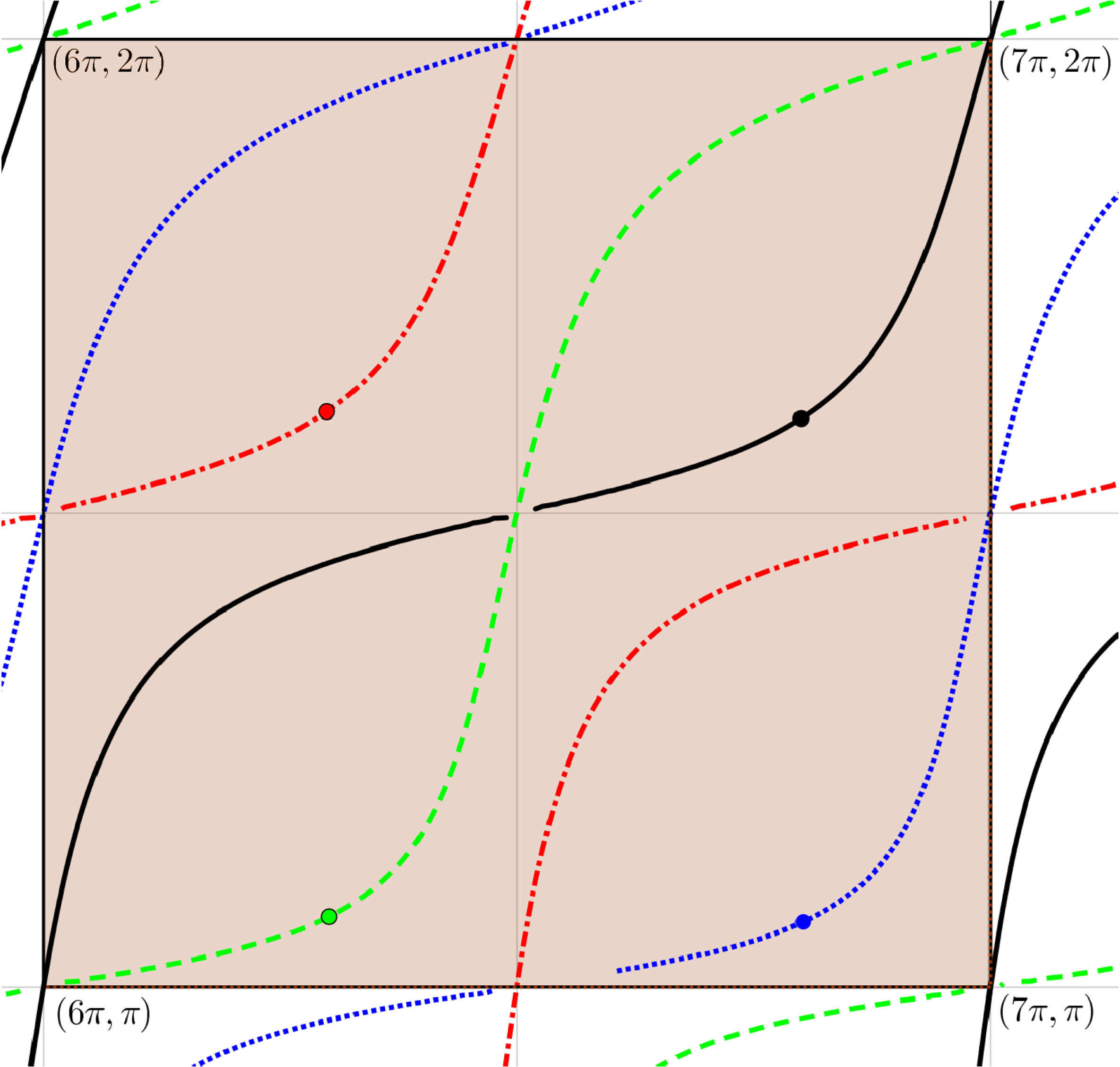
Various $C_{T}$ curves in the situation where $d=3$ , $p=2$ and $\unicode[STIX]{x1D70F}_{1}=\{1,2\}$ .

Figure 3

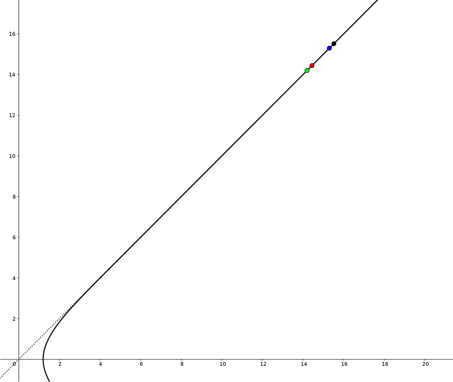
The curve $C_{H}$ corresponding to $\ell (3)=1$ and $\ell (4)=0$ : $x_{3}\tanh (x_{3})=x_{4}\coth (x_{4})$ .

We now turn to assertion (iii). Observe first that there is a uniform bound on $c_{\ell }$ hence there is a $N$ such that if $|\mathbf{n}|>N$ then

$$\begin{eqnarray}\inf _{\mathbf{x}\in I_{\mathbf{n}}}|\mathbf{x}|>c_{\ell }.\end{eqnarray}$$

From the previous discussion this ensures that there are exactly $2^{q}$ solutions in the box $I_{\mathbf{n}}$ . We proceed in two steps for the more quantitative part of the statement. First, we prove that eigenvalues do take the form (2.3.2), and then we show that for all $k\in \{1,2,\ldots ,2^{q}\}$ the same $\boldsymbol{\unicode[STIX]{x1D6FC}}_{\mathbf{n}}$ works.

Localization. Fix the restriction $\ell :\unicode[STIX]{x1D70F}_{2}\rightarrow \{0,1\}^{q}$ for the moment. The various choices of trigonometric factors (represented by the choice of $\ell :\unicode[STIX]{x1D70F}_{1}\rightarrow \{0,1\}^{p}$ ) gives rises to exactly one solution $\boldsymbol{\unicode[STIX]{x1D6FC}}_{2\mathbf{n}+\mathbf{m}}$ in each of the $2^{p}$ boxes $I_{2\mathbf{n}+\mathbf{m}}$ , where $\mathbf{m}$ runs over all choices of $\mathbf{m}\in \{0,1\}^{p}$ . For each of these $\mathbf{m}$ , the corresponding eigenvalue is given by any of the functions appearing in equation (2.3.5) evaluated on any of the coordinates of $(\boldsymbol{\unicode[STIX]{x1D6FC}}_{2\mathbf{n}+\mathbf{m}},\boldsymbol{\unicode[STIX]{x1D6FD}}_{2\mathbf{n}+\mathbf{m}})\in \mathbb{R}^{p}\times \mathbb{R}^{q}$ . It follows that for each $j\in \unicode[STIX]{x1D70F}_{2}$ , and $\mathbf{n}\in \mathbb{N}^{q}$

$$\begin{eqnarray}\displaystyle |\boldsymbol{\unicode[STIX]{x1D6FD}}_{\mathbf{n}}|^{2}=\mathop{\sum }_{i\in \unicode[STIX]{x1D70F}_{2}}\unicode[STIX]{x1D6FD}_{\mathbf{n},i}^{2}=q\unicode[STIX]{x1D6FD}_{\mathbf{n},j}^{2}+O(|\mathbf{n}|^{-\infty }). & & \displaystyle \nonumber\end{eqnarray}$$

Hence for each $j\in \unicode[STIX]{x1D70F}_{2}$ ,

$$\begin{eqnarray}\unicode[STIX]{x1D6FD}_{\mathbf{n},j}=\frac{|\boldsymbol{\unicode[STIX]{x1D6FD}}_{\mathbf{n}}|}{\sqrt{q}}+O(|\mathbf{n}|^{-\infty }).\end{eqnarray}$$

The corresponding eigenvalue is therefore given, for any $j\in \unicode[STIX]{x1D70F}_{2}$ , by

$$\begin{eqnarray}\displaystyle \unicode[STIX]{x1D70E}_{\mathbf{n}}=H_{a_{j},\ell (j)}(\unicode[STIX]{x1D6FD}_{\mathbf{n},j})=\frac{|\boldsymbol{\unicode[STIX]{x1D6FD}}_{\mathbf{n}}|}{\sqrt{q}}+O(|\mathbf{n}|^{-\infty })=\frac{|\boldsymbol{\unicode[STIX]{x1D6FC}}_{\mathbf{n}}|}{\sqrt{q}}+O(|\mathbf{n}|^{-\infty }), & & \displaystyle \nonumber\end{eqnarray}$$

as was announced.

Clustering. If $\ell ,\ell ^{\prime }:S_{d}\rightarrow \{0,1\}$ agree on $\unicode[STIX]{x1D70F}_{1}$ , it follows from

$$\begin{eqnarray}\displaystyle H_{a_{j},\ell (j)}(x)-H_{a_{j},\ell ^{\prime }(j)}(x)=O(x^{-\infty }) & & \displaystyle \nonumber\end{eqnarray}$$

that the corresponding eigenvalues satisfy

$$\begin{eqnarray}\displaystyle \unicode[STIX]{x1D70E}_{\mathbf{n},\ell }-\unicode[STIX]{x1D70E}_{\mathbf{n},\ell ^{\prime }}=O(|\mathbf{n}|^{-\infty }). & & \displaystyle \nonumber\end{eqnarray}$$

The various choices of the restriction $\ell :\unicode[STIX]{x1D70F}_{2}\rightarrow \{0,1\}$ therefore lead to $2^{q}$ eigenvalues satisfying

$$\begin{eqnarray}\unicode[STIX]{x1D70E}_{\mathbf{n}}^{k}=\frac{|\boldsymbol{\unicode[STIX]{x1D6FC}}_{\mathbf{n}}|}{\sqrt{q}}+O(|\mathbf{n}|^{-\infty })\quad \text{for }k=1,\ldots ,2^{q}.\end{eqnarray}$$

Exceptional eigenvalues. For $\mathbf{n}\in \mathbb{N}_{0}^{p}\setminus \mathbb{N}^{p}$ we have that $n_{i}=0$ for at least one $i\in \unicode[STIX]{x1D70F}_{1}$ . On the interval $(0,\unicode[STIX]{x1D70B}/2a_{i}]$ , the function $T_{a_{i},0}$ is positive while $T_{a_{i},1}$ is negative, hence an eigenvalue can only correspond to $\ell (i)=0$ . In this case, the range of $T_{a_{i},0}$ is $[0,a_{i}^{-1})$ . A corresponding eigenvalue is therefore bounded above by $a_{i}^{-1}$ . There is only a finite number of these, proving assertion (iv).

This concludes the proof of Theorem 2.6. ◻

In the next section we will take up the task of understanding the asymptotic behaviour of the counting function $N(\unicode[STIX]{x1D70E})$ .

3.1 A hierarchy of counting functions

Let $p\in \{1,2,\ldots ,d-1\}$ . Given $\unicode[STIX]{x1D70F}=(\unicode[STIX]{x1D70F}_{1},\unicode[STIX]{x1D70F}_{2})\in {\mathcal{T}}_{p}$ and $\ell :S_{d}\rightarrow \{0,1\}$ , define the counting function $N^{\unicode[STIX]{x1D70F},\ell }:\mathbb{R}\rightarrow \mathbb{N}$ by

$$\begin{eqnarray}N^{\unicode[STIX]{x1D70F},\ell }(\unicode[STIX]{x1D70E})=\#\{j\in \mathbb{N}:\unicode[STIX]{x1D70E}_{j}\in S_{\unicode[STIX]{x1D70F},\ell }\text{ and }\unicode[STIX]{x1D70E}_{j}<\unicode[STIX]{x1D70E}\}.\end{eqnarray}$$

Recall that the bipartition $\unicode[STIX]{x1D70F}$ defines the location $\unicode[STIX]{x1D70F}_{1}$ of the trigonometric factors, and the location $\unicode[STIX]{x1D70F}_{2}$ of the hyperbolic factors, whereas the function $\ell$ distinguishes between $\sin$ and $\cos$ trigonometric factors, and $\sinh$ and $\cosh$ hyperbolic factors. We also introduce

(3.1.1) $$\begin{eqnarray}\displaystyle N^{\unicode[STIX]{x1D70F}}(\unicode[STIX]{x1D70E}):=\mathop{\sum }_{\ell :S_{d}\rightarrow \{0,1\}^{d}}N^{\unicode[STIX]{x1D70F},\ell }(\unicode[STIX]{x1D70E})\quad \text{and}\quad N_{p}(\unicode[STIX]{x1D70E}):=\mathop{\sum }_{\unicode[STIX]{x1D70F}\in {\mathcal{T}}_{p}}N^{\unicode[STIX]{x1D70F}}(\unicode[STIX]{x1D70E}). & & \displaystyle\end{eqnarray}$$

Since there is only a finite number of eigenfunctions with linear factors, one has

$$\begin{eqnarray}\displaystyle N(\unicode[STIX]{x1D70E})=\mathop{\sum }_{p=1}^{d-1}N_{p}(\unicode[STIX]{x1D70E})+O(1). & & \displaystyle \nonumber\end{eqnarray}$$

Set $q=d-p$ and let $\unicode[STIX]{x2202}^{q}\unicode[STIX]{x1D6FA}$ denote the union of $p$ -dimensional facets of a cuboid $\unicode[STIX]{x1D6FA}$ . Our goal is to prove the following asymptotics for $N_{p}(\unicode[STIX]{x1D70E})$ .

Proposition 3.1. For each $p=1,\ldots ,d-1$ , we have

(3.1.2) $$\begin{eqnarray}\displaystyle N_{p}(\unicode[STIX]{x1D70E})=\frac{\sqrt{q^{p}}}{(2\unicode[STIX]{x1D70B})^{p}}\unicode[STIX]{x1D714}_{p}\text{Vol}_{p}(\unicode[STIX]{x2202}^{q}\unicode[STIX]{x1D6FA})\unicode[STIX]{x1D70E}^{p}+c_{p}\text{Vol}_{p-1}(\unicode[STIX]{x2202}^{q+1}\unicode[STIX]{x1D6FA})\unicode[STIX]{x1D70E}^{p-1}+O(\unicode[STIX]{x1D70E}^{\unicode[STIX]{x1D702}_{p}}), & & \displaystyle \nonumber\\ \displaystyle & & \displaystyle\end{eqnarray}$$

where $c_{p}$ are some explicitly computable constants and

$$\begin{eqnarray}\displaystyle \unicode[STIX]{x1D702}_{p}=\max \biggl(p-1-\frac{1}{p},p-2+\frac{2}{p+1}\biggr)=\left\{\begin{array}{@{}ll@{}}2/3\quad & \text{if }p=2,\\ p-1-1/p\quad & \text{otherwise}.\end{array}\right. & & \displaystyle \nonumber\end{eqnarray}$$

We prove Proposition 3.1 in §3.5.

3.2 Quasi-eigenvalues

In this section, we observe that the clustering of eigenvalues in Theorem 2.6 allows us to simplify the eigenvalue counting problem. Essentially, we will count every cluster as one eigenvalue with a weight equal to the number of eigenvalues in the cluster.

It is clear from Theorem 2.6 that

(3.2.1) $$\begin{eqnarray}\displaystyle N(\unicode[STIX]{x1D70E})=\mathop{\sum }_{p=1}^{d-1}2^{q}\#\bigg\{\mathbf{n}\in \mathbb{N}^{p}:\frac{|\boldsymbol{\unicode[STIX]{x1D6FC}}_{\mathbf{n}}|}{\sqrt{q}}<\unicode[STIX]{x1D70E}\bigg\}+O(1). & & \displaystyle\end{eqnarray}$$

The factor $2^{q}$ accounts for the clustering of eigenvalues around the corresponding quasi-eigenvalue. Note that the $O(1)$ error can be absorbed in the error term in (1.2.1). Therefore, in view of (3.2.1), for our purposes there is no need to distinguish between counting eigenvalues and quasi-eigenvalues.

3.3 Eigenfunctions with a single trigonometric factor

Consider first the case $p=1$ . The choice of $\sin$ or $\cos$ for the trigonometric factor and the choice of the coordinate corresponding to the trigonometric factor yields $2d$ families of eigenfunctions, each having $2^{d-1}$ possibilities for the choice of the hyperbolic factor. As follows from Theorem 2.6, each of the $2d$ families contributes a cluster of $2^{d-1}$ eigenvalues which correspond to the same quasi-eigenvalue. Therefore, as was mentioned earlier, this cluster can be counted for our purposes as a single quasi-eigenvalue of multiplicity $2^{d-1}$ . The compatibility equations

(3.3.1) $$\begin{eqnarray}\displaystyle H_{a_{i},\ell (i)}(\unicode[STIX]{x1D6FD}_{i})=H_{a_{j},\ell (j)}(\unicode[STIX]{x1D6FD}_{j})\quad \text{for all }i,j\in \unicode[STIX]{x1D70F}_{2} & & \displaystyle\end{eqnarray}$$

define a connected curve in $\mathbb{R}^{d-1}$ which goes to infinity along the diagonal while its value increases to $+\infty$ . Equating (3.3.1) to $T_{a_{k},\ell (k)}$ , $k\in \unicode[STIX]{x1D70F}_{1}$ amounts to solving the following equations:

$$\begin{eqnarray}\displaystyle \unicode[STIX]{x1D6FC}_{k}\cot (a_{k}\unicode[STIX]{x1D6FC}_{k})=\frac{\unicode[STIX]{x1D6FC}_{k}}{\sqrt{d-1}}+O(\unicode[STIX]{x1D6FC}_{k}^{-\infty })\quad \text{if }\ell (k)=0, & & \displaystyle \nonumber\end{eqnarray}$$

and

$$\begin{eqnarray}\displaystyle -\unicode[STIX]{x1D6FC}_{k}\tan (a_{k}\unicode[STIX]{x1D6FC}_{k})=\frac{\unicode[STIX]{x1D6FC}_{k}}{\sqrt{d-1}}+O(\unicode[STIX]{x1D6FC}_{k}^{-\infty })\quad \text{if }\ell (k)=1. & & \displaystyle \nonumber\end{eqnarray}$$

This yields eigenvalues of the form

$$\begin{eqnarray}\displaystyle \unicode[STIX]{x1D70E}=\left\{\begin{array}{@{}ll@{}}\displaystyle \frac{\unicode[STIX]{x1D70B}j}{a_{j}\sqrt{d-1}}+\frac{1}{a_{j}\sqrt{d-1}}\,\text{arccot}((d-1)^{-1/2})+O(j^{-\infty })\quad & \text{if }\ell (k)=0,\\ \displaystyle \frac{\unicode[STIX]{x1D70B}j}{a_{j}\sqrt{d-1}}+\frac{1}{a_{j}\sqrt{d-1}}\arctan ((d-1)^{-1/2})+O(j^{-\infty })\quad & \text{if }\ell (k)=1,\end{array}\right. & & \displaystyle \nonumber\end{eqnarray}$$

each with quasi-multiplicity $2^{d-1}$ . Given that $\text{arccot}$ and $\arctan$ are bounded functions, and since

$$\begin{eqnarray}\displaystyle \text{Vol}_{1}(\unicode[STIX]{x2202}^{d-1}\unicode[STIX]{x1D6FA})=2^{d}\mathop{\sum }_{j=1}^{d}a_{j}, & & \displaystyle \nonumber\end{eqnarray}$$

we have that

$$\begin{eqnarray}\displaystyle N_{1}(\unicode[STIX]{x1D70E})=\frac{\unicode[STIX]{x1D714}_{1}\sqrt{d-1}}{2\unicode[STIX]{x1D70B}}\text{Vol}_{1}(\unicode[STIX]{x2202}^{d-1}\unicode[STIX]{x1D6FA})\unicode[STIX]{x1D70E}+O(1). & & \displaystyle \nonumber\end{eqnarray}$$

This concludes the proof of Theorem  1.1 for $d=2$ , since $p=1$ is the only possibility in this case. Observe that for $d=2$ , this is indeed the expected first term of Weyl’s law (1.1.2).

3.4 Eigenfunctions with many trigonometric factors

In this subsection, we count the number of eigenvalues associated with eigenfunctions with more than one trigonometric factor. The idea is to write the eigenvalues as the norms of points $\boldsymbol{\unicode[STIX]{x1D6FC}}\in \mathbb{R}^{p}$ that are close to some lattice points. The main difficulty is that the compatibility equations are transcendental, making it impossible to explicitly find $\boldsymbol{\unicode[STIX]{x1D6FC}}$ . We will therefore approximate the eigenvalues in a controlled way, and we will show that this approximation results in a small enough error that could be absorbed in the remainder in the two-term asymptotics for the eigenvalue counting function. Finally, we will use the lattice point counting techniques going back to [Reference Hlawka8, Reference Randol15], and more recently used in [Reference Lagacé and Parnovski11].

3.4.1 Approximate eigenvalues

Suppose that $d\geqslant 3$ and $p\in \{2,\ldots ,d-1\}$ . Let $\unicode[STIX]{x1D70F}\in {\mathcal{T}}_{p}$ and $\ell :S_{d}\rightarrow \{0,1\}$ be given.

Given $\mathbf{n}\in \mathbb{N}^{p}$ , it follows from Theorem 2.6 and the compatibility equations (2.2.3), that the corresponding solution $\boldsymbol{\unicode[STIX]{x1D6FC}}=\boldsymbol{\unicode[STIX]{x1D6FC}}_{\mathbf{n}}\in I_{\mathbf{n}}$ satisfies the following for each $i,j\in \unicode[STIX]{x1D70F}_{1}$ :

$$\begin{eqnarray}\displaystyle \unicode[STIX]{x1D6FC}_{i}\cot \biggl(\unicode[STIX]{x1D6FC}_{i}a_{i}+\frac{\ell (i)\unicode[STIX]{x1D70B}}{2}\biggr)=\unicode[STIX]{x1D6FC}_{j}\cot \biggl(\unicode[STIX]{x1D6FC}_{j}a_{j}+\frac{\ell (j)\unicode[STIX]{x1D70B}}{2}\biggr)=\frac{|\boldsymbol{\unicode[STIX]{x1D6FC}}_{\mathbf{n}}|}{\sqrt{q}}+O(|\mathbf{n}|^{-\infty }). & & \displaystyle \nonumber\end{eqnarray}$$

Hence, for each $i\in \unicode[STIX]{x1D70F}_{1}$ , we have, choosing the principal branch of $\text{arccot}$ , a family of solutions indexed by $\mathbf{n}\in \mathbb{N}^{p}$

$$\begin{eqnarray}\displaystyle \unicode[STIX]{x1D6FC}_{i}a_{i}=\biggl(n_{i}+\frac{\ell (i)}{2}\biggr)\unicode[STIX]{x1D70B}+\text{arccot}\biggl(\frac{1}{\sqrt{q}}\biggl[1+\mathop{\sum }_{j\neq i\in \unicode[STIX]{x1D70F}_{1}}\biggl(\frac{\unicode[STIX]{x1D6FC}_{j}}{\unicode[STIX]{x1D6FC}_{i}}\biggr)^{2}\biggr]^{1/2}\biggr)+O(|\mathbf{n}|^{-\infty }). & & \displaystyle \nonumber\end{eqnarray}$$

Since $\unicode[STIX]{x1D6FC}_{i}=(n_{i}+\ell (i)/2)\unicode[STIX]{x1D70B}/a_{i}+O(1)$ , we can rewrite the previous equation as follows:

(3.4.1) $$\begin{eqnarray}\displaystyle \unicode[STIX]{x1D6FC}_{i} & = & \displaystyle \frac{(n_{i}+\ell (i)/2)\unicode[STIX]{x1D70B}}{a_{i}}\nonumber\\ \displaystyle & & \displaystyle +\,\frac{1}{a_{i}}\,\text{arccot}\biggl(\frac{1}{\sqrt{q}}\biggl[1+\mathop{\sum }_{j\neq i}\biggl(\frac{(n_{\!j}+\ell (j)/2)\unicode[STIX]{x1D70B}/a_{j}+t_{\unicode[STIX]{x1D6FC}_{j}}(\mathbf{n})}{(n_{i}+\ell (i)/2)\unicode[STIX]{x1D70B}/a_{i}+t_{\unicode[STIX]{x1D6FC}_{i}}(\mathbf{n})}\biggr)^{2}\biggr]^{1/2}\biggr)\nonumber\\ \displaystyle & & \displaystyle +\,O(|\mathbf{n}|^{-\infty }),\end{eqnarray}$$

where the functions $t_{\unicode[STIX]{x1D6FC}_{j}}$ are bounded. Since $\ell (i)$ ranges over $\{0,1\}$ , the solution set to the previous equation is the same as the one to

(3.4.2) $$\begin{eqnarray}\displaystyle \unicode[STIX]{x1D6FC}_{i}=\frac{n_{i}\unicode[STIX]{x1D70B}}{2a_{i}}+\frac{1}{a_{i}}\,\text{arccot}\biggl(\frac{1}{\sqrt{q}}\biggl[1+\mathop{\sum }_{j\neq i}\biggl(\frac{n_{\!j}\unicode[STIX]{x1D70B}/2a_{j}+t_{\unicode[STIX]{x1D6FC}_{j}}(\mathbf{n})}{n_{i}\unicode[STIX]{x1D70B}/2a_{i}+t_{\unicode[STIX]{x1D6FC}_{i}}(\mathbf{n})}\biggr)^{2}\biggr]^{1/2}\biggr)+O(|\mathbf{n}|^{-\infty }). & & \displaystyle \nonumber\\ \displaystyle & & \displaystyle\end{eqnarray}$$

Lemma 3.3. Define $\widetilde{\unicode[STIX]{x1D6FC}}_{i}$ as

(3.4.3) $$\begin{eqnarray}\displaystyle \widetilde{\unicode[STIX]{x1D6FC}}_{i}=\frac{n_{i}\unicode[STIX]{x1D70B}}{2a_{i}}+\frac{1}{a_{i}}\,\text{arccot}\biggl(\frac{1}{\sqrt{q}}\biggl[1+\mathop{\sum }_{j\neq i}\biggl(\frac{a_{i}n_{\!j}}{a_{j}n_{i}}\biggr)^{2}\biggr]^{1/2}\biggr). & & \displaystyle\end{eqnarray}$$

Then

(3.4.4) $$\begin{eqnarray}\displaystyle \widetilde{\unicode[STIX]{x1D6FC}}_{i}=\unicode[STIX]{x1D6FC}_{i}+O(|\mathbf{n}|^{-1}). & & \displaystyle\end{eqnarray}$$

Proof. In Lemma A.1 in the Appendix, take $x_{i}=n_{i}\unicode[STIX]{x1D70B}/a_{i}$ and $\unicode[STIX]{x1D713}_{i}=t_{\unicode[STIX]{x1D6FC}_{i}}$ . Then one readily sees that

$$\begin{eqnarray}|\mathbf{x}|\asymp |\mathbf{n}|,\end{eqnarray}$$

where $f\asymp g$ means that $f=O(g)$ and $g=O(f)$ . The lemma then follows.◻

Note that the right-hand side of equation (3.4.3) does not depend on $\unicode[STIX]{x1D6FC}_{i}$ anymore, which makes it easier to analyse.

We now have eigenvalues indexed by $\mathbf{n}\in \mathbb{N}^{p}$ given by

(3.4.5) $$\begin{eqnarray}\displaystyle \unicode[STIX]{x1D70E}_{\mathbf{n}}=\sqrt{\frac{1}{q}\mathop{\sum }_{i\in \unicode[STIX]{x1D70F}_{1}}\widetilde{\unicode[STIX]{x1D6FC}}_{i}^{2}}+O(|\mathbf{n}|^{-1}). & & \displaystyle\end{eqnarray}$$

Definition 3.4. The numbers

(3.4.6) $$\begin{eqnarray}\displaystyle \widetilde{\unicode[STIX]{x1D70E}}_{\mathbf{n}}=\sqrt{\frac{1}{q}\mathop{\sum }_{i\in \unicode[STIX]{x1D70F}_{1}}\widetilde{\unicode[STIX]{x1D6FC}}_{i}^{2}} & & \displaystyle\end{eqnarray}$$

are called the approximate eigenvalues.

Remark 3.5. Up until now, eigenvalues, quasi-eigenvalues and approximate eigenvalues were indexed by $\mathbf{n}\in \mathbb{N}^{p}$ . In the following two theorems it is convenient to use $n\in \mathbb{N}$ to index them in ascending order.

The following lemma allows us to estimate the error induced by counting approximate eigenvalues instead of eigenvalues.

Lemma 3.6. Let $(a_{n}),(b_{n})$ be two sequences of positive numbers which tend to infinity. Suppose there exists a number $s>-1$ such that $a_{n}=b_{n}+O(b_{n}^{-s})$ . Let

$$\begin{eqnarray}\displaystyle N_{a}(\unicode[STIX]{x1D706})=\#\{n:a_{n}<\unicode[STIX]{x1D706}\}\quad \text{and}\quad N_{b}(\unicode[STIX]{x1D706})=\#\{n:b_{n}<\unicode[STIX]{x1D706}\}. & & \displaystyle \nonumber\end{eqnarray}$$

Suppose that there exists a number $K$ such that

$$\begin{eqnarray}\displaystyle N_{a}(\unicode[STIX]{x1D706})=\mathop{\sum }_{k=0}^{K}c_{k}\unicode[STIX]{x1D706}^{p-k}+O(\unicode[STIX]{x1D706}^{r}), & & \displaystyle \nonumber\end{eqnarray}$$

with $r<p-K$ . Then

(3.4.7) $$\begin{eqnarray}\displaystyle N_{b}(\unicode[STIX]{x1D706})=\mathop{\sum }_{k=0}^{K}c_{k}\unicode[STIX]{x1D706}^{p-k}+O(\unicode[STIX]{x1D706}^{r^{\prime }}), & & \displaystyle\end{eqnarray}$$

where $r^{\prime }=\max (r,p-1-s)$ .

Remark 3.7. Note that if $r^{\prime }\geqslant p-K$ , some of the terms in the sum in (3.4.7) might be absorbed in the error term.

Proof. Indeed, the assumption on the sequences $a_{n}$ and $b_{n}$ implies that there exists $c>0$ such that

$$\begin{eqnarray}\displaystyle N_{a}\biggl(\unicode[STIX]{x1D706}+\frac{c}{\unicode[STIX]{x1D706}^{s}}\biggr)\leqslant N_{b}(\unicode[STIX]{x1D706})\leqslant N_{a}\biggl(\unicode[STIX]{x1D706}-\frac{c}{\unicode[STIX]{x1D706}^{s}}\biggr). & & \displaystyle \nonumber\end{eqnarray}$$

A direct computation of $N_{a}(\unicode[STIX]{x1D706}\pm c\unicode[STIX]{x1D706}^{-s})$ completes the proof of the lemma.◻

Recall now the definition of $N^{\unicode[STIX]{x1D70F}}(\unicode[STIX]{x1D70E})$ given by (3.1.1). We will write $\widetilde{N}^{\unicode[STIX]{x1D70F}}$ for the counting function of the corresponding approximate eigenvalues.

Lemma 3.8. We have

$$\begin{eqnarray}\displaystyle |\widetilde{N}^{\unicode[STIX]{x1D70F}}(\unicode[STIX]{x1D70E})-N^{\unicode[STIX]{x1D70F}}(\unicode[STIX]{x1D70E})|=O(\unicode[STIX]{x1D70E}^{p-1-1/p}). & & \displaystyle \nonumber\end{eqnarray}$$

Proof. Both the eigenvalues and the approximate eigenvalues are, up to a bounded error, the norms of the points of the lattice $\unicode[STIX]{x1D6E4}=\bigoplus _{i=1}^{p}(\unicode[STIX]{x1D70B}/2a_{i}\sqrt{q})\mathbb{N}$ , repeated $2^{q}$ times. Denote by $l_{n}:=\{|\boldsymbol{\unicode[STIX]{x1D6FE}}|:\boldsymbol{\unicode[STIX]{x1D6FE}}\in \unicode[STIX]{x1D6E4}\}_{n}$ the sequence of norms of the points of the lattice $\unicode[STIX]{x1D6E4}$ arranged in ascending order. It is well known that there is a constant $C$ such that

$$\begin{eqnarray}\displaystyle N_{l}(\unicode[STIX]{x1D70E})=C\unicode[STIX]{x1D70E}^{p}+O(\unicode[STIX]{x1D70E}^{p-1}), & & \displaystyle \nonumber\end{eqnarray}$$

where $C$ depends on $\unicode[STIX]{x1D6E4}$ and $N_{l}$ denotes the counting function of the sequence $l_{n}$ as in Lemma 3.6. Applying Lemma 3.6 with $s=0$ yields

$$\begin{eqnarray}\displaystyle N^{\unicode[STIX]{x1D70F}}(\unicode[STIX]{x1D70E})=2^{q}C\unicode[STIX]{x1D70E}^{p}+O(\unicode[STIX]{x1D70E}^{p-1}). & & \displaystyle \nonumber\end{eqnarray}$$

Reversing this expression tells us that

(3.4.8) $$\begin{eqnarray}\displaystyle \unicode[STIX]{x1D70E}_{n}=\biggl(\frac{n}{2^{q}C}\biggr)^{1/p}+o(n^{1/p}). & & \displaystyle\end{eqnarray}$$

From equations (3.4.6) and (3.4.8) we have that

$$\begin{eqnarray}\displaystyle \widetilde{\unicode[STIX]{x1D70E}}_{n}=\unicode[STIX]{x1D70E}_{n}+O(n^{-1/p}). & & \displaystyle \nonumber\end{eqnarray}$$

Therefore, applying once again Lemma 3.6, but this time with $s=1/p$ , yields

(3.4.9) $$\begin{eqnarray}\displaystyle N^{\unicode[STIX]{x1D70F}}(\unicode[STIX]{x1D70E})=\widetilde{N}^{\unicode[STIX]{x1D70F}}(\unicode[STIX]{x1D70E})+O(\unicode[STIX]{x1D70E}^{p-1-1/p}). & & \displaystyle\end{eqnarray}$$

◻

3.4.2 Another representation of the counting function

For every $\unicode[STIX]{x1D70F}$ , let us now define a family of sets $E_{\unicode[STIX]{x1D70E}}\subset \mathbb{R}^{p}$ with the property that

(3.4.10) $$\begin{eqnarray}\displaystyle \widetilde{N}^{\unicode[STIX]{x1D70F}}(\unicode[STIX]{x1D70E})=\mathop{\sum }_{\mathbf{n}\in \mathbb{N}^{p}}2^{q}\unicode[STIX]{x1D712}\biggl(\frac{\mathbf{n}}{\unicode[STIX]{x1D70E}}\biggr)+O(1), & & \displaystyle\end{eqnarray}$$

where $\unicode[STIX]{x1D712}:=\unicode[STIX]{x1D712}_{\unicode[STIX]{x1D70E}}$ is the indicator function of $E_{\unicode[STIX]{x1D70E}}$ . Let us define elliptic polar coordinates in $\mathbb{R}^{p}$ with the convention that $\unicode[STIX]{x1D703}_{p}=0$ :

(3.4.11) $$\begin{eqnarray}\displaystyle \begin{array}{@{}rcl@{}}r^{2}\; & =\; & \displaystyle \mathop{\sum }_{i\in \unicode[STIX]{x1D70F}_{1}}\biggl(\frac{\unicode[STIX]{x1D70B}x_{i}}{2a_{i}\sqrt{q}}\biggr)^{2},\\ x_{\!j}\; & =\; & \displaystyle r\frac{2a_{j}\sqrt{q}}{\unicode[STIX]{x1D70B}}\cos (\unicode[STIX]{x1D703}_{j})\mathop{\prod }_{i<j}\sin (\unicode[STIX]{x1D703}_{i}).\end{array} & & \displaystyle\end{eqnarray}$$

We define the family of sets

(3.4.12) $$\begin{eqnarray}\displaystyle E_{\unicode[STIX]{x1D70E}}:=\bigg\{(r,\boldsymbol{\unicode[STIX]{x1D703}})\in \mathbb{R}^{p}:r^{2}+\frac{2r}{\unicode[STIX]{x1D70E}}\mathop{\sum }_{j\in \unicode[STIX]{x1D70F}_{1}}\frac{1}{a_{j}}g_{j}(\boldsymbol{\unicode[STIX]{x1D703}})+\frac{H(\boldsymbol{\unicode[STIX]{x1D703}})}{\unicode[STIX]{x1D70E}^{2}}<1\bigg\},\qquad & & \displaystyle\end{eqnarray}$$

with

(3.4.13) $$\begin{eqnarray}\displaystyle g_{j}(\boldsymbol{\unicode[STIX]{x1D703}}):=\cos \unicode[STIX]{x1D703}_{j}\mathop{\prod }_{i<j}\sin \unicode[STIX]{x1D703}_{i}\,\text{arccot}\biggl(\frac{1}{\sqrt{q}}\biggl[1+\mathop{\sum }_{i\neq j}\biggl(\frac{x_{i}}{x_{\!j}}\biggr)^{2}\biggr]^{1/2}\biggr),\qquad & & \displaystyle\end{eqnarray}$$

and

$$\begin{eqnarray}\displaystyle H=H(\boldsymbol{\unicode[STIX]{x1D703}})=\mathop{\sum }_{j\in \unicode[STIX]{x1D70F}_{1}}\frac{1}{a_{j}^{2}}\,\text{arccot}\biggl(\frac{1}{\sqrt{q}}\biggl[1+\mathop{\sum }_{i\neq j}\biggl(\frac{x_{i}}{x_{\!j}}\biggr)^{2}\biggr]^{1/2}\biggr)^{2}. & & \displaystyle \nonumber\end{eqnarray}$$

From equation (3.4.6), we can observe that the evaluation of $\unicode[STIX]{x1D712}$ at $\unicode[STIX]{x1D70E}^{-1}\mathbf{n}$ in coordinates (3.4.11) is $1$ if and only if $\widetilde{\unicode[STIX]{x1D70E}}_{\mathbf{n}}<\unicode[STIX]{x1D70E}$ . If $|\mathbf{n}|>N$ as in Theorem 2.6, there are $2^{q}$ solutions close to any order to $\widetilde{\unicode[STIX]{x1D70E}}_{\mathbf{n}}$ . This achieves our stated goal of equation (3.4.10). Let us now prove a few properties of the set $E_{\unicode[STIX]{x1D70E}}$ that will be required in the sequel.

Lemma 3.9. There exists $\unicode[STIX]{x1D70E}_{0}$ , such that for $\unicode[STIX]{x1D70E}>\unicode[STIX]{x1D70E}_{0}$ the set $E_{\unicode[STIX]{x1D70E}}$ is strictly convex and the principal curvatures of $\unicode[STIX]{x2202}E_{\unicode[STIX]{x1D70E}}$ are positive and uniformly bounded away from $0$ . Furthermore, the boundary $\unicode[STIX]{x2202}E_{\unicode[STIX]{x1D70E}}$ is smooth for all $\unicode[STIX]{x1D70E}>\unicode[STIX]{x1D70E}_{0}$ , and all the derivatives of the boundary defining function are uniformly bounded in $\unicode[STIX]{x1D70E}>\unicode[STIX]{x1D70E}_{0}$ .

Proof. From equation (3.4.12) $\unicode[STIX]{x2202}E_{\unicode[STIX]{x1D70E}}$ is the level set of the function

$$\begin{eqnarray}F(r,\boldsymbol{\unicode[STIX]{x1D703}})=r^{2}+\frac{2r}{\unicode[STIX]{x1D70E}}\mathop{\sum }_{j\in \unicode[STIX]{x1D70F}_{1}}\frac{1}{a_{j}}g_{j}(\boldsymbol{\unicode[STIX]{x1D703}})+\frac{H(\boldsymbol{\unicode[STIX]{x1D703}})}{\unicode[STIX]{x1D70E}^{2}},\end{eqnarray}$$

which satisfies

(3.4.14) $$\begin{eqnarray}\displaystyle \begin{array}{@{}rcl@{}}F(r,\boldsymbol{\unicode[STIX]{x1D703}})\; & =\; & r^{2}+O(\unicode[STIX]{x1D70E}^{-1}),\\ \text{}[\unicode[STIX]{x1D6FB}F(\mathbf{x})]_{i}\; & =\; & \displaystyle \frac{\unicode[STIX]{x1D70B}x_{i}}{a_{i}\sqrt{q}}+O(\unicode[STIX]{x1D70E}^{-1}),\\ \operatorname{Hess}F\; & =\; & \text{diag}\biggl(\displaystyle \frac{\unicode[STIX]{x1D70B}}{a_{i}\sqrt{q}}\biggr)_{i\in \unicode[STIX]{x1D70F}_{1}}+O(\unicode[STIX]{x1D70E}^{-1}).\end{array} & & \displaystyle\end{eqnarray}$$

One can observe that $H$ and $g_{j},j\in \unicode[STIX]{x1D70F}_{1}$ are all smooth functions of $\boldsymbol{\unicode[STIX]{x1D703}}\in \mathbb{S}^{p-1}$ . This automatically yields the claim on the smoothness and the uniform boundedness of the derivatives of the boundary defining function.

Furthermore, for $\unicode[STIX]{x1D70E}$ large enough, the second fundamental form of $\unicode[STIX]{x2202}E_{\unicode[STIX]{x1D70E}}$ , being a positive multiple of $\text{Hess}\,F$ , is positive, with its smallest eigenvalue uniformly bounded away from $0$ . This implies the claim on the principal curvatures, which in turn yields strict convexity of $E_{\unicode[STIX]{x1D70E}}$ .◻

This directly implies the following corollary.

Corollary 3.10. The product of the principal curvatures of $\unicode[STIX]{x2202}E_{\unicode[STIX]{x1D70E}}$ is uniformly bounded away from zero for $\unicode[STIX]{x1D70E}$ large enough.

3.4.3 Poisson summation formula

In this section, we use the general scheme of the proof of [Reference Lagacé and Parnovski11, Theorem 1.1]. Recall that

(3.4.15) $$\begin{eqnarray}\displaystyle N^{\unicode[STIX]{x1D70F}}(\unicode[STIX]{x1D70E}) & = & \displaystyle \mathop{\sum }_{\mathbf{n}\in \mathbb{N}^{p}}2^{q}\unicode[STIX]{x1D712}\biggl(\frac{\mathbf{n}}{\unicode[STIX]{x1D70E}}\biggr)+O(1)\nonumber\\ \displaystyle & = & \displaystyle 2^{q-p}\mathop{\sum }_{\mathbf{n}\in \mathbb{Z}^{p}}\unicode[STIX]{x1D712}\biggl(\frac{\mathbf{n}}{\unicode[STIX]{x1D70E}}\biggr)+R_{\unicode[STIX]{x1D70F}}(\unicode[STIX]{x1D70E})+O(1),\end{eqnarray}$$

where $R_{\unicode[STIX]{x1D70F}}(\unicode[STIX]{x1D70E})$ is the error term induced by the overcounting of points on hyperplanes with one vanishing coordinate.

Our goal is now to compute the terms appearing in equation (3.4.15) using the Poisson summation formula which states, under sufficient smoothness assumptions, that

(3.4.16) $$\begin{eqnarray}\displaystyle \mathop{\sum }_{\mathbf{n}\in \mathbb{Z}^{p}}f(\mathbf{n})=\mathop{\sum }_{\mathbf{m}\in \mathbb{Z}^{p}}\widehat{f}(\mathbf{m}), & & \displaystyle\end{eqnarray}$$

where the Fourier transform is given by

$$\begin{eqnarray}\displaystyle \widehat{f}(\boldsymbol{\unicode[STIX]{x1D709}}):=\int _{\mathbb{R}^{p}}f(\mathbf{x})\text{e}^{-2\unicode[STIX]{x1D70B}\text{i}\mathbf{x}\cdot \boldsymbol{\unicode[STIX]{x1D709}}}\,d\mathbf{x}. & & \displaystyle \nonumber\end{eqnarray}$$

However, $\unicode[STIX]{x1D712}$ is not regular enough for us to use the Poisson summation formula, hence we need to mollify it. Let us introduce a non-negative function $\unicode[STIX]{x1D713}\in C_{c}^{\infty }(\mathbb{R})$ supported in $[-1,1]$ and such that

$$\begin{eqnarray}\displaystyle \int _{0}^{\infty }\unicode[STIX]{x1D713}(r)r^{p-1}\,dr=\frac{1}{V_{p-1}}, & & \displaystyle \nonumber\end{eqnarray}$$

with $V_{p-1}$ being the volume of the $(p-1)$ -dimensional unit sphere in $\mathbb{R}^{p}$ . We then define a family $\unicode[STIX]{x1D6F9}_{\unicode[STIX]{x1D716}}:\mathbb{R}^{p}\rightarrow \mathbb{R}$ of radial bump functions of total mass $1$ by

$$\begin{eqnarray}\displaystyle \unicode[STIX]{x1D6F9}_{\unicode[STIX]{x1D716}}(\mathbf{x})=\frac{1}{\unicode[STIX]{x1D716}^{p}}\unicode[STIX]{x1D713}\biggl(\frac{|\mathbf{x}|}{\unicode[STIX]{x1D716}}\biggr). & & \displaystyle \nonumber\end{eqnarray}$$

Set $\unicode[STIX]{x1D6F9}:=\unicode[STIX]{x1D6F9}_{1}$ Consider the smooth function $\unicode[STIX]{x1D712}_{\unicode[STIX]{x1D716}}=\unicode[STIX]{x1D6F9}_{\unicode[STIX]{x1D716}}\ast \unicode[STIX]{x1D712}$ . Note that

$$\begin{eqnarray}\displaystyle \widehat{\unicode[STIX]{x1D6F9}}_{\unicode[STIX]{x1D716}}(\boldsymbol{\unicode[STIX]{x1D709}})=\widehat{\unicode[STIX]{x1D6F9}}(\unicode[STIX]{x1D716}\boldsymbol{\unicode[STIX]{x1D709}}). & & \displaystyle \nonumber\end{eqnarray}$$

We now prove the following lemma.

Lemma 3.11. Let $\unicode[STIX]{x1D712}_{\unicode[STIX]{x1D716}}^{+},\unicode[STIX]{x1D712}_{\unicode[STIX]{x1D716}}^{-}:\mathbb{R}^{p}\rightarrow \mathbb{R}$ be defined by

$$\begin{eqnarray}\displaystyle \unicode[STIX]{x1D712}_{\unicode[STIX]{x1D716}}^{+}(\mathbf{x}) & = & \displaystyle \unicode[STIX]{x1D712}_{\unicode[STIX]{x1D716}}((1-\unicode[STIX]{x1D702}_{+}\unicode[STIX]{x1D716})\mathbf{x}),\nonumber\\ \displaystyle \unicode[STIX]{x1D712}_{\unicode[STIX]{x1D716}}^{-}(\mathbf{x}) & = & \displaystyle \unicode[STIX]{x1D712}_{\unicode[STIX]{x1D716}}((1+\unicode[STIX]{x1D702}_{-}\unicode[STIX]{x1D716})\mathbf{x})\nonumber\end{eqnarray}$$

for some $\unicode[STIX]{x1D702}_{-},\unicode[STIX]{x1D702}_{+}>0$ . One can choose $\unicode[STIX]{x1D702}_{-},\unicode[STIX]{x1D702}_{+}$ in such a way that for all $\unicode[STIX]{x1D70E}$ large enough

$$\begin{eqnarray}\displaystyle \unicode[STIX]{x1D712}_{\unicode[STIX]{x1D716}}^{-}(\mathbf{x})\leqslant \unicode[STIX]{x1D712}(\mathbf{x})\leqslant \unicode[STIX]{x1D712}_{\unicode[STIX]{x1D716}}^{+}(\mathbf{x}) & & \displaystyle \nonumber\end{eqnarray}$$

for all $\mathbf{x}\in \mathbb{R}^{p}$ and all $\unicode[STIX]{x1D716}>0$ small enough.

Proof. For the first inequality, observe that

$$\begin{eqnarray}\displaystyle \unicode[STIX]{x1D712}_{\unicode[STIX]{x1D716}}((1+\unicode[STIX]{x1D702}_{-}\unicode[STIX]{x1D716})\mathbf{x}) & = & \displaystyle \int _{\mathbb{R}^{p}}\unicode[STIX]{x1D712}(\mathbf{y})\unicode[STIX]{x1D6F9}_{\unicode[STIX]{x1D716}}((1+\unicode[STIX]{x1D702}_{-}\unicode[STIX]{x1D716})\mathbf{x}-\mathbf{y})\,d\mathbf{y}\nonumber\\ \displaystyle & = & \displaystyle \int _{B_{(1+\unicode[STIX]{x1D702}_{-}\unicode[STIX]{x1D716})\mathbf{x}}(\unicode[STIX]{x1D716})}\unicode[STIX]{x1D712}(\mathbf{y})\unicode[STIX]{x1D6F9}_{\unicode[STIX]{x1D716}}((1+\unicode[STIX]{x1D702}_{-}\unicode[STIX]{x1D716})\mathbf{x}-\mathbf{y})\,d\mathbf{y}\nonumber\\ \displaystyle & {\leqslant} & \displaystyle \sup _{B_{(1+\unicode[STIX]{x1D702}_{-}\unicode[STIX]{x1D716})\mathbf{x}}(\unicode[STIX]{x1D716})}\unicode[STIX]{x1D712}(\mathbf{y}).\nonumber\end{eqnarray}$$

Hence, to show that $\unicode[STIX]{x1D712}_{\unicode[STIX]{x1D716}}((1+\unicode[STIX]{x1D702}_{-}\unicode[STIX]{x1D716})\mathbf{x})\leqslant \unicode[STIX]{x1D712}(\mathbf{x})$ for all $\mathbf{x}$ , by convexity of $E_{\unicode[STIX]{x1D70E}}$ it is sufficient to show that for all $\mathbf{x}\in \unicode[STIX]{x2202}E_{\unicode[STIX]{x1D70E}}$ , there exists $\unicode[STIX]{x1D702}_{-}$ , independent of $\unicode[STIX]{x1D70E}$ such that the following holds for each $\unicode[STIX]{x1D716}>0$ small enough

$$\begin{eqnarray}\displaystyle B_{(1+\unicode[STIX]{x1D702}_{-}\unicode[STIX]{x1D716})\mathbf{x}}(\unicode[STIX]{x1D716})\cap E_{\unicode[STIX]{x1D70E}}=\varnothing . & & \displaystyle \nonumber\end{eqnarray}$$

Note that for all $\mathbf{x}\in \unicode[STIX]{x2202}E_{\unicode[STIX]{x1D70E}}$ we have that

(3.4.17) $$\begin{eqnarray}\displaystyle \text{dist}((1+t)\mathbf{x},\unicode[STIX]{x2202}E_{\unicode[STIX]{x1D70E}})=(\mathbf{x}\cdot {\mathcal{N}}_{\unicode[STIX]{x2202}E_{\unicode[STIX]{x1D70E}}}(\mathbf{x}))t+O(t^{2}), & & \displaystyle\end{eqnarray}$$

where ${\mathcal{N}}_{\unicode[STIX]{x2202}E_{\unicode[STIX]{x1D70E}}}$ is the Gauss map of the boundary. To see this, denote by $T_{\mathbf{x}}\unicode[STIX]{x2202}E_{\unicode[STIX]{x1D70E}}$ the tangent hyperplane of $\unicode[STIX]{x2202}E_{\unicode[STIX]{x1D70E}}$ at $\mathbf{x}$ , and by $P_{\mathbf{x}}$ the orthogonal projection on that hyperplane. We have by the triangle inequality that

$$\begin{eqnarray}|\text{dist}((1+t)\mathbf{x},\unicode[STIX]{x2202}E_{\unicode[STIX]{x1D70E}})-\text{dist}((1+t)\mathbf{x},T_{\mathbf{x}}\unicode[STIX]{x2202}E_{\unicode[STIX]{x1D70E}})|\leqslant \text{dist}(P_{\mathbf{x}}((1+t)\mathbf{x}),\unicode[STIX]{x2202}E_{\unicode[STIX]{x1D70E}}).\end{eqnarray}$$

We observe that $\text{dist}((1+t)\mathbf{x},T_{\mathbf{x}}\unicode[STIX]{x2202}E_{\unicode[STIX]{x1D70E}})=(\mathbf{x}\cdot {\mathcal{N}}_{\unicode[STIX]{x2202}E_{\unicode[STIX]{x1D70E}}}(\mathbf{x}))t$ . Let $F$ , as before, be the function in $\mathbb{R}^{p}$ such that the set $F\equiv 1$ coincides with $\unicode[STIX]{x2202}E_{\unicode[STIX]{x1D70E}}$ . Taking the Taylor expansion of $F$ around $\mathbf{x}$ , we have that

$$\begin{eqnarray}\text{dist}(P_{\mathbf{x}}((1+t)\mathbf{x}),\unicode[STIX]{x2202}E_{\unicode[STIX]{x1D70E}})\leqslant \Vert \text{Hess}\,F(\mathbf{x})\Vert _{\infty }|P_{\mathbf{x}}((1+t)\mathbf{x})|^{2}=O(t^{2}),\end{eqnarray}$$

where we used that $\Vert \text{Hess}\,F(\mathbf{x})\Vert _{\infty }$ is bounded uniformly for $\unicode[STIX]{x1D70E}>\unicode[STIX]{x1D70E}_{0}$ and $\mathbf{x}\in \unicode[STIX]{x2202}E_{\unicode[STIX]{x1D70E}}$ . Note that the strict convexity of $\unicode[STIX]{x2202}E_{\unicode[STIX]{x1D70E}}$ and equation (3.4.14) imply that $\mathbf{x}\cdot {\mathcal{N}}_{\unicode[STIX]{x2202}E_{\unicode[STIX]{x1D70E}}}(\mathbf{x})$ is bounded away from zero uniformly for $\unicode[STIX]{x1D70E}>\unicode[STIX]{x1D70E}_{0}$ . This implies that we can choose $\unicode[STIX]{x1D702}_{-}$ large enough and independent in $\unicode[STIX]{x1D70E}$ such that indeed

$$\begin{eqnarray}\displaystyle B_{(1+\unicode[STIX]{x1D702}_{-}\unicode[STIX]{x1D716})\mathbf{x}}(\unicode[STIX]{x1D716})\cap E_{\unicode[STIX]{x1D70E}}=\varnothing . & & \displaystyle \nonumber\end{eqnarray}$$

For the second inequality, we have

$$\begin{eqnarray}\displaystyle \unicode[STIX]{x1D712}_{\unicode[STIX]{x1D716}}((1-\unicode[STIX]{x1D702}_{+}\unicode[STIX]{x1D716})\mathbf{x}) & = & \displaystyle \int _{\mathbb{R}^{p}}\unicode[STIX]{x1D712}(\mathbf{y})\unicode[STIX]{x1D6F9}_{\unicode[STIX]{x1D716}}((1-\unicode[STIX]{x1D702}_{+}\unicode[STIX]{x1D716})\mathbf{x}-\mathbf{y})\,d\mathbf{y}\nonumber\\ \displaystyle & = & \displaystyle \int _{B_{(1-\unicode[STIX]{x1D702}_{+}\unicode[STIX]{x1D716})\mathbf{x}}(\unicode[STIX]{x1D716})}\unicode[STIX]{x1D712}(\mathbf{y})\unicode[STIX]{x1D6F9}_{\unicode[STIX]{x1D716}}((1-\unicode[STIX]{x1D702}_{+}\unicode[STIX]{x1D716})\mathbf{x}-\mathbf{y})\,d\mathbf{y}\nonumber\\ \displaystyle & {\geqslant} & \displaystyle \inf _{B_{(1-\unicode[STIX]{x1D702}_{+}\unicode[STIX]{x1D716})\mathbf{x}}(\unicode[STIX]{x1D716})}\unicode[STIX]{x1D712}(\mathbf{y}).\nonumber\end{eqnarray}$$

Hence, to show that $\unicode[STIX]{x1D712}(\mathbf{x})\leqslant \unicode[STIX]{x1D712}_{\unicode[STIX]{x1D716}}((1-\unicode[STIX]{x1D702}_{+})\mathbf{x})$ , it is sufficient to show that for all $\mathbf{x}\in \unicode[STIX]{x2202}E_{\unicode[STIX]{x1D70E}}$ there exists $\unicode[STIX]{x1D702}_{+}$ independent of $\unicode[STIX]{x1D70E}$ such that

$$\begin{eqnarray}\displaystyle B_{(1-\unicode[STIX]{x1D702}_{+})\mathbf{x}}(\unicode[STIX]{x1D716})\subset E_{\unicode[STIX]{x1D70E}}. & & \displaystyle \nonumber\end{eqnarray}$$

Using once again equation (3.4.17) and arguing exactly as above yields the desired number $\unicode[STIX]{x1D702}_{+}$ .◻

The following is an immediate corollary of the previous lemma.

Corollary 3.12. We have that

$$\begin{eqnarray}\displaystyle \mathop{\sum }_{\mathbf{n}\in \mathbb{Z}^{p}}\unicode[STIX]{x1D712}_{\unicode[STIX]{x1D716}}^{-}\biggl(\frac{\mathbf{n}}{\unicode[STIX]{x1D70E}}\biggr)\leqslant \mathop{\sum }_{\mathbf{n}\in \mathbb{Z}^{p}}\unicode[STIX]{x1D712}\biggl(\frac{\mathbf{n}}{\unicode[STIX]{x1D70E}}\biggr)\leqslant \mathop{\sum }_{\mathbf{n}\in \mathbb{Z}^{p}}\unicode[STIX]{x1D712}_{\unicode[STIX]{x1D716}}^{+}\biggl(\frac{\mathbf{n}}{\unicode[STIX]{x1D70E}}\biggr). & & \displaystyle \nonumber\end{eqnarray}$$

We will now apply the Poisson summation formula (3.4.16) to $\unicode[STIX]{x1D712}_{\unicode[STIX]{x1D716}}^{\pm }$ , which are smooth functions. This yields, using the basic properties of the Fourier transform,

(3.4.18) $$\begin{eqnarray}\displaystyle \mathop{\sum }_{\mathbf{n}\in \mathbb{Z}^{p}}\unicode[STIX]{x1D712}_{\unicode[STIX]{x1D716}}^{\pm }\biggl(\frac{\mathbf{n}}{\unicode[STIX]{x1D70E}}\biggr) & = & \displaystyle \unicode[STIX]{x1D70E}^{p}\mathop{\sum }_{\boldsymbol{ m}\in \mathbb{Z}^{p}}\widehat{\unicode[STIX]{x1D712}}_{\unicode[STIX]{x1D716}}^{\pm }(\unicode[STIX]{x1D70E}\mathbf{m})\nonumber\\ \displaystyle & = & \displaystyle \unicode[STIX]{x1D70E}^{p}\mathop{\sum }_{\mathbf{m}\in \mathbb{Z}^{p}}(1+O(\unicode[STIX]{x1D716}))\widehat{\unicode[STIX]{x1D712}}\biggl(\frac{\unicode[STIX]{x1D70E}\mathbf{m}}{1\mp \unicode[STIX]{x1D702}_{\pm }\unicode[STIX]{x1D716}}\biggr)\widehat{\unicode[STIX]{x1D6F9}}\biggl(\frac{\unicode[STIX]{x1D716}\mathbf{m}\unicode[STIX]{x1D70E}}{1\mp \unicode[STIX]{x1D702}_{\pm }\unicode[STIX]{x1D716}}\biggr)\nonumber\\ \displaystyle & = & \displaystyle \unicode[STIX]{x1D70E}^{p}\text{Vol}(E_{\unicode[STIX]{x1D70E}})+O(\unicode[STIX]{x1D716}\unicode[STIX]{x1D70E}^{p})\nonumber\\ \displaystyle & & \displaystyle +\,O\biggl(\mathop{\sum }_{\substack{ \mathbf{m}\in \mathbb{Z}^{p} \\ \mathbf{m}\neq 0}}\unicode[STIX]{x1D70E}^{p}\widehat{\unicode[STIX]{x1D712}}\biggl(\frac{\unicode[STIX]{x1D70E}\mathbf{m}}{1\mp \unicode[STIX]{x1D702}_{\pm }\unicode[STIX]{x1D716}}\biggr)\widehat{\unicode[STIX]{x1D6F9}}\biggl(\frac{\unicode[STIX]{x1D716}\mathbf{m}\unicode[STIX]{x1D70E}}{1\mp \unicode[STIX]{x1D702}_{\pm }\unicode[STIX]{x1D716}}\biggr)\biggr).\qquad\end{eqnarray}$$

Note that for this expression to hold, we will need to later choose $\unicode[STIX]{x1D716}=o(1)$ . Since $\unicode[STIX]{x1D6F9}$ is a Schwartz function, its Fourier transform is also Schwartz, hence to find estimates on the asymptotic behaviour of equation (3.4.18), we only need to find bounds on $\widehat{\unicode[STIX]{x1D712}}$ . This is done in the following lemma.

Lemma 3.13. For $\unicode[STIX]{x1D70E}$ large enough, the Fourier transform of $\unicode[STIX]{x1D712}$ satisfies the upper bound

(3.4.19) $$\begin{eqnarray}\displaystyle \widehat{\unicode[STIX]{x1D712}}(\boldsymbol{\unicode[STIX]{x1D709}})=O(|\boldsymbol{\unicode[STIX]{x1D709}}|^{-(d+1)/2}). & & \displaystyle\end{eqnarray}$$

Proof. For $\unicode[STIX]{x1D70E}$ large enough, the set $E_{\unicode[STIX]{x1D70E}}$ is strictly convex and has smooth boundary. Therefore, following [Reference Iosevich and Liflyand9, Theorem 2.29] we have that for any function $f\in C^{\infty }(\mathbb{R}^{p})$ such that $f\neq 0$ on $\unicode[STIX]{x2202}E_{\unicode[STIX]{x1D70E}}$

$$\begin{eqnarray}\displaystyle \int _{E_{\unicode[STIX]{x1D70E}}}f(\mathbf{x})\text{e}^{-2\unicode[STIX]{x1D70B}\text{i}\mathbf{x}\cdot \boldsymbol{\unicode[STIX]{x1D709}}}\,d\mathbf{x}=O(|\boldsymbol{\unicode[STIX]{x1D709}}|^{-(d+1)/2}), & & \displaystyle \nonumber\end{eqnarray}$$

where the implicit constants depend on the product of the principal curvatures of $\unicode[STIX]{x2202}E_{\unicode[STIX]{x1D70E}}$ and stay bounded as long as the principal curvatures are bounded away from $0$ . Hence, by equation (3.4.14), these constants will be uniformly bounded for $\unicode[STIX]{x1D70E}$ large enough. Applying this result with $f(\mathbf{x})\equiv 1$ yields the desired result.◻

Remark 3.14. Note that the estimates on lower-order error terms obtained in [Reference Iosevich and Liflyand9, Theorem 2.29] depend on the derivatives of the boundary defining function of $\unicode[STIX]{x2202}E_{\unicode[STIX]{x1D70E}}$ . By Lemma 3.9 those derivatives are bounded uniformly for $\unicode[STIX]{x1D70E}>\unicode[STIX]{x1D70E}_{0}$ .

We now find the dependence on $\unicode[STIX]{x1D716}$ of the third summand in (3.4.18). We will choose the optimal value of $\unicode[STIX]{x1D716}$ such that the second and the third terms are both as small as possible. Splitting the third summand into two terms we use equation (3.4.19) and the fact that $\widehat{\unicode[STIX]{x1D6F9}}$ is a Schwartz function to obtain

$$\begin{eqnarray}\displaystyle & & \displaystyle O\biggl(\mathop{\sum }_{\substack{ \mathbf{m}\in \mathbb{Z}^{p} \\ m\neq 0}}\unicode[STIX]{x1D70E}^{p}\widehat{\unicode[STIX]{x1D712}}\biggl(\frac{\mathbf{m}\unicode[STIX]{x1D70E}}{1\mp \unicode[STIX]{x1D702}_{\pm }\unicode[STIX]{x1D716}}\biggr)\widehat{\unicode[STIX]{x1D6F9}}\biggl(\frac{\unicode[STIX]{x1D716}\mathbf{m}\unicode[STIX]{x1D70E}}{1\mp \unicode[STIX]{x1D702}_{\pm }\unicode[STIX]{x1D716}}\biggr)\biggr)\nonumber\\ \displaystyle & & \displaystyle \quad =O\biggl(\mathop{\sum }_{0<|\mathbf{m}|\leqslant (\unicode[STIX]{x1D716}\unicode[STIX]{x1D70E})^{-1}}\frac{\unicode[STIX]{x1D70E}^{(p-1)/2}(1\mp \unicode[STIX]{x1D702}_{\pm }\unicode[STIX]{x1D716})^{(p+1)/2}}{|\mathbf{m}|^{(p+1)/2}}\nonumber\\ \displaystyle & & \displaystyle \qquad +\mathop{\sum }_{|\mathbf{m}|>(\unicode[STIX]{x1D716}\unicode[STIX]{x1D70E})^{-1}}\frac{\unicode[STIX]{x1D70E}^{(p-1)/2}(1\mp \unicode[STIX]{x1D702}_{\pm }\unicode[STIX]{x1D716})^{(p+1)/2+N}}{|\mathbf{m}|^{(p+1)/2+N}(\unicode[STIX]{x1D70E}\unicode[STIX]{x1D716})^{N}}\biggr),\nonumber\end{eqnarray}$$

for an arbitrary $N>0$ which will be fixed below. Assuming that $\unicode[STIX]{x1D716}$ is small and taking into account that the summands on the right-hand side are decreasing in $|\mathbf{m}|$ , we may estimate the first of those sums by

$$\begin{eqnarray}\displaystyle \mathop{\sum }_{0<|\mathbf{m}|\leqslant (\unicode[STIX]{x1D716}\unicode[STIX]{x1D70E})^{-1}}\frac{\unicode[STIX]{x1D70E}^{(p-1)/2}(1\mp \unicode[STIX]{x1D702}_{\pm }\unicode[STIX]{x1D716})^{(p+1)/2}}{|\mathbf{m}|^{(p+1)/2}} & \asymp & \displaystyle \unicode[STIX]{x1D70E}^{(p-1)/2}\int _{1}^{(\unicode[STIX]{x1D716}\unicode[STIX]{x1D70E})^{-1}}\frac{r^{p-1}}{r^{(p+1)/2}}\,dr\nonumber\\ \displaystyle & = & \displaystyle O(\unicode[STIX]{x1D716}^{(1-p)/2}).\nonumber\end{eqnarray}$$

The second of those sums can be estimated, for $N$ large enough that the integral converges, by

$$\begin{eqnarray}\displaystyle & & \displaystyle \mathop{\sum }_{|\mathbf{m}|>(\unicode[STIX]{x1D716}\unicode[STIX]{x1D70E})^{-1}}\frac{\unicode[STIX]{x1D70E}^{(p-1)/2}(1\mp \unicode[STIX]{x1D702}_{\pm }\unicode[STIX]{x1D716})^{(p+1)/2+N}}{|\mathbf{m}|^{(p+1)/2+N}(\unicode[STIX]{x1D70E}\unicode[STIX]{x1D716})^{N}}\nonumber\\ \displaystyle & & \displaystyle \quad \asymp \unicode[STIX]{x1D70E}^{(p-1)/2}(\unicode[STIX]{x1D70E}\unicode[STIX]{x1D716})^{-N}\int _{(\unicode[STIX]{x1D716}\unicode[STIX]{x1D70E})^{-1}}^{\infty }\frac{r^{p-1}}{r^{(p+1)/2+N}}\,dr\nonumber\\ \displaystyle & & \displaystyle \quad =O(\unicode[STIX]{x1D716}^{(1-p)/2}).\nonumber\end{eqnarray}$$

The optimal $\unicode[STIX]{x1D716}$ to make both $\unicode[STIX]{x1D70E}^{p}\unicode[STIX]{x1D716}$ and $\unicode[STIX]{x1D716}^{(1-p)/2}$ as small as possible is

$$\begin{eqnarray}\displaystyle \unicode[STIX]{x1D716}=\unicode[STIX]{x1D70E}^{-2p/(1+p)}, & & \displaystyle \nonumber\end{eqnarray}$$

yielding that

(3.4.20) $$\begin{eqnarray}\displaystyle \mathop{\sum }_{n\in \mathbb{Z}^{p}}\unicode[STIX]{x1D712}_{\unicode[STIX]{x1D716}}^{\pm }\biggl(\frac{n}{\unicode[STIX]{x1D70E}}\biggr)=\unicode[STIX]{x1D70E}^{p}\text{Vol}(E_{\unicode[STIX]{x1D70E}})+O(\unicode[STIX]{x1D70E}^{p-2+2/(1+p)}). & & \displaystyle\end{eqnarray}$$

We now compute the volume of $E_{\unicode[STIX]{x1D70E}}$ .

Lemma 3.15. Let $\unicode[STIX]{x1D6F4}=\mathbb{S}^{p-1}\cap \mathbb{R}_{+}^{p}$ . We have

(3.4.21) $$\begin{eqnarray}\displaystyle \text{Vol}_{p}(E_{\unicode[STIX]{x1D70E}})=\frac{2^{p}\sqrt{q}^{p}}{\unicode[STIX]{x1D70B}^{p}}\unicode[STIX]{x1D714}_{p}\mathop{\prod }_{j\in \unicode[STIX]{x1D70F}_{1}}a_{j}-\frac{2^{2p}\sqrt{q}^{p}G_{p,q}}{\unicode[STIX]{x1D70B}^{p}\unicode[STIX]{x1D70E}}\mathop{\sum }_{j\in \unicode[STIX]{x1D70F}_{1}}\mathop{\prod }_{i\neq j}a_{i}+O(\unicode[STIX]{x1D70E}^{-2}), & & \displaystyle \nonumber\\ \displaystyle & & \displaystyle\end{eqnarray}$$

where

(3.4.22) $$\begin{eqnarray}\displaystyle G_{p,q}=\int _{\unicode[STIX]{x1D6F4}}g_{j}(\boldsymbol{\unicode[STIX]{x1D703}})\,d\boldsymbol{\unicode[STIX]{x1D703}}, & & \displaystyle\end{eqnarray}$$

for any of the functions $g_{j}$ defined by equation (3.4.13).

Remark 3.16. Note that $G_{p,q}$ does not depend on $j$ by the symmetry of the construction of $g_{j}$ .

Proof. By symmetry, we have that

$$\begin{eqnarray}\displaystyle \text{Vol}(E_{\unicode[STIX]{x1D70E}})=\frac{2^{2p}\sqrt{q}^{p}}{\unicode[STIX]{x1D70B}^{p}}\int _{\unicode[STIX]{x1D6F4}}\int _{0}^{\unicode[STIX]{x1D70C}(\boldsymbol{\unicode[STIX]{x1D703}})}r^{p-1}\mathop{\prod }_{j\in \unicode[STIX]{x1D70F}_{1}}a_{j}\,dr\,d\boldsymbol{\unicode[STIX]{x1D703}}, & & \displaystyle \nonumber\end{eqnarray}$$

where $\unicode[STIX]{x1D70C}(\boldsymbol{\unicode[STIX]{x1D703}})$ is the unique positive root (in $r$ ) of the equation

$$\begin{eqnarray}\displaystyle r^{2}+\frac{2r}{\unicode[STIX]{x1D70E}}\mathop{\sum }_{j\in \unicode[STIX]{x1D70F}_{1}}\frac{g_{j}(\boldsymbol{\unicode[STIX]{x1D703}})}{a_{j}}+\frac{H}{\unicode[STIX]{x1D70E}^{2}}-1=0. & & \displaystyle \nonumber\end{eqnarray}$$

One can observe that

$$\begin{eqnarray}\displaystyle \unicode[STIX]{x1D70C}(\boldsymbol{\unicode[STIX]{x1D703}})=1-\frac{1}{\unicode[STIX]{x1D70E}}\mathop{\sum }_{j\in \unicode[STIX]{x1D70F}_{1}}\frac{g_{j}(\boldsymbol{\unicode[STIX]{x1D703}})}{a_{j}}+O(\unicode[STIX]{x1D70E}^{-2}). & & \displaystyle \nonumber\end{eqnarray}$$

Thus, we get that

$$\begin{eqnarray}\displaystyle \text{Vol}(E_{\unicode[STIX]{x1D70E}})=\frac{2^{2p}}{\unicode[STIX]{x1D70B}^{p}}\mathop{\prod }_{j\in \unicode[STIX]{x1D70F}_{1}}a_{j}\int _{\unicode[STIX]{x1D6F4}}\frac{1}{p}-\frac{1}{\unicode[STIX]{x1D70E}}\mathop{\sum }_{j\in \unicode[STIX]{x1D70F}_{1}}\frac{g_{j}(\boldsymbol{\unicode[STIX]{x1D703}})}{a_{j}}+O(\unicode[STIX]{x1D70E}^{-2})\,d\boldsymbol{\unicode[STIX]{x1D703}}. & & \displaystyle \nonumber\end{eqnarray}$$

Integrating and replacing in the previous equation the definition of $G_{p,q}$ in equation (3.4.22) yields

(3.4.23) $$\begin{eqnarray}\displaystyle \text{Vol}(E_{\unicode[STIX]{x1D70E}})=\frac{2^{p}}{\unicode[STIX]{x1D70B}^{p}}\unicode[STIX]{x1D714}_{p}\mathop{\prod }_{j\in \unicode[STIX]{x1D70F}_{1}}a_{j}-\frac{2^{2p}G_{p,q}}{\unicode[STIX]{x1D70B}^{p}\unicode[STIX]{x1D70E}}\mathop{\sum }_{j\in \unicode[STIX]{x1D70F}_{1}}\mathop{\prod }_{i\neq j}a_{i}+O(\unicode[STIX]{x1D70E}^{-2}).\qquad & & \displaystyle\end{eqnarray}$$

◻

Finally, we have to take into account the points that we have overcounted with coefficient $1/2$ on the hyperplanes $\{x_{i}=0\}$ . This is given in the following lemma.

Lemma 3.17. The number of overcounted points on the hyperplanes $\{x_{i}=0\}$ is

(3.4.24) $$\begin{eqnarray}\displaystyle R_{\unicode[STIX]{x1D70F}}(\unicode[STIX]{x1D70E})=\frac{\sqrt{q^{p}}2^{p}\unicode[STIX]{x1D714}_{p-1}\unicode[STIX]{x1D70E}^{p-1}}{4(2\unicode[STIX]{x1D70B})^{p-1}}\mathop{\sum }_{j\in \unicode[STIX]{x1D70F}_{1}}\mathop{\prod }_{i\neq j}a_{i}+O(\unicode[STIX]{x1D70E}^{p-2}). & & \displaystyle\end{eqnarray}$$

Proof. One can observe that $R_{\unicode[STIX]{x1D70F}}$ is given by

$$\begin{eqnarray}\displaystyle R_{\unicode[STIX]{x1D70F}}(\unicode[STIX]{x1D70E})=\frac{1}{2}\mathop{\sum }_{i\in \unicode[STIX]{x1D70F}_{1}}\#\{\unicode[STIX]{x1D70E}^{-1}\mathbb{N}^{p-1}\cap E_{\unicode[STIX]{x1D70E}}\cap \{x_{i}=0\}\}. & & \displaystyle \nonumber\end{eqnarray}$$

Since $E_{\unicode[STIX]{x1D70E}}$ is convex, rough lattice point counting estimates due to Gauss tell us that

$$\begin{eqnarray}\displaystyle R_{\unicode[STIX]{x1D70F}}(\unicode[STIX]{x1D70E})=\frac{1}{2}\unicode[STIX]{x1D70E}^{p-1}\mathop{\sum }_{i\in \unicode[STIX]{x1D70F}_{1}}\text{Vol}_{p-1}(E_{\unicode[STIX]{x1D70E}}\cap \{x_{i}=0\})+O(\unicode[STIX]{x1D70E}^{p-2}). & & \displaystyle \nonumber\end{eqnarray}$$

Computing the volumes in the same way as in the proof of the previous lemma yields the desired result. ◻

3.5 Proof of Proposition 3.1

Recall that $\widetilde{N}_{\!p}$ is given by

$$\begin{eqnarray}\displaystyle \widetilde{N}_{p}(\unicode[STIX]{x1D70E})=\mathop{\sum }_{\unicode[STIX]{x1D70F}\in {\mathcal{T}}_{p}}\widetilde{N}^{\unicode[STIX]{x1D70F}}(\unicode[STIX]{x1D70E}). & & \displaystyle \nonumber\end{eqnarray}$$

Observe that

$$\begin{eqnarray}\displaystyle \mathop{\sum }_{\unicode[STIX]{x1D70F}\in {\mathcal{T}}_{p}}2^{p+q}\mathop{\prod }_{j\in \unicode[STIX]{x1D70F}_{1}}a_{j}=\text{Vol}_{p}(\unicode[STIX]{x2202}^{q}\unicode[STIX]{x1D6FA}) & & \displaystyle \nonumber\end{eqnarray}$$

and

(3.5.1) $$\begin{eqnarray}\displaystyle \mathop{\sum }_{\unicode[STIX]{x1D70F}\in {\mathcal{T}}_{p}}\mathop{\sum }_{j\in \unicode[STIX]{x1D70F}_{1}}\mathop{\prod }_{i\neq j}2^{p+q}a_{i} & = & \displaystyle (q+1)2^{p+q}\mathop{\sum }_{\unicode[STIX]{x1D70F}\in {\mathcal{T}}_{p-1}}\mathop{\prod }_{j\in \unicode[STIX]{x1D70F}_{1}}a_{j}\nonumber\\ \displaystyle & = & \displaystyle (q+1)\text{Vol}_{p-1}(\unicode[STIX]{x2202}^{q+1}\unicode[STIX]{x1D6FA}).\end{eqnarray}$$

Combining these two formulas with equations (3.4.15), (3.4.20) and Lemmas 3.15, 3.17, yields

$$\begin{eqnarray}\displaystyle \widetilde{N}_{p}(\unicode[STIX]{x1D70E}) & = & \displaystyle \frac{\sqrt{q^{p}}}{(2\unicode[STIX]{x1D70B})^{p}}\unicode[STIX]{x1D714}_{p}\text{Vol}_{p}(\unicode[STIX]{x2202}^{q}\unicode[STIX]{x1D6FA})\unicode[STIX]{x1D70E}^{p}\nonumber\\ \displaystyle & & \displaystyle +\,c_{p}\text{Vol}_{p-1}(\unicode[STIX]{x2202}^{q+1}\unicode[STIX]{x1D6FA})\unicode[STIX]{x1D70E}^{p-1}+O(\unicode[STIX]{x1D70E}^{p-2+2/(p+1)}).\nonumber\end{eqnarray}$$

Using equation (3.5.1), we have that $c_{p}=c_{p}^{\prime }+c_{p}^{\prime \prime }$ , where

$$\begin{eqnarray}c_{p}^{\prime }=-\frac{(q+1)\sqrt{q^{p}}G_{p,q}}{\unicode[STIX]{x1D70B}^{p}}\end{eqnarray}$$

comes from the second term in equation (3.4.21) and

$$\begin{eqnarray}c_{p}^{\prime \prime }=-\frac{(q+1)\sqrt{q^{p}}\unicode[STIX]{x1D714}_{p-1}}{4(2\unicode[STIX]{x1D70B})^{p-1}}\end{eqnarray}$$

is obtained from the principal term in equation (3.4.24).

We then have from equation (3.4.9) that

$$\begin{eqnarray}\displaystyle N_{p}(\unicode[STIX]{x1D70E})=\frac{\sqrt{q^{p}}}{(2\unicode[STIX]{x1D70B})^{p}}\unicode[STIX]{x1D714}_{p}\text{Vol}_{p}(\unicode[STIX]{x2202}^{q}\unicode[STIX]{x1D6FA})\unicode[STIX]{x1D70E}^{p}+c_{p}\text{Vol}_{p-1}(\unicode[STIX]{x2202}^{q+1}\unicode[STIX]{x1D6FA})\unicode[STIX]{x1D70E}^{p-1}+O(\unicode[STIX]{x1D70E}^{\unicode[STIX]{x1D702}_{p}}), & & \displaystyle \nonumber\end{eqnarray}$$

where

$$\begin{eqnarray}\displaystyle \unicode[STIX]{x1D702}_{p} & = & \displaystyle \max \biggl(p-1-1/p,p-2+\frac{2}{p+1}\biggr)\nonumber\\ \displaystyle & = & \displaystyle \left\{\begin{array}{@{}ll@{}}2/3\quad & \text{if }p=2,\\ p-1-1/p\quad & \text{otherwise}.\end{array}\right.\nonumber\end{eqnarray}$$

This completes the proof of Proposition 3.1. ◻

3.6 Proof of Theorem 1.1

Recall now that

$$\begin{eqnarray}\displaystyle N(\unicode[STIX]{x1D70E})=\mathop{\sum }_{p=1}^{d-1}N_{p}(\unicode[STIX]{x1D70E})+O(1). & & \displaystyle \nonumber\end{eqnarray}$$

Hence, applying the previous results we get

$$\begin{eqnarray}\displaystyle N(\unicode[STIX]{x1D70E}) & = & \displaystyle N_{d-1}(\unicode[STIX]{x1D70E})+N_{d-2}(\unicode[STIX]{x1D70E})+O(\unicode[STIX]{x1D70E}^{\unicode[STIX]{x1D702}_{d-1}})\nonumber\\ \displaystyle & = & \displaystyle \frac{1}{(2\unicode[STIX]{x1D70B})^{d-1}}\unicode[STIX]{x1D714}_{d-1}\text{Vol}_{d-1}(\unicode[STIX]{x2202}\unicode[STIX]{x1D6FA})\unicode[STIX]{x1D70E}^{d-1}+c_{d-1}\text{Vol}_{d-2}(\unicode[STIX]{x2202}^{2}\unicode[STIX]{x1D6FA})\unicode[STIX]{x1D70E}^{d-2}\nonumber\\ \displaystyle & & \displaystyle +\,\frac{2^{(d-2)/2}}{(2\unicode[STIX]{x1D70B})^{d-2}}\unicode[STIX]{x1D714}_{d-2}\text{Vol}_{d-2}(\unicode[STIX]{x2202}^{2}\unicode[STIX]{x1D6FA})\unicode[STIX]{x1D70E}^{d-2}+O(\unicode[STIX]{x1D70E}^{\unicode[STIX]{x1D702}_{d-1}})\nonumber\\ \displaystyle & = & \displaystyle C_{1}\text{Vol}_{d-1}(\unicode[STIX]{x2202}\unicode[STIX]{x1D6FA})\unicode[STIX]{x1D70E}^{d-1}+C_{2}\text{Vol}_{d-2}(\unicode[STIX]{x2202}^{2}\unicode[STIX]{x1D6FA})\unicode[STIX]{x1D70E}^{d-2}+O(\unicode[STIX]{x1D702}_{d-1}).\nonumber\end{eqnarray}$$

We can write explicitly $C_{2}=c_{d-1}^{\prime }+c_{d-1^{\prime \prime }}+(2^{(d-2)/2}\unicode[STIX]{x1D714}_{d-2})/((2\unicode[STIX]{x1D70B})^{d-2})$ to get indeed that

$$\begin{eqnarray}\displaystyle C_{2}=\frac{2^{(d-2)/2}\unicode[STIX]{x1D714}_{d-2}}{(2\unicode[STIX]{x1D70B})^{d-2}}-\frac{2G_{d-1,1}}{\unicode[STIX]{x1D70B}^{d-1}}-\frac{\unicode[STIX]{x1D714}_{d-2}}{2(2\unicode[STIX]{x1D70B})^{d-2}} & & \displaystyle \nonumber\end{eqnarray}$$

when $d\geqslant 3$ and that

$$\begin{eqnarray}\displaystyle N(\unicode[STIX]{x1D70E})=\frac{\unicode[STIX]{x1D714}_{1}}{2\unicode[STIX]{x1D70B}}\text{Vol}_{1}(\unicode[STIX]{x2202}\unicode[STIX]{x1D6FA})\unicode[STIX]{x1D70E}+O(1) & & \displaystyle \nonumber\end{eqnarray}$$

when $d=2$ .

We can now give explicit expressions for the constants $G_{\!p,q}$ :

$$\begin{eqnarray}\displaystyle G_{p,q} & = & \displaystyle \int _{0}^{\unicode[STIX]{x1D70B}/2}\cdots \int _{0}^{\unicode[STIX]{x1D70B}/2}\text{arccot}\biggl(\frac{1}{\sqrt{q}}\biggl[1+\mathop{\sum }_{j=1}^{p-1}\cot ^{2}\unicode[STIX]{x1D703}_{j}\mathop{\prod }_{i>j}\csc ^{2}\unicode[STIX]{x1D703}_{i}\biggr]^{1/2}\biggr)\nonumber\\ \displaystyle & & \displaystyle \times \,\mathop{\prod }_{k=1}^{p-1}\sin ^{k}(\unicode[STIX]{x1D703}_{k})\,d\unicode[STIX]{x1D703}_{1}\cdots \,d\unicode[STIX]{x1D703}_{p-1}\nonumber\\ \displaystyle & = & \displaystyle \int _{0}^{\unicode[STIX]{x1D70B}/2}\cdots \int _{0}^{\unicode[STIX]{x1D70B}/2}\text{arccot}\biggl(\frac{1}{\sqrt{q}}\mathop{\prod }_{j=1}^{p-1}\csc \unicode[STIX]{x1D703}_{j}\biggr)\mathop{\prod }_{k=1}^{p-1}\sin ^{k}(\unicode[STIX]{x1D703}_{k})\,d\unicode[STIX]{x1D703}_{1}\cdots \,d\unicode[STIX]{x1D703}_{p-1}.\nonumber\end{eqnarray}$$

In particular, calculating the integrals for $q=1,p=2$ and $q=1,p=3$ , we get

$$\begin{eqnarray}\displaystyle G_{2,1} & = & \displaystyle {\textstyle \frac{1}{2}}(-1+\sqrt{2})\unicode[STIX]{x1D70B},\nonumber\\ \displaystyle G_{3,1} & = & \displaystyle {\textstyle \frac{1}{8}}(-2+\unicode[STIX]{x1D70B})\unicode[STIX]{x1D70B}.\nonumber\end{eqnarray}$$

This concludes the proof of Theorem 1.1. ◻

4.1 Concentration of eigenfunctions

In this section, we discuss the behaviour of the eigenfunctions, more precisely how they scar on the lower-dimensional facets of a cuboid. This is made precise in the following theorem, where we will slightly abuse notation and denote by $u_{k}$ both a Steklov eigenfunction and its boundary trace.

Theorem 4.1. Let $\unicode[STIX]{x1D6FA}\subset \mathbb{R}^{d}$ be the cuboid with parameters $a_{1},\ldots ,a_{d}>0$ . Let $p\in \{1,\ldots ,d-1\}$ and let $\unicode[STIX]{x1D70F}\in {\mathcal{T}}_{p}$ . Consider the set

$$\begin{eqnarray}X_{\unicode[STIX]{x1D70F}}=\{x=(\mathbf{x}_{\unicode[STIX]{x1D70F}_{1}},\mathbf{x}_{\unicode[STIX]{x1D70F}_{2}})\in \unicode[STIX]{x2202}\unicode[STIX]{x1D6FA}:x_{\!j}=\pm a_{j}\text{ for }j\in \unicode[STIX]{x1D70F}_{2}\}.\end{eqnarray}$$

Then there exists a sequence of $L^{2}(\unicode[STIX]{x2202}\unicode[STIX]{x1D6FA})$ -normalized eigenfunctions $\{u_{k}\}$ concentrating on $X_{\unicode[STIX]{x1D70F}}$ and getting equidistributed around $X_{\unicode[STIX]{x1D70F}}$ in the following sense: for each measurable $U\subset X_{\unicode[STIX]{x1D70F}}$ and every $\unicode[STIX]{x1D716}>0$ , consider the set

$$\begin{eqnarray}U_{\unicode[STIX]{x1D716}}=\{\mathbf{x}=(\mathbf{x}_{\unicode[STIX]{x1D70F}_{1}},\mathbf{x}_{\unicode[STIX]{x1D70F}_{2}})\in \unicode[STIX]{x2202}\unicode[STIX]{x1D6FA}:\mathbf{x}_{\unicode[STIX]{x1D70F}_{1}}\in U\text{ and }\text{dist}(\mathbf{x},U)<\unicode[STIX]{x1D716}\}.\end{eqnarray}$$

Then, for every $\unicode[STIX]{x1D716}>0$ ,

$$\begin{eqnarray}\lim _{k\rightarrow \infty }\int _{U_{\unicode[STIX]{x1D716}}}|u_{k}(\mathbf{x})|^{2}\,dx=\frac{\text{Vol}_{p}(U)}{\text{Vol}_{p}(X_{\unicode[STIX]{x1D70F}})}.\end{eqnarray}$$

For example, on a cuboid of dimension 3, the set $X_{\unicode[STIX]{x1D70F}}$ is a union of four parallel edges in case $p=1$ , while for $p=2$ it is a union of two opposite faces.

Proof. Without loss of generality, we will suppose that $U$ is a subset of one of the connected components of $X_{\unicode[STIX]{x1D70F}}$ , say the one where $x_{\!j}=a_{j}$ for all $j\in \unicode[STIX]{x1D70F}_{2}$ . For $k\in \mathbb{N}$ , let $\mathbf{k}=(k,\ldots ,k)\in \mathbb{R}^{p}$ and consider the pair $(\boldsymbol{\unicode[STIX]{x1D6FC}}^{(\mathbf{k})},\boldsymbol{\unicode[STIX]{x1D6FD}}^{(\mathbf{k})})$ satisfying the compatibility and harmonicity conditions

$$\begin{eqnarray}\displaystyle \unicode[STIX]{x1D6FC}_{i}^{(k)}\cot (\unicode[STIX]{x1D6FC}_{i}^{(k)}a_{i}) & = & \displaystyle \unicode[STIX]{x1D6FD}_{j}^{(k)}\tanh (\unicode[STIX]{x1D6FD}_{j}^{(k)}a_{j})\quad \text{for all }i\in \unicode[STIX]{x1D70F}_{1},j\in \unicode[STIX]{x1D70F}_{2},\nonumber\\ \displaystyle \mathop{\sum }_{i\in \unicode[STIX]{x1D70F}_{1}}(\unicode[STIX]{x1D6FC}_{i}^{(k)})^{2} & = & \displaystyle \mathop{\sum }_{j\in \unicode[STIX]{x1D70F}_{2}}(\unicode[STIX]{x1D6FD}_{j}^{(k)})^{2}\nonumber\end{eqnarray}$$

with $\boldsymbol{\unicode[STIX]{x1D6FC}}^{(\mathbf{k})}\in I_{2\mathbf{k}}$ . Note that this corresponds to choosing $\ell (i)=0$ for all $i\in \unicode[STIX]{x1D70F}_{1}$ and $\ell (j)=1$ for all $j\in \unicode[STIX]{x1D70F}_{2}$ . Since

$$\begin{eqnarray}\displaystyle \biggl(\mathop{\sum }_{i\in \unicode[STIX]{x1D70F}_{1}}(\unicode[STIX]{x1D6FC}_{i}^{(k)})^{2}\biggr)^{1/2}=k\overbrace{\biggl(\mathop{\sum }_{i\in \unicode[STIX]{x1D70F}_{1}}\biggl(\frac{\unicode[STIX]{x1D70B}}{2a_{i}}\biggr)^{2}\biggr)^{1/2}}^{A}+\,O(1)=Ak+O(1) & & \displaystyle \nonumber\end{eqnarray}$$

we have that for all $j\in \unicode[STIX]{x1D70F}_{2}$ ,

$$\begin{eqnarray}\displaystyle \unicode[STIX]{x1D6FD}_{j}^{(k)}=\frac{A}{\sqrt{q}}k+O(1). & & \displaystyle \nonumber\end{eqnarray}$$

Let $v_{k}(\mathbf{x})$ be the associated eigenfunction, and observe that

$$\begin{eqnarray}\displaystyle v_{k}(\mathbf{x})^{2} & = & \displaystyle \mathop{\prod }_{i\in \unicode[STIX]{x1D70F}_{1}}\sin ^{2}(\unicode[STIX]{x1D6FC}_{i}^{(k)}x_{i})\mathop{\prod }_{j\in \unicode[STIX]{x1D70F}_{2}}\cosh ^{2}(\unicode[STIX]{x1D6FD}_{j}^{(k)}x_{\!j})\nonumber\\ \displaystyle & = & \displaystyle \frac{1}{2^{p}}\mathop{\prod }_{i\in \unicode[STIX]{x1D70F}_{1}}(1-\cos (2\unicode[STIX]{x1D6FC}_{i}^{(k)}x_{i}))\mathop{\prod }_{j\in \unicode[STIX]{x1D70F}_{2}}\cosh ^{2}(\unicode[STIX]{x1D6FD}_{j}^{(k)}x_{\!j})\nonumber\\ \displaystyle & = & \displaystyle \frac{1}{2^{p}}\mathop{\prod }_{i\in \unicode[STIX]{x1D70F}_{1}}\biggl(1-\cos \biggl(\biggl(\frac{\unicode[STIX]{x1D70B}k}{a_{i}}+O(1)\biggr)x_{i}\biggr)\biggr)\nonumber\\ \displaystyle & & \displaystyle \times \,\mathop{\prod }_{j\in \unicode[STIX]{x1D70F}_{2}}\cosh ^{2}\biggl(\biggl(\frac{A}{\sqrt{q}}k+O(1)\biggr)x_{\!j}\biggr).\nonumber\end{eqnarray}$$

Let us define the normalized eigenfunction

$$\begin{eqnarray}\displaystyle u_{k}=\frac{v_{k}}{\Vert v_{k}\Vert _{L^{2}(\unicode[STIX]{x2202}\unicode[STIX]{x1D6FA})}} & & \displaystyle \nonumber\end{eqnarray}$$

and estimate both $\Vert v_{k}\Vert ^{2}:=\Vert v_{k}\Vert _{L^{2}(\unicode[STIX]{x2202}\unicode[STIX]{x1D6FA})}^{2}$ and $\int _{U_{\unicode[STIX]{x1D716}}}v_{k}(x)^{2}\,dx$ . For $\Vert v_{k}\Vert ^{2}$ , we have that

(4.1.1) $$\begin{eqnarray}\displaystyle \Vert v_{k}\Vert ^{2} & = & \displaystyle \frac{1}{2^{p}}\mathop{\prod }_{i\in \unicode[STIX]{x1D70F}_{1}}\int _{-a_{i}}^{a_{i}}1-\cos \biggl(\biggl(\frac{\unicode[STIX]{x1D70B}k}{a_{i}}+O(1)\biggr)x_{i}\!\biggr)\,dx_{i}\mathop{\prod }_{j\in \unicode[STIX]{x1D70F}_{2}}\int _{-a_{j}}^{a_{j}}\cosh ^{2}(\unicode[STIX]{x1D6FD}_{j}x_{\!j})\,dx_{\!j}\nonumber\\ \displaystyle & = & \displaystyle \frac{1}{2^{d}}(\text{Vol}_{p}(X_{\unicode[STIX]{x1D70F}})+o(1))\mathop{\prod }_{j\in \unicode[STIX]{x1D70F}_{2}}\int _{-a_{j}}^{a_{j}}\cosh ^{2}(\unicode[STIX]{x1D6FD}_{j}x_{\!j})\,dx_{\!j}\end{eqnarray}$$

from the Riemann–Lebesgue lemma and the fact that

$$\begin{eqnarray}\displaystyle \text{Vol}(X_{\unicode[STIX]{x1D70F}})=2^{q}\mathop{\prod }_{i\in \unicode[STIX]{x1D70F}_{1}}\int _{-a_{i}}^{a_{i}}\,dx_{i}. & & \displaystyle \nonumber\end{eqnarray}$$

Furthermore, for all $j\in \unicode[STIX]{x1D70F}_{2}$ we have that

(4.1.2) $$\begin{eqnarray}\displaystyle & & \displaystyle \int _{-a_{j}}^{a_{j}}\cosh ^{2}(\unicode[STIX]{x1D6FD}_{j}x_{\!j})\,dx_{\!j}\nonumber\\ \displaystyle & & \displaystyle \quad =\frac{1}{4}\int _{-a_{j}}^{a_{j}}\text{e}^{2((A/\!\sqrt{q})k+O(1))x_{\!j}}+\text{e}^{-2((A/\!\sqrt{q})k+O(1))x_{\!j}}+2\,dx_{\!j}\nonumber\\ \displaystyle & & \displaystyle \quad =\frac{\sqrt{q}}{4Ak}\text{e}^{2(A/\!\sqrt{q})ka_{j}}(1+o(1)).\end{eqnarray}$$

Setting $C=\sqrt{q}/4A$ , equations (4.1.1) and (4.1.2) yield together that

(4.1.3) $$\begin{eqnarray}\displaystyle \Vert v_{k}\Vert ^{2}=\frac{C^{q}}{2^{d}k^{q}}\text{Vol}_{p}(X_{\unicode[STIX]{x1D70F}})\biggl(\mathop{\prod }_{j\in \unicode[STIX]{x1D70F}_{2}}\text{e}^{2(A/\!\sqrt{q})ka_{j}}\biggr)(1+o(1)). & & \displaystyle\end{eqnarray}$$

We now also compute the integral of $v_{k}^{2}$ on $U_{\unicode[STIX]{x1D716}}$ where we get, in a similar fashion to (4.1.1), that

(4.1.4) $$\begin{eqnarray}\displaystyle \int _{U_{\unicode[STIX]{x1D716}}}v_{k}(x)^{2}\,dx=\frac{1}{2^{p}}(\text{Vol}_{p}(U)+o(1))\mathop{\prod }_{j\in \unicode[STIX]{x1D70F}_{2}}\int _{a_{j}-\unicode[STIX]{x1D716}}^{a_{j}}\cosh ^{2}(\unicode[STIX]{x1D6FD}_{j}x_{\!j})\,dx_{\!j}.\quad & & \displaystyle\end{eqnarray}$$

We also have that

(4.1.5) $$\begin{eqnarray}\displaystyle \int _{a_{j}-\unicode[STIX]{x1D716}}^{a_{j}}\cosh ^{2}(\unicode[STIX]{x1D6FD}_{j}x_{\!j})\,dx_{\!j}=\frac{C}{2}\text{e}^{2(A/\!\sqrt{q})ka_{j}}(1+o(1)), & & \displaystyle\end{eqnarray}$$

where once again $C=\sqrt{q}/4A$ . Together, equations (4.1.4) and (4.1.5) yield

(4.1.6) $$\begin{eqnarray}\displaystyle \int _{U_{\unicode[STIX]{x1D716}}}v_{k}(\mathbf{x})\,d\mathbf{x}=\frac{C^{q}}{2^{d}k^{q}}\text{Vol}_{p}(U)\biggl(\mathop{\prod }_{j\in \unicode[STIX]{x1D70F}_{2}}\text{e}^{2(A/\!\sqrt{q})ka_{j}}\biggr)(1+o(1)). & & \displaystyle\end{eqnarray}$$

Finally, putting equations (4.1.3) and (4.1.6) together yields indeed that

$$\begin{eqnarray}\displaystyle \lim _{k\rightarrow \infty }\int _{U_{\unicode[STIX]{x1D716}}}u_{k}(x)^{2}\,dx=\lim _{k\rightarrow \infty }\int _{U_{\unicode[STIX]{x1D716}}}\frac{v_{k}(x)^{2}}{\Vert v_{k}\Vert ^{2}}\,dx=\frac{\text{Vol}_{p}(U)}{\text{Vol}_{p}(X_{\unicode[STIX]{x1D70F}})}, & & \displaystyle \nonumber\end{eqnarray}$$

concluding the proof. ◻

4.2 The first eigenfunction

In this section, we investigate the lowest non-zero eigenvalue $\unicode[STIX]{x1D70E}_{1}$ on the cuboid. Let us first find the form of an eigenfunction $u$ associated with $\unicode[STIX]{x1D70E}_{1}$ . By Courant’s nodal theorem $u$ has exactly two nodal domains. Thus, one of the factors $u_{j}$ will have two nodal domains on the interval $[-a_{j},a_{j}]$ and all the other factors only one nodal domain. In other words there is one odd factor, and all the others are positive even functions. We show the following proposition.

Proposition 4.2. Suppose that $a_{1}\leqslant \cdots \leqslant a_{d}$ . Then there is $\boldsymbol{\unicode[STIX]{x1D6FD}}=(\unicode[STIX]{x1D6FD}_{1},\ldots ,\unicode[STIX]{x1D6FD}_{d-1})$ and $\unicode[STIX]{x1D6FC}_{d}=|\boldsymbol{\unicode[STIX]{x1D6FD}}|<\unicode[STIX]{x1D70B}/2a_{d}$ such that

$$\begin{eqnarray}u(x_{1},\ldots ,x_{d})=\sin (\unicode[STIX]{x1D6FC}_{d}x_{d})\mathop{\prod }_{k=1}^{d-1}\cosh (\unicode[STIX]{x1D6FD}_{k}x_{k})\end{eqnarray}$$

is an eigenfunction with eigenvalue $\unicode[STIX]{x1D70E}_{1}$ .

Proof. We will first show that $u$ is a product of one sine factor and $d-1$ hyperbolic cosines factors. Suppose that one of the trigonometric factors was a cosine. Let us study the number of nodal domains of $\cos (\unicode[STIX]{x1D6FC}x_{\!j})$ on the interval $[-a_{j},a_{j}]$ . By the Steklov boundary condition we have that

$$\begin{eqnarray}\displaystyle \cos (\unicode[STIX]{x1D6FC}a_{j})=-\unicode[STIX]{x1D70E}\unicode[STIX]{x1D6FC}\sin (\unicode[STIX]{x1D6FC}a_{j}). & & \displaystyle \nonumber\end{eqnarray}$$

There are three possible cases, whether $\sin (\unicode[STIX]{x1D6FC}a_{j})$ is equal to, greater than or smaller than $0$ . Since the eigenvalue $\unicode[STIX]{x1D70E}_{0}=0$ is simple, if $\sin (\unicode[STIX]{x1D6FC}a_{j})=0$ it would imply that $\cos (\unicode[STIX]{x1D6FC}a_{j})=0$ , which is impossible.

If $\sin (\unicode[STIX]{x1D6FC}a_{j})>0$ , we have that $\cos (\unicode[STIX]{x1D6FC}a_{j})$ is negative. This would imply that the function $\cos (\unicode[STIX]{x1D6FC}x)$ has changed sign on $[0,a_{j}]$ and since it is even it will have at least two zeroes on $[-a_{j},a_{j}]$ , that is at least three nodal domains, in contradiction to Courant’s nodal theorem.

Finally, if $\sin (\unicode[STIX]{x1D6FC}a_{j})<0$ , this implies that $\unicode[STIX]{x1D6FC}a_{j}>\unicode[STIX]{x1D70B}$ , meaning that $\cos (\unicode[STIX]{x1D6FC}x_{\!j})$ has changed sign at least once on $[0,a_{j}]$ . This implies once again that there are at least three nodal domains, completing the proof that none of the factors are cosines.

Since there can only be one odd factor, if one is linear all the other factors are a combination of cosines and hyperbolic cosines. We just proved that none of the factors are cosines, and it is impossible for a product of linear functions with only hyperbolic cosines to respect the harmonicity condition (2.1.2). We therefore deduce that the only odd factor of $u$ is a sine, and by the above discussion all the other factors are hyperbolic cosines. This implies that there exists some $1\,\leqslant \,j\,\leqslant \,d$ , $\unicode[STIX]{x1D6FC}_{j}$ and $\unicode[STIX]{x1D6FD}_{k}$ , $k\neq j$ such that

$$\begin{eqnarray}\displaystyle u(x_{1},\ldots ,x_{d})=\sin (\unicode[STIX]{x1D6FC}_{j}x_{\!j})\mathop{\prod }_{k\neq j}\cosh (\unicode[STIX]{x1D6FD}_{k}x_{k}), & & \displaystyle \nonumber\end{eqnarray}$$

and $\unicode[STIX]{x1D6FC}_{j}a_{j}<\unicode[STIX]{x1D70B}/2$ . The compatibility equations (2.2.3) hence become

$$\begin{eqnarray}\displaystyle \unicode[STIX]{x1D6FC}_{j}\cot (\unicode[STIX]{x1D6FC}_{j}a_{j}) & = & \displaystyle \unicode[STIX]{x1D6FD}_{k}\tanh (\unicode[STIX]{x1D6FD}_{k}a_{k}),\nonumber\\ \displaystyle \unicode[STIX]{x1D6FC}_{j}^{2} & = & \displaystyle |\boldsymbol{\unicode[STIX]{x1D6FD}}|^{2}=\mathop{\sum }_{k\neq j}\unicode[STIX]{x1D6FD}_{k}^{2},\nonumber\end{eqnarray}$$

and $\unicode[STIX]{x1D70E}_{1}$ is any member of the first equality. We show that $\unicode[STIX]{x1D70E}_{1}$ is smallest when $a_{j}$ is the largest side, i.e., $a_{j}=a_{d}$ . Suppose not. Then there is $1\leqslant j\leqslant d-1$ such that an eigenvalue associated with

$$\begin{eqnarray}\displaystyle v(x_{1},\ldots ,x_{d})=\sin (|\boldsymbol{\unicode[STIX]{x1D6FE}}|x_{\!j})\mathop{\prod }_{k\neq j}\cosh (\unicode[STIX]{x1D6FE}_{j}x_{\!j}). & & \displaystyle \nonumber\end{eqnarray}$$

is smaller than the one associated with

$$\begin{eqnarray}\displaystyle u(x_{1},\ldots ,x_{d})=\sin (|\boldsymbol{\unicode[STIX]{x1D6FD}}|x_{d})\mathop{\prod }_{k\neq d}\cosh (\unicode[STIX]{x1D6FD}_{k}x_{k}). & & \displaystyle \nonumber\end{eqnarray}$$

The compatibility equations imply that for all $k\neq j$ and $k\neq d$ ,

$$\begin{eqnarray}\displaystyle \unicode[STIX]{x1D6FE}_{k}\tanh (\unicode[STIX]{x1D6FE}_{k}a_{k})<\unicode[STIX]{x1D6FD}_{k}\tanh (\unicode[STIX]{x1D6FD}_{k}a_{k}). & & \displaystyle \nonumber\end{eqnarray}$$

Since $x\tanh (ax)$ is an increasing function, we deduce that $\unicode[STIX]{x1D6FE}_{k}\leqslant \unicode[STIX]{x1D6FD}_{k}$ for all such  $k$ . However, we also have that

$$\begin{eqnarray}\displaystyle |\boldsymbol{\unicode[STIX]{x1D6FE}}|\cot (|\boldsymbol{\unicode[STIX]{x1D6FE}}|a_{k})<|\boldsymbol{\unicode[STIX]{x1D6FD}}|\cot (|\boldsymbol{\unicode[STIX]{x1D6FD}}|a_{d}) & & \displaystyle \nonumber\end{eqnarray}$$

and, since $x\cot (ax)$ is decreasing on its first period and $a_{k}\leqslant a_{d}$ , this implies that $|\boldsymbol{\unicode[STIX]{x1D6FE}}|>|\boldsymbol{\unicode[STIX]{x1D6FD}}|$ . From this, we therefore have that

$$\begin{eqnarray}\displaystyle \unicode[STIX]{x1D6FD}_{j}^{2}+\mathop{\sum }_{k\neq j,d}\unicode[STIX]{x1D6FD}_{k}^{2}<\unicode[STIX]{x1D6FE}_{d}^{2}+\mathop{\sum }_{k\neq j,d}\unicode[STIX]{x1D6FE}_{k}^{2}. & & \displaystyle \nonumber\end{eqnarray}$$

Since for all $k\neq j,d$ we have that $\unicode[STIX]{x1D6FE}_{k}<\unicode[STIX]{x1D6FD}_{k}$ , we therefore deduce that $\unicode[STIX]{x1D6FD}_{j}<\unicode[STIX]{x1D6FE}_{d}$ . However, once again using the compatibility conditions, we have that

$$\begin{eqnarray}\displaystyle \unicode[STIX]{x1D6FE}_{d}\tanh (\unicode[STIX]{x1D6FE}_{d}a_{d})<\unicode[STIX]{x1D6FD}_{j}\tanh (\unicode[STIX]{x1D6FD}_{j}a_{j}). & & \displaystyle \nonumber\end{eqnarray}$$

Since $a_{d}>a_{j}$ , by monotonicity of $x\tanh (ax)$ we deduce that $\unicode[STIX]{x1D6FE}_{d}<\unicode[STIX]{x1D6FD}_{j}$ , a contradiction. Hence, we have that the first eigenfunction is, taking into account that $\unicode[STIX]{x1D6FC}_{d}=|\boldsymbol{\unicode[STIX]{x1D6FD}}|$ ,

$$\begin{eqnarray}\displaystyle u(x_{1},\ldots ,x_{d})=\sin (|\boldsymbol{\unicode[STIX]{x1D6FD}}|x_{d})\mathop{\prod }_{j=1}^{d-1}\cosh (\unicode[STIX]{x1D6FD}_{j}x_{\!j}), & & \displaystyle \nonumber\end{eqnarray}$$

concluding the proof of the proposition. ◻

4.3 Proof of Theorem 1.6

The first eigenvalue is given by the following min-max principle:

$$\begin{eqnarray}\displaystyle \unicode[STIX]{x1D70E}_{1}(\unicode[STIX]{x1D6FA})=\inf _{\substack{ u\in C^{\infty }(\unicode[STIX]{x1D6FA}) \\ \int _{\unicode[STIX]{x2202}\unicode[STIX]{x1D6FA}}u=0}}R_{\unicode[STIX]{x1D6FA}}[u]=\inf _{\substack{ u\in C^{\infty }(\unicode[STIX]{x1D6FA}) \\ \int _{\unicode[STIX]{x2202}\unicode[STIX]{x1D6FA}}u=0}}\frac{\int _{\unicode[STIX]{x1D6FA}}|\unicode[STIX]{x1D6FB}u|^{2}}{\int _{\unicode[STIX]{x2202}\unicode[STIX]{x1D6FA}}u^{2}}. & & \displaystyle \nonumber\end{eqnarray}$$

Denote by $\unicode[STIX]{x1D6FA}_{0}$ the cube $[-1,1]^{d}$ . Then for any cuboid $\unicode[STIX]{x1D6FA}=[-a_{1},a_{1}]\times \cdots \times [-a_{d},a_{d}]$ we have that

$$\begin{eqnarray}\displaystyle \int _{\unicode[STIX]{x1D6FA}}f(x)\,dx=\int _{\unicode[STIX]{x1D6FA}_{0}}f(a_{1}x_{1},\ldots ,a_{d}x_{d})\mathop{\prod }_{i=1}^{d}a_{i}\,dx & & \displaystyle \nonumber\end{eqnarray}$$

and

(4.3.1) $$\begin{eqnarray}\displaystyle \int _{\unicode[STIX]{x2202}\unicode[STIX]{x1D6FA}}f(x)\,dx & = & \displaystyle \mathop{\sum }_{j=1}^{d}\int _{\unicode[STIX]{x2202}\unicode[STIX]{x1D6FA}\cap \{x_{\!j}=\pm a_{j}\}}f(x)\,dx\nonumber\\ \displaystyle & = & \displaystyle \mathop{\sum }_{j=1}^{d}\int _{\unicode[STIX]{x2202}\unicode[STIX]{x1D6FA}_{0}\cap \{x_{\!j}=\pm 1\}}f(a_{1}x_{1},\ldots ,a_{d}x_{d})\mathop{\prod }_{i\neq j}a_{i}\,dx.\qquad\end{eqnarray}$$

This allows us to consider integration only on $\unicode[STIX]{x1D6FA}_{0}$ for $R_{\unicode[STIX]{x1D6FA}}$ . Observe that the eigenspace of $\unicode[STIX]{x1D70E}_{1}(\unicode[STIX]{x1D6FA}_{0})$ has dimension $d$ , and that a basis for it is given by

$$\begin{eqnarray}\displaystyle u_{j}(x_{1},\ldots ,x_{d})=\sin (|\unicode[STIX]{x1D6FD}|x_{d})\mathop{\prod }_{i\neq j}\cosh (\unicode[STIX]{x1D6FD}_{i}x_{i}). & & \displaystyle \nonumber\end{eqnarray}$$

The eigenfunctions $u_{j}$ are orthogonal to constants in the scalar product given by the rescaled integral (4.3.1). Indeed, on all faces where the $\sin$ factor is not constant, the integral vanishes since it is an odd function. On the pair of faces where the $\sin$ factor is constant, we have that $u_{j}(x_{1},\ldots ,a_{j},\ldots ,x_{d})=-u_{j}(x_{1},\ldots ,-a_{j},\ldots ,x_{d})$ and hence the integrals cancel out on these two faces.

Consider the eigenfunction

$$\begin{eqnarray}\displaystyle u=\mathop{\sum }_{j=1}^{d}u_{j}. & & \displaystyle \nonumber\end{eqnarray}$$

It is easy to see that the integral of $u^{2}$ on any face of $\unicode[STIX]{x1D6FA}_{0}$ is identical, and we have that $R_{\unicode[STIX]{x1D6FA}_{0}}[u]=\unicode[STIX]{x1D70E}_{1}(\unicode[STIX]{x1D6FA}_{0})$ . We now compute

$$\begin{eqnarray}\displaystyle \frac{1}{R_{\unicode[STIX]{x1D6FA}}[u]} & = & \displaystyle \frac{\mathop{\sum }_{j=1}^{d}\mathop{\prod }_{i\neq j}a_{i}\int _{\unicode[STIX]{x2202}\unicode[STIX]{x1D6FA}_{0}\cap \{x_{\!j}=\pm 1\}}u^{2}\,dx}{\mathop{\prod }_{j=1}^{d}a_{j}\int _{\unicode[STIX]{x1D6FA}_{0}}|\unicode[STIX]{x1D6FB}u|^{2}\,dx}\nonumber\\ \displaystyle & = & \displaystyle \frac{1}{R_{\unicode[STIX]{x1D6FA}_{0}}[u]}\frac{(1/d)\mathop{\sum }_{j=1}^{d}\mathop{\prod }_{i\neq j}a_{i}}{\mathop{\prod }_{j=1}^{d}a_{j}}.\nonumber\end{eqnarray}$$

Fix the volume $\text{Vol}_{d}(\unicode[STIX]{x1D6FA})=\text{Vol}_{d}(\unicode[STIX]{x1D6FA}_{0})$ , hence $\prod _{j}a_{j}=1$ . Then, from the inequality of arithmetic and geometric means,

$$\begin{eqnarray}\displaystyle \frac{R_{\unicode[STIX]{x1D6FA}_{0}}[u]}{R_{\unicode[STIX]{x1D6FA}}[u]}=\frac{1}{d}\mathop{\sum }_{j=1}^{d}\mathop{\prod }_{i\neq j}a_{i}\geqslant \biggl(\mathop{\prod }_{j=1}^{d}a_{j}^{d-1}\biggr)^{1/d}=1, & & \displaystyle \nonumber\end{eqnarray}$$

with equality if and only if for all $j,k$ , $\prod _{i\neq j}a_{i}=\prod _{i\neq k}a_{i}$ , which is true if and only if $a_{j}=a_{k}$ for all $j,k$ , which implies in turn that $\unicode[STIX]{x1D70E}_{1}(\unicode[STIX]{x1D6FA})\leqslant \unicode[STIX]{x1D70E}_{1}(\unicode[STIX]{x1D6FA}_{0})$ , with equality if and only if $\unicode[STIX]{x1D6FA}$ is a cube.

On the other hand, fix the area, $\text{Vol}_{d-1}(\unicode[STIX]{x1D6FA})=\text{Vol}_{d-1}(\unicode[STIX]{x1D6FA}_{0})$ , hence $\sum _{j}\prod _{i\neq j}a_{i}=d$ . Then

$$\begin{eqnarray}\displaystyle \frac{R_{\unicode[STIX]{x1D6FA}_{0}}[u]}{R_{\unicode[STIX]{x1D6FA}}[u]}=\biggl(\mathop{\prod }_{j}a_{j}\biggr)^{-1}=\biggl(\mathop{\prod }_{j=1}^{d}\mathop{\prod }_{i\neq j}a_{i}\biggr)^{d(1-d)/d}\geqslant \biggl(\frac{1}{d}\mathop{\sum }_{j=1}^{d}\mathop{\prod }_{i\neq j}a_{i}\biggr)^{(1-d)/d}=1, & & \displaystyle \nonumber\end{eqnarray}$$

with equality in the same case as before. Once again, this implies that $\unicode[STIX]{x1D70E}_{1}(\unicode[STIX]{x1D6FA})\leqslant \unicode[STIX]{x1D70E}_{1}(\unicode[STIX]{x1D6FA}_{0})$ , with equality if and only if $\unicode[STIX]{x1D6FA}$ is a cube. This concludes the proof of Theorem 1.6.◻

4.4 Proof of Corollary 1.8

We want to show that among all rectangles, the Steklov spectrum determines the lengths $a_{1},a_{2}$ of its sides. From spectral asymptotics, the perimeter of the rectangle is obtained, giving $L=a_{1}+a_{2}$ , supposing without loss of generality that $a_{1}\leqslant a_{2}$ . On the other hand, we have $\unicode[STIX]{x1D70E}_{1}$ , and we know that it is the smallest root of

$$\begin{eqnarray}\displaystyle \unicode[STIX]{x1D70E}_{1}=\unicode[STIX]{x1D6FC}\cot (\unicode[STIX]{x1D6FC}a_{1})=\unicode[STIX]{x1D6FC}\tanh (\unicode[STIX]{x1D6FC}a_{2}). & & \displaystyle \nonumber\end{eqnarray}$$

Rewriting these to yield $a_{2}$ as a function of $\unicode[STIX]{x1D6FC},$ $L$ and $\unicode[STIX]{x1D70E}_{1}$ gives

(4.4.1) $$\begin{eqnarray}\displaystyle a_{2}=f(\unicode[STIX]{x1D6FC})=\frac{1}{\unicode[STIX]{x1D6FC}}\,\text{arctanh}\biggl(\frac{\unicode[STIX]{x1D70E}_{1}}{\unicode[STIX]{x1D6FC}}\biggr) & & \displaystyle\end{eqnarray}$$

and

(4.4.2) $$\begin{eqnarray}\displaystyle a_{2}=g(\unicode[STIX]{x1D6FC})=L-\frac{1}{\unicode[STIX]{x1D6FC}}\,\text{arccot}\biggl(\frac{\unicode[STIX]{x1D70E}_{1}}{\unicode[STIX]{x1D6FC}}\biggr). & & \displaystyle\end{eqnarray}$$

Given $\unicode[STIX]{x1D70E}_{1}$ and $L$ , the intersection of these curves yield possible values $a_{2}$ for $\unicode[STIX]{x1D6FC}$ . We now show that they intersect at only one point. Equation (4.4.1) is defined for $\unicode[STIX]{x1D6FC}>\unicode[STIX]{x1D70E}_{1}$ and taking the derivative yields

(4.4.3) $$\begin{eqnarray}\displaystyle f^{\prime }(\unicode[STIX]{x1D6FC})=-\frac{\text{arctanh}(\unicode[STIX]{x1D70E}_{1}/\unicode[STIX]{x1D6FC})}{\unicode[STIX]{x1D6FC}^{2}}-\frac{\unicode[STIX]{x1D70E}_{1}}{\unicode[STIX]{x1D6FC}^{3}(1-\unicode[STIX]{x1D70E}_{1}^{2}/\unicode[STIX]{x1D6FC}^{2})}, & & \displaystyle\end{eqnarray}$$

which is always negative for $\unicode[STIX]{x1D6FC}>\unicode[STIX]{x1D70E}_{1}$ , and hence $f$ is decreasing. We now show that $g$ is increasing on $[\unicode[STIX]{x1D70E}_{1},\infty )$ . We have that

$$\begin{eqnarray}\displaystyle g^{\prime }(\unicode[STIX]{x1D6FC})=\frac{\text{arccot}(\unicode[STIX]{x1D70E}_{1}/\unicode[STIX]{x1D6FC})}{\unicode[STIX]{x1D6FC}^{2}}-\frac{\unicode[STIX]{x1D70E}_{1}}{\unicode[STIX]{x1D6FC}^{3}(1+\unicode[STIX]{x1D70E}_{1}^{2}/\unicode[STIX]{x1D6FC}^{2})}. & & \displaystyle \nonumber\end{eqnarray}$$

Thus, $g^{\prime }$ is positive if

$$\begin{eqnarray}\displaystyle \unicode[STIX]{x1D6FC}\,\text{arccot}\biggl(\frac{\unicode[STIX]{x1D70E}_{1}}{\unicode[STIX]{x1D6FC}}\biggr)\biggl(1+\frac{\unicode[STIX]{x1D70E}_{1}^{2}}{\unicode[STIX]{x1D6FC}^{2}}\biggr)-\unicode[STIX]{x1D70E}_{1}\geqslant 0. & & \displaystyle \nonumber\end{eqnarray}$$

However, we have that

$$\begin{eqnarray}\displaystyle \unicode[STIX]{x1D6FC}\,\text{arccot}\biggl(\frac{\unicode[STIX]{x1D70E}_{1}}{\unicode[STIX]{x1D6FC}}\biggr)\biggl(1+\frac{\unicode[STIX]{x1D70E}_{1}^{2}}{\unicode[STIX]{x1D6FC}^{2}}\biggr)-\unicode[STIX]{x1D70E}_{1}\geqslant \frac{\unicode[STIX]{x1D70B}}{4}\unicode[STIX]{x1D6FC}+\frac{\unicode[STIX]{x1D70B}}{4}\frac{\unicode[STIX]{x1D70E}_{1}^{2}}{\unicode[STIX]{x1D6FC}^{2}}-\unicode[STIX]{x1D70E}_{1}, & & \displaystyle \nonumber\end{eqnarray}$$

and hence we need to have that $\unicode[STIX]{x1D6FC}^{2}-4\unicode[STIX]{x1D70E}_{1}\unicode[STIX]{x1D6FC}/\unicode[STIX]{x1D70B}+\unicode[STIX]{x1D70E}_{1}^{2}\geqslant 0$ . This quantity is positive at $\unicode[STIX]{x1D6FC}=\unicode[STIX]{x1D70E}_{1}$ since $2\geqslant 4/\unicode[STIX]{x1D70B}$ , and it is increasing since

$$\begin{eqnarray}\displaystyle 2\unicode[STIX]{x1D6FC}>\frac{4\unicode[STIX]{x1D70E}_{1}}{\unicode[STIX]{x1D70B}} & & \displaystyle \nonumber\end{eqnarray}$$

for $\unicode[STIX]{x1D6FC}\geqslant \unicode[STIX]{x1D70E}_{1}$ . We conclude that $g$ is increasing. This implies that $f$ and $g$ have exactly one intersection point, say at $\unicode[STIX]{x1D6FC}_{0}$ . We have that $a_{2}=f(\unicode[STIX]{x1D6FC}_{0})=g(\unicode[STIX]{x1D6FC}_{0})$ and $a_{1}=L-a_{2}$ . Note that since the square maximizes $\unicode[STIX]{x1D70E}_{1}$ and since the eigenvalues are continuous functions of the side lengths of a rectangle this means that among all rectangles with given area or perimeter, $\unicode[STIX]{x1D70E}_{1}$ is a decreasing function of $a_{2}$ . This concludes the proof of Corollary 1.8.◻