1. Introduction
Turbulent thermal convection, driven by temperature gradients, is a fundamental phenomenon in fluid dynamics with wide-ranging relevance to both geophysical and industrial systems. Prominent examples include mantle convection in the Earth’s interior (Glatzmaiers & Roberts Reference Glatzmaiers and Roberts1995; Koppers et al. Reference Koppers, Becker, Jackson, Konrad, Müller, Romanowicz, Steinberger and Whittaker2021; Xia et al. Reference Xia, Chong, Ding and Zhang2025) and large-scale atmospheric circulation (Dong et al. Reference Dong, Lin, Zhang and Huang2020; Voigt et al. Reference Voigt, Albern, Ceppi, Grise, Li and Medeiros2021). Among the various model systems, Rayleigh–Bénard (RB) convection – in which a fluid layer is confined between a uniformly heated bottom plate and a cooled top plate – has emerged as the canonical framework for studying the heat transport properties in buoyancy-driven flow (Ahlers, Grossmann & Lohse Reference Ahlers, Grossmann and Lohse2009; Lohse & Xia Reference Lohse and Xia2010; Chillà & Schumacher Reference Chillà and Schumacher2012; Shishkina Reference Shishkina2021; Lohse & Shishkina Reference Lohse and Shishkina2023,Reference Lohse and Shishkina2024; Xia et al. Reference Xia, Chong, Ding and Zhang2025), where the reader is referred to the recent comprehensive review on RB convection from classical to ultimate regimes (Lohse & Shishkina Reference Lohse and Shishkina2024).
The behaviour of RB convection is primarily characterised by two non-dimensional control parameters, namely the Rayleigh number (
 $Ra$
) and the Prandtl number (
 ${\boldsymbol{Pr}}$
):
 \begin{align} {\boldsymbol{Ra}} = \frac {\alpha g \Delta H^3}{\nu \kappa }\quad \text{and}\quad Pr = \frac {\nu }{\kappa }, \end{align}
where
 $\varDelta$
is the imposed temperature difference across a fluid layer of height
 $H$
,
 $g$
denotes gravitational acceleration and
 $\alpha$
,
 $\nu$
and
 $\kappa$
represent the thermal expansion coefficient, kinematic viscosity and thermal diffusivity of the fluid, respectively.
Enhancing heat transport efficiency in RB convection is crucial for both fundamental studies and engineering applications, and the Nusselt number (
 $Nu$
) can well describe the heat transport properties. It is well established that
 $Nu$
exhibits distinct effective power-law dependences on
 $Ra$
and
 ${\boldsymbol{Pr}}$
across different parameter ranges. In the so-called ‘classical regime’ (
 $Ra\lt 10^{11}$
), the vast majority of available experimental and numerical results are accurately captured by the Grossmann–Lohse theory (Grossmann & Lohse Reference Grossmann and Lohse2000,Reference Grossmann and Lohse2001, Reference Grossmann and Lohse2011; Stevens et al. Reference Stevens, van der Poel, Grossmann and Lohse2013). At much higher
 $Ra$
, however, a transition to the ‘ultimate regime’ is anticipated (Kraichnan Reference Kraichnan1962; Lohse & Shishkina Reference Lohse and Shishkina2023,Reference Lohse and Shishkina2024; Shishkina & Lohse Reference Shishkina and Lohse2024). Numerous strategies have been proposed to improve heat transfer within ‘classical regime’ RB convection systems, emphasising the impact of turbulent coherent structures on convective processes (Xia et al. Reference Xia, Huang, Xie and Zhang2023). Mechanical vibrations represent an effective approach (Shevtsova et al. Reference Shevtsova, Ryzhkov, Melnikov, Gaponenko and Mialdun2010; Wang, Mathai & Sun Reference Wang, Mathai and Sun2020b
; Guo et al. Reference Guo, Wang, Wu, Chong and Zhou2022), as vibrations disturb the thermal boundary layer and promote plume ejection, thus enhancing convective heat transfer. The introduction of multiphase systems is another promising method (Wang, Mathai & Sun Reference Wang, Mathai and Sun2019; Liu et al. Reference Liu, Chong, Ng, Verzicco and Lohse2022; Pelusi et al. Reference Pelusi, Ascione, Sbragaglia and Bernaschi2023; Pelusi et al. Reference Pelusi, Ascione, Sbragaglia and Bernaschi2023), whereby dispersed phases function as efficient thermal carriers, facilitating heat transfer from boundary layers to the bulk fluid. Furthermore, surface roughness modulation has emerged as a widely studied technique for improving heat transport efficiency (Shen, Tong & Xia Reference Shen, Tong and Xia1996; Du & Tong Reference Du and Tong1998; Shishkina & Wagner Reference Shishkina and Wagner2011; Salort et al. Reference Salort, Liot, Rusaouen, Seychelles, Tisserand, Creyssels, Castaing and Chillà2014; Zhang et al. Reference Zhang, Sun, Bao and Zhou2018; Dong et al. Reference Dong, Lin, Zhang and Huang2020; Wu, Wang & Zhou Reference Wu, Dong, Wang, Dong and Zhou2022a
,
Reference Wu, Wang and Zhoub
); appropriately designed roughness features can penetrate the thermal boundary layer, enhance plume generation and significantly boost overall heat transport. Chong et al. (Reference Chong, Yang, Huang, Zhong, Stevens, Verzicco, Lohse and Xia2017) showed that adding additional stabilising agent (Huang et al. Reference Huang, Kaczorowski, Ni and Xia2013) can effectively enhance scalar transport via increasing plume coherency.
In addition, boundary temperature modulation has garnered considerable research interest due to its advantages of not requiring geometric modifications or additional moving components. Two primary approaches have been focused on in this context. The first is temporal temperature modulation, in which the dimensionless temperature of the bottom plate is dynamically controlled as (with modulation amplitude
 $A$
)
 \begin{equation} \theta _{\textit{bot}} = 1 + A \cos (2\pi f t). \end{equation}
Yang et al. (Reference Yang, Chong, Wang, Verzicco, Shishkina and Lohse2020) explored a wide parameter space and reported heat transport enhancements of up to 125 %, where the enhancement has been confirmed by experiment (Urban et al. Reference Urban, Králík, Musilová and Skrbek2024). Yang et al. (Reference Yang, Chong, Wang, Verzicco, Shishkina and Lohse2020) further identified a thermal Stokes penetration depth scaling as
 $\lambda _{{T}} \sim f^{-0.5}$
. Heat transfer enhancement occurs when
 $\lambda _{{T}}$
exceeds the thermal boundary layer thickness
 $\lambda _{{\theta }}$
(
 $\sim 1/Nu$
), reaching an optimum when
 $\lambda _{{T}}$
matches the momentum boundary layer thickness
 $\lambda _u$
(
 $\sim 1/\sqrt {Re}$
). The second approach employs a sinusoidal temperature distribution on the bottom plate, expressed as follows:
 \begin{equation} \theta _{bot}=1+A\sin \left ( 2\pi kx + \varphi \right ). \end{equation}
Hossain & Floryan (Reference Hossain and Floryan2012, Reference Hossain and Floryan2015) demonstrated that the wavenumber
 $k$
significantly influences heat transport efficiency. Additionally, Zhao et al. (Reference Zhao, Zhang, Wang, Wu, Chong and Zhou2022b
) reported a maximum 120 % heat transfer enhancement, deducing a spatial penetration depth of
 $\lambda _{{S}}\sim k^{-1}$
. They found that heat transfer begins to increase when
 $\lambda _{{S}}$
becomes comparable to
 $\lambda _\theta$
. Moreover, a second transition was identified, where heat transfer enhancement slows down due to the influence of the cold phase on the convective flow when the wavenumber is excessively small. Collectively, these studies establish that targeted perturbation of the thermal boundary layer will increase plume emission, hence increasing the heat transfer efficiency. Besides, Zhao et al. (Reference Zhao, Wang, Wu, Chong and Zhou2022a
) found that the imposition of temperature spatial modulation can suppress large-scale circulation reversal.
In reality, thermal environments often exhibit both spatial and temporal variations simultaneously. This motivates the present study of hybrid spatiotemporal thermal modulation, which is represented in general form as
 \begin{equation} \theta _{\textit{bot}} = 1 + A \cos \left (2\pi f t + 2\pi k x\right ). \end{equation}
Building upon this foundation, previous studies on spatiotemporal modulation have primarily focused on fluid pumping phenomena, particularly the generation of net mean zonal flows aligned with the direction of thermal wave propagation. Weinert & Braun (Reference Weinert and Braun2008), Weinert et al. (Reference Weinert, Kraus, Franosch and Braun2008) and Mao, Oron & Alexeev (Reference Mao, Oron and Alexeev2013) demonstrated that in two-dimensional fluid films, moving thermal spots can induce flow by creating viscosity gradients. This leads to an asymmetry between thermal expansion at the front and thermal contraction in the wake of the spot, ultimately resulting in net fluid motion. Such mechanisms have found widespread application in microscale fluid transport systems (Pal & Chakraborty Reference Pal and Chakraborty2019; Liu, Lin & Sun Reference Liu, Lin and Sun2021) via pumping by thermal wave (Hossain & Floryan Reference Hossain and Floryan2023). While the aforementioned studies are primarily confined to laminar regimes, recent work by Reiter et al. (Reference Reiter, Zhang, Stepanov and Shishkina2021) extended the study to convective turbulence. Through direct numerical simulations over the ranges
 $10^{-4} \leqslant f \leqslant 10^0$
and
 $10^3 \leqslant {\boldsymbol{Ra}} \leqslant 10^7$
, they confirmed that travelling thermal waves can induce strong mean horizontal flows.
Given the insights from these studies, a crucial aspect to examine is the impact of the travelling-wave speed on heat transfer properties. The introduction of a characteristic time scale associated with this wave speed prompts fundamental questions regarding the time scale at which the bulk flow senses variations in wall temperature. Specifically, how does the wave speed influence the efficiency of heat transfer by affecting the coherence of thermal plumes? As the wave speed increases, the propagation rate of thermal information through the fluid alters, potentially enhancing or diminishing convective heat transfer. Understanding these issues is essential for optimising thermal management in engineering applications, warranting further study into the conditions under which wave speed affects convective efficiency.
Despite significant progress, the global heat transfer characteristics under hybrid spatiotemporal thermal modulation remain insufficiently understood. In this study, we address this gap through direct numerical simulations spanning a broad parameter space. The governing equations and numerical methodology are presented in § 2. The heat transfer properties, flow structure and underlying mechanism are provided in § 3. Finally, we summarise the results in § 4.
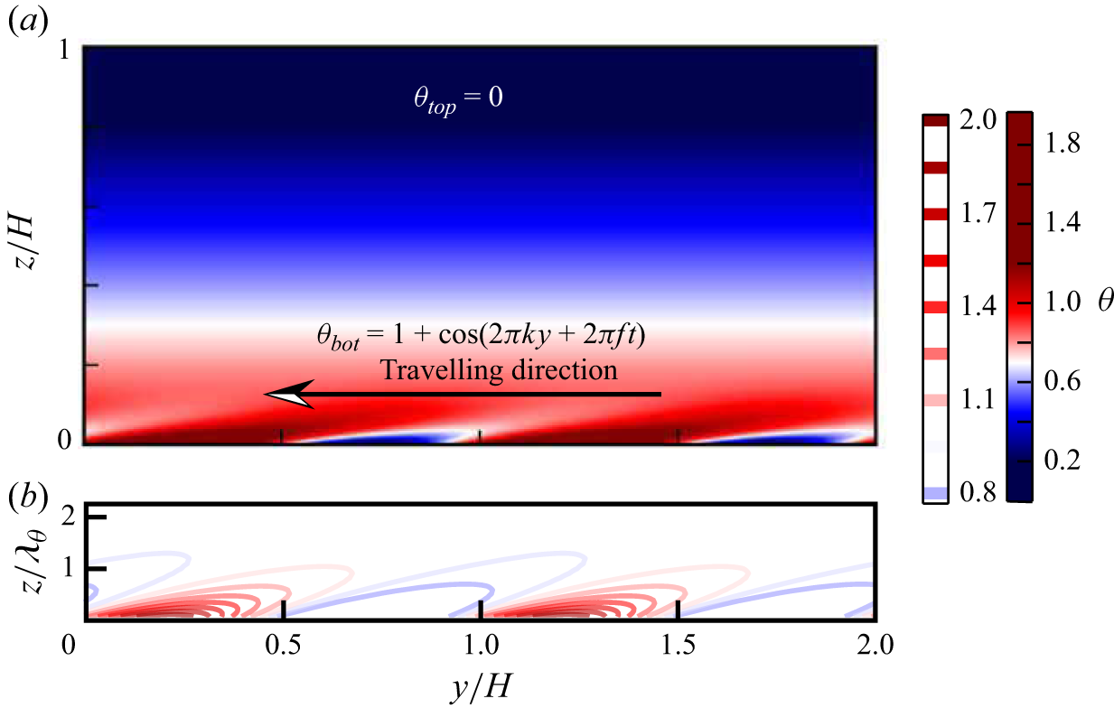
(a) Schematic of a two-dimensional convection cell with hybrid spatiotemporal modulation at the lower boundary and isothermal upper boundary. The aspect ratio is
 $\varGamma = W/H = 2$
. (b) Temperature isotherms near the thermal boundary layer.

2. Numerical method
We conduct direct numerical simulations of two-dimensional RB convection with hybrid spatiotemporal thermal modulation at the bottom boundary (see figure 1). The dimensionless governing equations under the Boussinesq approximation are
 \begin{align}&\qquad\qquad\qquad\qquad \boldsymbol{\nabla }\boldsymbol{\cdot }\boldsymbol{u} = 0, \end{align}
 \begin{align}& \frac {\partial \boldsymbol{u}}{\partial t} + (\boldsymbol{u} \boldsymbol{\cdot }\boldsymbol{\nabla }) \boldsymbol{u} = -\boldsymbol{\nabla }p + \left (\frac {\textit{Ra}}{\textit{Pr}}\right )^{-1/2} {\nabla} ^2 \boldsymbol{u} + \theta \boldsymbol{e}_z, \end{align}
 \begin{align}&\qquad\quad \frac {\partial \theta }{\partial t} + (\boldsymbol{u} \boldsymbol{\cdot }\boldsymbol{\nabla }) \theta = (Ra \, Pr)^{-1/2} {\nabla} ^2 \theta , \end{align}
where
 $t$
is the time scaled by the free-fall time
 $ \sqrt {H/(\alpha g \varDelta )}$
,
 $\boldsymbol{u}$
is the fluid velocity scaled by the free-fall velocity
 $ \sqrt {\alpha g \Delta H}$
,
 $\theta$
is the temperature scaled by the mean temperature difference
 $\varDelta$
between the two plates and
 $\boldsymbol{e}_z$
is the vertical unit vector. All length scales are normalised by the cell height
 $H$
. Periodic boundary conditions are imposed laterally for both the velocity and temperature fields. The top and bottom plates are impermeable and no-slip. The initial temperature field is assumed to be a linear profile. For the thermal boundary conditions, the top plate is maintained at a constant temperature (
 $\theta =0$
). The bottom plate is subjected to a hybrid spatiotemporal temperature distribution – namely, a thermal wave travelling at speed
 $c$
– which is expressed as
 \begin{equation} \theta (z=0, y, t) = 1 + \cos (2\pi f t + 2\pi k y)= 1+\cos (2\pi k(ct+y)). \end{equation}
The governing equations are solved using an in-house finite-difference solver, which has been extensively validated in previous studies (Verzicco & Orlandi Reference Verzicco and Orlandi1996; van der Poel et al. Reference van der Poel, Ostilla-Mónico, Donners and Verzicco2015; Ostilla-Monico et al. Reference Ostilla-Monico, Yang, van der Poel, Lohse and Verzicco2015), and with the code being applied to the case of temporal temperature modulation (Yang et al. Reference Yang, Chong, Wang, Verzicco, Shishkina and Lohse2020) and spatial temperature modulation (Zhao et al. Reference Zhao, Zhang, Wang, Wu, Chong and Zhou2022b
). All simulations are conducted at a fixed Prandtl number of
 $Pr = 4.3$
(corresponding to water at
 $40\,^{\circ}{\rm C}$
) and Rayleigh number of
 $Ra = 10^8$
, while systematically varying the modulation parameters over broad ranges: the modulation wavenumber
 $k$
from 4 to 80 and the modulation frequency
 $f$
from 0.001 to 6. To ensure adequate resolution, the grid is refined with wavenumber, ranging from
 $513 \times 257$
for
 $k = 4$
to
 $2561 \times 257$
for
 $k = 80$
, maintaining at least 15 points per modulation wavelength and within the thermal boundary layer (for details, see supplementary material, table S1, available at https://dx.doi.org/10.1017/jfm.2025.10651). Temporal resolution is set to a minimum of 15 steps per modulation cycle. Statistical convergence is rigorously ensured by conducting simulations over sufficiently long durations. The baseline cases are integrated for more than 600 free-fall time units, while simulations with particularly low frequencies (e.g.
 $f = 0.001$
) are extended up to 10 000 free-fall time units to capture at least 10 full modulation cycles. This strategy ensures reliable statistical sampling across the entire parameter space.
3. Results
We begin by examining the heat transport properties characterised by the Nusselt number
 $Nu$
, which is defined as
 \begin{equation} Nu = \sqrt {\textit{Ra}\,\textit{Pr}} \langle w\theta \rangle _{y,t} - \left \langle \frac {\partial \theta }{\partial z} \right \rangle _{y,t}, \end{equation}
where
 $w$
denotes the vertical component of the velocity field and
 $\langle \boldsymbol{\cdot }\rangle _{y,t}$
represents averaging over both time and horizontal line. In our analysis, we evaluate
 $Nu$
at the top and bottom plates. The computed values of
 $Nu_{\textit{top}}$
and
 $Nu_{\textit{bot}}$
differ by less than 1 %, confirming the accuracy of our numerical simulations.
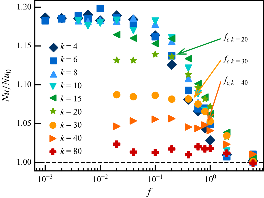
Figure 2 shows the normalised Nusselt number,
 $Nu/Nu_0$
, plotted as a function of modulation frequency
 $f$
for a range of wavenumbers
 $k$
. At low frequencies, which correspond to the spatially modulated scenarios,
 $Nu/Nu_0$
exhibits a plateau. This plateau level decreases monotonically with increasing
 $k$
. Beyond a
 $k$
-dependent critical frequency (e.g.
 $f_{{c},k=20} \approx 0.2$
,
 $f_{{c},k=30} \approx 0.5$
and
 $f_{{c},k=40} \approx 0.9$
), the normalised Nusselt number begins to decline, where the critical frequency increases with wavenumber. At sufficiently high frequencies (e.g.
 $f = 6$
for all cases),
 $Nu/Nu_0$
asymptotically approaches the baseline value corresponding to the unmodulated RB convection.
Normalised Nusselt number
 $Nu/Nu_0$
as a function of frequency
 $f$
for different wavenumbers
 $k$
, obtained at
 $Ra = 10^8$
and
 $Pr = 4.3$
. Here,
 $Nu_0$
denotes the Nusselt number for unmodulated RB convection. The horizontal dashed line indicates no significant heat transfer enhancement.

To interpret the observed trends in heat transfer efficiency, we examine the flow structures, particularly near the thermal boundary layer, which is intimately related to the heat transport efficiency. Figure 3 shows instantaneous temperature fields at
 $k = 6$
for varying modulation frequencies
 $f$
. At low
 $f$
shown in figure 3(a), thermal plume emission is triggered by the modulated plate, where the plumes penetrate deeply into the bulk and form a large-scale roll (see supplementary movie S1). As
 $f$
increases, which corresponds to an increase in the thermal wave speed
 $c$
, rapid shifts desynchronise plume emission from the hot region shown in figure 3(b). To illustrate this effect, we denote schematically the phase difference
 $\Delta \beta$
in the figure by tracking the centres of the modulated hot region and the plume, which reveals a loss of coherence between them (see supplementary movie S2). This decoupling suppresses the effective route of plume formation, diminishing heat transfer efficiency. At sufficiently high frequencies, as the thermal wave speed
 $c$
further increases (see figure 3
c), thermal perturbations become confined within the thermal boundary layer, and plume emission is hardly influenced by the modulation (see supplementary movie S3). Consequently, the heat transfer efficiency approaches that of the unmodulated RB convection.
Typical snapshots of instantaneous temperature fields (colour) and contours (lines) near the bottom boundary. (a–c) Results at fixed wavenumber
 $k=6$
for different frequencies: (a)
 $f=0.02$
, (b)
 $f=0.8$
and (c)
 $f=6$
. The arrows indicate the travelling direction of the thermal wave, and
 $c^*$
is the critical speed, which is discussed later. Here
 $\Delta \beta$
denotes the phase difference between the centre of the modulated heating region and the hot plume. (d) The unmodulated RB convection case for comparison. (e–g) Results for varying wavenumbers, (e)
 $k=6$
, (f)
 $k=20$
and (g)
 $k=80$
, each displaying the three frequencies
 $f=0.02$
,
 $0.8$
and
 $6$
. (h) Results for three wavenumbers
 $k=6$
,
 $20$
and
 $80$
at a fixed frequency
 $f=0.02$
. The averaged spatial correlation is calculated as
 $\sigma = \langle \mathbf{\theta }(z,t) \boldsymbol{\cdot }\mathbf{\theta }(z_0,t) / \mathbf{\theta }(z_0,t)^2 \rangle _{y,t}$
, where
 $\mathbf{\theta }(z_0,t)$
denotes the temperature field along the bottom boundary and
 $\langle \boldsymbol{\cdot }\rangle _{y,t}$
represents
 $y$
-direction and temporal averaging.

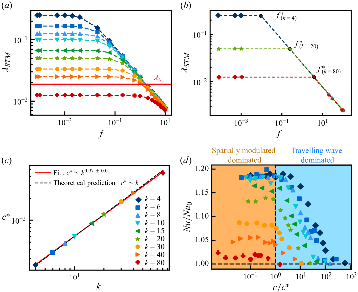
(a) Spatiotemporal penetration depth
 $\lambda _{\textit{STM}}$
versus modulation frequency
 $f$
for various wavenumbers
 $k$
. The red line represents the thermal boundary-layer thickness, estimated as
 $\lambda _{\theta } = (2Nu_0)^{-1}$
. (b) For each
 $k$
, we obtain
 $f^*$
by calculating the intersection of two fitted lines: one from the three leftmost points in the plateau region and the other from the three rightmost points in the decay region. (c) Critical speed
 $c^*$
, defined as
 $f^*$
divided by its corresponding
 $k$
, plotted as a function of
 $k$
. The theoretical prediction and the fitted scaling are denoted by the black dashed line and the red line, respectively. (d) Heat transfer efficiency
 $Nu/Nu_0$
as a function of normalised speed
 $c/c^*$
.

To further illustrate the decoupling between plume emission and heated regions induced by rapid travelling-wave shifts, we present time-averaged correlation profiles
 $\sigma (z)$
for various modulation frequencies and wavenumbers (see figure 3
e–g). In figure 3(e), for low wavenumber
 $k = 6$
, the correlation remains high across the vertical extent at low frequency
 $f = 0.02$
, indicating strong coherence of the thermal plumes. As the frequency increases, the correlation decays more rapidly with height, reflecting a loss of coherence due to the ‘smoothing’ effect of the fast-moving thermal wave. At higher wavenumbers, the correlation remains low across all frequencies in figure 3(g). Figure 3(h) presents the correlation coefficients for a fixed frequency
 $f=0.02$
across different modulation wavenumbers. The results indicate that the correlation coefficients decrease with increasing wavenumber, demonstrating that larger modulation wavenumbers suppress coherence of thermal plumes. These findings indicate that coherent plume structures are increasingly difficult to sustain under rapid and finely modulated boundary conditions.
What critical condition marks the onset of the ‘smoothing’ effect? What determines the diminishing influence of spatiotemporal modulation? To understand this issue, we derive the expression for the penetration depth, denoted as
 $\lambda _{\textit{STM}}$
, where STM denotes spatial–temporal modulation, based on the concept proposed in Yang et al. (Reference Yang, Chong, Wang, Verzicco, Shishkina and Lohse2020) and Zhao et al. (Reference Zhao, Zhang, Wang, Wu, Chong and Zhou2022b
). Specifically, we consider the diffusion equation in an infinite slab and solve it under spatiotemporal temperature modulation imposed on the bottom plate. The resulting expression is given by (see Appendix A)
 \begin{equation} \lambda _{\textit{STM}} = \left [\frac {k^2 + \sqrt {k^4 + \textit{Ra}\,\textit{Pr}\,(f/2\pi )^2}}{2}\right ]^{-1/2}. \end{equation}
Figure 4(a) shows
 $\lambda _{\textit{STM}}$
as a function of frequency
 $f$
for various wavenumbers
 $k$
. At low frequencies,
 $\lambda _{\textit{STM}}$
exhibits a plateau, whose level decreases monotonically with increasing
 $k$
. Above a
 $k$
-dependent threshold frequency, the plateau of
 $\lambda _{\textit{STM}}$
cannot be maintained, leading to a subsequent decline. As we set
 $f=0$
, it follows the scaling
 $\lambda _{\textit{STM}} = k^{-1}$
, consistent with previous results for purely spatial modulation (Zhao et al. Reference Zhao, Zhang, Wang, Wu, Chong and Zhou2022b
). This suggests that, in the low-frequency limit, the modulation depth is set by the spatial structure of the imposed boundary. However, in the high-frequency regime,
 $\lambda _{\textit{STM}}$
decreases with
 $f$
as
 $\lambda _{\textit{STM}} = [\sqrt {\textit{RaPr}}f/(4\pi )]^{-0.5}$
obtained by setting
 $k=0$
, consistent with previous results for purely temporal modulation (Yang et al. Reference Yang, Chong, Wang, Verzicco, Shishkina and Lohse2020). This indicates that the modulation depth is limited by both spatial modulation and temporal modulation.
To capture the transition between the spatially dominated regime at low
 $f$
and the travelling-wave-dominated regime at high
 $f$
, we define the critical frequency
 $f^*$
as the intersection of the tangents to the low-frequency plateau and the high-frequency decay branches in the
 $\lambda _{\textit{STM}}$
versus
 $f$
curve (see figure 4
b). Then, we obtain
 $c^*$
by dividing
 $f^*$
by its corresponding wavenumber as shown in figure 4(c). From this perspective, we obtain
 $[\sqrt{\boldsymbol{RaPr}}f^*/(4\pi )]^{-0.5} = k^{-1}$
, which leads to
 $f^*= 4\pi k^2/\sqrt {\textit{RaPr}}$
. Further, we get
 $c^*= f^*/k= 4\pi k/\sqrt {\textit{RaPr}}$
, the relation showing a good collapse as depicted in figure 4(c). The right-hand side is defined as the pseudo-speed of thermal diffusion,
 $c_{\textit{diff}} = 4\pi k/\sqrt {\textit{RaPr}}$
, a scale-dependent measure of thermal damping, and the left-hand side represents the critical speed of a travelling wave. When
 $c/c_{\textit{diff}} \gt 1$
, the flow transitions from spatially dominated to travelling-wave-dominated behaviour.
To confirm this proposed physical picture of the transition between distinct regimes, we replot
 $Nu/Nu_0$
as a function of
 $c/c^*$
for various values of
 $k$
in figure 4(d). The figure shows that the normalised
 $Nu$
begins to decrease to 1 when
 $c \gt c^*$
. Specifically, when spatiotemporal modulation is introduced, the boundary hotspot begins to move laterally at a wave speed. If this wave speed exceeds
 $c^*$
, the boundary thermal signal is displaced before it can fully develop, preventing coherent plume emission. This results in a spatial mismatch between the hotspot and the thermal plume, weakening convective transport.
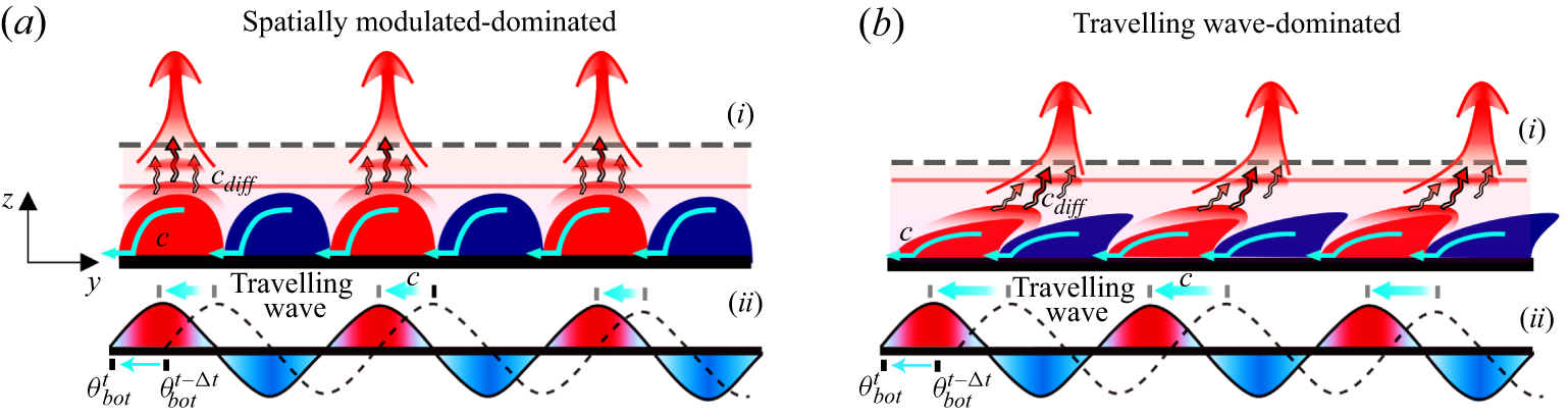
Schematic illustration of plume emission near the bottom plate in (a) the spatially modulated regime and (b) the travelling-wave-dominated regime. Panel (i) shows the flow structure, where red and blue regions indicate thermal diffusion from boundary heating. The grey dashed line marks the effective depth of spatiotemporal modulation, and the red solid line represents the thermal boundary layer
 $\lambda _\theta$
. Panel (ii) presents the bottom temperature profile: the solid line indicates the current state
 $\theta _{\textit{bot}}^t$
and the dashed line shows the earlier state
 $\theta _{\textit{bot}}^{t-\Delta t}$
.

4. Conclusion
In conclusion, we have examined heat transfer in RB convection subjected to hybrid spatiotemporal thermal modulation at the bottom boundary, using direct numerical simulations across a broad range of modulation frequencies and spatial wavenumbers. Our results reveal distinct regimes. At low modulation frequencies, spatial modulation dominates, organising thermal plumes and enhancing global heat transport. At high frequencies, the rapid propagation of the temperature wave exerts a ‘smoothing’ effect on the plumes, thereby reducing convective efficiency.
We show that the ‘smoothing’ effect induces a transition between these regimes, governed by the competition between the wave speed (
 $c =f/k$
) and the pseudo-speed of thermal diffusion,
 $c_{\textit{diff}} = 4\pi k/\sqrt {\textit{RaPr}}$
, a scale-dependent measure of thermal damping. Specifically, when
 $c \lt c_{\textit{diff}}$
, spatial modulation dominates. In this regime, the slow boundary thermal wave allows high-temperature regions enough time to evolve, keeping the thermal hotspots well aligned with the diffusive zone and enabling coherent thermal plumes to emerge and form stable, continuous channels for thermal transport (see figure 5
a).
In contrast, when
 $c \gt c_{\textit{diff}}$
, the fast-moving travelling wave disrupts the spatial coherence of the plumes, suppressing convective transport (see figure 5
b). These findings provide mechanistic insights into how hybrid spatiotemporal modulation governs thermal transport in convective systems, highlighting the critical role of the wave speed and thermal diffusion competition. Our work offers predictive guidelines for optimising heat transfer through targeted control of modulation parameters, with potential applications in engineered thermal systems and in interpreting heat exchange in geophysical problems where spatiotemporal modulation is present. In particular, the ratio
 $c/c_{\textit{diff}}$
may serve as a key control parameter for understanding surface–atmosphere heat transfer under naturally varying spatiotemporal thermal modulation.
Supplementary material and movies
Supplementary material and movies are available at https://doi.org/10.1017/jfm.2025.10651.
Funding
This work is supported by NSFC Excellence Research Group Program for ‘Multiscale Problems in Nonlinear Mechanics’ (no. 12588201). It was also supported by the Natural Science Foundation of China under grant nos. 12372219, 52450304, 12432011, 12422208, 12421002 and 12372220 and by the China Postdoctoral Science Foundation under grant no. 2024M761631.
Declaration of interests
The authors report no conflict of interest.
Appendix A. Solution for pure diffusion state under travelling thermal wave
For pure diffusion under a travelling thermal wave, the governing equations and the boundary conditions read
 \begin{align}&\qquad\qquad\quad \partial _t T - \kappa {\nabla} ^2 T = 0, \end{align}
 \begin{align}& T = \begin{cases} T_{\textit{hot}} + A \cos (\omega t + k x), \text{at $z = 0$,}\\ T_{\textit{cold}}, \text{at $z = H$.} \end{cases} \end{align}
We define
 $T = T_{{cold}}+(H-z)\varDelta /H + T_{\textit{mod}}$
. Then (A1) becomes
 \begin{align}&\qquad\quad \partial _t T_{\textit{mod}} - \kappa {\nabla} ^2 T_{\textit{mod}} = 0, \end{align}
 \begin{align}& T_{\textit{mod}} = \begin{cases} A \cos (\omega t + k x), \text{at $z = 0$,}\\ 0, \text{at $z = H$.} \end{cases} \end{align}
Applying the Fourier transform on (A3) in the horizontal direction and time, one obtains
 \begin{align}&\qquad\qquad\qquad\qquad \partial _z \partial _z \hat {T}_{\textit{mod}} - ({\rm i}\varOmega /\kappa + K^2) \hat {T}_{\textit{mod}} = 0,\nonumber\\[-10pt] \end{align}
 \begin{align}& \hat {T}_{\textit{mod}} = \begin{cases} 2\pi^{2} A \delta (\omega - \varOmega )\delta (k-K) + 2\pi^{2} A \delta (\omega + \varOmega )\delta (k+K),\quad \text{at $z = 0$,}\\ 0,\quad \text{at $z = H$.} \end{cases} \end{align}
For the characteristic equation, we obtain two racines
 $\pm \sqrt {({\rm i}\varOmega /\kappa + K^2)}$
. We define that the real part of (A5) and (A6), one can find an analytical solution:
 \begin{equation} \hat {T}_{\textit{mod}} = C_1 {\rm e}^{\sqrt {{\rm i}\varOmega /\kappa + K^2} z} + C_2 {\rm e}^{-\sqrt {{\rm i}\varOmega /\kappa + K^2} z} , \end{equation}
where the coefficients
 $C_1$
and
 $C_2$
are obtained from the boundary conditions, and taking the inverse Fourier transform. Defining
 $\sqrt {{\rm i}\omega /\kappa + k^2} = \zeta + {\rm i} \xi$
and
 $\sqrt {-{\rm i}\omega /\kappa + k^2} = \zeta - {\rm i} \xi$
, one can obtain one analytical solution for (A3) and (A4):
 \begin{equation} {T}_{\textit{mod}} = \frac { A \sinh [-(\zeta + {\rm i}\xi )(z-1)]}{2 \sinh (\zeta + {\rm i}\xi )} {\rm e}^{{\rm i}(\omega t + k x)} + \frac { A \sinh [-(\zeta -{\rm i}\xi )(z-1)]}{2 \sinh (\zeta - {\rm i}\xi )} {\rm e}^{-{\rm i}(\omega t + k x)}. \end{equation}
The decay rate in the vertical direction can be described by
 $\zeta = [(k^2+\sqrt {k^4+\textit{RaPr}\omega ^2})/2]^{1/2}$
, obtained from
 ${\rm e}^{-\zeta z}$
in dimensionless form.
Considering the current form of our thermal boundary conditions at the bottom plate, and choosing the depth at which the modulation decays to
 ${\rm e}^{-2\pi }$
of the original value following the work by Zhao et al. (Reference Zhao, Zhang, Wang, Wu, Chong and Zhou2022b
), using
 ${\rm e}^{-2\pi \zeta ^{\prime } z}$
with
 $\zeta ^{\prime }=\zeta /2\pi$
. Finally, we get the spatiotemporal modulation depth, expressed as
 \begin{equation} \lambda _{\textit{STM}}= \left(\zeta ^{\prime }\right)^{-1}= \left[\left( k^2+\sqrt {k^4+\textit{RaPr}(f/2\pi )^2}\right)/2\right]^{-1/2}. \end{equation}