1. Introduction
The transverse jet or jet in crossflow (JICF) is a canonical flowfield which has many applications for mixing and reaction enhancement in energy and propulsion systems (Margason Reference Margason1993; Karagozian Reference Karagozian2010, Reference Karagozian2014). The present study focuses on round gaseous jets (mixtures of helium and nitrogen) injected perpendicularly into a crossflow of air. Some of the characteristic parameters of this flowfield include the jet-to-crossflow velocity ratio,
 $R\equiv U_{j}/U_{\infty }$
, the jet-to-crossflow density ratio,
 $S\equiv {\it\rho}_{j}/{\it\rho}_{\infty }$
, the jet-to-crossflow momentum flux ratio,
 $J\equiv SR^{2}$
, and the jet Reynolds number,
 $\mathit{Re}_{j}\equiv U_{j}D/{\it\nu}_{j}$
, based on the jet exit diameter
 $D$
, the bulk jet velocity
 $U_{j}$
and kinematic viscosity of the jet fluid,
 ${\it\nu}_{j}$
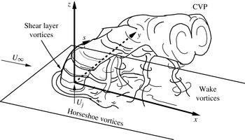
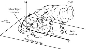
. The interaction of the jet and crossflow creates a complex set of vortex systems, as shown for the transverse jet with flush injection in figure 1.
Schematic of the transverse jet, introduced flush with respect to the injection wall, including relevant vortical structures such as the jet upstream shear layer vortices and CVP. Orientation of coordinate axes
 $x,y,z$
and shear layer trajectory
 $s$
are shown. Adapted from Fric & Roshko (Reference Fric and Roshko1994).
The transverse jet cross-section has long been observed to be dominated by a counter-rotating vortex pair (CVP) structure (Kamotani & Greber Reference Kamotani and Greber1972), which is thought to be generated in the near-field region of the jet, within a few diameters of injection, and associated with the evolution of vorticity in the upstream shear layer (Kelso, Lim & Perry Reference Kelso, Lim and Perry1996; Cortelezzi & Karagozian Reference Cortelezzi and Karagozian2001) as well as the pressure differences between the upstream and downstream regions of the jet (Muppidi & Mahesh Reference Muppidi and Mahesh2007). Experiments by Kelso et al. (Reference Kelso, Lim and Perry1996) in both water and air suggest that periodic shear layer vorticity rollup occurs for the jet in crossflow similarly to that which occurs in the free jet, yet the presence of crossflow leads to a tilting and folding of the cylindrical vortex sheet. This distortion of the vortex sheet has long been thought (Moussa, Trischka & Eskinazi Reference Moussa, Trischka and Eskinazi1977; Andreopoulos Reference Andreopoulos1985; Kelso et al.
Reference Kelso, Lim and Perry1996) to contribute to the circulation of the CVP; these ideas have been confirmed in the transient vortex element simulations of Cortelezzi & Karagozian (Reference Cortelezzi and Karagozian2001), for example. In addition to the CVP, other prevalent structures include horseshoe vortices, which wrap around the jet column and have been shown to become unsteady at velocity ratios
 $R$
of 2 and 4, and jet Reynolds numbers above approximately 2500 (Kelso & Smits Reference Kelso and Smits1995). Transient wake vortices are also present in the flush-injected JICF, and have been determined to contain wall boundary layer fluid which is drawn into the deflected jet (Fric & Roshko Reference Fric and Roshko1994).
Transverse jet shear layer vortices themselves have been thought to arise from a Kelvin–Helmholtz instability in the upstream shear layer between the jet and crossflow near the jet exit (Kelso et al.
Reference Kelso, Lim and Perry1996; Yuan & Street Reference Yuan and Street1998). Yet more recent experimental explorations (Megerian et al.
Reference Megerian, Davitian, Alves and Karagozian2007; Davitian et al.
Reference Davitian, Getsinger, Hendrickson and Karagozian2010; Getsinger, Hendrickson & Karagozian Reference Getsinger, Hendrickson and Karagozian2012) of transverse jet upstream shear layer instabilities have shown that the nature of this flowfield is much more complex. For jets injected from a smoothly contracting nozzle which is flush with respect to the tunnel wall, with fixed jet Reynolds numbers in the range
 $1800\leqslant \mathit{Re}_{j}\leqslant 3000$
, as jet-to-crossflow momentum flux ratio is lowered below approximately
 $J\approx 10$
, or as jet-to-crossflow density ratio is lowered below
 $S\approx 0.40$
, the upstream shear layer undergoes a transition from being convectively unstable to being absolutely unstable (Huerre & Monkewitz Reference Huerre and Monkewitz1990), in the case of the latter, creating strong, pure-tone oscillations that are relatively insensitive to external excitation. The extensive evidence for this shear layer transition from convective to absolute instability includes a reduction in the energy transfer from fundamental to subharmonic frequencies along the jet shear layer, flow transition to a global mode via a Hopf bifurcation, and ‘lock-in’ of the shear layer to an applied excitation frequency close to the fundamental or further from the fundamental but at a high amplitude of excitation (Davitian et al.
Reference Davitian, Getsinger, Hendrickson and Karagozian2010; Getsinger et al.
Reference Getsinger, Hendrickson and Karagozian2012). This evidence has largely been quantified via hot-wire anemometry. Recent direct numerical simulations (DNS) of the equidensity JICF (Mahesh & Iyer Reference Mahesh and Iyer2013) with flush nozzle conditions identical to those in the experiments of Megerian et al. (Reference Megerian, Davitian, Alves and Karagozian2007) for absolutely unstable and convectively unstable conditions (at velocity ratios
 $R=2$
and 4, respectively) show excellent quantitative agreement in velocity spectral characteristics, and thus are consistent with the experimentally observed transition.
In experiments, a similar transition in shear layer stability characteristics is observed for an elevated contracting nozzle which injects the jet fluid into crossflow above the injection wall boundary layer (Megerian et al.
Reference Megerian, Davitian, Alves and Karagozian2007). Because the interior geometry of the flush and elevated nozzles is matched in that study, each has essentially the same near-top-hat velocity profile at the jet exit in the absence of crossflow. Yet for the elevated nozzle, this transition from convective to absolute shear layer instability occurs at a much lower momentum flux ratio, approximately
 $J\approx 0.93$
based on mean jet velocity, due to vertical coflow effects adjacent to the upstream side of the nozzle as crossflow velocity
 $U_{\infty }$
is increased. To our knowledge, there have been no detailed experimental or computational studies of the upstream shear layer instability transition for a transverse jet produced by a straight pipe with a fully developed exit profile in the absence of crossflow. Pipe-generated transverse jet experiments in water by Camussi, Guj & Stella (Reference Camussi, Guj and Stella2002), however, do suggest that the onset of the shear layer instability is driven by ‘a destabilization mechanism different from the Kelvin–Helmholtz instability’, with a very strong oscillation or ‘waving’ in the flow for
 $R<3$
.
Mixing quantification associated with the transverse jet cross-section as well as the longitudinal centreplane (
 $y=0$
plane) of the jet can be quite dependent on specific jet structural characteristics, in that a centreplane slice of the jet may or may not capture the predominant distribution of jet fluid in the flowfield. While experiments over the years have shown the transverse jet cross-section to contain a relatively symmetric CVP, as indicated in figure 1 (Lim, New & Luo Reference Lim, New and Luo2001; Beresh et al.
Reference Beresh, Henfling, Erven and Spillers2006; New, Lim & Luo Reference New, Lim and Luo2006), even the earliest experiments on the JICF show slightly asymmetric cross-sectional characteristics for
 $J=15.3$
and 59.6 (Kamotani & Greber Reference Kamotani and Greber1972). For relatively high velocity ratios (
 $R=10$
and
 $R=20$
) and jet Reynolds numbers (16 000 and 33 000), Smith & Mungal (Reference Smith and Mungal1998) show unequal concentrations of jet fluid about the centreplane of the jet, both in instantaneous snapshots and in the ensemble averaged field, with increasing asymmetry as either jet-to-crossflow velocity ratio or distance downstream is increased. Experiments by Kuzo (Reference Kuzo1995) explore the asymmetry phenomenon using particle image velocimetry (PIV) measurements of the jet cross-section, and show that asymmetry is most apparent below a cutoff jet Reynolds number which increases with increasing jet-to-crossflow velocity ratio. Kuzo’s velocity measurements also show tertiary vortices below the familiar CVP which skew the orientation of the entire jet cross-section. Shan & Dimotakis (Reference Shan and Dimotakis2006) find a similar trend in liquid transverse jet experiments at
 $R=10$
, in which asymmetry of the jet cross-section and appearance of tertiary vortices occurs as jet Reynolds number is decreased from 2000 to 1000.
It should be noted that all the experiments which show significant degrees of asymmetry for the JICF use jet fluid injection that is flush with respect to the tunnel wall, and most involve contracting nozzles. The forced and unforced transverse jet experiments of Narayanan, Barooah & Cohen (Reference Narayanan, Barooah and Cohen2003) at
 $R=6$
and
 $\mathit{Re}_{j}=5000$
for a flush pipe-injected jet with a fully developed velocity profile at the exit plane do show slight asymmetries in the mean in the CVP in the absence of external forcing, especially further downstream. DNS designed to replicate these flow conditions by Muldoon & Acharya (Reference Muldoon and Acharya2010) indeed show an asymmetry in the jet cross-section (
 $yz$
-plane), which is said to be associated with symmetry-breaking initial conditions. The authors note that, under the conditions examined, the flow is very susceptible to asymmetries and that such ‘asymmetric states’ could appear in an experiment in which asymmetries in initial or boundary conditions could be present.
The above studies suggest that, while there is a logical connection between the transverse jet shear layer vorticity and the formation of the CVP (Kelso et al. Reference Kelso, Lim and Perry1996), there are clearly conditions for which the flow structure can be asymmetric about the centreplane, even in the temporally averaged flowfield. The goal of the present experimental studies is to examine the relationships between transverse jet structural characteristics and shear layer instabilities for a range of operating conditions. It is anticipated that this focus will enable a more robust understanding of transverse jet behaviour and structural characteristics, with eventual implications for transverse jet mixing and optimized control.
2. Experimental facility and methods
2.1. Transverse jet wind tunnel
The present transverse jet studies employ a low-speed blower-type wind tunnel used in prior experiments (Megerian et al.
Reference Megerian, Davitian, Alves and Karagozian2007; Davitian et al.
Reference Davitian, Getsinger, Hendrickson and Karagozian2010; Getsinger et al.
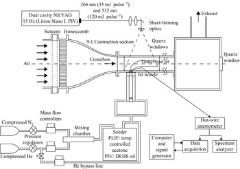
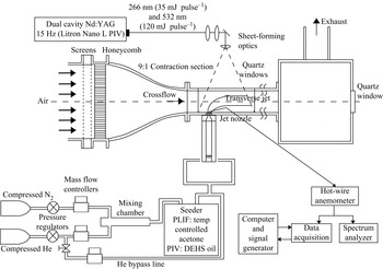
Reference Getsinger, Hendrickson and Karagozian2012), shown in figure 2. Before entering the 9:1 area ratio contraction section, the air from a centrifugal blower was conditioned using honeycomb and screens of decreasing mesh size in order to break down turbulent structures to smaller (dissipative) scales. The maximum attainable free-stream crossflow velocity,
 $U_{\infty }$
, was
 $7.0\ \text{m}\ \text{s}^{-1}$
with a maximum turbulence intensity of less than 1.5 % in the free stream. The test section was 30 cm long and
 $12\ \text{cm}\times 12\ \text{cm}$
in cross-section, fitted flush with the exit of the tunnel contraction. A quartz window was mounted to the top surface of the test section for laser sheet introduction, and Plexiglas optical access windows were mounted to the sides. All other interior surfaces were spray painted matte black to reduce reflection. One additional tunnel section of equal dimensions (without optical access) was mounted flush with the end of the primary test section, followed by a
 $30\ \text{cm}\times 30\ \text{cm}\times 30\ \text{cm}$
chamber with an exhaust duct attached to the top. This chamber was fitted with a
 $90\ \text{mm}\times 90\ \text{mm}$
quartz window that allowed optical access from downstream looking upstream in the negative
 $x$
direction for jet cross-sectional (
 $yz$
-plane) imaging.
Variable-density transverse jet wind tunnel, with associated data acquisition and optical diagnostic apparatus. One additional tunnel section, of identical dimensions, was situated downstream of the test section shown.
For the present experiments, the jet fluid consisted of mixtures of gaseous nitrogen and helium supplied by two separate gas cylinders, allowing control of the jet-to-crossflow density ratio by variation in the relative flow rates of each gas. Each cylinder was regulated and delivered flow via separate mass flow controllers (Tylan FC-260 and Sierra Instruments C100L) into a passive mixing chamber. Depending on the optical measurement technique, the jet fluid exiting the passive mixing chamber was routed through one of two separate flow seeders: an acetone bubbler for planar laser-induced fluorescence (PLIF) measurements, or an aerosol generator for PIV. After flowing through one of these seeders, the mixture passed into a Plexiglas pipe via four symmetrically oriented inlet fittings before reaching the nozzle.
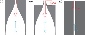
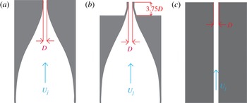
The gas exiting the pipe was then fed into the jet injector. Three alternative injectors were employed in the present study, each with a 4 mm exit diameter, shown schematically in figure 3. The two nozzles have been studied in prior experiments (Megerian et al.
Reference Megerian, Davitian, Alves and Karagozian2007). They had similar fifth-order polynomial contraction contours that created thin jet boundary layers for an essentially top-hat-like jet exit velocity profile in the absence of crossflow. The only significant difference between the two nozzles was that one had an exit plane mounted flush with the test section floor, whereas the other had an exit plane that was elevated above the tunnel floor by approximately 3.75 diameters. Hence the elevated nozzle allowed injection of jet fluid outside of the crossflow boundary layer, which had a maximum value of
 ${\it\delta}_{99\,\%}/D\approx 2.3$
for the lowest crossflow velocity condition explored here,
 $U_{\infty }=1.01\ \text{m}\ \text{s}^{-1}$
.
Alternative jet injectors studied: (a) flush nozzle, (b) elevated nozzle, and (c) straight pipe.
A third injector in the present studies consisted of a straight pipe with the same inner diameter as each nozzle at the exit plane and with a length
 $L$
such that
 $L/D=155$
. The straight pipe was verified to have created a fully developed pipe flow velocity profile at the exit plane, to enable comparison of jet structural characteristics with those for injection from the contoured nozzles. The jet Reynolds number for all injectors was based on bulk jet velocity,
 $U_{j}$
, determined by the specified mass flow rate of the jet fluid, the jet fluid density,
 ${\it\rho}_{j}$
, and the mixture viscosity (including the effect of acetone if present). The jet Reynolds number was held constant at
 $\mathit{Re}_{j}=1900$
for the majority of the cases studied here, except when Reynolds number effects on jet structure were explored. The jet-to-crossflow density ratio
 $S$
was likewise fixed at
 $S=1.00$
for most of the results shown, except for those for which
 $J$
and
 $\mathit{Re}_{j}$
were fixed and
 $S$
was varied. Details on the methods for determining jet density and transport properties for these mixtures may be found in Getsinger (Reference Getsinger2012).
2.2. Flow measurements and planar imaging
Hot-wire anemometry was used (in the absence of acetone or other seeding) to examine the shear layer characteristics of jets at a series of matched values of
 $J$
and
 $\mathit{Re}_{j}$
for each of the three injector types, as has been done in prior studies (Megerian et al.
Reference Megerian, Davitian, Alves and Karagozian2007; Davitian et al.
Reference Davitian, Getsinger, Hendrickson and Karagozian2010; Getsinger et al.
Reference Getsinger, Hendrickson and Karagozian2012). A single-component, boundary-layer-type probe (Dantec 55P15) enabled quantification of the shear layer velocity spectra corresponding to fluctuations in the vertical velocity component
 $u_{z}$
. The hot-wire probe could be traversed along the transverse jet upstream shear layer in the
 $y=0$
plane with an accuracy of
 $1\ {\rm\mu}\text{m}$
. Determination of these shear layer trajectories (coordinate
 $s$
in figure 1) required performing traversals at a series of elevations in
 $z$
above the jet exit, as described in Megerian et al. (Reference Megerian, Davitian, Alves and Karagozian2007). Loci of the local velocity profile inflection point and maxima in fluctuation amplitude within the velocity profile provided data from which the shear layer trajectory
 $s$
was determined. The hot-wire probe was operated in conjunction with a Dantec constant-temperature anemometer and delivered to a dynamic signal analyser (HP 35665A). All shear layer spectra were ensemble averaged over 40 individual acquisitions.
Although hot-wire anemometry can provide insight into stability characteristics of the near-field transverse jet shear layer, the use of planar optical diagnostics enables non-intrusive exploration, and this has been a natural evolution of our studies. PLIF of acetone vapour seeded into the jet fluid was chosen as a primary means of determining the influence of the state of the upstream shear layer stability on the overall transverse jet structure, with the laser sheet enabling both centreplane (
 $xz$
-plane) and cross-sectional (
 $yz$
-plane) jet slices to enable jet concentration quantification and visualization. Non-intrusive velocity measurements were also performed here, in the near-field of the equidensity transverse jet, using stereoscopic PIV, selected to enable measurement of each of the in- and out-of-plane velocity components as well as accurate vorticity field measurements.
A schematic of the general set-up for planar imaging in the transverse jet is included in figure 2. The excitation source for both PLIF and PIV was a dual cavity
 $Q$
-switched Nd:YAG laser (Litron Nano L PIV), which was equipped with both second- and fourth-harmonic generation for simultaneous collinear output at 532 nm and 266 nm. Each laser cavity had an energy output of approximately
 $35\ \text{mJ pulse}^{-1}$
at 266 nm and
 $120\ \text{mJ pulse}^{-1}$
at 532 nm in an 8 ns full width at half maximum (FWHM) period. While the maximum laser repetition rate was 15 Hz, in general practice the laser was operated at no greater than 2 Hz, mainly to avoid ablation of the paint on the tunnel floor used to reduce reflection, but also to ensure statistical independence of the images. Timing of the laser pulses as well as image acquisition were achieved using a PC equipped with an external programmable timing unit (PTU) and DaVis 8.1 control software from LaVision.
The beam was formed into a thin, divergent sheet and directed into the test section by a combination of two spherical lenses, a turning mirror, and an
 $f=-10\ \text{mm}$
cylindrical lens, entering the test section through the upper quartz window. Rotation of the cylindrical lens by 90° allowed measurements to be made in either the
 $y=0$
jet centreplane or at constant-
 $x$
jet cross-sections in the
 $yz$
-plane. The wind tunnel was mounted to a traversing platform which could be precisely moved in the crossflow (
 $x$
) direction by a lead-screw/stepper motor device in order to make measurements at varying
 $yz$
-plane cross-sections without altering the optical set-up. The use of acetone as a molecular tracer in PLIF is an extensively utilized technique for concentration, temperature and pressure measurements in gaseous flows (Lozano, Yip & Hanson Reference Lozano, Yip and Hanson1992; Smith & Mungal Reference Smith and Mungal1998; Thurber et al.
Reference Thurber, Grisch, Kirby, Votsmeier and Hanson1998; Su & Mungal Reference Su and Mungal2004). For isothermal flows in which the excited fluid medium is optically thin, fluorescence intensity is proportional to both the laser fluence (assuming absorption saturation is not reached) and the acetone concentration (Lozano Reference Lozano1992; Lozano et al.
Reference Lozano, Yip and Hanson1992).
For our experiments involving only acetone PLIF, the laser beam was directed to a set of two 266 nm dichroic mirrors prior to reaching the sheet-forming optics, which separated the wavelengths and removed the majority of the 532 nm light. Approximately 10 % of the 266 nm beam energy was then deflected by a 3 mm thick UV grade fused silica window and directed to a pyroelectric joulemeter for pulse-to-pulse energy monitoring and recording to a PC via USB. The thickness of the laser sheet, as determined by traversing a razor blade through the sheet and measuring the
 $1/\text{e}^{2}$
thickness, ranged from approximately
 $400{-}900\ {\rm\mu}\text{m}$
in the camera field of view.
Fluorescence images were captured by a 14-bit CCD camera (LaVision Imager proX) with
 $1600\ \text{pixel}\times 1200\ \text{pixel}$
resolution, equipped with an external image intensifier (LaVision IRO) to boost the signal-to-noise ratio (SNR). All cross-sectional images were taken with a Nikon 200 mm lens at f/4.0. The equidensity (
 $S=1$
) and
 $S=0.55$
centreplane images were taken with a Nikon 50 mm lens at f/2.0 equipped with a Vivitar
 $+2$
dioptre close-up lens, and
 $S=0.35$
centreplane images were taken with a Sigma AF 90 mm at f/2.8. All lens configurations were equipped with a bandpass filter to isolate the fluorescence signal.
For centreplane imaging, the camera was located on one side of the tunnel test section, viewing the jet through a Plexiglas window. Centreplane image resolution ranged from 140 to
 $170\ {\rm\mu}\text{m}$
per pixel after
 $2\times 2$
hardware binning was administered to increase the SNR for density ratios
 $S=1$
and
 $S=0.55$
. When imaging cross-sectional slices of the jet in the
 $yz$
plane, the camera was moved to the rear of the wind tunnel, viewing the fluorescence through the quartz window on the end of the crossflow exhaust section. Cross-sectional data resolution ranged from 120 to
 $160\ {\rm\mu}\text{m}$
per pixel after
 $2\times 2$
binning. The image intensifier was triggered by the PC and PTU, and was gated at 200 ns, ensuring capture of the fluorescence and rejection of acetone phosphorescence, which occurs over a much larger timescale (approximately
 $200\ {\rm\mu}\text{s}$
) and which is strongly quenched by oxygen. With a temporal spacing between the two laser pulses set to 50 ns, the fluorescence signal captured by the camera was doubled from that of a single pulse with negligible motion blurring (
 $70\ \text{mJ pulse}^{-1}$
combined).
Acetone seeding was accomplished by bubbling the
 $\text{N}_{2}/\text{He}$
mixture comprising the jet fluid through a
 $17.8\ \text{cm tall}\times 19.1\ \text{cm}$
diameter chamber, filled with approximately 11.4 cm of liquid acetone prior to each measurement. Seeder chamber pressure was measured by a pressure transducer (Omega PX409-015G5V) and temperature by a Type T thermocouple, allowing the acetone concentration in the exiting jet fluid to be determined by consideration of the temperature dependence of acetone vapour pressure (Lozano Reference Lozano1992), under the assumption that the carrier gas flow became saturated with acetone vapour. The seeder temperature was maintained constant throughout data acquisition run times for a given jet flow condition by using a refrigerated recirculator to flow water through copper coils submerged in the liquid acetone, ensuring a constant seeding density. This seeder temperature was altered between flow conditions corresponding to different jet-to-crossflow density ratios
 $S$
for control of the acetone seeding level (ranging between 12 ° and 20 °C, corresponding to acetone concentrations ranging between approximately 11 % and 24 % by volume). The length of tubing between the exit of the seeder and the jet injector was sufficient for the jet fluid mixture to reach room temperature prior to entering the test section. The impact of the acetone vapour on mixture density and viscosity, estimated by the Reichenberg method (Poling, Prausnitz & O’Connell Reference Poling, Prausnitz and O’Connell2001), which takes into account the polarity of acetone, was included in the formulation of the required flow rates of each gas to meet desired values of
 $S$
and
 $J$
while maintaining the desired jet Reynolds number. The acetone vapour seeding into the jet fluid required that some helium needed to be mixed with the nitrogen and acetone to create gas mixtures with the desired density, even in the case where density ratio
 $S=1.00$
. Post-processing of the PLIF images included a set of standard corrections to account for bias errors and shot-to-shot fluctuations in order to convert pixel values into jet fluid concentration, as detailed in Getsinger (Reference Getsinger2012).
The stereoscopic PIV system utilized the same double-pulsed Nd:YAG laser and sheet-forming optics used for the acetone PLIF measurements. For PIV, the dichroic mirrors used to isolate the 266 nm wavelength as well as the beamsplitter/joulemeter were removed, allowing the 532 nm light to be the dominant excitation source. The thickness of the 532 nm laser sheet was measured to be approximately 1–1.5 mm within the imaging region in the jet
 $y=0$
centreplane. Seeding of the crossflow was achieved using a commercial fog machine (Pea Soup Rocket), with particles introduced into the fan of the crossflow blower. The jet fluid was seeded by diverting part of the injection line through a TSI particle generator containing di-ethyl-hexyl-sebacate (DEHS) oil.
The flowfield was imaged by two 14-bit cross-correlation CCD cameras (LaVision Imager proX,
 $1600\ \text{pixel}\times 1200\ \text{pixel}$
resolution), separated by a 60° angle (about the
 $z$
-axis) and oriented at a 90° light scattering angle. Each PIV camera was equipped with a Nikon 60 mm lens at f/8.0, a 532 nm narrowband filter, and a Scheimpflug lens mount. Further details on the calibration and extraction of the velocity field may be found in Getsinger (Reference Getsinger2012). The vector fields were computed using a multi-pass stereo correlation algorithm (LaVision DaVis 8.1.) with a final refinement step interrogation window size of
 $32\ \text{pixel}\times 32\ \text{pixel}$
. Each interrogation window had a Gaussian weighting function applied and was overlapped by 75 % to increase the number of vectors, yielding a
 $204\times 147$
grid with
 $162\ {\rm\mu}\text{m}$
grid spacing. The resulting ratio of the jet diameter to vector grid size
 ${\rm\Delta}x_{u}$
was therefore
 $D/{\rm\Delta}x_{u}\approx 26$
, while the ratio of diameter to size of the interrogation window
 ${\rm\Delta}x_{w}$
was
 $D/{\rm\Delta}x_{w}\approx 6.5$
. The time between laser pulses,
 ${\rm\Delta}t=25\ {\rm\mu}\text{s}$
, was considerably shorter than naturally occurring oscillations in the shear layer, which were of the order of 1 ms.
3. Results
3.1. Upstream shear layer stability and vorticity rollup
Stability characteristics of transverse jet shear layers quantified in the past via hot-wire measurements (Megerian et al.
Reference Megerian, Davitian, Alves and Karagozian2007; Davitian et al.
Reference Davitian, Getsinger, Hendrickson and Karagozian2010; Getsinger et al.
Reference Getsinger, Hendrickson and Karagozian2012) show significant alterations in the upstream shear layer spectral characteristics as velocity ratio
 $R$
or momentum flux ratio
 $J$
is reduced for a fixed set of jet Reynolds numbers. PIV in the present studies indicated a strong correspondence between shear layer stability conditions and shear layer vorticity rollup.
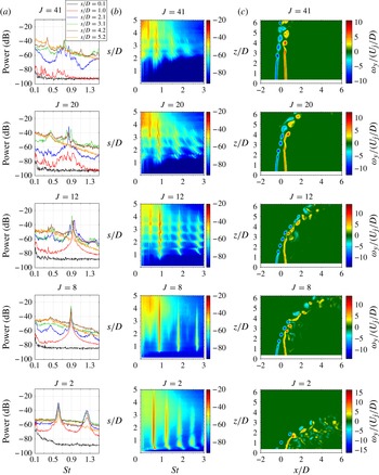
Figure 4(a), for example, shows the vertical velocity power spectra measured by the hot wire at several positions along the upstream shear layer (scaled distance
 $s/D$
) for the equidensity JICF created by the flush nozzle. Here
 $\mathit{Re}_{j}=1900$
was fixed, so that varying crossflow velocity
 $U_{\infty }$
produced a range of jet-to-crossflow momentum flux ratios, from
 $J=41$
to
 $J=2$
. The shear layer frequency content
 $f$
is scaled in terms of the Strouhal number,
 $St_{j}\equiv f\,D/U_{j}$
. As in prior studies, these power spectra demonstrated clear evidence of convectively unstable shear layers at high
 $J$
values, with relatively weak and broadband peaks, multiple modes created by tonal interaction with the hot wire (Getsinger et al.
Reference Getsinger, Hendrickson and Karagozian2012), and the generation of subharmonic instabilities. Such tonal interactions were not observed for the free jet,
 $J\rightarrow \infty$
(Megerian et al.
Reference Megerian, Davitian, Alves and Karagozian2007). When
 $J$
was reduced below around 10 (
 $R$
below approximately 3.1 for the equidensity case) by increasing the velocity of the crossflow and fixing that of the jet, the shear layer began to demonstrate typical absolutely unstable characteristics, with strong single-tone oscillation and higher harmonics, along with a weakening and eventual absence of subharmonics at lower
 $J$
. Figure 4(b) provides a more detailed representation of the power spectra on a finer spatial grid (
 ${\rm\Delta}s/D=0.1$
) via spectral magnitude contour plots, indicating the strength of the instabilities and corresponding Strouhal number for various locations along the shear layer. These contour plots enable distinctive characteristics of the transverse jet shear layer to be identified, contrasting more clearly the convective and absolute instability differences, as done in prior studies (Megerian et al.
Reference Megerian, Davitian, Alves and Karagozian2007; Davitian et al.
Reference Davitian, Getsinger, Hendrickson and Karagozian2010; Getsinger et al.
Reference Getsinger, Hendrickson and Karagozian2012).
For the flush nozzle with
 $\mathit{Re}_{j}=1900$
,
 $S=1.0$
, and varying momentum flux ratios
 $J$
: (a) shear layer spectra at various locations
 $s/D$
, (b) equivalent spectral contour plots with magnitude of instability strength (in dB) for various
 $s/D$
locations and Strouhal numbers, and (c) scaled instantaneous spanwise vorticity field
 ${\it\omega}_{y}$
measured via PIV.
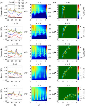
A direct comparison of the nature of shear layer vortex rollup and instabilities/pairing observed by the hot wire and stereo PIV measurements may be made via figure 4(c), which shows representative instantaneous fields of
 ${\it\omega}_{y}$
vorticity, normalized by
 $U_{j}/D$
. The agreement here is excellent; for all cases, the locations along the upstream shear layer at which the initial onset of the instabilities became apparent in the hot-wire spectrum correspond quite well with the initial shear layer vorticity rollup locations in the PIV measurements. At
 $J=41$
, the initially laminar shear layer began to roll up on its upstream side at approximately
 $z/D=2.0{-}2.5$
, consistent with the initiation of the shear layer instability in the hot-wire measurements at approximately
 $s/D=2.0$
. Beyond
 $z/D\approx 3.0$
for this flow condition, vortices on the upstream and downstream sides of the jet were observed to pair and merge, eventually breaking down into a turbulent free shear layer. This behaviour was also demonstrated by the growth of a subharmonic peak in the hot-wire power spectrum (near
 $\mathit{St}=0.38$
) at approximately
 $s/D=3.0$
. Similar agreement was found for the other momentum flux ratios in the convectively unstable regime,
 $J=20$
and
 $J=12$
.
At each of these successively lower momentum flux ratios, the location of shear layer rollup and subsequent vortex pairing moved closer to the jet exit, and the spacing between adjacent vortices was reduced, consistent with an increasing oscillation frequency of the shear layer. At
 $J=8$
, which created shear layer conditions at which the flow was globally unstable according to hot-wire measurements, little evidence of vortex pairing was seen in the PIV-based vorticity field. A distinct spacing between adjacent shear layer vortex structures was maintained for a considerable distance downstream along the upstream layer, before eventual turbulent breakdown took place. This nearly constant vortex spacing was consistent with self-excitation of the jet shear layer at a pure-tone frequency observed here and in prior hot-wire-based equidensity JICF shear layer studies (Megerian et al.
Reference Megerian, Davitian, Alves and Karagozian2007; Davitian et al.
Reference Davitian, Getsinger, Hendrickson and Karagozian2010). This spacing also increased when
 $J$
was lowered to 2, consistent with hot-wire-based trends suggesting a lowered frequency of oscillation at lower momentum flux ratios under absolutely unstable conditions. Near-immediate shear layer rollup seen in the vorticity field image for
 $J=2$
was also consistent with detection of the strong absolute instability via the hot-wire probe. We note that the strongly periodic vortex rollup shown in figure 4(c) at low momentum flux ratios (
 $J=2$
and 8) was quite similar to that observed via smoke streaklines for
 $J=4$
and
 $\mathit{Re}_{j}=7600$
by Fric & Roshko (Reference Fric and Roshko1988).
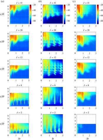
Stability characteristics for straight-pipe-generated transverse jets have not been studied to any significant degree, as noted previously. Figure 5 shows the power spectra measured along the upstream shear layer via hot-wire anemometry for the JICF injected from the flush pipe (5
a), with a fixed Reynolds number and unity density ratio, and with successively decreasing values of
 $J$
. Corresponding spectra at the same flow conditions for the flush nozzle and elevated nozzle are shown in figures 5(b) and 5(c), respectively, for comparison. Again, with a fixed set of jet conditions (
 $S$
,
 $\mathit{Re}_{j}$
), lowering
 $J$
corresponds to increasing the crossflow velocity
 $U_{\infty }$
, hence for each flow condition given in figure 5, bulk jet and free-stream crossflow velocities are virtually the same among the three injectors.
Contour plots of upstream shear layer spectral characteristics with
 $\mathit{Re}_{j}=1900$
and density ratio
 $S=1.0$
: (a) flush straight pipe injector; (b) flush nozzle injector; and (c) elevated nozzle injector. Data are shown for varying momentum flux ratios
 $J=41$
, 20, 12, 8, and 2.
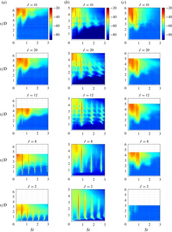
At higher momentum flux ratios corresponding to
 $J\geqslant 12$
, the flush-pipe-generated jet was observed to have considerably weaker shear layer instabilities compared with the flush-nozzle-generated JICF. The frequency-shifting tonal interactions with the hot-wire probe, observed for both the flush- and elevated-nozzle-generated JICF (and not for free jets), were completely absent for the flush-pipe-generated JICF. As documented in prior experiments (Megerian et al.
Reference Megerian, Davitian, Alves and Karagozian2007), the significant deflection of the flush-nozzle-injected jet by crossflow (as
 $U_{\infty }$
was increased), and the attendant increase in the flush nozzle upstream jet momentum thickness at injection, contributed to the stronger, more rapidly initiated convective shear layer instability observed at
 $J\geqslant 12$
in figure 5. Linear stability analysis of the flush-nozzle-generated JICF (Alves, Kelly & Karagozian Reference Alves, Kelly and Karagozian2008) predicts the variation of spatial growth rates as well as initial Strouhal numbers with decreasing
 $J$
in the range
 $J>10$
; these predictions compare well, both qualitatively and quantitatively, with experimental findings as initial jet momentum thickness increases. The flush pipe, however, already had a fully developed velocity profile and thus a large initial jet momentum thickness in the absence of crossflow; hence increasing
 $U_{\infty }$
in the range
 $J\geqslant 12$
in the present experiments appeared to have relatively little effect on the shear layer spectra.
Remarkably, as the momentum flux ratio for the flush pipe was reduced below 10 in figure 5, the flush-pipe-generated upstream shear layer exhibited strong instabilities initiated very close to the jet exit, with clear higher harmonics and weakening subharmonic modes, as did the flush nozzle. Such spectral changes suggested a rather abrupt transition to absolute instability occurring near
 $J\approx 10$
in the flush pipe, the same condition as for shear layer transition in the flush nozzle. For the two flush injectors, each set of flow parameters in figure 5 produced the same crossflow conditions to which the jet was exposed, consisting of a Blasius boundary layer adjacent to the injection wall. The fact that the transition to absolute instability for the flush pipe and flush nozzle appeared to occur at similar momentum flux ratios was likely to be was related to the strong crossflow deflecting and entering into the upstream side of the jet exit itself, as determined in numerical simulations of the flush-nozzle-generated transverse jet (Mahesh & Iyer Reference Mahesh and Iyer2013). The present diagnostics (e.g. PIV in figure 4) were not able to visualize flow within the jet nozzle or pipe, however, so this phenomenon could not be verified in the present experiments.
The elevated-nozzle-generated JICF shown in figure 5(c) exhibited similar shear layer characteristics to those of the flush nozzle for higher momentum flux ratios (
 $J\gtrsim 20$
), as observed previously. But as documented in Megerian et al. (Reference Megerian, Davitian, Alves and Karagozian2007) at lower
 $J$
values and thus higher crossflow velocities, the magnitude of vertical velocity exterior to the upstream side of the elevated nozzle increased, creating coflow which is known to stabilize a jet shear layer (Jendoubi & Strykowski Reference Jendoubi and Strykowski1994). For the range of flow conditions shown in figure 5, the elevated jet did not exhibit a transition to absolute instability, principally due to the influence of this coflow, although prior studies indicate that transition may indeed occur after the elevated jet is deflected substantially by crossflow, for
 $J\lesssim 0.93$
.
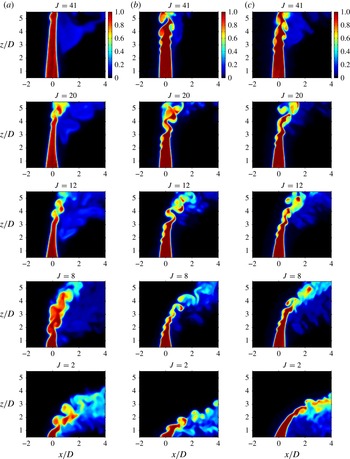
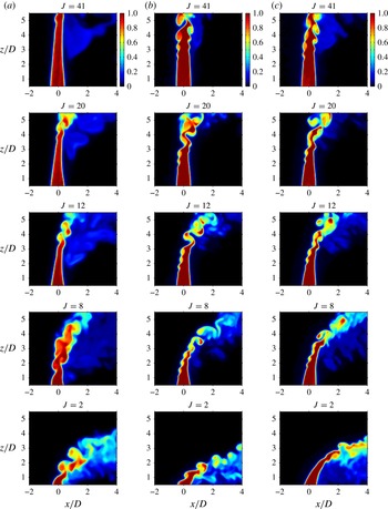
Figure 6 shows instantaneous near-field centreplane acetone PLIF concentration fields corresponding to the flow conditions for the spectral data in figure 5, for all three injectors. As with the PIV vorticity fields, the initial upstream shear layer vorticity rollup in these PLIF measurements corresponded well to the initiation of instabilities quantified in figure 5. Interestingly, while there was initiation of vortex rollup relatively close to the exit plane of the flush-pipe-generated JICF for
 $J<10$
, it showed larger and less organized vortical structures than exhibited by the flush nozzle, which had strong periodic vorticity generation and a relative lack of vortex interactions for
 $J<10$
. Thus, while the pipe-generated JICF appeared to become absolutely unstable in the same flow regime as the flush-nozzle-generated JICF, differences in the jet exit conditions did appear to cause near-field jet structural differences at all momentum flux ratios explored here.
Centreplane (side) instantaneous acetone concentration fields of the JICF near field with
 $\mathit{Re}_{j}=1900$
and density ratio
 $S=1.0$
: (a) flush straight pipe injector; (b) flush nozzle injector; and (c) elevated nozzle injector. Data are shown for varying momentum flux ratios
 $J=41$
, 20, 12, 8, and 2.
3.2. Transverse jet cross-sectional characteristics
To determine the impact of the stability characteristics of the upstream shear layer on the overall jet structure (in particular on the formation of the CVP), a detailed examination utilizing JICF
 $yz$
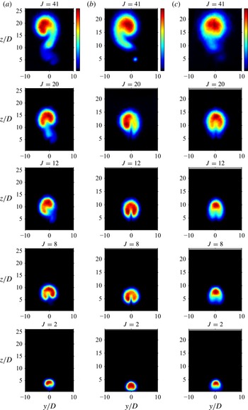
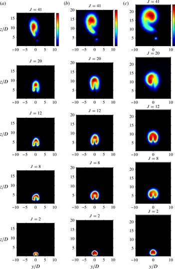
-planar imaging was undertaken for all three injectors. Figure 7 shows ensemble-averaged acetone PLIF concentration fields obtained in cross-sectional slices of the flush-nozzle-generated JICF at a fixed location
 $x/D=10.5$
downstream of injection. These images were averaged over 300 instantaneous flowfield snapshots, and are shown for the same flow conditions as in figures 5 and 6, and thus may be compared. For each average
 $yz$
-plane PLIF image, the concentration scale ranges from zero to the maximum value within each image, and thus actual concentration values may not be compared between these images (and in fact the concentration values are not indicated). The intention is that a comparison amongst the shapes of the jet cross-sections may be enabled, rather than an analysis of concentration decay and mixedness as the various jets evolve downstream, which is the focus of ongoing study.
Cross-sectional jet slices at
 $x/D=10.5$
, visualized via acetone PLIF, with
 $\mathit{Re}_{j}=1900$
and density ratio
 $S=1.0$
, averaged over 300 images: (a) flush straight pipe injector; (b) flush nozzle injector; and (c) elevated nozzle injector. A linear colourmap is used. Data are shown for varying momentum flux ratios
 $J=41$
, 20, 12, 8, and 2.
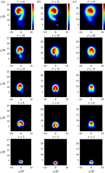
At
 $x/D=10.5$
, there were a number of flow conditions for which the jet cross-section was asymmetric and/or without a typical CVP shape. The asymmetric cases appeared for all three injectors at larger momentum flux ratios (
 $J=41$
), cases in which the upstream shear layer was found to be convectively unstable and, as documented in Megerian et al. (Reference Megerian, Davitian, Alves and Karagozian2007) for both nozzles, more susceptible to the effects of small disturbances than were jets with absolutely unstable shear layers at lower values of
 $J$
. The flush nozzle asymmetric mean cross-section also included the presence of a tertiary vortical structure below the main jet structure, similar to structures observed by Kuzo (Reference Kuzo1995) and Shan & Dimotakis (Reference Shan and Dimotakis2006). For the flush pipe at
 $J=41$
, even though its shear layer instability magnitude was weaker than that for the flush nozzle (figure 5), with relatively delayed initial shear layer rollup (figure 6), the mean jet cross-section downstream of injection also appeared to resemble a distorted, asymmetric CVP. In contrast, for smaller values of
 $J$
, especially for the flush injection and/or for which the shear layer was absolutely unstable, according to figure 5, an essentially symmetric CVP was observed. Such mean structures were seen for both flush pipe and flush nozzle cases at
 $J\leqslant 8$
, and for the flush nozzle at
 $J=12$
, a condition for which shear layer rollup and vorticity initiation appeared considerably stronger than for larger
 $J$
values.
For the elevated nozzle cases, none of the flow conditions in figure 7 appeared to create a clear cross-sectional CVP structure, except for the
 $J=20$
condition, which had similar shear layer instability and rollup features to those of the flush nozzle at this flow condition (figures 5 and 6). It should be noted that the principal difference in flow conditions between elevated and flush nozzles at
 $J=20$
was that the elevated jet was injected outside of the wall (crossflow) boundary layer and, in addition, that there was a low level of vertical coflow upstream of the elevated jet. This vertical coflow velocity was approximately 5 % of the peak jet velocity at
 $J\approx 20$
, according to the equidensity measurements for this Reynolds number regime in Megerian et al. (Reference Megerian, Davitian, Alves and Karagozian2007). This degree of coflow increased for
 $J<20$
and thus affected shear layer spectra, weakening the instabilities, as indicated in figures 5 and 6. Instantaneous concentration fields for the cross-sections of the elevated-nozzle-based JICF, especially at the higher value of
 $J=41$
, did show a temporal deflection of the jet cross-section to one side or the other about the
 $y=0$
plane. While there was sufficient positive and negative oscillation in the
 $y$
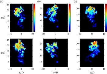
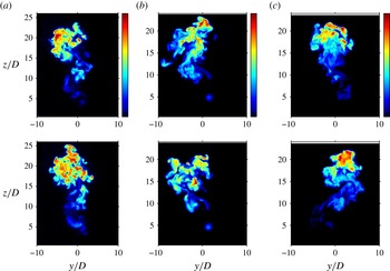
direction as to produce a somewhat more symmetric-looking jet structure in the mean, instantaneous cross-sectional images for the flush injectors at
 $J=41$
appeared to prefer one orientation, producing the more skewed image in the mean. Sample instantaneous cross-sectional images for all three injectors at
 $J=41$
are shown in figure 8.
Instantaneous cross-sectional jet slices at
 $x/D=10.5$
and at two distinct times (upper and lower images), visualized via acetone PLIF. Here
 $\mathit{Re}_{j}=1900$
and density ratio
 $S=1.0$
: (a) flush straight pipe injector; (b) flush nozzle injector; and (c) elevated nozzle injector. A linear colourmap is used. Data are shown for momentum flux ratio
 $J=41$
.
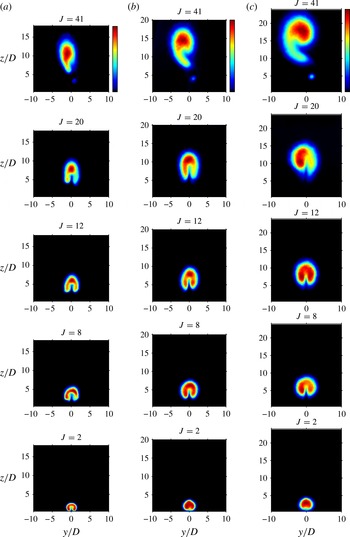
The structural asymmetry/symmetry for given flow conditions was observed from the near field of the jet and persisted downstream, as shown, for example, in figure 9 for the flush nozzle at downstream locations
 $x/D=2.5$
, 5.5, and 10.5. Those conditions producing mean structural asymmetry in the far field, e.g. for
 $J=41$
at
 $x/D=10.5$
, also showed an asymmetric structure, even with a tertiary vortex, very close to injection. Although the cross-sectional asymmetry for the flush nozzle at
 $J=20$
was greatly reduced in the near field as compared with the other clearly convectively unstable case,
 $J=41$
, the flow condition did not produce the more cleanly symmetric CVP structures in the cross-section as observed for the cases that had absolutely unstable upstream shear layers (
 $J=8$
and 2), or those with significant near-field shear layer rollup close to absolutely unstable conditions (
 $J=12$
). Extensive modifications were made to the present injection system in an attempt to eliminate these asymmetries at higher
 $J$
values. Additional flow straighteners upstream of the nozzle or pipe, an additional length of upstream pipe, rotation of the four-way injection system and even elimination of some of the orifices in the four-way system, as well as other alterations, were all tested. None had any significant effect on the mean jet cross-sectional shapes shown in figures 7 and 9. These results showed a consistent (and repeatable) correspondence between strong upstream shear layer rollup and formation of a symmetric CVP, while asymmetric cross-sectional structures corresponded to higher
 $J$
values and thus to convectively unstable shear layer conditions.
Evolution of cross-sectional jet slices of the flush-nozzle-generated JICF, visualized via acetone PLIF, with
 $\mathit{Re}_{j}=1900$
and density ratio
 $S=1.0$
, averaged over 300 images at different downstream locations: (a)
 $x/D=2.5$
; (b)
 $x/D=5.5$
; and (c)
 $x/D=10.5$
. Data are shown for varying momentum flux ratios
 $J=41$
, 20, 12, 8, and 2.
In the above cases for a fixed jet Reynolds number and density ratio, and with successively reduced momentum flux ratio
 $J$
(figures 5–7), the crossflow velocity
 $U_{\infty }$
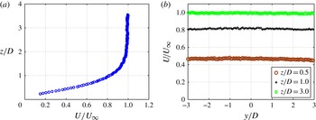
was necessarily increased. To explore the separate influence of the crossflow on jet structure, hot-wire-based tunnel boundary layer measurements were made at a location five diameters upstream of the jet orifice, in the absence of jet flow. These showed a clear laminar Blasius velocity profile for the full range of crossflow conditions. Yet at very low crossflow velocities, corresponding to the highest momentum flux ratio case in the above-noted figures, a very small degree of crossflow asymmetry in the spanwise (
 $y$
) direction was detected within the wall boundary layer.
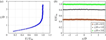
Figure 10 shows a sample upstream wall boundary layer (velocity) profile for
 $U_{\infty }=1.01\ \text{m}\ \text{s}^{-1}$
, corresponding to
 $J=41$
for the
 $\mathit{Re}_{j}=1900$
, equidensity (
 $S=1.0$
) condition. A small asymmetry across the spanwise distance
 $-3.0\leqslant y/D\leqslant 3.0$
was detected in the magnitude of local crossflow velocity within the boundary layer at an elevation of
 $z/D=0.5$
and at 5 diameters upstream of the flush orifice (
 $x/D=-5.0$
). This spanwise asymmetry in local crossflow velocity virtually disappeared beyond the edge of the wall boundary layer, above
 $z/D=3.0$
, where the percentage deviation in the local velocity across the spanwise length shown, 1.7 %, was only slightly higher than the documented uncertainty in the measurement (1.2 % of
 $U_{\infty }=1.01\ \text{m}\ \text{s}^{-1}$
, according to Megerian et al.
Reference Megerian, Davitian, Alves and Karagozian2007). The degree of crossflow asymmetry within the boundary layer, at
 $z/D=0.5$
, was a proportionately larger fraction of the local velocity, with a percentage deviation of approximately 7.3 % in the spanwise direction. Yet precision uncertainties in this single-component hot-wire-based velocity measurement at very low velocities, near the tunnel injection wall, were also higher than at the boundary layer edge, based on trends in Megerian et al. (Reference Megerian, Davitian, Alves and Karagozian2007). At free-stream crossflow velocities exceeding
 $U_{\infty }=1.01\ \text{m}\ \text{s}^{-1}$
, the spanwise asymmetries within the wall boundary layer were typically smaller than those documented in figure 10, although a complete study of the crossflow boundary layer for all flow conditions was not conducted.
Crossflow boundary layer velocity measurements via hot wire: (a) velocity profile upstream of the jet nozzle, at
 $x/D=-5.0$
and
 $y/D=0$
; (b) local streamwise velocity measured at several different locations relative to the tunnel wall (
 $z/D=0.5,1.0,3.0$
) at
 $x/D=-5.0$
with variable spanwise location
 $y/D$
. Conditions correspond to crossflow velocity in the free stream
 $U_{\infty }=1\ \text{m}\ \text{s}^{-1}$
, with the jet flow turned off.
An examination of the effect of this or any undetected asymmetry associated with the crossflow was conducted at a fixed value of
 $U_{\infty }=1.01\ \text{m}\ \text{s}^{-1}$
, while varying the jet Reynolds number, and thereby also varying the momentum flux ratio. By fixing the crossflow conditions, one essentially fixes any asymmetric properties that the crossflow may have had at
 $U_{\infty }=1.01\ \text{m}\ \text{s}^{-1}$
while exploring jet responses under different injection conditions (different injectors and flow conditions), and thus, for different jet shear layer stability characteristics. At a fixed downstream location
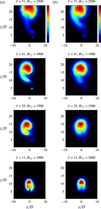
 $x/D=10.5$
, averaged
 $yz$
-plane PLIF images for the flush nozzle are shown in figure 11(a); here jet fluid was injected directly into the incoming crossflow boundary layer (and hence into an upstream separation region created by the jet interaction with crossflow, according to Kelso & Smits Reference Kelso and Smits1995 and Kelso et al.
Reference Kelso, Lim and Perry1996). Mean cross-sectional images for the elevated nozzle, where the jet was injected above/outside of the wall boundary layer, are shown in figure 11(b).
Cross-sectional jet slices (location
 $x/D=10.5$
) visualized via acetone PLIF, with fixed
 $U_{\infty }=1.01\ \text{m}\ \text{s}^{-1}$
, density ratio
 $S=1.0$
, averaged over 300 images: (a) flush nozzle injector; and (b) elevated nozzle injector. Data are shown for varying momentum flux ratios and jet Reynolds numbers as given.
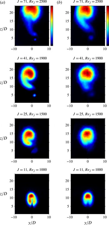
For the flush nozzle in figure 11(a), at higher momentum flux ratios and Reynolds numbers (
 $J\geqslant 25$
and
 $\mathit{Re}_{j}\geqslant 1500$
) for which present and prior studies showed a convectively unstable shear layer and delayed shear layer vorticity rollup, the jet cross-sections were quite asymmetric, with a skewed CVP structure. For
 $J=11$
, however, the jet cross-section became much more symmetric for the flush-nozzle-generated jet, with a CVP structure appearing at conditions typically approaching an absolutely unstable upstream shear layer.
For the elevated nozzle cases in figure 11(b), most of the flow conditions shown produced somewhat more symmetric jet cross-sections, although none corresponded to a clear, symmetric CVP. At very high values of
 $J=71$
and
 $\mathit{Re}_{j}=2500$
, the asymmetry for the elevated nozzle was rather pronounced, and was similar to the asymmetric CVP for the flush nozzle at the same conditions. According to data in Megerian et al. (Reference Megerian, Davitian, Alves and Karagozian2007), at
 $J\approx 71$
in this Reynolds number range, the degree of vertical coflow upstream of the elevated nozzle is quite small, less than 3 % of the peak jet velocity at the nozzle exit plane. Hence the shear layer spectral characteristics were virtually identical between the flush and elevated nozzles under these conditions. The only other difference in flow conditions between the two nozzles at
 $J=71$
was the very small spanwise crossflow asymmetry to which the flush-nozzle-injected jet may have been exposed, compared with a slightly more symmetric free-stream crossflow for the elevated nozzle (figure 10). Neither of these effects appeared to have a substantial effect on altering the degree of cross-sectional asymmetry at
 $J=71$
.
For the elevated nozzle at lowered values of
 $J$
and
 $\mathit{Re}_{j}$
in figure 11, all of which produced successively weaker shear layer instabilities due to the increasing external vertical coflow, there were few conditions that actually produced a CVP shape in the mean, although the cross-sections became more symmetric at lower
 $J$
values. As noted previously for the elevated jet in figure 7, instantaneous images showed there was a deflection of the jet cross-section to one side or the other in the
 $y$
direction, with sufficient flipping back and forth in time as to produce a generally symmetric jet structure in the mean, but without the distinctive CVP shape. The weakening upstream shear layer instabilities for the elevated nozzle with reduced
 $J$
, documented here and in previous studies (Megerian et al.
Reference Megerian, Davitian, Alves and Karagozian2007), corresponded to the jet lessened ability to sustain shear layer vorticity rollup and thus form a clear CVP for
 $J\lesssim 41$
. Hence it is likely that these weakened shear layer instabilities for the elevated nozzle, rather than the small spanwise asymmetries in crossflow boundary layer profiles, produced the differences between flush and elevated nozzle mean cross-sectional images observed in figure 11. But the fact that the crossflow conditions upstream of jet injection were the same for all images shown in figure 11 suggested that it was the response of the transverse jet to the crossflow, and not the crossflow in and of itself, that created different jet flow structures. The cross-sectional asymmetries were most strongly correlated with the nature of jet shear layer instabilities, as created by differing injectors and momentum flux ratios.
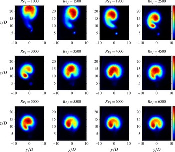
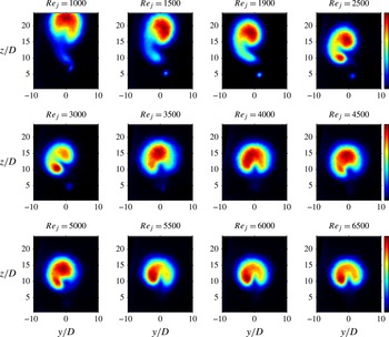
Other researchers have observed that the jet Reynolds number itself could have a degree of influence on jet cross-sectional symmetry (Kuzo Reference Kuzo1995; Shan & Dimotakis Reference Shan and Dimotakis2006). For a fixed value of
 $J=41$
and variable jet Reynolds numbers
 $1000\leqslant \mathit{Re}_{j}\leqslant 6500$
, shown in figure 12 for the flush nozzle, the present studies showed that the jet cross-section was indeed asymmetric, with the presence of a tertiary vortex structure, for lower Reynolds numbers in the range
 $\mathit{Re}_{j}\lesssim 3500$
. Transverse jets in this lower Reynolds number range have been documented (Megerian et al.
Reference Megerian, Davitian, Alves and Karagozian2007) to produce convectively unstable shear layers. At Reynolds numbers above 3500, the transverse jet cross-section became generally more symmetric in figure 12, with mean shapes that were closer to the expected CVP and without the tertiary vortical structure. Unequal distributions of jet fluid did appear to be present on either side of the CVP-like structures for such conditions, however. In fact, the slightly asymmetric CVP structure at
 $\mathit{Re}_{j}\gtrsim 5500$
and
 $J=41\ (R=6.4)$
was similar to that observed at
 $\mathit{Re}_{j}=5000$
and
 $R=6$
in the experiments of Narayanan et al. (Reference Narayanan, Barooah and Cohen2003) and in the corresponding simulations of Muldoon & Acharya (Reference Muldoon and Acharya2010), and is reminiscent of cross-sectional structures observed at higher Reynolds numbers and momentum flux ratios by Smith & Mungal (Reference Smith and Mungal1998).
Cross-sectional jet slices at location
 $x/D=10.5$
, visualized via acetone PLIF, with fixed
 $J=41$
and density ratio
 $S=1.0$
, averaged over 300 images for the flush-nozzle-generated jet. A linear colourmap is used. Data are shown for varying jet Reynolds numbers as indicated.
The transition in cross-sectional structure to the more symmetric CVP for a fixed density ratio
 $S$
and reduced momentum flux ratio
 $J$
was also observed when
 $S$
was reduced below unity, with fixed
 $J$
and
 $\mathit{Re}_{j}$
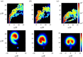
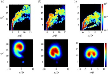
. Figure 13 shows instantaneous centreplane and mean cross-sectional concentration fields of the JICF for
 $J=41$
and
 $\mathit{Re}_{j}=1900$
, but with successively reduced density ratios. When
 $S\lesssim 0.40$
, the jet shear layer becomes absolutely unstable, as documented in Getsinger et al. (Reference Getsinger, Hendrickson and Karagozian2012). Centreplane concentration fields in figure 13 showed, for absolutely unstable shear layer conditions (
 $S=0.35$
), a relatively rapid initiation of strong shear layer vorticity, and these in turn produced a more symmetric CVP-like cross-sectional structure in the mean, albeit with some persistence of a lower vortical structure evolving downstream which was visible in the mean cross-sectional image. At higher density ratios in figure 13, for which upstream shear layers were documented to be convectively unstable, the cross-sectional shapes were much more asymmetric. Hence overall for the low density JICF, as for the equidensity JICF, there was a correspondence between near-field jet shear layer instabilities (and the associated vorticity rollup) and the degree of symmetry in the CVP structure dominating the jet mean cross-sectional shape.
Instantaneous centreplane acetone concentration fields (top row) and mean cross-sectional jet slices (bottom row) at location
 $x/D=10.5$
, visualized via acetone PLIF with fixed
 $J=41$
and jet Reynolds number
 $\mathit{Re}_{j}=1900$
. A logarithmic colourmap is used for centreplane images, and a linear colourmap is used for cross-sectional images. Data are shown for varying jet-to-crossflow density ratios: (a)
 $S=1.0$
, (b)
 $S=0.55$
, (c)
 $S=0.35$
.
4. Discussion and conclusions
The present experimental results provide a systematic assessment of the effects of transverse jet injection configuration, momentum flux ratio, Reynolds number, and density ratio on shear layer stability characteristics and the resulting jet structure. Both PIV and acetone PLIF images provided evidence that the strengthening shear layer instabilities and transition from convective to absolute instability observed at lowered momentum flux ratios and/or lowered jet-to-crossflow density ratios were associated with increasingly strong, near-field periodic shear layer vorticity rollup. While this correspondence was not unexpected, the fact that the flush-pipe-generated jet shear layer transition, from a rather weak convective instability to absolute instability, occurred at approximately the same flow conditions (
 $J\approx 10$
) as for the flush nozzle was somewhat unexpected. For both flush injection configurations there was similarly rapid upstream shear layer vorticity rollup for absolutely unstable conditions, suggesting similar mechanisms for this transition between the two flush injectors. These mechanisms are currently under examination by our group and others (Mahesh & Iyer Reference Mahesh and Iyer2013).
The comparisons in jet cross-sectional structure for various injectors and flow conditions in figures 7, 11, and 13 all suggested that the state of the upstream shear layer instabilities, and thus the strength of shear layer vorticity rollup, were most closely associated with the degree of symmetry or asymmetry in the mean transverse jet cross-section. In these figures, the clearest correspondence for the formation of a symmetric CVP was with lower momentum flux ratios and/or low jet-to-crossflow density ratios, each producing absolutely unstable shear layers and rapid near-field shear layer vorticity rollup. This correspondence is consistent with the ideas of Kelso et al. (Reference Kelso, Lim and Perry1996) and Cortelezzi & Karagozian (Reference Cortelezzi and Karagozian2001), which suggest that shear layer vorticity evolution and deformation by crossflow contributes most significantly to the formation of the CVP itself.
The clearest correspondence of asymmetry and/or lack of a symmetric CVP in the jet cross-section was with a relatively weak and/or convectively unstable shear layer, typically occurring at larger momentum flux ratios and lower jet Reynolds numbers. The elevated nozzle especially weakened shear layer instabilities at lower
 $J$
, documented to occur due to increasing vertical coflow (Megerian et al.
Reference Megerian, Davitian, Alves and Karagozian2007), not only delayed or prevented a substantial rollup in vorticity, but in turn appeared to prevent the formation of a clear, symmetric CVP. The elevated nozzle cross-sections in this regime (
 $J<41$
), however, were relatively symmetric. Interestingly, at higher momentum flux ratios for all three injectors explored here, the jet mean cross-sectional shape resembled an asymmetrically skewed CVP, corresponding in all cases to a convectively unstable shear layer. Transverse jets with convectively unstable shear layers have been shown to be susceptible to small axisymmetric perturbations (Megerian et al.
Reference Megerian, Davitian, Alves and Karagozian2007), while under absolutely unstable shear layer conditions, the jet is unaffected by such axisymmetric disturbances. Numerical simulations by Muldoon & Acharya (Reference Muldoon and Acharya2010) suggest that the transverse jet at a high momentum flux ratio is susceptible to asymmetric disturbances as well, and that such asymmetric states could appear in an experiment. Small asymmetries or imperfections in the present experiment could well have been a trigger for an alteration in the jet shear layer rollup process that has long been associated with CVP formation, as discussed by Smith & Mungal (Reference Smith and Mungal1998). Based on the present results, such triggers would affect the jet natural evolution when the shear layer is susceptible to alteration, which is the case for the convectively unstable JICF, but is not the case when the shear layer is absolutely unstable.
While the notion that the CVP formation is associated with the evolution and rollup of transverse jet shear layer vorticity is not a new premise (Kelso et al. Reference Kelso, Lim and Perry1996; Cortelezzi & Karagozian Reference Cortelezzi and Karagozian2001), to our knowledge this is the first explicit demonstration of this association. The present results suggest that the converse may also be true, that is, that the CVP may be either asymmetric or nearly absent for relatively weak shear layer instability and near-field vorticity generation, as occurs in the case of a convectively unstable shear layer condition. These JICF symmetry results could be used to explain differences in observed trends in mixing metrics associated with longitudinal centreplane slices of the jet trajectory, some of which omit regions of significantly higher concentration appearing in the jet cross-section, and metrics associated with the jet cross-section, which omit consideration of downstream evolutionary aspects of jet structure, entrainment and mixing. Future experiments will examine such mixing processes and their correspondence to jet structure and instability.
Acknowledgements
The authors thank W. Y. Peng, T. Shoji, A. Sung, S. Miller, and J. Smolke for their assistance during the course of these studies. This project has been supported by the National Science Foundation under grant CBET-1133015, by the Air Force Office of Scientific Research under grant FA9550-11-1-0128 and DURIP grant FA9550-10-1-0461, and by the NASA Graduate Student Researchers Program.