

1 Introduction
The breakup of ocean waves entraps air bubbles that disintegrate within the liquid bulk and burst when they rise back to the surface, ejecting into the atmosphere droplets which, after evaporation, constitute the so-called sea spray aerosol (SSA), which influences climate by scattering and absorbing radiation and also because a fraction of the solid particles composing the SSA serve as cloud condensation nuclei and ice nuclei (de Leeuw et al. Reference de Leeuw, Andreas, Anguelova, Fairall, Lewis, O’Dowd, Schulz and Schwartz2011; Veron Reference Veron2015; Erinin et al. Reference Erinin, Wang, Liu, Towle, Liu and Duncan2019). Hence, the understanding, description and quantification of a fundamental process such as the bursting of bubbles at interfaces, which produce drops with different chemical compositions (Wang et al. Reference Wang, Deane, Moore, Ryder, Stokes, Beall, Collins, Santander, Burrows and Sultana2017) depending on whether drops are formed through the disintegration of the cap film (Lhuissier & Villermaux Reference Lhuissier and Villermaux2012) (i.e. film drops) or via the breakup of the jet ejected upwards from the base of the collapsing cavity (MacIntyre Reference MacIntyre1972) (i.e. jet drops), will help improve the predictive capability of climate models.
It is a common belief that most of the submicrometric particles composing SSA originate from film drops (Veron Reference Veron2015), but, very recently, Wang et al. (Reference Wang, Deane, Moore, Ryder, Stokes, Beall, Collins, Santander, Burrows and Sultana2017) demonstrated that the fraction of submicrometric SSA which can be attributed to jet drops varies from 20 % to 40 %, depending on the seawater chemical composition. The flux of SSA from jet drops is usually calculated using, as an intermediate step, the well-known 10 % rule, which approximates the drop radii as  $R_{d}=0.1R_{b}$, with
 $R_{b}$ the bubble radius. This approximation is commonly used and has been employed very recently in the paper by Wang et al. (Reference Wang, Deane, Moore, Ryder, Stokes, Beall, Collins, Santander, Burrows and Sultana2017). However, the numerical simulations in Duchemin et al. (Reference Duchemin, Popinet, Josserand and Zaleski2002) demonstrated, almost 20 years ago, that the function
 $R_{d}/R_{b}$ varies non-monotonically with
 $R_{b}$ and also that
 $\min (R_{d}/R_{b})\sim O(0.01)$ – a fact further confirmed by the more accurate numerical results reported in Brasz et al. (Reference Brasz, Bartlett, Walls, Flinn, Yu and Bird2018).
Then, motivated by its atmospheric and climate implications and by the remarkable findings in Wang et al. (Reference Wang, Deane, Moore, Ryder, Stokes, Beall, Collins, Santander, Burrows and Sultana2017), this contribution aims at improving the quantification of the SSA produced from jet drops. Here we make use of our theory in Gordillo & Rodríguez-Rodríguez (Reference Gordillo and Rodríguez-Rodríguez2019) and provide equations for  $R_{d}$ and for the initial velocity of the droplets ejected,
 $V_{d}$, as a function of
 $R_{b}$ and of the physical properties of the liquid. In doing so, we will also present a new model describing the spatio-temporal evolution of the jet that, among other things, predicts the behaviour of function
 $R_{d}/R_{b}$ around its minimum. Let us point out that our study is limited to the range of bubble diameters of interest for SSA production, for which gravitational effects can be neglected in a first approximation.
The paper is structured as follows: in § 2 we briefly describe the numerical simulations and present some of the results obtained. Section 3 is devoted to developing a model describing the spatio-temporal evolution of the jet from its inception to its breakup and to comparing our predictions with experimental and numerical results. Finally, § 4 summarizes the main results obtained.
2 Numerical set-up and revision of previous results
With the main purpose of analysing the ejection of droplets from the very fast Worthington jets ejected after the bursting of a bubble of radius  $R_{b}$, here we have performed an exhaustive numerical study by varying both the Bond and Ohnesorge numbers, respectively defined as
 $Bo=\unicode[STIX]{x1D70C}_{l}\,g\,R_{b}^{2}/\unicode[STIX]{x1D70E}$ and
 $Oh=\unicode[STIX]{x1D707}_{l}/\sqrt{\unicode[STIX]{x1D70C}_{l}\,R_{b}\,\unicode[STIX]{x1D70E}}$, with
 $\unicode[STIX]{x1D70C}_{l}$,
 $\unicode[STIX]{x1D707}_{l}$ and
 $\unicode[STIX]{x1D70E}$ referring to the liquid density, dynamic viscosity and interfacial tension coefficient, respectively (see figure 1a). Here, lengths, times and pressures are made non-dimensional by using as characteristic values
 $R_{b}$,
 $\sqrt{\unicode[STIX]{x1D70C}_{l}\,R_{b}^{3}/\unicode[STIX]{x1D70E}}$ and
 $\unicode[STIX]{x1D70E}/R_{b}$, and hence, velocities will be made non-dimensional using as the characteristic value the capillary velocity,
 $V_{c}=\sqrt{\unicode[STIX]{x1D70E}/\left(\unicode[STIX]{x1D70C}_{l}\,R_{b}\right)}$. Dimensionless variables will be written throughout the text in lower-case letters to differentiate them from their dimensional counterparts – in capitals – and the subscript
 $d$ will be used to denote quantities referring to the instant the droplet detaches from the tip of the jet.
Axisymmetric numerical simulations have been performed using the open source code GERRIS (Popinet Reference Popinet2003; Brasz et al. Reference Brasz, Bartlett, Walls, Flinn, Yu and Bird2018; Deike et al. Reference Deike, Ghabache, G., Das, Popinet and Séon2018; Gordillo & Rodríguez-Rodríguez Reference Gordillo and Rodríguez-Rodríguez2019) using as values for the density and viscosity ratios those corresponding to air bubbles in water: namely, 1. 2 × 10⁻³ and 1. 8 × 10⁻². The computations are started by suddenly removing the cap of a static bubble at a free surface. The initial shape of the bubble (see figure 1a) at  $T=0$ is calculated by solving the Young–Laplace equation for different values of the Bond number, following the procedure detailed in Lhuissier & Villermaux (Reference Lhuissier and Villermaux2012). Simulations with different grid refinements (maximum level of refinement varying from 10 to 14) have been carried out to check the grid independence of the results. We have further validated our numerics by comparing with Brasz et al. (Reference Brasz, Bartlett, Walls, Flinn, Yu and Bird2018), and the GERRIS script developed here is provided as part of the supplementary material available at https://doi.org/10.1017/jfm.2019.1061.
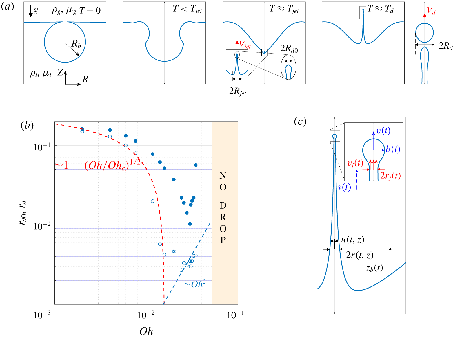
(a) Sketch showing the sequence of events following the bursting of a bubble at a free interface. The retraction of the rim causes a convergent flow towards the base of the cavity that favours the formation of a fast jet of initial velocity  $V_{jet}$ and initial radius
 $R_{jet}$. For sufficiently small values of the Ohnesorge numbers, a drop of radius
 $R_{d}$ and velocity
 $V_{d}$ is issued from the tip of the jet. (b) Numerical results for the dimensionless droplet radius at the ejection time (
 $r_{d0}$, open markers) and at the breakup time (
 $r_{d}$, filled markers) corresponding to
 $Bo=0.01$ and different values of the Ohnesorge number. (c) Sketch defining the main variables used in the model developed here to predict
 $r_{d}$ and
 $v_{d}$.

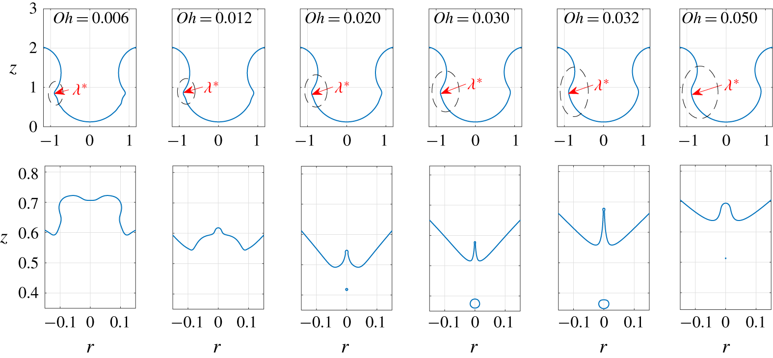
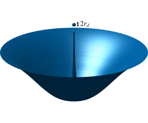
Shapes of the collapsing cavity for different values of the Ohnesorge number at two different instants of time. Observe that a tiny bubble is entrapped below the jet for  $Oh_{c}\leqslant Oh\leqslant Oh_{d}$, with
 $Oh_{c}\simeq 0.02$ and
 $Oh_{d}\simeq 0.05$. Here,
 $Bo=0.01$.

Gordillo & Rodríguez-Rodríguez (Reference Gordillo and Rodríguez-Rodríguez2019) explained that bubble bursting jets are produced by a purely inertial mechanism in which capillarity transforms the initial spherical bubble into a truncated cone, with the radius of the base of such a cone decreasing linearly with  $\unicode[STIX]{x1D706}^{\ast }$ – namely the wavelength of the capillary wave excited during the rim retraction process (see figure 2). Gordillo & Rodríguez-Rodríguez (Reference Gordillo and Rodríguez-Rodríguez2019) found, both theoretically and numerically, that
 $\unicode[STIX]{x1D706}^{\ast }\propto Oh^{1/2}$ and also that the amplitude of this wave is
 $\propto \unicode[STIX]{x1D706}^{\ast }$ for
 $Oh\lesssim 0.02$. Then, since the radius of the truncated cone varies linearly with
 $\unicode[STIX]{x1D706}^{\ast }$, it was also predicted in Gordillo & Rodríguez-Rodríguez (Reference Gordillo and Rodríguez-Rodríguez2019) that the radius of the incipient jet,
 $r_{jet}$, can be expressed as
 $$\begin{eqnarray}r_{jet}\propto 1-(Oh/Oh_{c})^{1/2},\quad \text{if }Oh<Oh_{c}(Bo)\simeq 0.02,\end{eqnarray}$$
with  $Oh_{c}(Bo)$ the value of the Ohnesorge number for which the crest of the wave reaches the vertex of the cone. Notice that
 $Oh_{c}$ depends on the Bond number because the vertex position depends on the initial shape of the static bubble, which clearly depends on the Bond number. Gordillo & Rodríguez-Rodríguez (Reference Gordillo and Rodríguez-Rodríguez2019) also explained that, for
 $Oh\lesssim Oh_{c}$, the initial velocity of the extremely fast and thin jet,
 $v_{jet}$, can be calculated as the flow generated by a continuous line of sinks extending upwards from the base of the truncated cone along the axis of symmetry a distance proportional to
 $\unicode[STIX]{x1D706}^{\ast }\propto Oh^{1/2}$. Moreover, the intensity of these sinks also depends on
 $Oh^{1/2}$ through the capillary pressure, which depends on the cone geometry. All these facts explain why
 $v_{jet}$ depends on
 $Oh^{1/2}$, with the precise functional form of
 $v_{jet}$ calculated in Gordillo & Rodríguez-Rodríguez (Reference Gordillo and Rodríguez-Rodríguez2019) as
 $$\begin{eqnarray}v_{jet}\propto Oh^{1/2},\quad \text{for }Oh\ll 1\quad \text{and}\quad v_{jet}\propto (1-(Oh/Oh_{c})^{1/2})^{-1/2},\quad \text{for }Oh\approx Oh_{c}.\end{eqnarray}$$
The shapes of the collapsing bubbles for different values of the Ohnesorge number are represented in figure 2 for two different instants of time. Observe that there is a remarkable difference between the two smaller values of  $Oh$ and
 $Oh=0.02$; in this latter case, a tiny bubble is entrapped below the jet. This bubble is created because the crest of the capillary wave reaches the vertex of the cone for
 $Oh=Oh_{c}$ and a point below the vertex for
 $Oh>Oh_{c}$. From (2.2), notice that the predicted velocity would tend to infinity for
 $Oh=Oh_{c}$, but this singularity is clearly not realistic. Indeed, it was shown in Gordillo & Rodríguez-Rodríguez (Reference Gordillo and Rodríguez-Rodríguez2019) that, when a bubble is entrapped, the jet velocity is limited by viscous stresses and, thus, the dimensional jet velocity and jet radius are respectively given by
 $V_{jet}\propto \unicode[STIX]{x1D70E}/\unicode[STIX]{x1D707}_{l}$ and
 $R_{jet}\propto \unicode[STIX]{x1D707}_{l}^{2}/(\unicode[STIX]{x1D70C}_{l}\unicode[STIX]{x1D70E})$. These are constant values for fixed physical properties and represent the maximum achievable velocity and the minimum achievable radius (with slight deviations near
 $Oh=0.03$, as will be commented below) which, in dimensionless terms, can be expressed as
 $$\begin{eqnarray}r_{jet}\propto Oh^{2}\quad \text{and}\quad v_{jet}\propto Oh^{-1}\quad \text{for }Oh>Oh_{c}.\end{eqnarray}$$
The case  $Oh=0.032$ in figure 2 illustrates a case for which (2.3) accurately predicts the numerical results. However, for the largest value of the Ohnesorge number illustrated in figure 2, the amplitude of the capillary wave is very much attenuated by viscosity. Consequently, the crests of the capillary waves do not reach the vertex of the cone for
 $Oh>Oh_{d}$, with
 $Oh_{d}(Bo\leqslant 0.01)\simeq 0.05$. Therefore, bubbles are entrapped below the jet for values of the Ohnesorge numbers within the range
 $$\begin{eqnarray}Oh_{c}(Bo)\leqslant Oh\leqslant Oh_{d}(Bo),\quad \text{with }Oh_{c}(Bo\ll 1)\approx 0.02\text{ and }Oh_{d}(Bo\ll 1)\approx 0.05.\end{eqnarray}$$
Clearly, the predictions in (2.1) and (2.2) will deteriorate as  $Oh$ approaches
 $Oh_{c}$ and, also, there will be deviations from the predictions given in (2.3) for values of
 $Oh$ near the boundaries limiting the bubble entrapment regime – namely,
 $Oh_{c}$ and
 $Oh_{d}$. In spite of this, the numerical results depicted in figure 1(b) verify the scalings in (2.1) and (2.3), confirming the non-monotonic dependence of the initial radius of the jet predicted in Gordillo & Rodríguez-Rodríguez (Reference Gordillo and Rodríguez-Rodríguez2019). Figure 1(b) also reveals that the radii of the ejected droplets,
 $r_{d}$, which is the truly important value for applications, are far larger than their initial value,
 $r_{d0}$.
Our goal in this contribution is to provide closed expressions for  $r_{d}$ and
 $v_{d}$ at the instant the top droplet is emitted from the tip of the jet. For that purpose, we will derive a system of differential equations that will be integrated making use of the initial values for the jet radius and the jet velocity, which can be either calculated numerically or approximated using (2.1), (2.2) and (2.3). However, to do so, it will be first necessary to describe the spatio-temporal evolution of the jet width and of the jet velocity upstream the jet tip.
3 Modelling the spatio-temporal evolution of the jet
The time evolution of the jet tip velocity,  $v(t)$, and of the radius of curvature of the tip of the jet,
 $b(t)$, can be calculated using the following mass and momentum balances (Taylor Reference Taylor1959):
 $$\begin{eqnarray}\left.\begin{array}{@{}c@{}}{\displaystyle \frac{\text{d}s}{\text{d}t}}=v,\quad {\displaystyle \frac{4}{3}}\unicode[STIX]{x03C0}{\displaystyle \frac{\text{d}b^{3}}{\text{d}t}}=\unicode[STIX]{x03C0}r_{j}^{2}(v_{j}-v),\\ {\displaystyle \frac{4}{3}}\unicode[STIX]{x03C0}b^{3}{\displaystyle \frac{\text{d}v}{\text{d}t}}=-\unicode[STIX]{x03C0}r_{j}+\unicode[STIX]{x03C0}r_{j}^{2}(v-v_{j})^{2}-6\unicode[STIX]{x03C0}Oh\left({\displaystyle \frac{\unicode[STIX]{x1D707}_{g}}{\unicode[STIX]{x1D707}_{l}}}\right)bv,\end{array}\right\}\end{eqnarray}$$
with  $r_{j}(t)=r(s(t),t)$ and
 $v_{j}(t)=u(s(t),t)$ the values of the radius
 $r(z,t)$ and of the vertical component of the liquid velocity
 $u(z,t)$ at the vertical position
 $z=s(t)$ where a drop of radius
 $b(t)$ is located (see figure 1c). In (3.1), notice that the dimensionless term,
 $-\unicode[STIX]{x03C0}r_{j}$, results from the addition of two contributions: the interfacial tension force along the perimeter of a circle of radius
 $r_{j}$,
 $-2\unicode[STIX]{x03C0}r_{j}$, plus the force
 $\unicode[STIX]{x03C0}r_{j}$ associated with the capillary pressure
 $1/r_{j}$ exerted on a circle of area
 $\unicode[STIX]{x03C0}\,r_{j}^{2}$. Equations (3.1) express that the jet tip is mainly decelerated by the action of interfacial tension forces, but we have also added the small force exerted by the gas because we checked that the inclusion of the Stokes drag over a sphere of radius
 $b(t)$, with
 $\unicode[STIX]{x1D707}_{g}$ in (3.1) the gas viscosity, slightly improves the agreement between the numerical results and the model.
Clearly, the system (3.1) can only be solved once  $r_{j}(t)$ and
 $v_{j}(t)$ are known. For that purpose, here we make use of the ballistic equations for
 $r(z,t)$ and
 $u(z,t)$ in the form presented in Gekle & Gordillo (Reference Gekle and Gordillo2010):
 $$\begin{eqnarray}\left.\begin{array}{@{}c@{}}{\displaystyle \frac{\unicode[STIX]{x2202}r^{2}}{\unicode[STIX]{x2202}t}}+{\displaystyle \frac{\unicode[STIX]{x2202}}{\unicode[STIX]{x2202}z}}(r^{2}\,u)=0\Rightarrow {\displaystyle \frac{\text{D}}{\text{D}t}}(\ln r^{2})=-S,\quad \text{with }S={\displaystyle \frac{\unicode[STIX]{x2202}u}{\unicode[STIX]{x2202}z}}\quad \text{and}\\[12.0pt] {\displaystyle \frac{\unicode[STIX]{x2202}u}{\unicode[STIX]{x2202}t}}+u{\displaystyle \frac{\unicode[STIX]{x2202}u}{\unicode[STIX]{x2202}z}}=0\Rightarrow {\displaystyle \frac{\text{D}u}{\text{D}t}}=0,\end{array}\right\}\end{eqnarray}$$
with  $\text{D}/\text{D}t\equiv \unicode[STIX]{x2202}/\unicode[STIX]{x2202}t+u\,\unicode[STIX]{x2202}/\unicode[STIX]{x2202}z$ indicating the material derivative and
 $S$ the strain rate.
The parabolic system of (3.2) can be solved using the method of characteristics in the spatio-temporal region  $s(t)\geqslant z\geqslant z_{b}(t)$, with
 $z_{b}(t)$ the origin of the ballistic region. The solution can be found once the liquid velocity and the jet radius
 $u(\unicode[STIX]{x1D70F},z_{b}(\unicode[STIX]{x1D70F}))=u_{b}(\unicode[STIX]{x1D70F})$ and
 $r(\unicode[STIX]{x1D70F},z_{b}(\unicode[STIX]{x1D70F}))=r_{b}(\unicode[STIX]{x1D70F})$ are known functions of time at the spatio-temporal boundary
 $(\unicode[STIX]{x1D70F},z_{b}(\unicode[STIX]{x1D70F}))$. Indeed, the integration of the momentum equation in (3.2) yields that along rays
 $z=z_{b}(\unicode[STIX]{x1D70F})+(t-\unicode[STIX]{x1D70F})\,u_{b}(\unicode[STIX]{x1D70F})$ the liquid velocity is
 $u=u_{b}(\unicode[STIX]{x1D70F})$. Moreover, to integrate the continuity equation in (3.2) it is first convenient to notice that
 $$\begin{eqnarray}\frac{\unicode[STIX]{x2202}}{\unicode[STIX]{x2202}z}\left(\frac{\unicode[STIX]{x2202}u}{\unicode[STIX]{x2202}t}+u\frac{\unicode[STIX]{x2202}u}{\unicode[STIX]{x2202}z}\right)=0\Rightarrow \frac{\text{D}S}{\text{D}t}+S^{2}=0\Rightarrow -\frac{\text{D}S}{S^{2}}=\text{D}t\Rightarrow S=\frac{S_{b}(\unicode[STIX]{x1D70F})}{1+\left(t-\unicode[STIX]{x1D70F}\right)S_{b}(\unicode[STIX]{x1D70F})},\end{eqnarray}$$
with (see Gekle & Gordillo Reference Gekle and Gordillo2010)
 $$\begin{eqnarray}S_{b}(\unicode[STIX]{x1D70F})=\frac{\unicode[STIX]{x2202}u}{\unicode[STIX]{x2202}z}(\unicode[STIX]{x1D70F},z_{b}(\unicode[STIX]{x1D70F}))=-\frac{\text{d}u_{b}/\text{d}\unicode[STIX]{x1D70F}}{u_{b}(\unicode[STIX]{x1D70F})-\text{d}z_{b}/\text{d}\unicode[STIX]{x1D70F}}.\end{eqnarray}$$
Therefore, the substitution of (3.4) into the continuity equation in (3.2) yields
 $$\begin{eqnarray}\frac{\text{D}}{\text{D}t}(\ln r^{2})=-\frac{S_{b}(\unicode[STIX]{x1D70F})}{1+(t-\unicode[STIX]{x1D70F})S_{b}(\unicode[STIX]{x1D70F})}\Rightarrow r=\frac{r_{b}(\unicode[STIX]{x1D70F})}{\sqrt{1+(t-\unicode[STIX]{x1D70F})S_{b}(\unicode[STIX]{x1D70F})}}.\end{eqnarray}$$
The inertio-capillary balance existing for values of the Ohnesorge number  $Oh\sim Oh_{c}$ (Gordillo & Rodríguez-Rodríguez Reference Gordillo and Rodríguez-Rodríguez2019) during a short interval of time after the jet is ejected causes the time evolution of the jet to be self-similar (Zeff et al. Reference Zeff, Kleber, Fineberg and Lathrop2000; Brasz et al. Reference Brasz, Bartlett, Walls, Flinn, Yu and Bird2018; Lai, Eggers & Deike Reference Lai, Eggers and Deike2018) – a fact yielding that the liquid velocity and the jet radius at
 $z_{b}(\unicode[STIX]{x1D70F})$ can be respectively expressed as
 $u_{b}(\unicode[STIX]{x1D70F})=u_{0}\,\unicode[STIX]{x1D70F}^{-1/3}$ and
 $r_{b}(\unicode[STIX]{x1D70F})=r_{0}\,\unicode[STIX]{x1D70F}^{2/3}$. Defining the origin of the jet region at the vertical position
 $z_{b}(\unicode[STIX]{x1D70F})=u_{0}\,\unicode[STIX]{x1D70F}^{2/3}$, making use of (3.4) and of the fact that
 $u_{b}(\unicode[STIX]{x1D70F})=u_{0}\,\unicode[STIX]{x1D70F}^{-1/3}$ and that
 $z=z_{b}(\unicode[STIX]{x1D70F})+u_{b}(\unicode[STIX]{x1D70F})(t-\unicode[STIX]{x1D70F})$, yields
 $$\begin{eqnarray}\displaystyle S_{b}(\unicode[STIX]{x1D70F})=1/\unicode[STIX]{x1D70F}\quad \text{and}\quad \unicode[STIX]{x1D70F}=(u_{0}\,t/z)^{3}. & & \displaystyle\end{eqnarray}$$
The substitution of (3.6) into  $u=u_{0}\,\unicode[STIX]{x1D70F}^{-1/3}$ and into (3.5) yields
 $$\begin{eqnarray}u(z,t)=\frac{z+z_{0}}{t+t_{0}},\quad r(z,t)=\unicode[STIX]{x1D6FF}\,\frac{(t+t_{0})^{3}}{(z+z_{0})^{7/2}},\end{eqnarray}$$
with  $\unicode[STIX]{x1D6FF}=r_{0}u_{0}^{7/2}$, and where
 $t_{0}$ and
 $z_{0}$ account for the fact that both the time and the vertical position in the ballistic equations are shifted with respect to the respective origins in the numerical simulations. The values of
 $t_{0}$,
 $z_{0}$ and
 $\unicode[STIX]{x1D6FF}$ in (3.7) are determined by making use of the numerical values of
 $v_{j}$,
 $r_{j}$ and of the strain rate,
 $S$, calculated from the numerical simulations right after the jet is ejected (see figure 1). The parameter
 $\unicode[STIX]{x1D6FF}$, which measures the ratio between inertial and interfacial tension forces, always satisfies the condition
 $\unicode[STIX]{x1D6FF}\gg 1$, this being the reason why the capillary pressure gradient could be neglected in the momentum equation (3.2) (see the supplementary material for details of the solution including the capillary pressure gradient term). Indeed, in spite of its simplicity, the model expressed by (3.1), solved using the analytical expressions in (3.7), correctly reproduces the time evolutions of the radius and vertical liquid velocity within the jet,
 $r(z,t)$ and
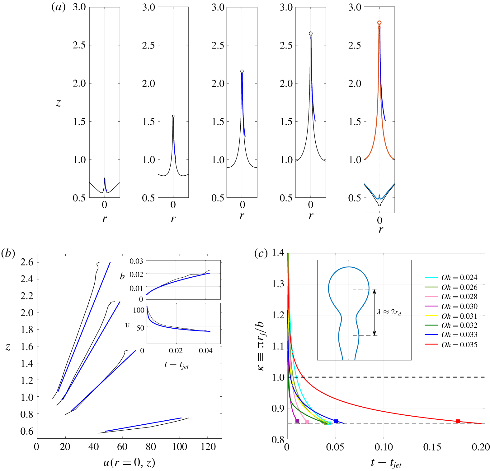
 $u(z,t)$, in a finite spatial region located upstream the drop, which suffices to correctly evaluate the mass and momentum fluxes entering the drop; see figures 3(a)–3(b). Let us point out that the very good agreement depicted in figures 3(a)–3(b) between the jet shapes calculated numerically using GERRIS and our analytical prediction in (3.7) could have been extended to a larger spatial region. This could have been done by providing correct boundary conditions to the parabolic set of (3.2) during a longer time period. However, it is not our goal here to predict the full shapes of the Worthington jets, but the diameters and the velocities of the droplets ejected. In this regard, the insets in figure 3(b) show that the time evolutions of the radius and the velocity of the tip of the jet predicted solving (3.1) and (3.7) (blue lines) closely follow the time evolutions calculated numerically using GERRIS (black lines). We checked that the good agreement shown in figure 3(a,b) between predictions and numerical results extends to the whole range of values of
 $Oh$ investigated here.
Since the theoretical model presented here is able to correctly capture the time evolutions of both  $v(t)$ and
 $b(t)$ (see the inset in figure 3b) the only missing ingredient in order to predict the drop radius and drop velocity is to determine the instant of time the jet tip breaks into drops.
(a) Time sequence showing the comparison between the spatio-temporal evolution of the jet radius and the model prediction (blue line) calculated for  $Bo=0.01$ and
 $Oh=0.024$ at the following instants of time:
 $t=0.463,\,0.476,\,0.489$ and
 $0.502$. The last frame in the sequence corresponds to the instant of time,
 $t=0.506$, the jet breaks into drops, and includes the shapes of the jet for instants of time close to its inception to stress the fact that the final drop diameter is much larger than the initial one. (b) Comparison between the spatio-temporal evolution of the jet velocity calculated numerically and that predicted by the model (blue line). The predicted values could be closer to the calculated ones if the pressure gradient term was added into the momentum equation (3.2), as is shown in the Supplementary Material. (c) The different continuous lines indicate the time evolution of the dimensionless wavenumber calculated by solving equations (3.1) using the analytical expressions in (3.7) for values of the Ohnesorge number around the one at which the minimum drop radius is attained. The breakup instants calculated using GERRIS, which are indicated using filled squares, reveal that a drop is ejected when the value of the ratio
 $\unicode[STIX]{x03C0}\,r_{j}/b$ calculated using the system (3.1) is such that
 $\unicode[STIX]{x03C0}\,r_{j}/b=0.85$.

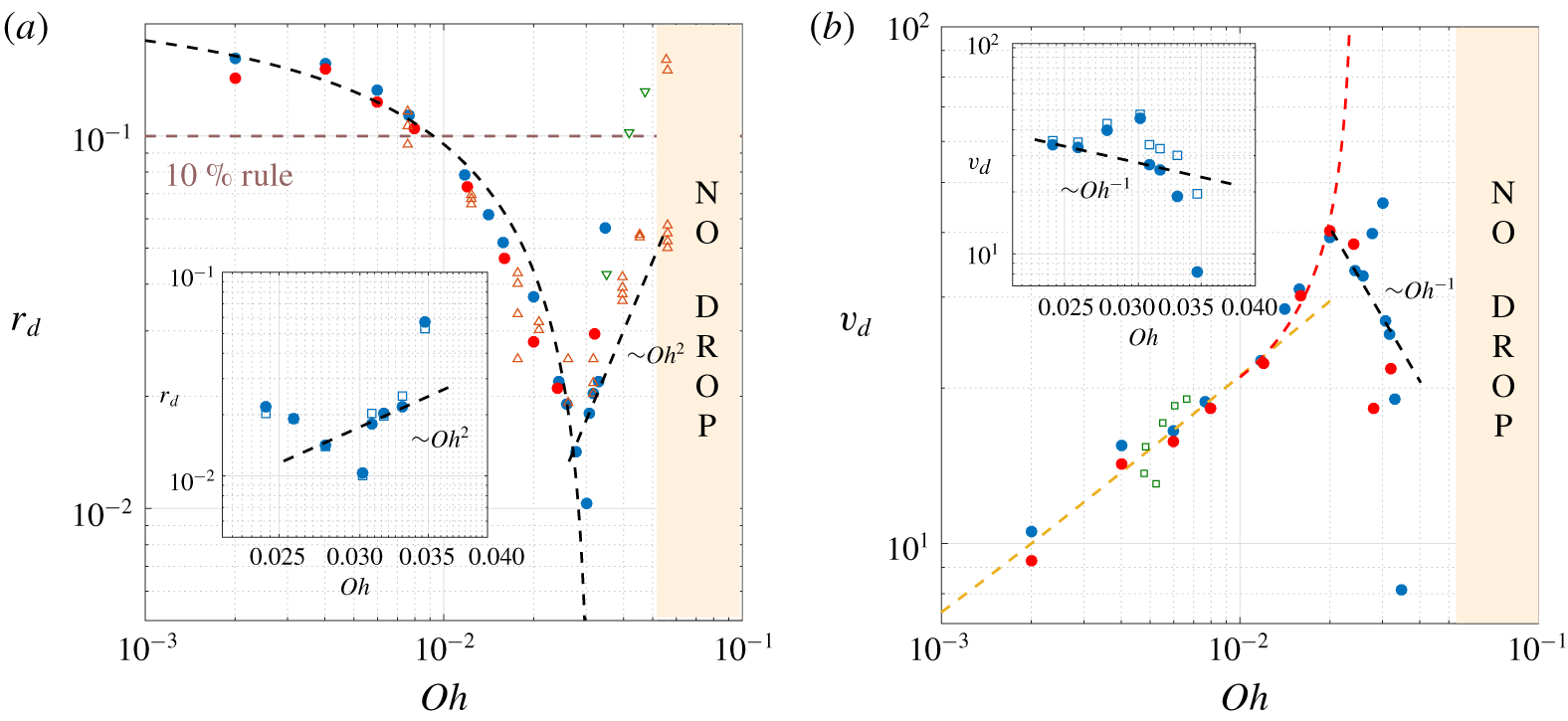
Numerical results for the radius (a) and velocity (b) of the top droplet ejected after the bursting of a bubble for  $Bo=0.01$ (solid blue dots) and
 $Bo=0.05$ (solid red dots). Panel (a) includes the experimental data reported in Brasz et al. (Reference Brasz, Bartlett, Walls, Flinn, Yu and Bird2018) (orange and green triangles) as well as the predicted values of
 $r_{d}$ calculated using either (3.9) or
 $r_{d}=18.45Oh^{2}$, finding a fair agreement between the predicted and calculated values. The minimum value of
 $r_{d}$ is reached at
 $Oh=0.03$. Panel (b) includes the droplet velocities reported in Ghabache et al. (Reference Ghabache, Antkowiak, Josserand and Séon2014) (green squares) and the predicted values of
 $v_{d}$ using either equation (3.10) or
 $v_{d}=0.784Oh^{-1}$, finding a fair agreement between the predicted and calculated values. The insets in (a,b) show the predictions of the full model with
 $\unicode[STIX]{x1D705}_{c}=0.85$ (see figure 3c) for values of the Ohnesorge number in the region where both
 $r_{d}$ and
 $v_{d}$ experience abrupt variations with
 $Oh$, finding a fair agreement between the values calculated using GERRIS (filled symbols) and the full model (open symbols); notice that both data sets mostly overlap.

3.1 Jet breakup condition
The radius and the velocity of the first droplet ejected is calculated here particularizing the functions  $b(t)$ and
 $v(t)$ (see the inset in figure 3b) at the instant the jet tip breaks as a consequence of the growth of a capillary instability. Since the wavelength of the capillary perturbation can be approximated by the diameter of the droplet, as is suggested by the inset of figure 3(c), our criterion for capillary breakup can be expressed as the instant of time for which the dimensionless wavenumber,
 $\unicode[STIX]{x1D705}=\unicode[STIX]{x03C0}r_{j}(t)/b(t)$, verifies the condition
 $\unicode[STIX]{x03C0}r_{j}/b=\unicode[STIX]{x1D705}_{c}$, with
 $\unicode[STIX]{x1D705}_{c}<1$ (Rayleigh Reference Rayleigh1878) a constant. We do not predict here the value of this free constant
 $\unicode[STIX]{x1D705}_{c}$, but fix it here by comparing the model predictions with the numerical results. Indeed, figure 3(c) represents, with continuous lines, the time evolutions of the ratio
 $\unicode[STIX]{x03C0}r_{j}(t)/b(t)$ obtained by solving the model equations (3.1) using the analytical expressions in (3.7) for several values of
 $Oh$. In each of these curves, we include a filled square corresponding to the jet breakup time calculated using GERRIS and, in all cases considered, we find that the breakup instant predicted using the GERRIS values takes place when the ratio
 $\unicode[STIX]{x03C0}r_{j}/b$ calculated using our model verifies the condition
 $\unicode[STIX]{x03C0}r_{j}/b=\unicode[STIX]{x1D705}_{c}$, with
 $\unicode[STIX]{x1D705}_{c}=0.85$. This fact confirms our hypothesis that the breakup instant can be characterized through the value of the ratio
 $\unicode[STIX]{x03C0}r_{j}/b$. Notice that the value for
 $\unicode[STIX]{x1D705}_{c}$ found here is slightly larger than the dimensionless wavenumber of fastest growth rate of capillary perturbation calculated by Rayleigh (Reference Rayleigh1878) for the case of cylindrical jets,
 $\unicode[STIX]{x1D705}_{c}\simeq 0.7$. However, this is not surprising in our case because Gordillo & Gekle (Reference Gordillo and Gekle2010) reported that the wavelengths of capillary perturbations leading to the end-pinching of stretched Worthington jets is close to the jet perimeter, which implies values of the dimensionless wavenumber of fastest growth rate larger than 0.7.
The insets in figure 4 show the comparison between the values of  $r_{d}$ and
 $v_{d}$ calculated numerically using GERRIS (full symbols) and those predicted by our model (open symbols); the latter obtained solving (3.1) and applying the jet breakup condition
 $\unicode[STIX]{x03C0}r_{j}/b=0.85$. The inset in figure 4(a) shows that most of the predicted values overlap the ones calculated using GERRIS. The good agreement between predictions and numerical results in the complex region where both
 $r_{d}$ and
 $v_{d}$ behave non-monotonically with
 $Oh$ validates our approach.
3.2 Scaling the size and velocity of the primary droplet
While the model developed in the previous sections is capable of predicting, with great accuracy, the diameters and velocities of the first drop ejected, it is of little practical use since it requires one to solve a system of ordinary differential equations. The purpose here is to derive approximate algebraic equations for both  $r_{d}$ and
 $v_{d}$, making use of our recent result in Gordillo & Rodríguez-Rodríguez (Reference Gordillo and Rodríguez-Rodríguez2019), where we derived expressions for both the radius and the velocity of the incipient jet,
 $r_{jet}$ and
 $v_{jet}$, respectively (see figure 1a), as a function of the Ohnesorge number.
The model represented by (3.1) and (3.7) and, most importantly, the breakup criterion deduced here,  $\unicode[STIX]{x03C0}r_{j}/b=0.85$, are free of parameters, with the exception of the small air drag term in (3.1) – which, in fact, we could have neglected. Since the system of differential equations only receives information of the bulk flow through the initial conditions, which depend on
 $Oh^{1/2}$ for
 $Oh<Oh_{c}$, we assume that
 $$\begin{eqnarray}r_{d}=r_{jet}+f(Oh^{1/2})\simeq r_{jet}+C_{1}+C_{2}\,Oh^{1/2}+O(Oh),\end{eqnarray}$$
where we have made use of the fact that  $Oh\ll 1$. Hence, making use of equations (2.1) and (3.8), the radius of the ejected droplet can be expressed as
 $$\begin{eqnarray}r_{d}=K_{b}(Bo)(1-(Oh/Oh_{c}^{\prime }(Bo))^{1/2}),\quad \text{if }Oh<Oh_{c}^{\prime },\end{eqnarray}$$
with  $K_{b}(Bo)$ and
 $Oh_{c}^{\prime }(Bo)>Oh_{c}(Bo)$ constants that, we found, hardly vary with
 $Bo$ for
 $Bo\leqslant 0.05$. Following the same reasoning as before, since the initial radius of the jet scales as
 $r_{jet}\propto Oh^{2}$ when a bubble is entrapped (see 2.3), it is also expected that
 $r_{d}\propto Oh^{2}$ for larger values of the Ohnesorge number.
Figure 4(a) shows that the values of  $r_{d}$ calculated using (3.9) with
 $K_{b}=0.22$,
 $Oh_{c}^{\prime }=0.031$, compare favourably with the numerically calculated ones for
 $Oh\lesssim 0.028$ and also that
 $r_{d}=18.45Oh^{2}$ approximates well the data for the small interval of values
 $0.028\leqslant Oh\leqslant 0.035$. We found, however, no simple way of predicting
 $r_{d}$ in a very short range of values around
 $Oh=0.03$ and also around
 $Oh\approx 0.04$, but the complex dependence close to these two values of
 $Oh$ is reproduced by the full model, which requires the integration of ordinary differential equations, as is shown in the inset of figure 4(a). Our numerical results in figure 4(a) also reveal that no droplets are ejected for
 $Oh\gtrsim 0.04$. Indeed, the
 $r_{d}\propto Oh^{2}$ prediction deteriorates for the larger values of
 $Oh$ because, for values of the Ohnesorge number
 $Oh\approx Oh_{d}$, the amplitude of the capillary waves excited during the rim retraction process are highly attenuated by viscosity, reducing the size of the entrapped bubble or even preventing the entrapment (see figure 2) and, as a consequence, reducing the intensity of the Worthington jet.
Let us finally point out that the numerical results depicted in figure 4(a) also show that the main influence of the Bond number on  $r_{d}$ is appreciated at the minimum radius, with
 $\min (r_{d}(Bo=0.05))\simeq 0.015$ and
 $\min (r_{d}(Bo=0.01))\simeq 0.01$.
Following the same reasoning as before, the velocity of the droplets ejected can also be expressed, for  $Oh<Oh_{c}$, as
 $v_{d}=v_{jet}+g(Oh^{1/2})\simeq v_{jet}+D_{1}+D_{2}\,Oh^{1/2}$, with
 $v_{jet}$ given in (2.2), and hence, figure 4(b) represents the functions
 $$\begin{eqnarray}\left.\begin{array}{@{}c@{}}v_{d}=1+31(Oh/Oh_{c})^{1/2},\quad \text{if }Oh<0.01,\\ v_{d}=12.5(1-(Oh/Oh_{c})^{1/2})^{-1/2},\quad \text{for }0.01\leqslant Oh<0.024\quad \text{and}\\ v_{d}=0.784Oh^{-1},\quad \text{for }Oh>0.024,\end{array}\right\}\end{eqnarray}$$
with the latter expression for  $v_{d}$ in (3.10) motivated by (2.3). Once the free constants are properly chosen, the function
 $v_{d}(Oh)$ in (3.10) agrees well with the numerical results depicted in figure 4(b), except when
 $Oh$ approximates either
 $Oh_{c}$ or
 $Oh_{d}$, for the reasons explained above. In these cases, the full model should be used to predict
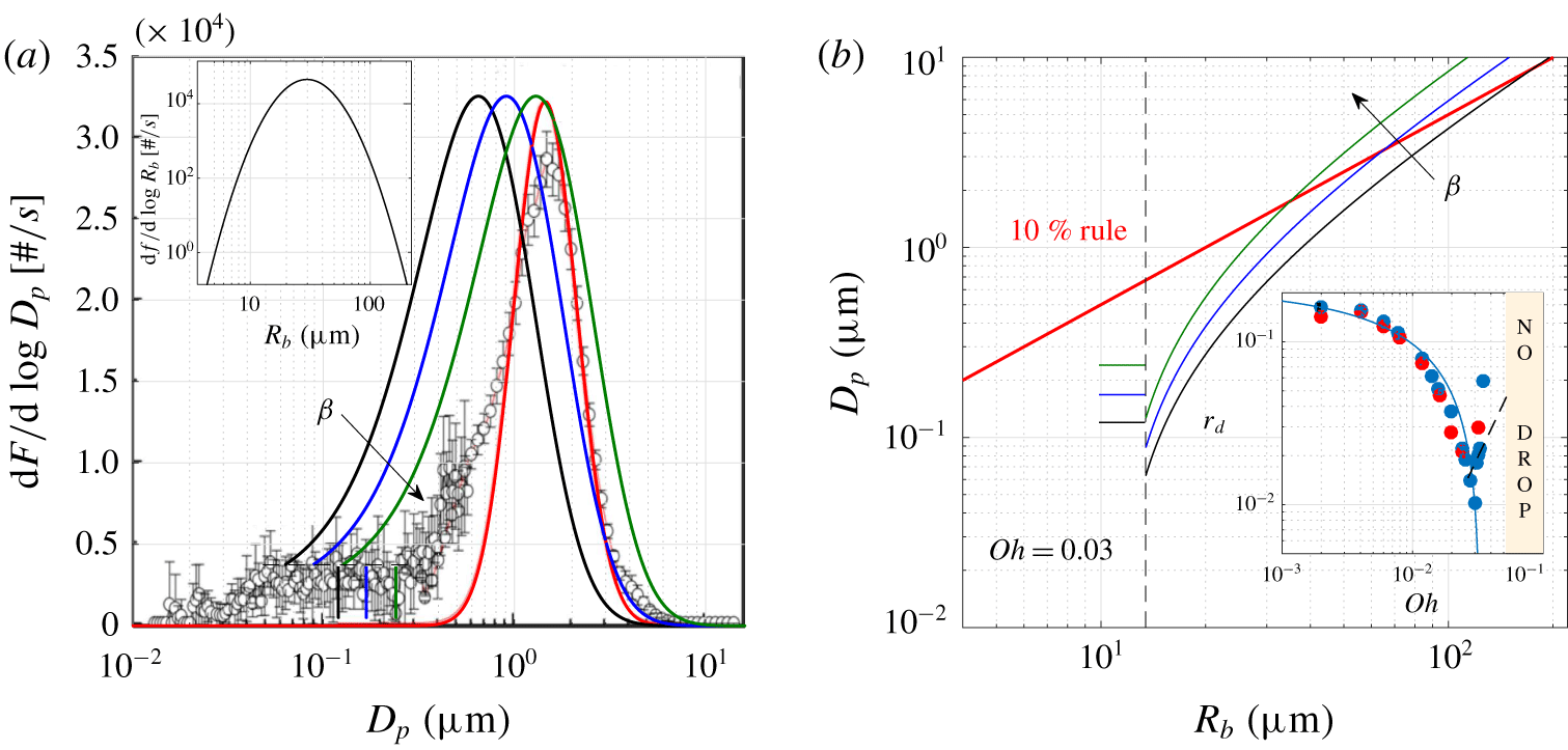
 $v_{d}$, as the inset of figure 4(b) shows. To further test the utility of our simplified description presented here, which already predicts the trend exhibited by the experimental data reported in Brasz et al. (Reference Brasz, Bartlett, Walls, Flinn, Yu and Bird2018) (see figure 4a), we have made use of the results in Wang et al. (Reference Wang, Deane, Moore, Ryder, Stokes, Beall, Collins, Santander, Burrows and Sultana2017), who, in their figure 1, provided the measured aerosol particle flux produced by a flux of bubbles with a certain size distribution (see figure 5a). Assuming that each bubble produces just one drop, using the 10 % rule for
 $r_{d}$ and approximating the dry diameter as
 $D_{p}=0.5R_{d}$, Wang et al. (Reference Wang, Deane, Moore, Ryder, Stokes, Beall, Collins, Santander, Burrows and Sultana2017) obtained the red line in figure 5(a), which compares favourably with part of the experimental data, but which does not predict the production of submicrometric particles, which play an essential role in atmospheric dynamics (Wang et al. Reference Wang, Deane, Moore, Ryder, Stokes, Beall, Collins, Santander, Burrows and Sultana2017). Figure 5(a) also includes the distribution of particles calculated assuming that just one single drop is produced per bursting bubble, taking
 $D_{p}=\unicode[STIX]{x1D6FD}R_{d}$, with
 $\unicode[STIX]{x1D6FD}$ a parameter that accounts for evaporation effects, and using the equation for
 $r_{d}$:
 $$\begin{eqnarray}\left.\begin{array}{@{}c@{}}r_{d}=0.2\left(1-\left(Oh/0.033\right)^{1/2}\right),\quad \text{if }Oh\leqslant 0.03\quad \text{and}\\ r_{d}=18.45\,Oh^{2},\quad \text{for }0.03<Oh\leqslant 0.035,\end{array}\right\}\end{eqnarray}$$
which also approximates very well the numerical data (see the inset in figure 5b). In Wang et al. (Reference Wang, Deane, Moore, Ryder, Stokes, Beall, Collins, Santander, Burrows and Sultana2017) and references therein, it is assumed that  $\unicode[STIX]{x1D6FD}=0.5$; namely, that the radius of the solid particle is just one-half the original radius. But we have not found a clear justification for this particular value of
 $\unicode[STIX]{x1D6FD}$ and have chosen to vary this parameter between
 $\unicode[STIX]{x1D6FD}=0.5$ and
 $\unicode[STIX]{x1D6FD}=1$ – the latter value meaning that, after evaporation, the radius of the solid particle coincides with the initial drop radius.
(a) (Adapted from figure 1 in Wang et al. Reference Wang, Deane, Moore, Ryder, Stokes, Beall, Collins, Santander, Burrows and Sultana2017): Comparison between the predicted and measured particle diameters composing the aerosol with  $D_{p}=\unicode[STIX]{x1D6FD}\,R_{b}\,r_{d}$ and
 $\unicode[STIX]{x1D6FD}=0.5$ (black), 0.7 (blue) and 1 (green), see also panel (b). The inset represents a log-normal fit to the experimental data in Wang et al. (Reference Wang, Deane, Moore, Ryder, Stokes, Beall, Collins, Santander, Burrows and Sultana2017). (b) Particle diameters calculated as
 $D_{p}=\unicode[STIX]{x1D6FD}\,R_{b}\,r_{d}$, with
 $r_{d}$ given in (3.11). Seawater physical properties taken from Nayar et al. (Reference Nayar, Sharqawy, Banchik and Lienhard V2016) for a temperature of
 $25\,^{\circ }\text{C}$ and a salinity of
 $30~\text{g}~\text{kg}^{-1}$. Here
 $\#$ indicates number of particles or bubbles and
 $f$ or
 $F$ indicate the bubble or particle size distribution.

The shape of the distribution of diameters obtained using our results is quite similar to the experimental one and, although slightly shifted to the left, it predicts the generation of submicron-sized particles with diameters  $D_{p}<100~\text{nm}$. In any case, the differences between the predicted and measured values can be attributed to the number of simplifying hypotheses done in the calculation of
 $D_{p}$: indeed, the bubble coalescence events at the interface, which would displace the original bubble size distribution to the right, are not considered here. Also, the use of (3.11) rests on the assumption that the collapse is axisymmetric and that the interface is not rigidized by surfactants or solid particles. While it is clear that the presence of small particles or surfactants will affect the jet ejection and breakup processes, the axisymmetry hypothesis is also easily violated under realistic conditions because collective effects and the influence of neighbouring bubbles will produce an inclined jet. This is so because geometrical asymmetries cause the capillary waves travelling along the spherical surface to not reach the bottom of the cavity at the same time, distorting the base of the truncated cone from which the jet is issued.
4 Concluding remarks
With the purpose of providing closed expressions for the radius,  $r_{d}$, and velocity,
 $v_{d}$, of the first drops ejected from the tip of the fast and thin vertical jet produced at the base of the cavity of a bursting bubble, here we have extended the recent results in Gordillo & Rodríguez-Rodríguez (Reference Gordillo and Rodríguez-Rodríguez2019) by developing a one-dimensional model to describe the spatio-temporal evolution of the jet. This model, which is coupled with balances of mass and momentum at the jet tip, reproduces very well the spatio-temporal evolution of the radius of the jet, of the jet velocity field and the time variations of the thickness,
 $b(t)$, and velocity,
 $v(t)$, of the tip of the jet. The particularization of
 $b(t)$ and
 $v(t)$ at the instant of time the dimensionless wavenumber is such that capillary waves grow and break the jet, provides the values of
 $r_{d}$ and
 $v_{d}$ as a function of the Ohnesorge number,
 $Oh$. Since this method requires the integration of a system of equations, it is not of practical use in realistic applications. Hence, we have deduced simple algebraic equations for
 $r_{d}$ and
 $v_{d}$, which are in fair agreement with our own numerical results. The equations for
 $r_{d}$ and
 $v_{d}$ are expressed, for
 $Oh\lesssim 0.03$, in terms of
 $Oh^{1/2}$, with
 $Oh^{1/2}$ proportional to the dimensionless wavelength of the capillary wave which triggers the jet ejection process from the base of a truncated cone. However, for larger values of the Ohnesorge number, the entrapment of a bubble below the jet causes viscosity to limit the maximum attainable velocity and the minimum jet radius – a fact explaining that, for
 $0.025\lesssim Oh\lesssim 0.035$, the radii and velocities of the droplets ejected experience an abrupt change of trend in a narrow range of values of
 $Oh$, with the scales in this region given by
 $r_{d}\propto Oh^{2}$ and
 $v_{d}\propto Oh^{-1}$. The equation for
 $r_{d}$ deduced here has been applied to predict the diameters of the submicrometric aerosol particles produced by the bubble size distribution reported in Wang et al. (Reference Wang, Deane, Moore, Ryder, Stokes, Beall, Collins, Santander, Burrows and Sultana2017) and our results are similar to the flux of submicron-sized particles measured experimentally – a fact indicating that our findings could be used to improve the aspects of climate models related with the production of sea spray aerosol particles, which play an essential role absorbing and scattering radiation and as ice and cloud condensation nuclei.
Acknowledgements
This work has been supported by the Spanish MINECO under Project DPI2017-88201-C3-1-R, partly financed through European funds. F.J.B.R. acknowledges funding received from the Spanish Government through grant IJCI 2016-30126. The authors are grateful to J. Rodríguez-Rodríguez for sharing with us his codes and for very useful suggestions.
Declaration of interests
The authors report no conflict of interest.
Supplementary material
Supplementary material is available at https://doi.org/10.1017/jfm.2019.1061.