1 Introduction
Solitary waves have been used in the literature to study the characteristics and behaviour of weakly nonlinear localized long waves. Extensive attention has been given to the run-up of solitary waves on sloping beaches (e.g. Goring Reference Goring1978; Pedersen & Gjevik Reference Pedersen and Gjevik1983; Kobayashi, Otta & Roy Reference Kobayashi, Otta and Roy1987; Synolakis Reference Synolakis1987; Kobayashi, DeSilva & Watson Reference Kobayashi, DeSilva and Watson1989; Lin, Chang & Liu Reference Lin, Chang and Liu1999; Carrier, Wu & Yeh Reference Carrier, Wu and Yeh2003; Li & Raichlen Reference Li and Raichlen2003; Hsiao et al. Reference Hsiao, Hsu, Lin and Chang2008; Knowles & Yeh Reference Knowles and Yeh2018), fission and breaking from wave propagation over submerged steps (e.g. Losada, Vidal & Medina Reference Losada, Vidal and Medina1989; Yasuda, Mutsuda & Mizutani Reference Yasuda, Mutsuda and Mizutani1997; Liu & Cheng Reference Liu and Cheng2001) and vortex evolution and advection around a submerged obstacle (e.g. Chang, Hsu & Liu Reference Chang, Hsu and Liu2001; Huang & Dong Reference Huang and Dong2001; Lin et al. Reference Lin, Chang, Ho and Chang2006; Lin & Huang Reference Lin and Huang2010). In addition, performance of a submerged breakwater has been investigated extensively using solitary waves (e.g. Mei & Black Reference Mei and Black1969; Massel Reference Massel1983; Seabra-Santos, Renouard & Temperville Reference Seabra-Santos, Renouard and Temperville1987; Grue Reference Grue1992; Rey, Belzons & Guazzelli Reference Rey, Belzons and Guazzelli1992; Ting & Kim Reference Ting and Kim1994; Zhuang & Lee Reference Zhuang and Lee1997; Tang & Chang Reference Tang and Chang1998; Huang & Dong Reference Huang and Dong1999; Chang et al. Reference Chang, Hsu and Liu2001; Chang, Hsu & Liu Reference Chang, Hsu and Liu2005).
Solitary-wave interaction with a submerged sill has received some attention in the literature. Here we use the term ‘sill’ to represent a straight and uniform underwater ridge that divides a water body of uniform depth. The characterization of the wave–sill interaction has been focused on reflection and transmission coefficients (Lin Reference Lin2004). Studies involving monochromatic waves have identified that the height of the sill is important for determining these coefficients (e.g. Losada, Silva & Losada Reference Losada, Silva and Losada1996; Christou, Swan & Gudmestad Reference Christou, Swan and Gudmestad2008; Young & Testik Reference Young and Testik2011). Analytical studies on solitary wave interaction with a submerged sill has been limited (Lin Reference Lin2004; Lin & Liu Reference Lin and Liu2005). Instead, most studies that characterize wave–sill interaction have been primarily numerical and experimental.
Seabra-Santos et al. (Reference Seabra-Santos, Renouard and Temperville1987) examined the motion of solitary waves over a submerged triangular-shaped sill. Their study predicts reflection and the formation of a perturbed transmitted wave with a trailing, small-amplitude dispersive wavetrain. Cooker et al. (Reference Cooker, Peregrine, Vidal and Dold1990) extended this work by studying solitary-wave interaction with a submerged semicircular sill, using an extension of the numerical model by Dold & Peregrine (Reference Dold and Peregrine1986). Results from Cooker et al. (Reference Cooker, Peregrine, Vidal and Dold1990) found a variety of different interactions that depend on the wave height and semicircular-sill size. Four types of interactions were described: small dispersive wavetrain development behind the transmitted wave, crest–crest exchange, forwards breaker and backwards breaker. These results were confirmed by a limited number of experiments, although the backwards breaker was not observed in the laboratory. Grilli, Losada & Martin (Reference Grilli, Losada and Martin1994) expanded this work to trapezoidal-shaped obstacles (a model of a submerged breakwater) and characterized wave behaviour as a function of the obstacle and incident wave height. Their laboratory observations found that the waves may break forwards or backwards downstream of the obstacle.
In the present study, we expand the experimental work of Seabra-Santos et al. (Reference Seabra-Santos, Renouard and Temperville1987), Cooker et al. (Reference Cooker, Peregrine, Vidal and Dold1990) and Grilli et al. (Reference Grilli, Losada and Martin1994) to study the effect of sill’s breadth on the transmitted solitary waves. Here we use a rectangular-shaped flat plate for the sill. We focus on the transformation of the solitary wave at a significant distance after interaction with the sill, as well as the characterization of wave behaviour over the sill. It is noted that, in a companion paper (Part 2, Yeh et al. Reference Yeh, Ko, Knowles and Harry2019), we study the effect of a submerged sill placed along the direction of wave propagation; in other words, the uniform disturbance is applied to a finite breadth continually along the propagation.
2 Laboratory experiments
2.1 Experimental set-up
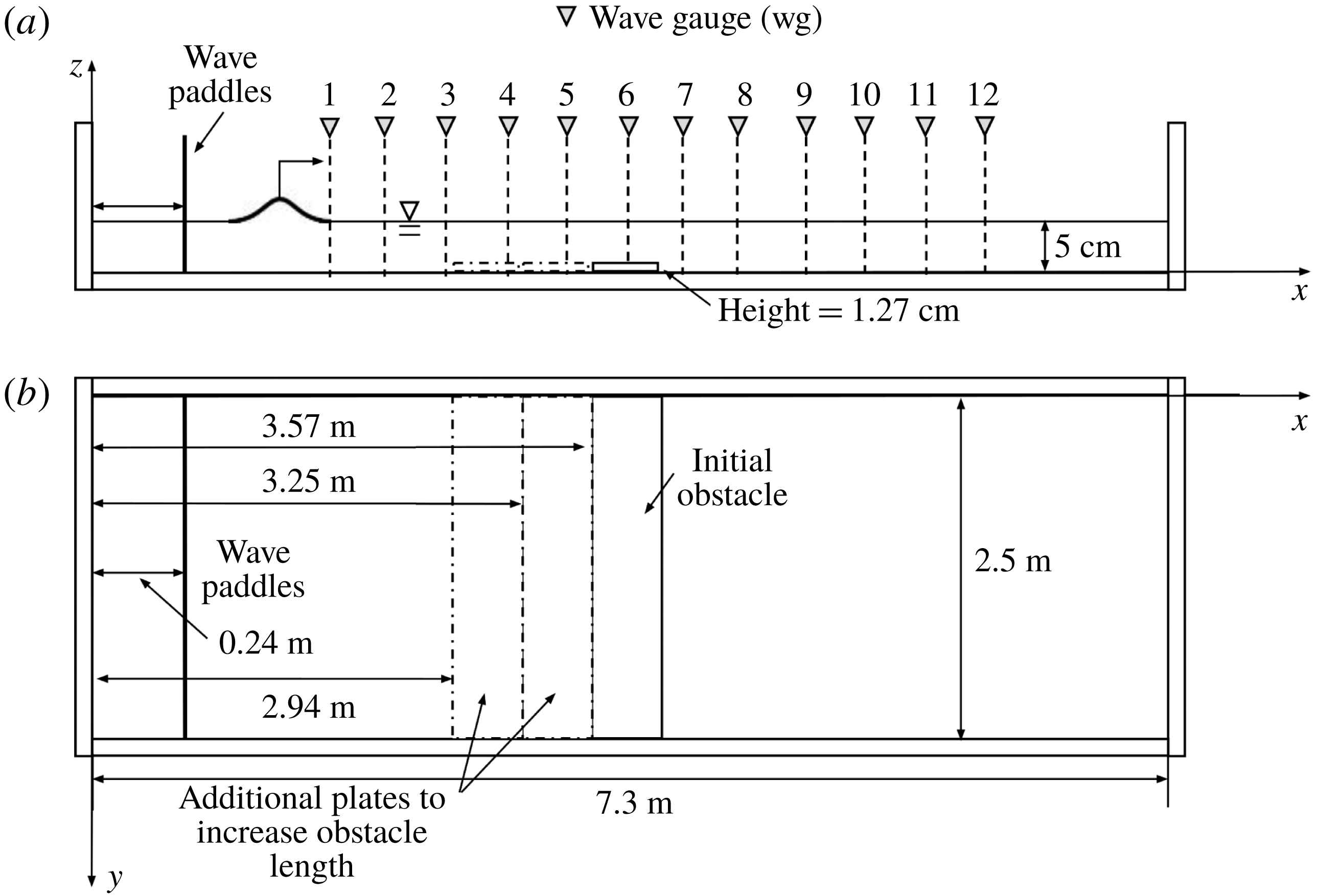
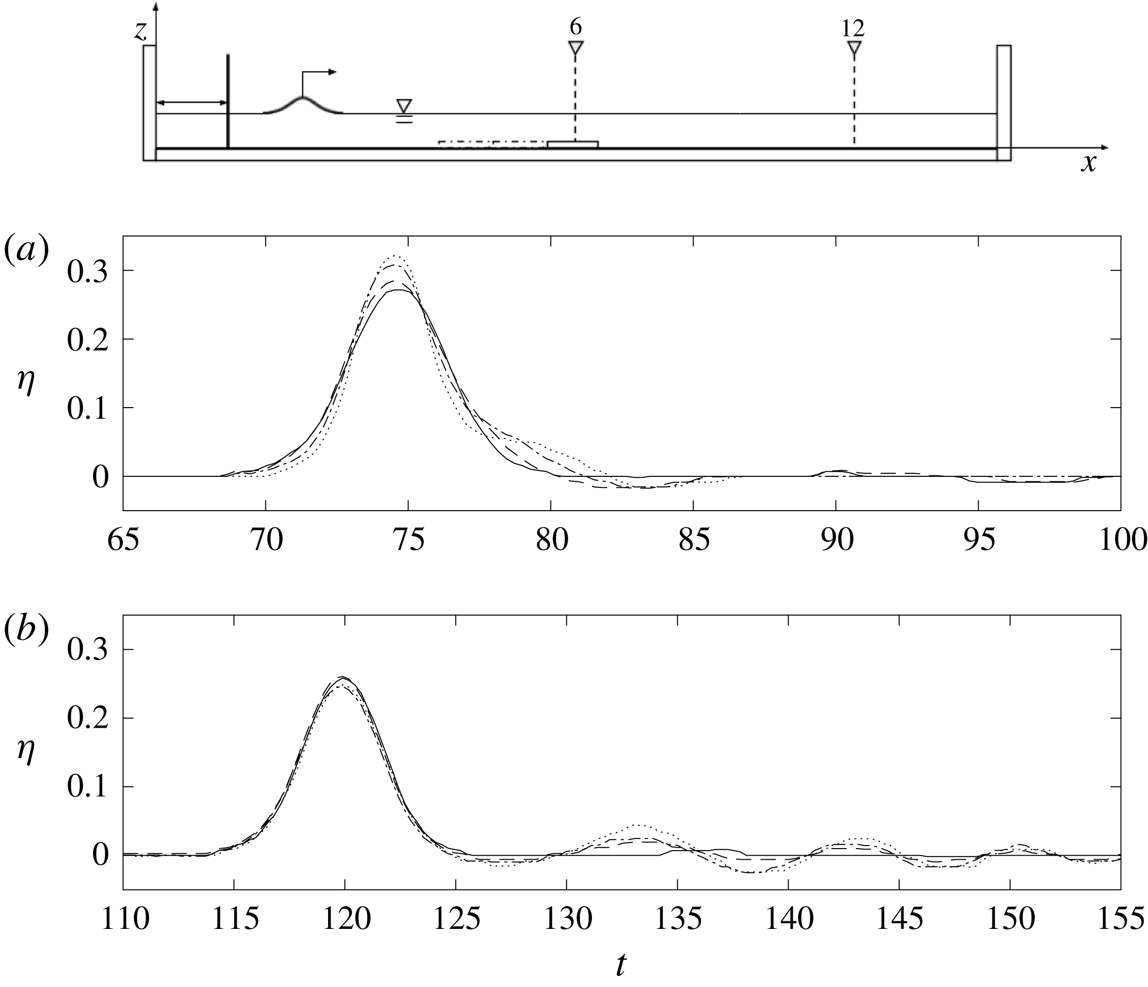
Experiments are performed in a wave tank with a submerged rectangular-shaped sill spanning the width of the tank: see figure 1. The wave tank, 7.3 m long, 2.5 m wide and 0.30 m deep, is elevated 1.2 m above the laboratory floor. The bottom and side walls of the tank are made of 12.7 mm thick glass plates. This design facilitates the use of optical techniques to measure wave fields. As discussed later, the glass bottom eliminates laser-sheet reflection; such reflection can cause substantial noise in wave-profile measurements from the laser-induced fluorescence (LIF) technique. The tank bed was levelled to form the horizontal plane with a tolerance of
 $\pm 0.8~\text{mm}$
. This degree of precision is important for the study of nonlinear ‘long’ waves. The wave tank is relatively wide in comparison with the water depth – the quiescent water depth is set at
 $h_{0}=5.0$
cm in this study – so that any disturbance that may be created along the side walls should be negligible.
Schematic drawings of the wave tank: (a) elevation view showing the position of wave gauge measurements; (b) plan view showing the position of three different submerged sill breadths. To fit the glass plate, the tank breadth is narrowed by placing a vertical rigid waveguide (one of the side walls shown in (b) is the waveguide). The coordinate system defined in the figure is used to describe positioning within the wave tank.

The wave basin is equipped with a wavemaker along the 2.5 m long head wall, capable of generating arbitrarily shaped waves. The wave paddles are pushed by linear motors, which are inherently more accurate for producing linear positioning than traditional rotary motors. The maximum horizontal stroke for the wave paddles is 55 cm – adequate for the generation of long waves in the water depth of
 $h_{0}=5.0~\text{cm}$
. (In the present experiments, the maximum stroke used was 9.0 cm.) The generated waves are repeatable: Li, Yeh & Kodama (Reference Li, Yeh and Kodama2011), who performed their experiments using the same apparatus, reported that the maximum error for a solitary wave was less than 0.1 % of the depth when the wave amplitude was 1.73 cm in water depth
 $h_{0}=6.0~\text{cm}$
.
Figure 1 shows a schematic sketch of the experimental set-up with the submerged sill placed in the transverse orientation. Glass plates are used to create the sill. Each glass plate has dimensions of 0.3175 m in width and 0.0127 m in height, and spans 2.5 m from side wall to side wall. The plate is placed directly on the tank bottom oriented such that the 2.5 m dimension is perpendicular to the direction of wave propagation. Three glass plates are used to create sills of different breadths (0.3175 m, 0.6350 m, 0.9525 m). The initial glass plate is placed with its upstream edge at 3.57 m from the wave tank head wall. The subsequent glass plates, for changing the sill breadth, are placed on the upstream side of the initial sill to maximize the post-sill propagation distance in the wave tank. It is noted we add a rigid vertical waveguide along the tank to match the sill (comprised of glass plates) dimensions with the width of the tank.
2.2 Wave generation and measurements
To generate clean solitary waves, we use the higher-order solution by Grimshaw (Reference Grimshaw1971), which is presented explicitly by Tanaka (Reference Tanaka1993). In non-dimensionalized form with the use of the ambient water depth
 $h_{0}$
for the length scale and
 $t_{0}=\sqrt{h_{0}/g}$
for the time scale (
 $g$
is the gravitational acceleration), the water-surface elevation
 $\unicode[STIX]{x1D702}$
of the higher-order solitary wave can be expressed as
 $$\begin{eqnarray}\displaystyle & \displaystyle \unicode[STIX]{x1D702}=as^{2}-{\textstyle \frac{3}{4}}a^{2}(s^{2}-s^{4})+a^{3}\left({\textstyle \frac{5}{8}}s^{2}-{\textstyle \frac{151}{80}}s^{4}+{\textstyle \frac{101}{80}}s^{6}\right), & \displaystyle\end{eqnarray}$$
where
 $a$
is the normalized wave amplitude,
 $s\equiv \text{sech}(\unicode[STIX]{x1D6FC}(x-Ft))$
,
 $F=1+\frac{1}{2}a-\frac{3}{20}a^{2}+\frac{3}{56}a^{3}$
,
 $\unicode[STIX]{x1D6FC}=\sqrt{\frac{3}{4}a}(1-\frac{5}{8}a+\frac{71}{128}a^{2})$
,
 $t$
is the normalized time and
 $x$
points in the propagation direction. With
 $\unicode[STIX]{x1D702}$
obtained from (2.1), we first compute the depth-averaged fluid velocity by
 $\bar{u}=F\unicode[STIX]{x1D702}/(1+\unicode[STIX]{x1D702})$
, then find the wave-paddle displacement,
 $x$
, by integrating
 $\text{d}x/\text{d}t=\bar{u}(x,t)$
.
Water-surface measurements are made using four ultrasonic wave gauges (General Acoustics, Model HF54 Controller and USS 02-HF Sensors). The wave gauge system uses non-intrusive devices that avoid the uncertainty of meniscus effects inherent to standard intrusive wave gauges (e.g. capacitance and resistance types gauges). This wave gauge system operates at a sampling rate of 50 Hz and has a resolution of 0.18 mm. As shown in figure 1, wave gauge measurements are taken at twelve locations for each experimental run. Since only four wave gauges are available, experiments for each condition are repeated three times. The wave gauges are attached to movable carriages and traversed from location to location in between repeated runs. It is emphasized that this laboratory apparatus together with the wavemaker system is capable of generating a precisely repeatable wave.
The LIF technique is implemented to capture the detailed wave breaking processes. The LIF technique has been used to optically record the temporal variation of the air–water interface of long waves (Yeh & Ghazali Reference Yeh and Ghazali1987; Ramsden & Raichlen Reference Ramsden and Raichlen1990; Duncan et al.
Reference Duncan, Philomin, Behres and Kimmel1994, Reference Duncan, Qiao, Philomin and Wenz1999; Gardarsson & Yeh Reference Gardarsson and Yeh2007; Diorio, Liu & Duncan Reference Diorio, Liu and Duncan2009). In the present study, the LIF method comprises of a 5 W diode-pumped solid-state laser, cylindrical lens and two front-face mirrors. The laser beam is converted to the laser sheet by the cylindrical lens, and then the laser sheet is directed to the desirable direction and location with the use of two front-face mirrors. A thin laser sheet illuminates the dyed water from above, then the dissolved fluorescein in the illuminated plane is activated and becomes fluorescent. The water surface along the illuminated line is captured with a video camera (
 $1696\times 1710~\text{pixels}$
). The captured images are rectified and processed so that the resulting images are analysed quantitatively. This technique accurately obtains temporal and spatial variations of the water surface in a non-intrusive manner at a frequency of 100 Hz.
One of the difficulties associated with the LIF technique arises from its application to images associated with a very large (or small) aspect ratio: capturing long waves with the LIF technique is not straightforward because of its inherently small vertical-to-horizontal length scale ratio. This results in insufficient resolution in the vertical direction. To circumvent this difficulty, we repeat LIF water-surface profiles on approximately 27 cm segments, and make a montage of the multiple-segment profiles to cover a sufficient span of the wave evolution. This procedure is only possible with a laboratory apparatus that is capable of precise replication. The same procedure was used previously in this laboratory for the measurements of Mach reflection by Li et al. (Reference Li, Yeh and Kodama2011) and solitary-wave collisions by Chen & Yeh (Reference Chen and Yeh2014).
2.3 Experimental conditions
The water depth for the experiments is maintained at
 $h_{0}=5.0~\text{cm}$
. From hereinafter, the parameters with the subscript ‘0’ represent the dimensional quantities. At this water depth, six different solitary-wave conditions are generated with amplitudes of
 $a_{i}(=a_{0}/h_{0})=0.1$
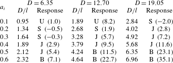
, 0.2, 0.3, 0.4, 0.5 and 0.6. For three sill breadths, there are a total of 18 conditions which are shown in table 1. In the table,
 $D=(D_{0}/h_{0})$
is the breadth of the submerged sill, and
 $D/l$
is the relative length scale of the submerged disturbance to the length of solitary wave, in which the effective wavelength,
 $l=(l_{0}/h_{0})$
, is taken as the distance for which 95 % of the volume is contained (Dean & Dalrymple Reference Dean and Dalrymple1991) and is given by
 $$\begin{eqnarray}\displaystyle & \displaystyle l=\frac{2.12}{\sqrt{a}}. & \displaystyle\end{eqnarray}$$
Because the quiescent water depth
 $h_{0}$
is fixed at 5.0 cm, the height of the sill is also fixed:
 $b=(b_{0}/h_{0})=0.254$
for all the cases studied here. In addition to the cases represented in table 1, unobstructed cases were observed by measuring the solitary-wave amplitude decay rate in the wave tank for each
 $a_{i}$
used in these experiments.
Experimental cases:
 $a_{i}$
is the amplitude of the solitary wave;
 $l$
is the effective length of the solitary wave based on (2.2);
 $D$
refers to the breadth of the sill. Wave response is expressed as: U for ‘unperturbed’, S for ‘small perturbation’, J for ‘large perturbation’ and B for ‘wave breaking. The numbers in parenthesis are the per cent (%) loss in the total mechanical energy in comparison with the corresponding unobstructed solitary wave. Any negative value in energy loss is non-physical and must be the result of insufficient wave gauge resolution for the cases of small-amplitude waves. Details of the different responses and energy losses will be discussed in § 3 and also presented graphically in figure 10.

3 Results
As mentioned, prior to examining solitary waves disturbed by the submerged sills, we first measure the ‘unobstructed’ wave amplitude decay in the wave tank (with no sill in the tank). The amplitude attenuation rate of solitary waves can be estimated theoretically based on energy dissipation in the thin laminar boundary layer on the bed (Keulegan Reference Keulegan1948), and it is written in the non-dimensionalized form
 $$\begin{eqnarray}\displaystyle & \displaystyle a^{-1/4}-a_{i}^{-1/4}=Kx, & \displaystyle\end{eqnarray}$$
where the coefficient of damping
 $K$
is
 $$\begin{eqnarray}\displaystyle & \displaystyle K=\frac{1}{12}\sqrt{\frac{\unicode[STIX]{x1D708}}{g^{1/2}h_{0}^{3/2}}}, & \displaystyle\end{eqnarray}$$
for a very wide channel, and
 $\unicode[STIX]{x1D708}$
is the kinematic viscosity of water. Note that Keulegan’s original (Reference Keulegan1948) analysis includes the effect of tank side walls. In the present experiments, the tank is very wide: the ratio of the depth to the tank breadth is
 $h_{0}/B=1/50$
. Hence the energy dissipation caused by the side walls is neglected. In (3.1) and (3.2),
 $a$
is the wave amplitude after travelling distance
 $x$
, and
 $a_{i}$
is the initial wave amplitude.
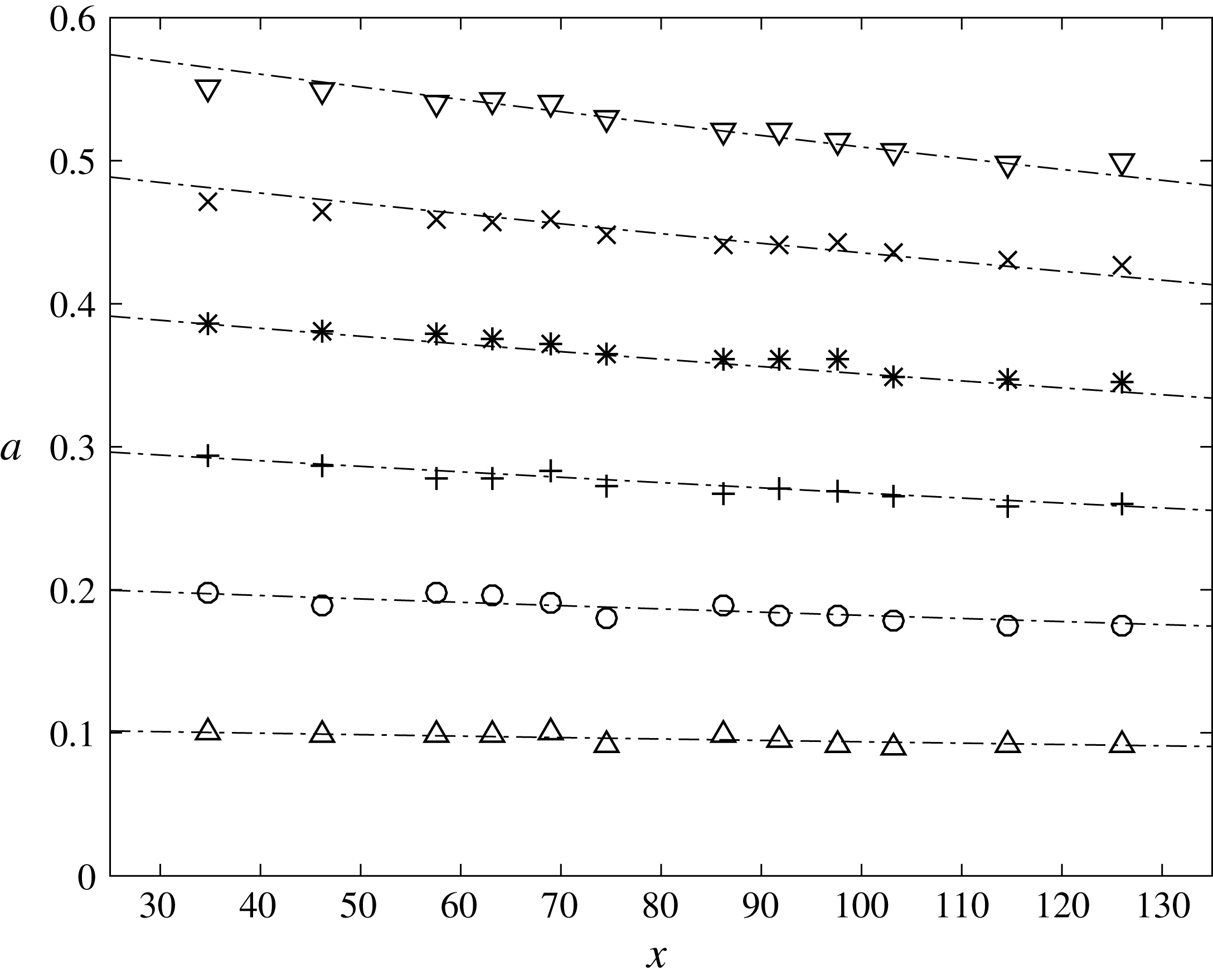
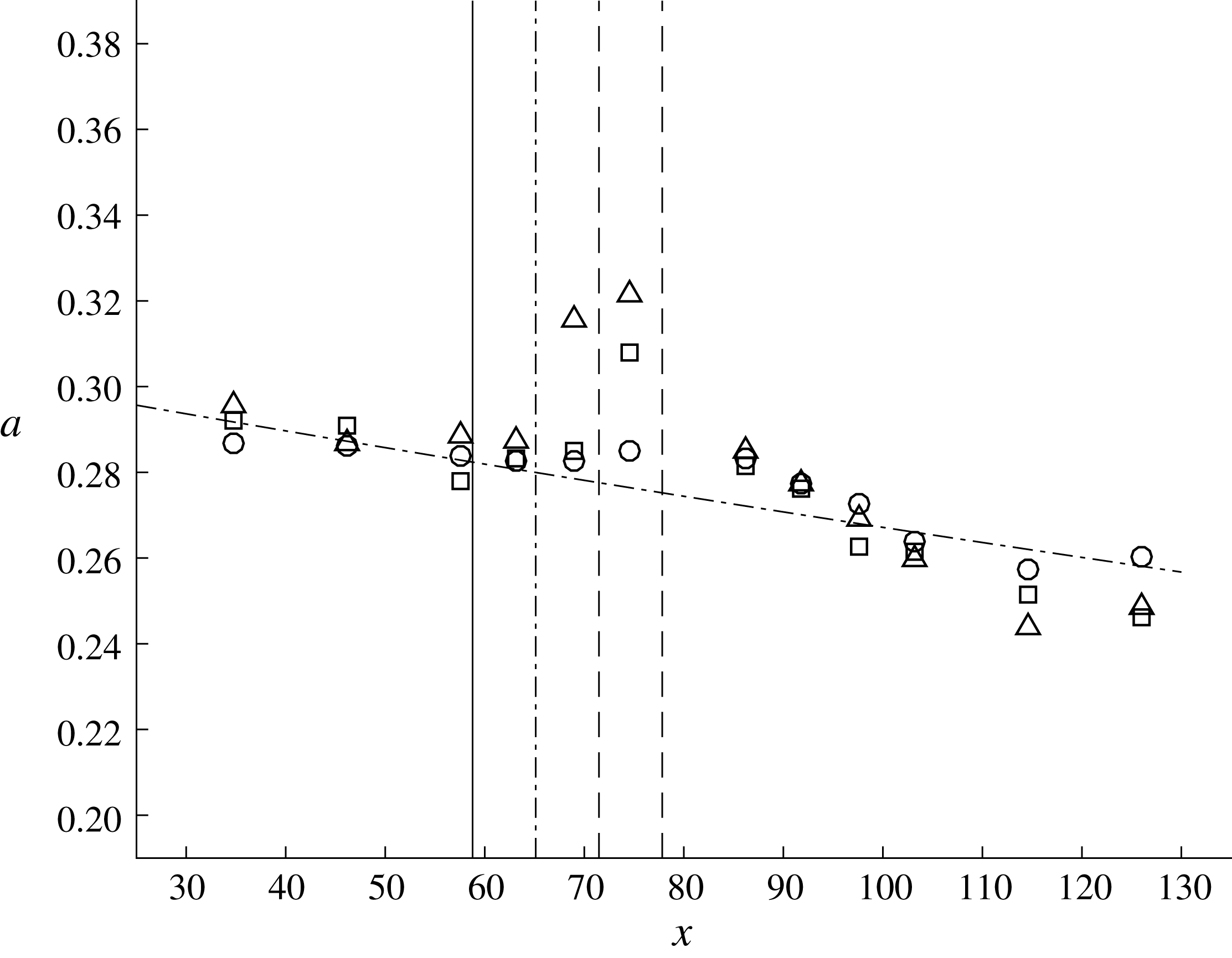
Figure 2 exhibits the comparison of the measured amplitude attenuation with the prediction made by (3.1). The agreement is excellent even for the highly nonlinear cases. The excellent agreement must be due partly to the use of very wide wave tank; hence complex energy dissipation in the side wall boundary layer, and perhaps more important, the effect of energy exchange through the confluence of the side wall and water surface is negligible in comparison with the energy dissipation in the bed boundary layer. According to Miles (Reference Miles1967) and Mei & Liu (Reference Mei and Liu1973), the small region of the water surface near the side wall plays an important role in feeding wave energy into the side wall boundary layer, which leads to energy dissipation.
Attenuation of unobstructed solitary-wave amplitudes: ▵,
 $a_{i}=0.1$
; ○,
 $a_{i}=0.2$
;
 $+,a_{i}=0.3$
; *,
 $a_{i}=0.4$
;
 $\times$
,
 $a_{i}=0.5$
; ▿,
 $a_{i}=0.6$
; – ⋅ – ⋅ –, prediction by (3.1).

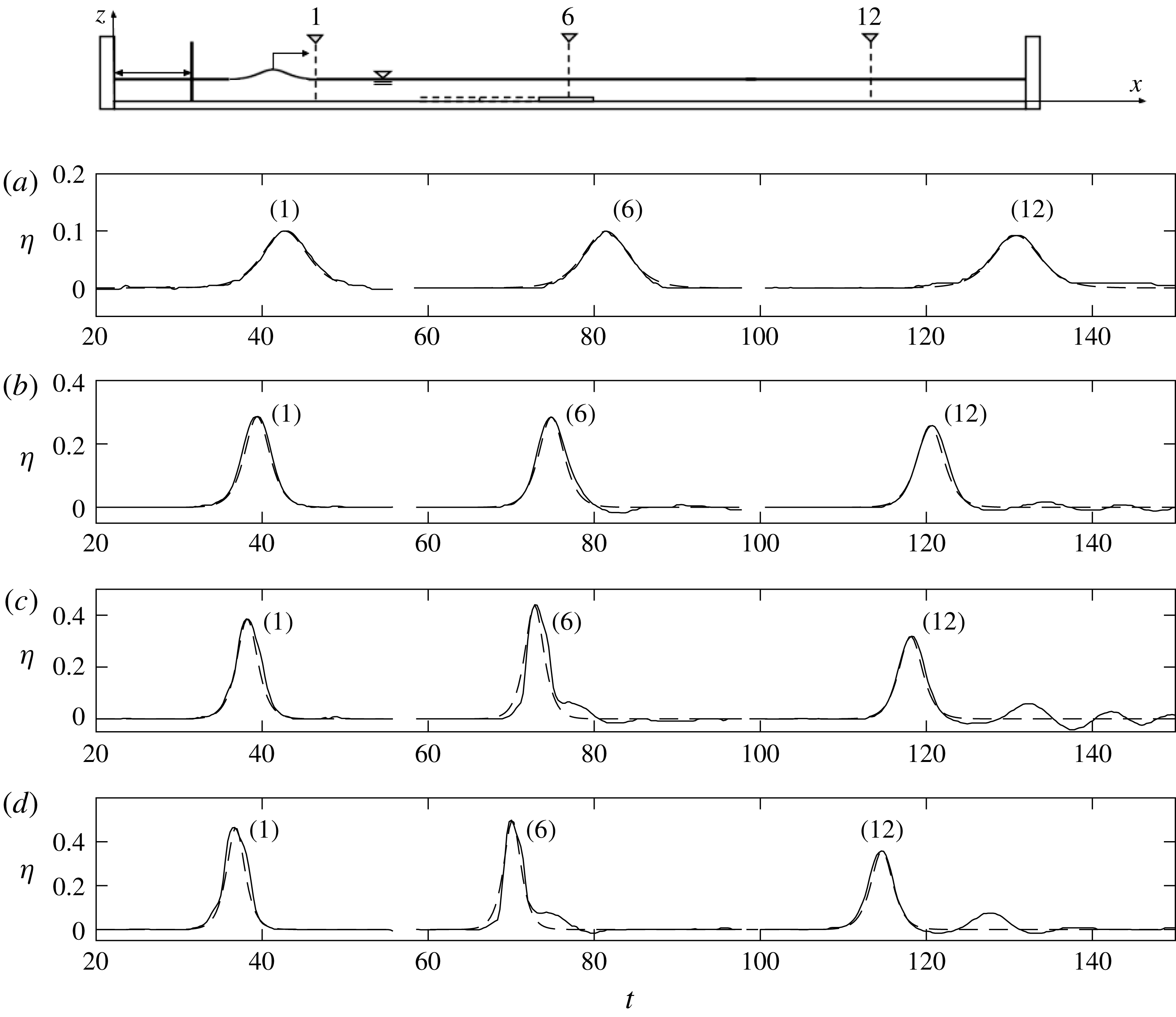
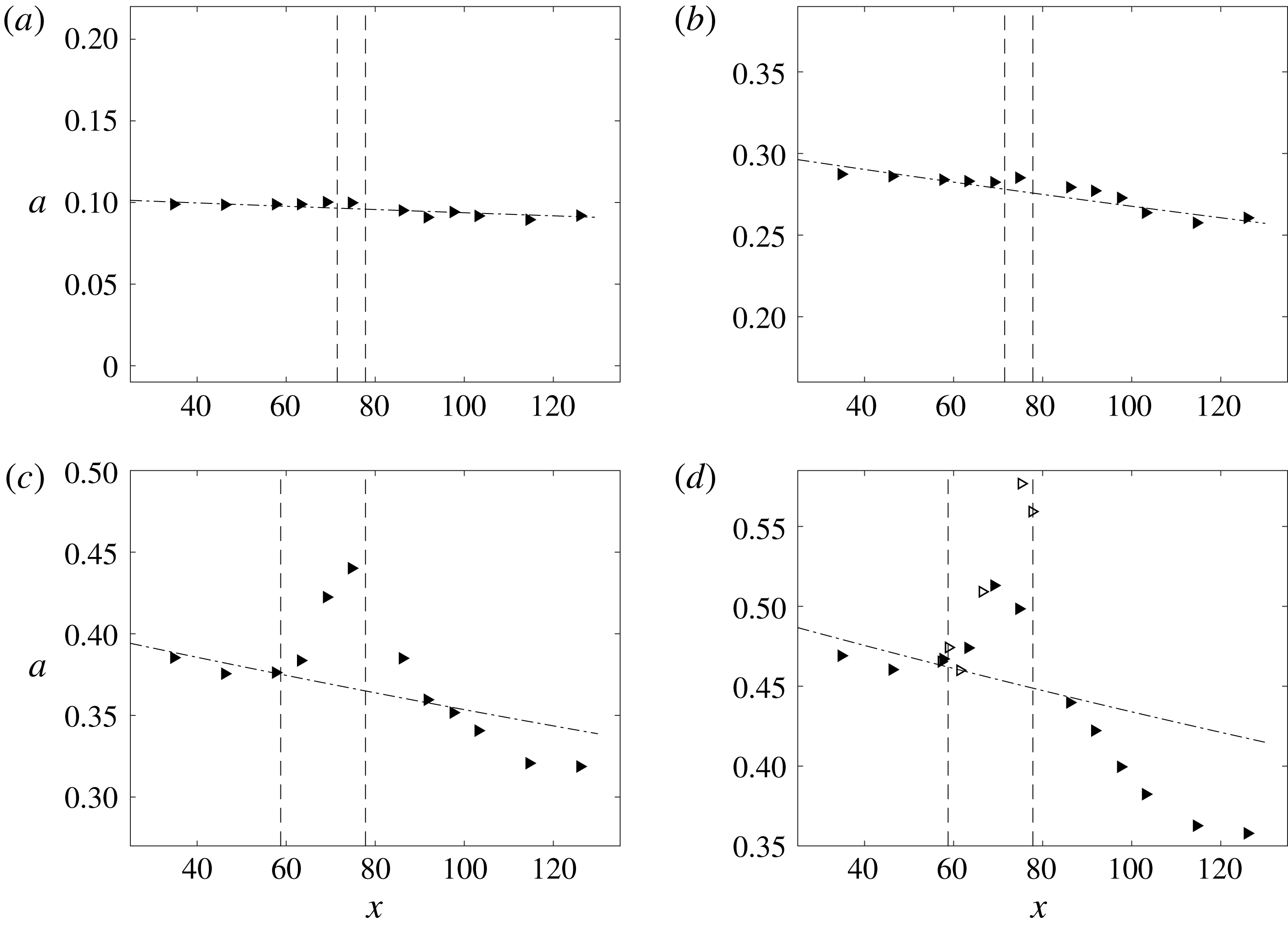
As presented in table 1, solitary-wave evolution through the disturbance of the submerged sill is categorized by four classes: (i) unperturbed, (ii) small perturbation, (iii) large perturbation and (iv) wave breaking. Figure 3 exhibits the transformation of wave profiles for those four classes. We present the representative cases for each class, namely (a) (
 $a_{i}=0.1$
,
 $D/l=0.947$
) for unperturbed; (b) (
 $a_{i}=0.3$
,
 $D/l=1.64$
) for small perturbation; (c) (
 $a_{i}=0.4$
,
 $D/l=5.68$
) for large perturbation; (d) (
 $a_{i}=0.5$
,
 $D/l=6.35$
) for wave breaking. In addition, in figure 4, we present the evolution of the amplitudes for those four cases.
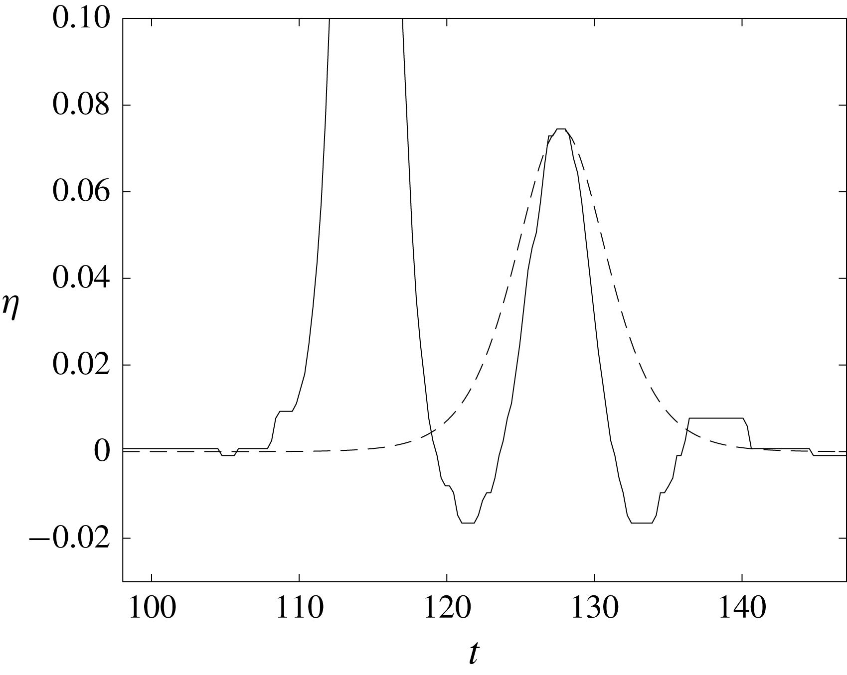
Time variation of the water-surface profile at
 $x=34.8$
(at the gauge location (1) as indicated in figure 1: close to the wave paddle),
 $x=74.7$
(at the gauge location (6) above downstream end of the sill) and
 $x=126.0$
(at the gauge location (12) near the end of the tank): (a) for the wave
 $a_{i}=0.1$
passing over a submerged sill of breadth
 $D/l=0.947$
; (b)
 $a_{i}=0.3$
,
 $D/l=1.64$
; (c)
 $a_{i}=0.4$
,
 $D/l=5.68$
; (d)
 $a_{i}=0.5$
,
 $D/l=6.35$
. The solid line, ——, represents the measured data. The dashed line, – – –, represents the theoretical third-order solitary wave solution from (2.1).

Wave amplitude evolution: (a) for a wave of height
 $a_{i}=0.1$
which passes over a submerged sill of breadth
 $D/l=0.947$
compared to the unobstructed amplitude evolution; (b)
 $a_{i}=0.3$
,
 $D/l=1.64$
; (c)
 $a_{i}=0.4$
,
 $D/l=5.68$
; (d)
 $a_{i}=0.5$
,
 $D/l=6.35$
. The vertical dashed lines represent the location of the submerged sill. ▸: amplitudes measured by the wave gauges, ▹: amplitudes measured by the LIF technique, – ⋅ – ⋅ –, prediction by (3.1) and (3.2).

3.1 Unperturbed
The water-surface data for the case of
 $a_{i}=0.1$
with
 $D/l=0.947$
in figure 3(a) show that the submerged sill had a negligible effect on the solitary wave passing over it. The transmitted wave shows no sign of the formation of a trailing dispersive wavetrain and the wave profile matches the theoretical solitary-wave profile at each location. Figure 4(a) indicates that the amplitude attenuation is essentially the same as the condition without the sill that is predicted by (3.1); some observed deviations are likely due to the resolution of the wave gauges. Although not shown for brevity, the reflected wave from the upstream edge of the sill was found to be extremely small, if it existed at all, and could not be distinguished from the measurement noise of the wave gauge at
 $x=34.8$
(location (1) shown in figure 1). The lack of a reflected wave observed in this case is consistent with experimental results from the study performed by Seabra-Santos et al. (Reference Seabra-Santos, Renouard and Temperville1987). They found that reflected waves were negligible for sills smaller than half the depth. Despite the difference in geometry (triangular-shaped sills used by Seabra-Santos et al. (Reference Seabra-Santos, Renouard and Temperville1987) and rectangular sills used in the present study) results for the small
 $D/l=0.947$
case are consistent with their observations.
As stated, the ‘unperturbed’ label describes an unnoticeable solitary wave response to the sill. The stability of the solitary wave persists, and the amplitude remains practically at the same level as the state of free propagation without a sill. It is noted that similar behaviour, that is categorized as ‘unperturbed’, is observed for the case of (
 $a_{i}=0.1$
,
 $D/l=1.89$
) as presented in table 1. This interaction occurs when the breadth of the sill is small relative to the length of the solitary wave and relatively small wave amplitude, see (2.2).
3.2 Small perturbation
Figure 3(b) shows the temporal variation of the water surface
 $\unicode[STIX]{x1D702}$
for a wave of height
 $a_{i}=0.3$
passing over a submerged sill of breadth
 $D/l=1.64$
. Immediately after the sill, a dispersive wavetrain begins to form off the trailing end of the transmitted solitary wave. Further on, the trailing wavetrain continues to develop with increasing wavelengths. Although not shown for brevity, the wave gauge at
 $x=34.8$
detected a very small wave reflected from the upstream edge of the sill: the amplitude of the reflected wave is too small to quantify due to the wave gauge resolution (
 ${\approx}0.18~\text{mm}$
).
Figure 4(b) shows the wave amplitude evolution. The dashed lines represent the location of the submerged sill. The amplitude evolution follows the progression of the unobstructed case until it encounters the submerged sill. As the wave passes over the submerged sill, the amplitude increases (relative to the unobstructed case) in the local vicinity of the submerged sill. This localized amplification is followed by a decrease in the wave amplitude, which proceeds to then match up with the unobstructed amplitude evolution. Similar behaviour, categorized as ‘small perturbation’, is observed for the cases of (
 $a_{i}=0.2$
,
 $D/l=1.34$
), (
 $a_{i}=0.2$
,
 $D/l=2.68$
) and (
 $a_{i}=0.1$
,
 $D/l=2.84$
) (see table 1).
In short, after passing through the sill, the solitary wave re-emerges but with a dispersive trailing wavetrain. In spite of the formation of the trailing wavetrain, it appears that the amplitude of the solitary wave is recovered to the unobstructed level by the end of the wave tank: the energy dispersion is unnoticeably small.
3.3 Large perturbation
Figure 3(c) shows the temporal variation of the water surface
 $\unicode[STIX]{x1D702}$
for a wave of height
 $a_{i}=0.4$
passing over the sill of breadth
 $D/l=5.68$
. The wave profile deforms as it passes over the sill. Similar to the small perturbation case, a trailing dispersive wavetrain forms at the end of the submerged sill. By the end of the wave tank, the leading wave recovers to a solitary wave with reduced amplitude and a trailing dispersive wavetrain. Although not shown for brevity, the reflected wave from the upstream edge of the sill recorded at
 $x=34.8$
is very small (again, the amplitude cannot be resolved with the wave gauge precision
 ${\approx}0.18~\text{mm}$
).
The wave amplitude evolution is shown in figure 4(c). The dashed lines represent the location of the submerged sill. The amplitude evolution follows the unobstructed case until it encounters the sill. As the wave propagates over the sill, there is a sharp increase in amplitude that continues toward the end of the sill. The amplification is followed by a sharp decrease in amplitude. While the leading wave appears to eventually take the form of a solitary wave, the amplitude remains smaller than the condition with no obstruction. The ratio of the leading wave amplitude to that of the case with no obstruction is 0.92, which corresponds to a 11.6 % reduction in mechanical energy. The majority of lost energy must be transferred to the creation of the dispersive trailing wavetrain. Additionally, some of this energy is dissipated through turbulence associated with flow separation at both upstream and downstream edges of the sill. (Note that flow separation must occur at the salient edges of the sill. Energy dissipation associated with such flow separation was discussed by Chang et al. (Reference Chang, Hsu and Liu2001).) This is in contrast to the small perturbation case where the solitary wave manages to recover to its unobstructed amplitude. Incidentally, the total mechanical energy,
 $E$
, the sum of kinetic and potential energies, is computed by
 $$\begin{eqnarray}\displaystyle & \displaystyle E=\int _{-\infty }^{\infty }\int _{-h}^{\unicode[STIX]{x1D702}}\left(\frac{1}{2}\unicode[STIX]{x1D70C}(u^{2}+w^{2})+\unicode[STIX]{x1D70C}gz^{\prime }\right)\,\text{d}z^{\prime }\,\text{d}x, & \displaystyle\end{eqnarray}$$
assuming the waves at locations 11 and 12 (see figure 3) are expressed by (2.1). In (3.3),
 $\unicode[STIX]{x1D70C}$
is the fluid density,
 $w$
is the vertical velocity component obtained from continuity, and we take
 $u=\bar{u}$
, the depth-averaged horizontal velocity component. The per cent (%) loss of the total mechanical energy in comparison to the corresponding unobstructed solitary wave is listed in table 1.
The behaviour, categorized as ‘large perturbation’, is also observed for the cases of (
 $a_{i}=0.4$
,
 $D/l=1.89$
), (
 $a_{i}=0.5$
,
 $D/l=2.12$
), (
 $a_{i}=0.3$
,
 $D/l=3.28$
), (
 $a_{i}=0.4$
,
 $D/l=3.79$
), (
 $a_{i}=0.2$
,
 $D/l=4.02$
) and (
 $a_{i}=0.3$
,
 $D/l=4.92$
). (see table 1). In short, the large perturbation is characterized by the formation of trailing dispersive wavetrain following the leading solitary wave, which experiences a reduction in amplitude. The wave amplitude does not return to the unobstructed level by the end of the wave tank.
3.4 Wave breaking
Under certain conditions, breaking of the solitary wave occurs. Footage from the LIF technique indicates the formation of a spilling-type breaker. Wave breaking can occur either as the wave passes over the sill, or shortly after the sill. In both cases, a trailing wavetrain is generated that follows the leading wave.
3.4.1 Wave breaking over sill
Figure 3(d) shows the time variation of the water surface
 $\unicode[STIX]{x1D702}$
for the incident wave amplitude
 $a_{i}=0.5$
which passes over a sill of breadth
 $D/l=6.35$
(wide sill). For this large nonlinear wave, the solitary wave at the first measurement location appears to be slightly deformed in figure 3(d); however, detailed measurement with the LIF technique (not shown for brevity) indicates that the generated waveform is very close to that of a solitary wave expressed by (2.1). The slight deformation that appears in figure 3(d) must be due to the insufficient wave gauge resolution. A relatively large trailing wave forms over the sill and appears to separate from the leading transmitted wave as the wave progresses. Figure 5 shows that this trailing wave is not a solitary wave; hence it is anticipated to disperse and to become a trailing wavetrain at some distance away, though there is not enough propagation space to observe this in the present wave tank.

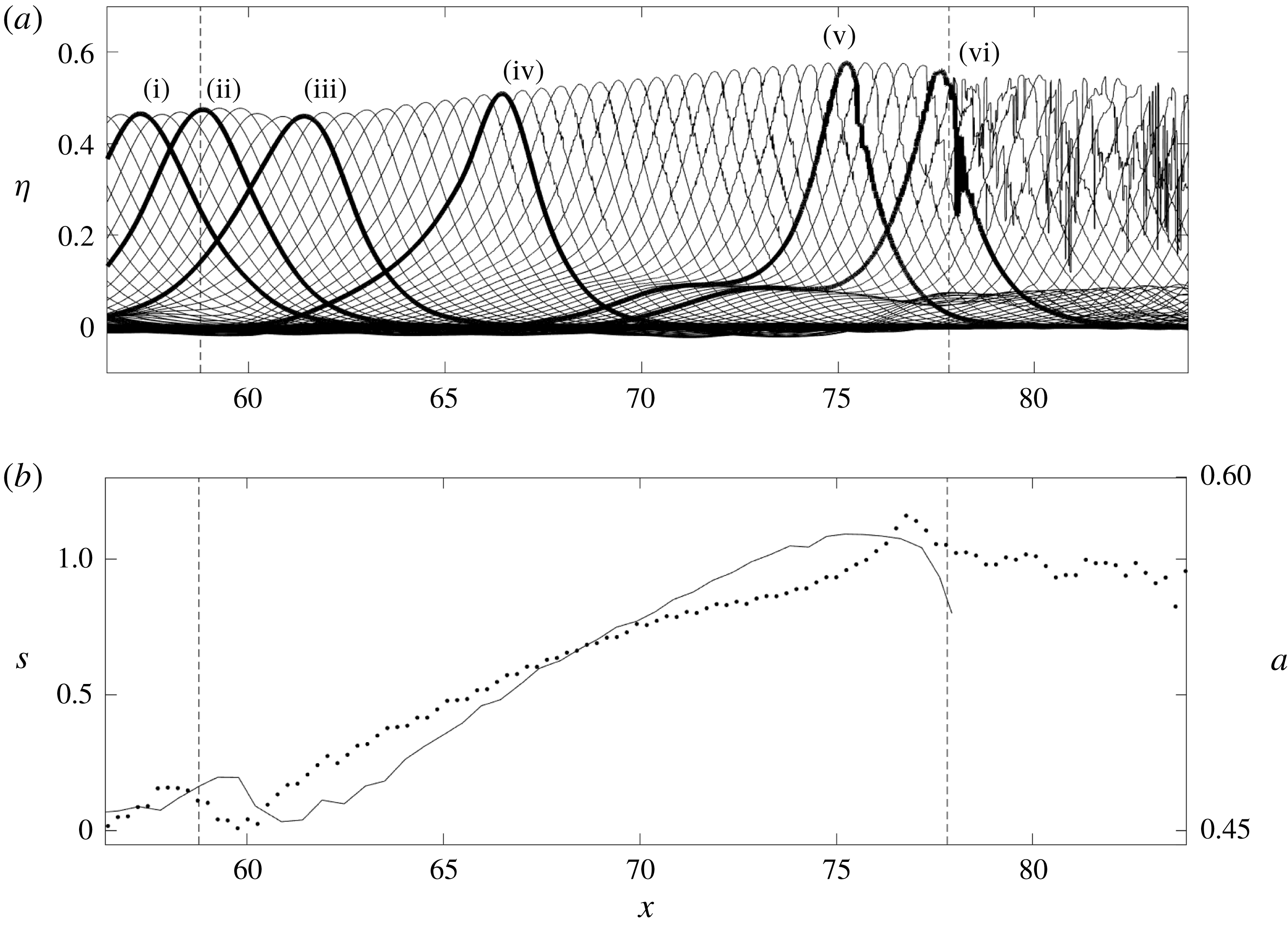
Figure 4(d) shows the wave amplitude evolution for the case shown in figure 3(d) compared to the unobstructed amplitude decay rate. The amplitude evolution shows the wave amplitude increases on the sill and decreases significantly after breaking. However, it is difficult to observe the detailed wave breaking process from the wave gauge measurement alone. Here we present the data acquired from the LIF technique applied in the local vicinity of the submerged sill. Figure 6(a) shows a waterfall plot for this case (
 $a_{i}=0.5,D/l=6.35$
). The vertical dashed lines represent the beginning and end of the submerged sill. Six time snaps of the waterfall plot are depicted in bold to represent different phases of the breaking process. Figure 6(b) shows the variation of the wave amplitude and the third moment of water-surface elevation
 $\unicode[STIX]{x1D702}$
, which represents the horizontal asymmetry of the wave profile. The normalized horizontal asymmetry,
 $s$
, is evaluated as
 $$\begin{eqnarray}\displaystyle s=\left.\int _{-\infty }^{\infty }(t-\overline{t})^{3}\unicode[STIX]{x1D702}\,\text{d}t\right/\left(\int _{-\infty }^{\infty }(t-\overline{t})^{2}\unicode[STIX]{x1D702}\,\text{d}t\right)^{3/2}, & & \displaystyle\end{eqnarray}$$
where
 $$\begin{eqnarray}\displaystyle \overline{t}=\left.\int _{-\infty }^{\infty }t\unicode[STIX]{x1D702}\,\text{d}t\right/\int _{-\infty }^{\infty }\unicode[STIX]{x1D702}\,\text{d}t. & & \displaystyle\end{eqnarray}$$
To compute the asymmetry, the integrals in (3.4) and (3.5) were approximated by taking the limits of
 $\pm \infty \rightarrow \pm t$
where
 $\unicode[STIX]{x1D702}\geqslant 0.1a$
. Note that a positive value of
 $s$
represents the waveform being tilted forward, and a negative value represents the waveform being tilted backward.
LIF measurements that show (a) a waterfall plot of the temporal water-surface profiles for a wave of amplitude
 $a_{i}=0.5$
which passes over a submerged sill of breadth
 $D/l=6.35$
(wide sill), and (b) variations of wave amplitude
 $a$
, ——, and the horizontal asymmetry,
 $s$
, computed by (3.4),
 $\cdots \cdots$
. The vertical dashed lines (– – –) represent the beginning and end of the submerged sill. The time interval in the profiles is
 $\unicode[STIX]{x0394}t=0.03~\text{s}$
. Six distinguished transformation stages (i) through (iv) in (a) are discussed in the text.

Examination of figure 6 illuminates the following characteristics in six phases:
(i) Incident wave upstream of the sill showing its symmetrical solitary-wave profile.
(ii) Slight increase in wave amplitude prior to the upstream edge due to the minute wave reflection.
(iii) Reduction in amplitude and increase in horizontal asymmetry immediately after crossing over the upstream edge.
(iv) Gradual increase in wave amplitude and asymmetry over the sill plateau; wave leans forward. Wave profile narrows and begins to show formation of single trailing dispersive wave. Here we observe the formation of roughness on the front face of the solitary wave. This surface roughness is interpreted as the appearance of capillary waves. Such formation of capillary waves prior to the wave breaking is known to be an indication of the onset of the development of a spilling breaker (Longuet-Higgins Reference Longuet-Higgins1994; Duncan et al. Reference Duncan, Qiao, Philomin and Wenz1999; Duncan Reference Duncan2001).
(v) Wave amplitude reaches its maximum amplification and begins to break. This occurs prior to the wave reaching its maximum horizontal asymmetry with a sharp increase. A small wave hump is formed on the lee side of the wave that will develop into a dispersive trailing wave.
(vi) Wave is broken and amplitude decreases. After the incipience of wave breaking, the horizontal asymmetry remains high: i.e. the waveform continues to be tilted forward with the breaking process.
3.4.2 Wave breaking downstream of sill
The case of a solitary wave with incident wave amplitude
 $a_{i}=0.6$
passing over a submerged sill of breadth
 $D/l=2.32$
(narrow sill) results in the occurrence of wave breaking downstream of the sill. Note that this is different than the previous case where the wave breaks on top of the sill (figure 6). Recall that the sill breadth in the previous case discussed in § 3.4.1 is
 $D/l=6.35$
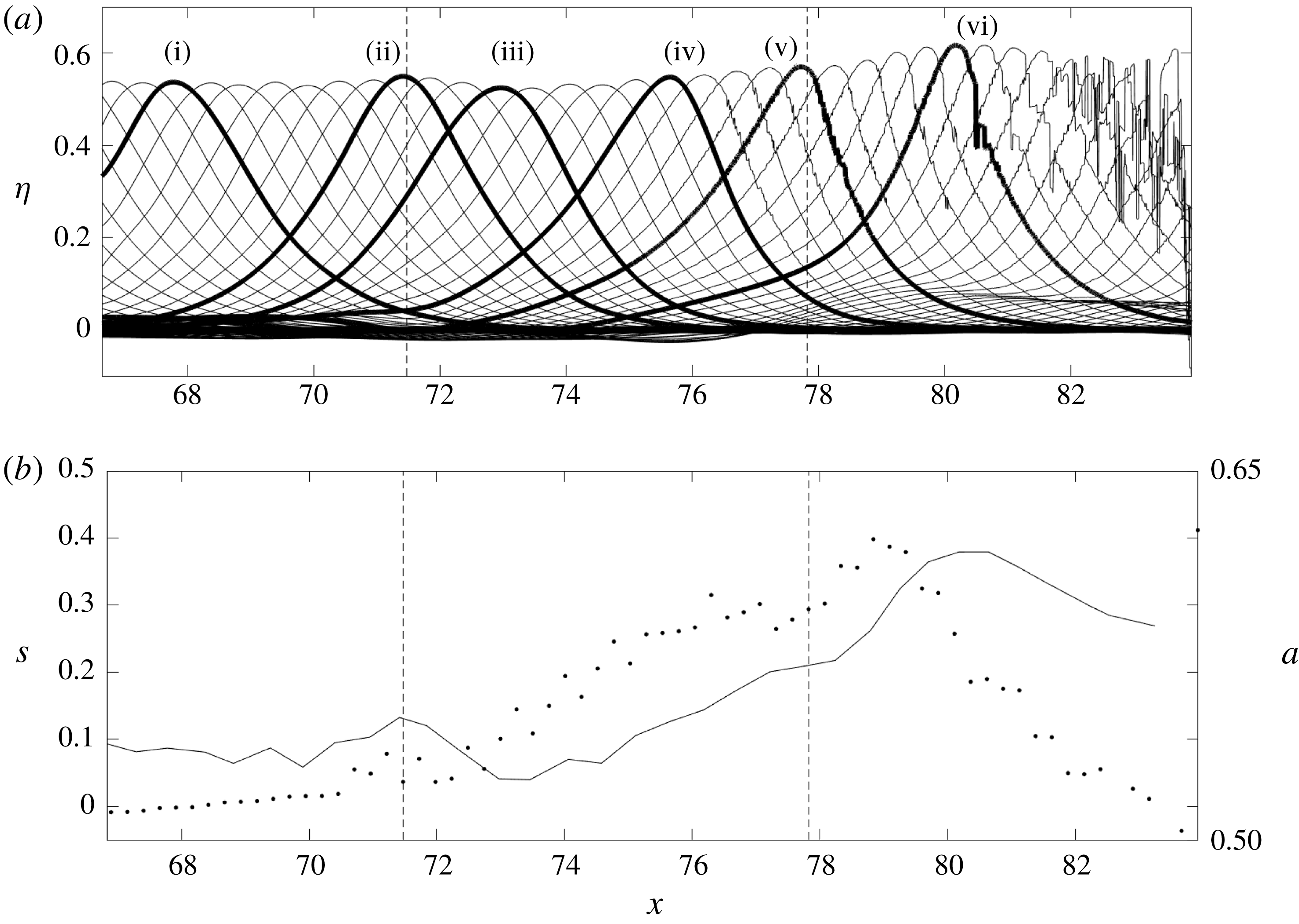
: substantially wider than this case. Figure 7 shows the LIF measurements performed in the local vicinity of the submerged sill. Figure 7(a) is a waterfall plot of the temporal wave profiles that shows the transformation of the wave leading to its breaking. The vertical dashed lines represent the beginning and end of the submerged sill. Six time snaps of the waterfall plot are depicted in bold to represent different phases of the breaking process, similar to the phases presented in figure 6.
LIF measurements that show (a) a waterfall plot of the temporal water-surface profiles for a wave of height
 $a_{i}=0.6$
which passes over a submerged sill of breadth
 $D/l=2.32$
(narrow sill), and (b) variations of wave amplitude
 $a$
, ——, and the horizontal asymmetry,
 $s$
, computed by (3.4),
 $\cdots \cdots$
. The vertical dashed lines (– – –) represent the beginning and end of the submerged sill. The time interval in the profiles is
 $\unicode[STIX]{x0394}t=0.03~\text{s}$
. Six distinguished transformation stages (i) through (iv) in (a) are discussed in the text.

Figure 7(b) shows the variation of wave amplitude and horizontal asymmetry evaluated by (3.4). Comparing the cases presented in figures 6 and 7, we notice that the wave amplitude of each case increases slightly prior to reaching the upstream edge of the sill, followed by an amplitude reduction once the wave crest climbs onto the sill. This slight amplitude increase and decrease must be related to the excess vertical component of velocity created by the upward step of the sill. The transmitted wave proceeds to shoal over the sill and increase in wave amplitude while decreasing in wavelength due to the shallower water on the plateau of the sill.
The wave breaking process is similar to that observed in figure 6(b), except that figure 7(b) shows that the breaking occurs downstream of the sill, instead of the location over the sill observed in figure 6(b). Note that the wave continues to increase in amplitude as it propagates beyond the downstream edge of the sill. This feature was observed by Cooker et al. (Reference Cooker, Peregrine, Vidal and Dold1990) and Grilli et al. (Reference Grilli, Losada and Martin1994) in their numerical experiments. More importantly, the wave asymmetry rapidly increases immediately after the downstream edge of the sill. The horizontal asymmetry reaches its maximum value prior to the occurrence of the maximum amplitude. This is opposite to the previous case of breaking demonstrated in figure 6, where the maximum asymmetry happens after the maximum wave amplification associated with the breaking incipience. The horizontal asymmetry reduces to nil, quickly recovering the symmetrical form of the solitary wave. This behaviour indicates that the breaking phenomenon for this case (
 $a_{i}=0.6$
,
 $D/l=2.32$
) lasts only for a short duration.
For the case where the wave breaks on top of the sill (figure 6), the wave amplitude increases until breaking, following typical shoaling behaviour. When
 $D/l$
is small (figure 7), the wave continues to increase in amplitude beyond the downstream edge of the sill until it breaks. When the wave is large, the wave deforms and tilts forward by the presence of the sill, which triggers the wave breaking. In other words, unlike the case shown in figure 6, the disturbance of the narrow sill causes this asymmetric deformation prior to the amplitude enhancement that eventually leads to the breaking at the leeside of the sill. The submerged sill forces the solitary wave to exceed a certain amplitude threshold which creates a nonlinear instability to lead wave breaking. This instability prevents the solitary wave from recovering and continues to grow regardless of whether or not the submerged sill is still underneath the wave crest. Since less time is spent on the sill, only waves with initially larger amplitudes can cross the instability threshold. Thus, for shorter breadths of the sill, only highly nonlinear waves break. We observe this in our experiments as only a solitary wave with its initial amplitude
 $a_{i}\gtrsim 0.59$
breaks over the narrow sill (
 $D/l=2.32$
). Note that this observation is based on a series of our experiments performed with
 $0.5\leqq a_{i}\leqq 0.6$
with the use of LIF, although clear identification of ‘breaking’ is subtle even with the LIF data analysis.
4 Discussion
To examine the effect of sill’s breadth, we isolate a specific wave amplitude. Figure 8 shows the temporal variations of the water surface
 $\unicode[STIX]{x1D702}$
measured at
 $x=74.7$
(above the sill: gauge location (6) as indicated in figure 1) and
 $x=126$
(near the end of the tank: gauge location (12)), respectively, for a wave with
 $a_{i}=0.3$
passing over each submerged sill configuration. The time axes for each of the individual time series are adjusted such that the profiles match up for more convenient comparison. Figure 8(a) shows that the wave amplification on the sill increases with sill breadth. Additionally, it appears that the wave leans forward and that trailing wave formation is more significant for wider sill breadths. Figure 8(b) shows that dispersive wave formation trailing the transmitted wave is apparent for all the cases with
 $a_{i}=0.3$
. The amplitude of the dispersive wavetrain increases as the length scale of the submerged sill increases. (Note that the leading crest elevations of the trailing wavetrain are 0.019, 0.025 and 0.045 for the cases of
 $D/l=1.64$
,
 $D/l=3.28$
and
 $D/l=4.93$
, respectively, although the values are not accurate owing to the resolution of the wave gauges
 ${\approx}0.18~\text{mm}$
). Figure 9 shows the comparison of amplitude evolutions between the cases with different sill breadths for a wave of
 $a_{i}=0.3$
. The amplitude on the sill increases and the downstream amplitude decreases with sill breadth: the sill breadth has a significant impact on the wave–sill response which in this case can vary from a small perturbation to a large perturbation. Figures 8 and 9 show that an increase in sill breadth can lead to larger perturbations. The maximum amplitude depends on the amount of time that the waves spend over the sill. All of the waves eventually recover to a solitary wave by the end of the wave tank with a small change in amplitude. Trailing waves are also similar but have higher amplitude for the cases with longer sill breadths.
Time variation of the water-surface elevation measured at (a)
 $x=74.7$
(downstream end of sill: the gauge location 6 (see figure 1)) and (b)
 $x=126.0$
(furthest propagation point in wave tank: the gauge location 12) for a wave with
 $a_{i}=0.3$
passing over each submerged sill configuration: ——, no sill; – – – –,
 $D/l=1.64$
; – ⋅ – ⋅ –,
 $D/l=3.28$
;
 $\cdots \cdots$
,
 $D/l=4.93$
. The time axes for each profile are adjusted such that the profiles match up for more convenient comparison.


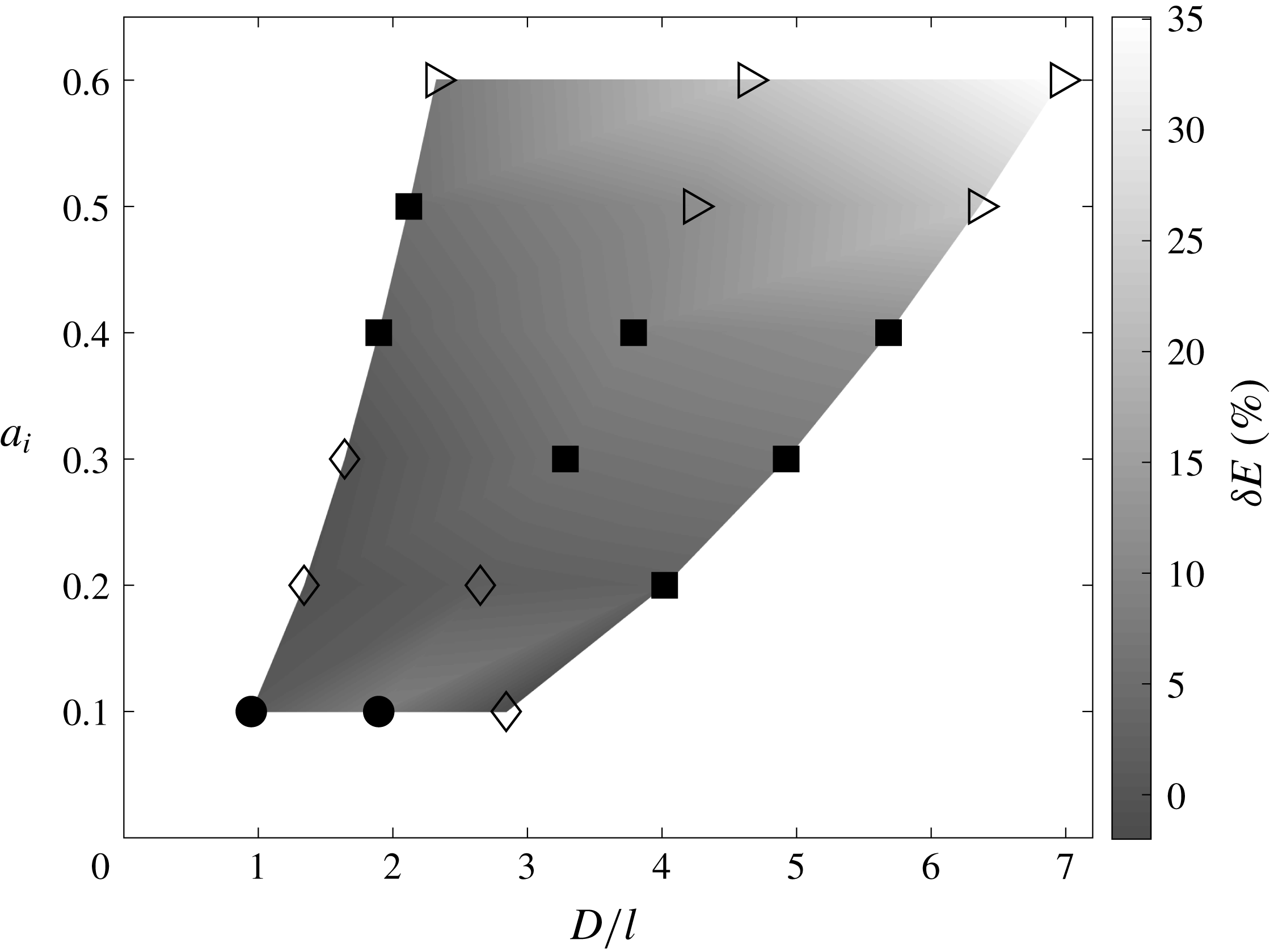
Figure 10 graphically presents the responses observed for the 18 experimental cases shown in table 1. The wave responses appear to depend on the effect of nonlinearity
 $a_{i}$
and the relative length scale
 $D/l$
. The type of response can be ranked based on the size of the perturbation such as (from small to large):
 $\text{unperturbed}\rightarrow \text{small perturbation}\rightarrow \text{large perturbation}\rightarrow \text{breaking}$
. As the perturbation increases, the solitary wave loses its ability to recover. This is first observed in the large perturbation case where the solitary-wave amplitude remains reduced (no recovery) far beyond the sill. When the perturbation becomes sufficiently large, the perturbation continues to grow beyond the sill until the wave breaks. From figure 10, we can see that the size of perturbation increases with both parameters
 $D/l$
and
 $a_{i}$
. Note that for solitary waves,
 $a_{i}$
and
 $l$
are not independent. A larger wave amplitude,
 $a_{i}$
, corresponds to a shorter wavelength,
 $l$
. Since wavelength is proportional to
 $a_{i}^{-1/2}$
, sill breadth,
 $D/l$
, increases as
 $a_{i}$
increases. Thus, the length scale of the submerged sill has a clear effect on the type of transformation that the solitary wave experiences over the sill.
Solitary-wave responses observed for the 18 experimental cases, also listed in table 1: ●, unperturbed; ♢, small perturbation; ◼, large perturbation; ▹, wave breaking. The background grey shade represents energy losses
 $\unicode[STIX]{x1D6FF}E$
relative to the corresponding unobstructed solitary wave: see table 1.

Figure 10 expresses per cent (%) losses
 $\unicode[STIX]{x1D6FF}E$
of mechanical energy relative to the corresponding unobstructed solitary wave. The energies are computed by (3.3) and listed in table 1. The resulting relative energy loss indicates that the longer the
 $D/l$
the greater the loss. The loss sharply increases for the breaking-wave cases due to energy dissipation associated with the induced turbulence. Among the breaking-wave cases, energy dissipation turns out to be smaller when
 $D/l$
is small than that for when
 $D/l$
is large. For the cases presented in § 3.4, the relative energy dissipation for the case of breaking over the wide sill (
 $D/l=6.35$
) is 23.1 %, which is significantly larger than the 7.1 % dissipation for the case where breaking occurred downstream of the narrow sill (
 $D/l=2.32$
). For a short-breadth sill, while some energy dissipates by breaking, most of the energy must be recovered immediately after the wave passes over the sill. On the other hand, the wide sill sustains continual wave breaking for a long time, which allows for sufficient dissipation. As discussed in §§ 3.4.1 and 3.4.2, the variation of the horizontal asymmetry,
 $s$
, differed based on the value of
 $D/l$
. When
 $D/l$
is small, the increase in horizontal asymmetry is temporary and the symmetrical waveform is recovered quickly after breaking. When
 $D/l$
is large, the value of
 $s$
persists with wave breaking after the wave passes over the sill.
For non-breaking cases, the energy reduction must result from energy dissipation through turbulence associated with flow separation caused at the salient edges of the sill, as well as energy reflection and dispersion in the form of a trailing wavetrain. The amount of energy reduction is much smaller for non-breaking waves cases than for the breaking waves cases.
5 Conclusions
Laboratory experiments are performed to study the effect of a rectangular-shaped broad sill on solitary-wave deformation and evolution during and after passing through a sill. Based on the experimental results, the following conclusions are drawn:
(i) Four different responses of solitary waves are identified. They are classified as ‘unperturbed’, ‘small perturbation’, ‘large perturbation’ and ‘wave breaking’. These different interactions are described in § 3. For very small perturbations (classified as ‘unperturbed’), the solitary wave does not appear to be affected at all. For small perturbations, the solitary wave amplitude is locally amplified but recovers to its initial state with the formation of small dispersive trailing waves. As the perturbations get larger, the solitary-wave amplitude does not recover entirely and a noticeable trailing dispersive wavetrain is formed. At a certain size, the perturbations cause the wave to break.
(ii) The different wave responses depend largely on the wave amplitude and sill breadth, and can be divided up into regions of the
 $(a_{i},D/l)$
parameter space (see figure 10).
(iii) For a single wave amplitude
$a_{i}=0.3$
, the sill breadth has a clear effect on amplification of the wave amplitude and the type of wave response that occurs (see § 4).(iv) Detailed wave transformation leading to wave breaking by the presence of the sill is captured with the use of the LIF technique. Considering the amplitude and horizontal asymmetry variations, the observed pre-breaking behaviours can be explained by the effect of amplitude dispersion. The tilted sawtooth-like wave formation enhances the instability that leads to breaking. The relative timing of the maximum wave amplitude to peak horizontal asymmetry differed based on where the wave breaking occurred relative to the sill. For the case where wave breaking occurred on top of the sill, the maximum amplitude precedes the peak horizontal asymmetry, and the asymmetry persists with a prolonged wave-breaking process that results in substantial energy dissipation. When the wave breaking occurs beyond the downstream edge of the sill, however, the peak horizontal asymmetry precedes the maximum amplitude and the asymmetry subsides to nil, quickly recovering its solitary-wave form.


Acknowledgement
This work was partially supported by the US National Science Foundation (OCE-1830024).