



1. Introduction
The gravity-driven flow of a liquid film along a vertical cylindrical fibre represents a fundamental paradigm in interfacial hydrodynamics, distinguished from its planar counterpart by the presence of transverse curvature. While ubiquitous in applications ranging from optical fibre coating to desalination (Sadeghpour et al. Reference Sadeghpour, Zeng, Ji, Dehdari Ebrahimi, Bertozzi and Ju2019; Onsager Reference Onsager2022; Aksoy et al. Reference Aksoy, Yılmaz, Maleki, Rahbar and Barani2024; Chao et al. Reference Chao, Zhu, Ding, Kong, Chang and Wang2024), the utility of such flows is intrinsically limited by the spontaneous breakup of the interface into a beads-on-a-string structure, which dictates the operational limits of coating quality and speed (Quéré Reference Quéré1990; Kliakhandler et al. Reference Kliakhandler, Davis and Bankoff2001). The stability of this system is governed by the interplay between two distinct physical mechanisms. The first is the Rayleigh–Plateau instability (Plateau Reference Plateau1873; Rayleigh Reference Rayleigh1878, Reference Rayleigh1892), driven by the azimuthal curvature associated with the geometric confinement (Kalliadasis & Chang Reference Kalliadasis and Chang1994; Chang & Demekhin Reference Chang and Demekhin1999); physically, this arises as surface tension acts to minimise the free-surface area by amplifying axisymmetric perturbations. The second is the hydrodynamic or Kapitza mode (Kapitza Reference Kapitza1948; Benjamin Reference Benjamin1957), a dynamic instability arising from the competition between inertia, gravity and viscosity, analogous to the surface waves observed in planar falling films (Duprat et al. Reference Duprat, Ruyer-Quil and Giorgiutti-Dauphiné2009; Ruyer-Quil & Kalliadasis Reference Ruyer-Quil and Kalliadasis2012). Theoretical characterisation of the coupling between these geometric and hydrodynamic modes is essential for predicting the nonlinear topological transitions of the interface.
Early research on fibre coating focused primarily on predicting the entrained film thickness during wire withdrawal. Tallmadge et al. (Reference Tallmadge, Labine and Wood1965) and De Ryck & Quéré (Reference De Ryck and Quéré1996) characterised the coating laws across viscous and inertial regimes, establishing the dependence of film thickness on capillary and Weber numbers, respectively. Beyond the determination of film thickness, a more fundamental question concerns the hydrodynamic stability of such annular films. The foundational stability analysis was established by Goren (Reference Goren1962), who demonstrated that surface tension inevitably drives the film to break up into a regular array of droplets, with the selected wavelength governed strictly by the film-to-fibre-radius ratio. Significantly, Lin & Liu (Reference Lin and Liu1975) further elucidated the physical mechanism governing this breakup, framing it as a dynamic competition between the destabilising capillary pinching force (associated with azimuthal curvature) and the stabilising capillary restoring force (associated with axial curvature). Advancing this understanding into the nonlinear regime, Kalliadasis & Chang (Reference Kalliadasis and Chang1994) identified a critical thickness threshold that governs the ultimate topological fate of the interface: below this limit, the instability saturates into finite-amplitude solitary waves, whereas above it, the film undergoes accelerated growth characterised by a self-similar blow-up, leading to the formation of large localised drops. Building on this foundation, Chang & Demekhin (Reference Chang and Demekhin1999) further elucidated the specific dynamical mechanism of drop formation in the supercritical regime, characterising it as a self-growth process driven by a substrate jump. Their study demonstrates that a supercritical pulse advances into a thicker precursor film while leaving behind a thinner trailing substrate, and this imbalance in mass flux drives the pulse amplitude towards an accelerated growth regime characterised by a self-similar blow-up.
Experimentally, Kliakhandler et al. (Reference Kliakhandler, Davis and Bankoff2001) identified three distinct wave regimes in experiments based on differences in film flow rate and morphology: large-amplitude solitary waves with wide separation (Regime A), closely packed periodic necklace waves (Regime B) and irregular sliding droplets at low flow rates (Regime C). They derived an evolution equation based on the full curvature assumption, which effectively captured the dynamics dominated by gravity and surface tension under creeping flow conditions. Craster & Matar (Reference Craster and Matar2006) subsequently utilised lubrication approximation and asymptotic expansion to derive a nonlinear equation applicable to the long-wave limit. Their numerical solutions not only successfully reproduced the three experimentally observed regimes but also revealed, through bifurcation analysis, a multiple-solution structure involving single-, double- and triple-droplet states as the computational domain varied. To extend the applicability of the model to a broader parameter space (including moderate Reynolds numbers and the short-wave region), Ruyer-Quil et al. (Reference Ruyer-Quil, Treveleyan, Giorgiutti-Dauphiné, Duprat and Kalliadasis2008) established a low-dimensional two-equation model for flow rate
 $q$
and film thickness
 $h$
based on the boundary-layer approximation and the weighted residual method. By incorporating high-order effects such as streamwise viscous dispersion, this model clearly classified the film dynamics into four physical regimes: (i) the drag–gravity regime dominated by gravity and viscous drag; (ii) the drag–inertia regime; (iii) the drop-like regime dominated by azimuthal curvature and forming symmetric droplets; and (iv) the soliton-like regime sustained by the balance between nonlinearity and second-order viscous dispersion. This duality of physical mechanisms maps directly onto the nature of spatiotemporal instability: the gravity-driven advection effect tends to enhance the downstream transport of disturbances (promoting convective instability), whereas the Rayleigh–Plateau mode, dominated by surface tension, provides the necessary upstream propagation mechanism and serves as the key driver triggering absolute instability (AI). This spatiotemporal instability framework was first established by Duprat et al. (Reference Duprat, Ruyer-Quil, Kalliadasis and Giorgiutti-Dauphiné2007, Reference Duprat, Ruyer-Quil and Giorgiutti-Dauphiné2009), who, through a combination of experiment and theory, revealed that AI originates precisely when the Rayleigh–Plateau mechanism overcomes gravity-driven advection, typically occurring within an intermediate range of film thicknesses on thin fibres. Building on this, Ruyer-Quil & Kalliadasis (Reference Ruyer-Quil and Kalliadasis2012) further pointed out that the drop-like regime dominated by surface tension inherently corresponds to AI, while the drag–gravity regime dominated by advection corresponds to convective instability (CI).
Within the regime of AI, the interface response to pulse perturbations is often characterised by sustained local growth and, in sufficiently nonlinear stages, by film rupture. Unlike convective evolution, where disturbances are amplified while being swept downstream, AI allows disturbances to remain and grow near their source, thereby providing a route towards a contact singularity. As the system approaches rupture (
 $t \rightarrow t_c$
), the minimum film thickness commonly follows a self-similar law,
 $h_{\textit{min}} \sim (t_c - t)^m$
, whose exponent depends on the dominant force balance (Eggers Reference Eggers1997). For surface-tension-driven free jets or droplets, inertial–capillary thinning gives a
 $2/3$
power law, whereas viscous–capillary thinning leads to the linear scaling
 $m=1$
(Papageorgiou Reference Papageorgiou1995; Eggers Reference Eggers1997). For annular films coating a fibre, the presence of a rigid wall changes the flow topology: Lister et al. (Reference Lister, Rallison, King, Cummings and Jensen2006) showed that drainage is governed by a squeezing motion resisted by wall friction, rather than by the extensional thinning of a free jet. In the absence of gravity, this Newtonian annular-film drainage nevertheless retains a linear scaling. This scaling can be altered by additional physical effects, such as intermolecular forces at microscopic scales (Williams & Davis Reference Williams and Davis1982; Dallaston et al. Reference Dallaston, Fontelos, Tseluiko and Kalliadasis2018) or nonlinear Maxwell stresses under a radial electric field (Liu et al. Reference Liu, Chen and Ding2018). However, it remains unclear how viscoelasticity, within a fibre-coating geometry where Rayleigh–Plateau growth competes with gravity-driven advection, affects not only the temporal growth of disturbances but also their convective or absolute character and subsequent nonlinear evolution.
To address this question, we investigate the stability and nonlinear dynamics of a viscoelastic liquid film flowing down a vertical fibre, using the Walters’ liquid B model to describe elastic effects. The central aim is to determine how viscoelasticity modifies the instability, wave propagation and nonlinear evolution of a liquid film flowing down a vertical fibre, where interfacial curvature drives the Rayleigh–Plateau instability while gravity advects disturbances downstream. We combine a long-wave asymptotic model, a weighted Orr–Sommerfeld stability analysis and numerical simulations of the nonlinear evolution equation. This framework allows us to examine three connected aspects of the problem. First, we quantify how elasticity modifies the temporal instability and compare the asymptotic predictions with the Orr–Sommerfeld results. Second, we map the transition between CI and AI in the parameter space of elasticity, geometric confinement and gravity, showing that elasticity can shift the AI/CI boundary rather than merely changing the local temporal growth rate. Third, we follow the nonlinear evolution in the absolutely unstable regime, including finite-time thinning and travelling-wave states, to determine how the elasticity-modified instability is manifested beyond the linear stage. The remainder of the paper is organised as follows. In § 2, we formulate the mathematical model based on the Walters’ liquid B constitutive equation, derive the long-wave evolution equation and present the weighted Orr–Sommerfeld system together with the AI/CI criterion. In § 3, we analyse the temporal and spatiotemporal stability, compare the long-wave and Orr–Sommerfeld predictions and construct the CI/AI boundaries in the
 $(a,Bo)$
parameter space. In § 4, we examine the nonlinear dynamics, including wave saturation, rupture scaling and travelling-wave phase-space structures. Conclusions are given in § 5.
2. Mathematical formulation and stability methods
Schematic of a viscoelastic liquid film coating a vertical cylindrical fibre of radius
 $a_0$
. The film, with initial thickness
 $h_0$
, flows downward under gravity
 $g$
along the
 $z$
axis. The deformable free surface
 $h(z,t)$
is subject to axisymmetric perturbations of wavelength
 $\lambda _0$
.

We consider the gravity-driven flow of a weakly viscoelastic liquid film coating the exterior of a vertical cylindrical fibre of radius
 $a_0$
, as schematically illustrated in figure 1. The liquid is characterised by density
 $\rho$
and viscosity
 $\mu$
. The liquid film has an initial thickness
 $h_0$
and flows downwards along the vertical
 $z$
axis under gravity
 $g$
. Subjecting the initially uniform film to a small-amplitude perturbation of wavelength
 $\lambda _0$
, we denote the perturbed liquid–gas interface by
 $h(z, t)$
. The flow is assumed to be axisymmetric (
 $\partial /\partial \theta = 0$
) in cylindrical coordinates
 $(r, z)$
, bounded internally by the solid fibre surface and externally by the deformable free surface. To characterise the weak elastic effect, we adopt the Walters’ liquid B viscoelastic model, which serves as a first-order elastic correction to the Newtonian framework.
The governing equations of the flow consist of the mass and momentum conservation equations, supplemented by the constitutive relation of the Walters’ liquid B model. The dimensional conservation equations are
 \begin{align} \boldsymbol{\nabla }\boldsymbol{\cdot }\boldsymbol{V} &=0,\,\,\,\,\, \\[-28pt] \nonumber \end{align}
 \begin{align} \rho \left [\frac {\partial \boldsymbol{V}}{\partial t} + \left (\boldsymbol{V} \boldsymbol{\cdot }\boldsymbol{\nabla }\right ) \boldsymbol{V} \right ] &= -\boldsymbol{\nabla }p + \boldsymbol{\nabla }\boldsymbol{\cdot }\boldsymbol{\tau } + \rho \boldsymbol{g}, \\[0pt] \nonumber \end{align}
where
 $\boldsymbol{V}=(u,w)$
is the velocity field in
 $(r,z)$
and
 $p$
is the pressure. The extra-stress tensor of the Walters’ liquid B model is given by
 \begin{align} \boldsymbol{\tau} =2 \mu \boldsymbol{D} - 2M_0 \overset{\nabla}{\boldsymbol{D}}, \end{align}
where the strain rate tensor
 $\boldsymbol{D}=({1}/{2}) [\boldsymbol{\nabla }\boldsymbol{V}+ ( \boldsymbol{\nabla }\boldsymbol{V} )^T ]$
, and
 $\overset {\boldsymbol{\nabla }}{\boldsymbol{D}}$
denotes the upper-convected derivative:
 \begin{align} \overset {\boldsymbol{\nabla }}{\boldsymbol{D}}=\frac {\partial \boldsymbol{D}}{\partial t}+\boldsymbol{V}\boldsymbol{\cdot }\boldsymbol{\nabla }\boldsymbol{D}-\left (\boldsymbol{\nabla }\boldsymbol{V}\right )^T\boldsymbol{\cdot }\boldsymbol{D}-\boldsymbol{D}\boldsymbol{\cdot }\boldsymbol{\nabla }\boldsymbol{V}. \end{align}
The material parameter
 $M_0$
quantifies the elastic contribution, and the model reduces exactly to a Newtonian case with viscosity
 $\mu$
when
 $M_0 = 0$
.
We consider a slender-film regime, where the characteristic radial scale
 $R = a_0 + h_0$
is much smaller than the axial scale
 $L$
. Balancing viscous and capillary forces yields the capillary length
 $L = \sigma /(\rho g R)$
, where
 $\sigma$
denotes the surface tension coefficient. This introduces the slenderness parameter
 $\varepsilon = R/L \ll 1$
. The characteristic velocity is scaled as
 $U = \rho g R^2/\mu$
. The dimensionless variables (denoted by asterisks) are defined as
 \begin{align} a^*=\frac {a_0}{R}, \quad r^*=\frac {r}{R}, \quad z^*=\frac {z}{L},\quad p^*=\frac {p}{\rho g L},\quad t^*=\frac { U t}{L},\quad w^*=\frac {w}{U},\quad u^*= \frac {u}{\varepsilon U}. \end{align}
Note that the radial velocity is scaled by
 $\varepsilon$
to satisfy continuity. Consequently, the Bond number
 $\textit{Bo} = \rho g R^2/\sigma$
is equivalent to
 $\varepsilon$
, representing the relative importance of gravity to surface tension. Dropping the asterisks for brevity, the axisymmetric continuity and momentum equations take the form
 \begin{align} \frac {1}{r} \frac {\partial }{\partial r} (r u) + \frac {\partial w}{\partial z} = 0, \\[-28pt] \nonumber \end{align}
 \begin{align} \varepsilon ^4 Re \left (\frac {\partial u}{\partial t} + u \frac {\partial u}{\partial r} + w \frac {\partial u}{\partial z}\right ) = -\frac {\partial p}{\partial r} + \frac {1}{r} \frac {\partial }{\partial r} (r \tau _{rr}) + \varepsilon \frac {\partial \tau _{zr}}{\partial z} - \frac {\tau _{\theta \theta }}{r}, \\[-28pt] \nonumber \end{align}
 \begin{align} \varepsilon ^2 Re \left (\frac {\partial w}{\partial t} + u \frac {\partial w}{\partial r} + w \frac {\partial w}{\partial z} \right ) = -\frac {\partial p}{\partial z} + \frac {1}{\varepsilon r} \frac {\partial }{\partial r} (r \tau _{rz}) + \frac {\partial \tau _{zz}}{\partial z} + 1. \\[-12pt] \nonumber \end{align}
Here,
 $\textit{Re}=\rho U R/\mu$
is the Reynolds number based on radial scale and
 $\tau _{ij}$
are the components of the extra-stress tensor. Since
 $\tau _{rz}=O(\varepsilon )$
in the slender-film approximation, the term
 $( {1}/{\varepsilon r})( {\partial }/{\partial r}) (r \tau _{rz})$
is of order
 $O(1)$
. The explicit expressions of the stress components are given as follows:
 \begin{align} \begin{aligned} \tau _{rr} & = 2 \varepsilon ^2 \frac {\partial u}{\partial r} - \varepsilon ^3 M \Bigg [2\frac {\partial ^2 u}{\partial t \partial r} + 2 u \frac {\partial ^2 u}{\partial r^2} -2 w \left (\frac {\partial ^2 w}{\partial z^2}+\frac {1}{r}\frac {\partial u}{\partial z}\right ) \\& \quad - 4 \left ( \frac {\partial u}{\partial r} \right )^2-2\frac {\partial u}{\partial z}\frac {\partial w}{\partial r}-2\varepsilon ^2\left ( \frac {\partial u}{\partial z} \right )^2\Bigg ], \end{aligned} \\[-28pt] \nonumber \end{align}
 \begin{align} \begin{aligned} \tau _{rz} & = \left ( \varepsilon ^3\frac {\partial u}{\partial z} + \varepsilon \frac {\partial w}{\partial r} \right ) - \varepsilon ^2 M \bigg [\varepsilon ^2\frac {\partial ^2 u}{\partial z \partial t}+\frac {\partial ^2 w}{\partial r \partial t}-\varepsilon ^2 u\left (\frac {\partial ^2 w}{\partial z^2}+\frac {1}{r}\frac {\partial u}{\partial z}\right ) + u \frac {\partial ^2 w}{\partial r^2}\\& \quad +\varepsilon ^2 w \frac {\partial ^2 u}{\partial z^2}+ w\left ( \frac {u}{r^2} - \frac {1}{r}\frac {\partial u}{\partial r} -\frac {\partial ^2 u}{\partial r^2}\right )-2\frac {\partial u}{\partial r}\frac {\partial w}{\partial r} \nonumber \\& \quad +\frac {u}{r}\left (\varepsilon ^2\frac {\partial u}{\partial z}+\frac {\partial w}{\partial r}\right )-2\varepsilon ^2\frac {\partial u}{\partial z}\frac {\partial w}{\partial z} \bigg ], \end{aligned} \\[-28pt] \nonumber \end{align}
 \begin{align} \tau _{\theta \theta } = 2 \varepsilon ^2 \frac {u}{r} - \varepsilon ^3 M \left [\frac {2}{r}\frac {\partial u}{\partial t}+ 2u \left (\frac {1}{r}\frac {\partial u}{\partial r}-\frac {u}{r^2}\right )+2\frac {w}{r}\frac {\partial u}{\partial z}-4\frac {u^2}{r^2}\right ], \\[-28pt] \nonumber \end{align}
 \begin{align} \begin{aligned} \tau _{zz} & = 2\varepsilon ^2 \frac {\partial w}{\partial z} - \varepsilon M \Bigg [ 2\varepsilon ^2\frac {\partial ^2 w}{\partial z\partial t} + 2\varepsilon ^2\frac {u^2}{r^2}- 2 \varepsilon ^2 \frac {u}{r}\frac {\partial u}{\partial r}-2 \varepsilon ^2 u\frac {\partial ^2 u}{\partial r^2} \\& \quad +2\varepsilon ^2 w\frac {\partial ^2 w}{\partial z^2} -2\varepsilon ^2\frac {\partial w}{\partial r}\frac {\partial u}{\partial z}-2\left (\frac {\partial w}{\partial r}\right )^2-4\varepsilon ^2\left (\frac {\partial w}{\partial z}\right )^2 \Bigg ]. \end{aligned} \\[0pt] \nonumber \end{align}
The definition of the scaled elasticity parameter as
 $M = L M_0 / (\varepsilon \mu U)$
is a mathematical necessity driven by the asymptotic structure of the governing equations. In the slender-film limit, the dominant shear term in the axial momentum equation takes the form
 $({1}/{\epsilon r})( {\partial }/{\partial r})(r\tau _{rz})$
. When expanding the viscoelastic shear stress
 $\tau _{rz}$
, the Newtonian viscous contribution appears at
 $O(\epsilon )$
, while the leading elastic normal stress effects appear at
 $O(\epsilon ^2)$
. Inserting these expansions into the momentum equation results in the Newtonian viscous force acting at
 $O(1)$
and the elastic force acting at
 $O(\epsilon M)$
. To ensure that elasticity acts as a first-order perturbation – thereby preserving the classical Newtonian base flow at
 $O(1)$
– the parameter
 $M$
must be
 $O(1)$
. Therefore, we invoke the weakly viscoelastic assumption, which presumes that the natural elasticity group of the fluid,
 $L M_0 / (\mu U)$
, scales as
 $O(\varepsilon )$
. Defining
 $M$
as the natural group divided by
 $\varepsilon$
guarantees that
 $M \sim O(1)$
.
Typical material properties validate the proposed scaling. For a Walters’ liquid B fluid (e.g. poly(methyl methacrylate) in pyridine with
 $\rho = 980 \ \text{kg}\ \text{m}^{-3}$
,
 $M_0 = 0.04 \ \text{N}\ \text{s}^2 \ \text{m}^{-2}$
and surface tension
 $\sigma \approx 0.038 \ \text{N}\ \text{m}^{-1}$
; Walters Reference Walters1960; Du et al. Reference Du, Xiao, Wang, Zeng and Zhao2024) flowing with a characteristic total radius
 $R = a_0 + h_0 = 0.8 \ \text{mm}$
, the slenderness parameter evaluates to
 $\varepsilon \approx 0.16$
. The natural elasticity group evaluates to
 $L M_0 / (\mu U) \equiv \sigma M_0 / [(\rho g)^2 R^3] \approx 0.032$
. Dividing the natural group by
 $\varepsilon$
yields a physical baseline of
 $M \approx 0.20$
, establishing that
 $M$
operates within the
 $O(1)$
regime. Building upon the calculated baseline, our theoretical analyses explore a broader parameter space (varying
 $M$
up to a maximum of
 $0.5$
). Extending the parameter range allows us to elucidate the influence of elastic effects while remaining within the bounds of the weakly viscoelastic
 $O(1)$
scaling framework.
The system is closed by the following boundary conditions. At the fibre surface
 $r = a$
, the no-slip and no-penetration conditions require
 \begin{align} u=0, w = 0. \end{align}
At the free surface
 $r = a+h(z,t)$
, both the kinematic and dynamic boundary conditions must be satisfied. The kinematic boundary condition enforces that material points on the interface move with the fluid velocity, yielding
 \begin{align} u=\partial _t h + w\partial _z h. \end{align}
The dynamic conditions correspond to the balance of normal and tangential stresses on the deformable interface. Then the normal-stress balance takes the form
 \begin{align} - p + \frac {\tau _{rr} -2\varepsilon \partial _z h \tau _{rz} + \varepsilon ^2\left (\partial _z h\right )^2\tau _{zz}}{1 + \left (\varepsilon ^2\partial _z h\right )^2} =\frac {-(a+h)^{-1}}{\left [1+\varepsilon ^2\left (\partial _z h\right )^2\right ]^{1/2}}+\frac {\varepsilon ^2 \partial _{zz} h}{\left [1+\varepsilon ^2\left (\partial _z h\right )^2\right ]^{3/2}}. \end{align}
Similarly, the tangential-stress balance yields
 \begin{align} \partial _z h \left ( \tau _{rr} - \tau _{zz}\right ) + \frac {1}{\varepsilon }\big [1 - \varepsilon ^2 (\partial _z h)^2\big ] \tau _{rz} = 0. \end{align}
2.1. Asymptotic base state and long-wave evolution equation
To derive a reduced one-dimensional model under the slender-film assumption
 $\varepsilon \ll 1$
, the velocity and pressure fields are expanded as regular series in
 $\varepsilon$
:
 \begin{align} f = f_0 + \varepsilon f_1 + O(\varepsilon ^2), \quad \text{for } f \in \{u, w, p\}. \end{align}
The leading-order terms
 $(u_0, w_0, p_0)$
describe the Newtonian lubrication limit, while the
 $O(\varepsilon )$
corrections account for the weak viscoelastic effects. Substituting these expansions into the governing equations and retaining terms of
 $O(1)$
yields the leading-order axisymmetric lubrication equations:
 \begin{align} \frac {\partial r u_0}{r \partial r}+\frac {\partial w_0}{\partial z}=0, \quad \frac {\partial p_0}{\partial r} =0, \quad -\frac {\partial p_0}{\partial z}+\frac {\partial ^2 w_0}{\partial r^2}+\frac {1}{r}\frac {\partial w_0}{\partial r}+1 =0. \end{align}
The corresponding leading-order boundary conditions are
 \begin{align} u_0=0, \quad w_0=0, \quad \text{at} \; r=a; \\[-28pt] \nonumber \end{align}
 \begin{align} p_0=\frac {1}{a+h}-\varepsilon ^2 \partial _{zz} h, \quad \frac {\partial w_0}{\partial r}=0, \quad \text{at} \; r=a+h(z,t). \\[0pt] \nonumber \end{align}
Integrating (2.11) subject to (2.12) yields the leading-order velocity and pressure distributions:
 \begin{align} p_0=\frac {1}{a+h}-\varepsilon ^2 \partial _{zz} h, \\[-28pt] \nonumber \end{align}
 \begin{align} \begin{aligned} u_0 & = \frac {1}{16r}\bigg \{4\left (a+h\right ) \left (a^2-r^2+2r^2\ln \frac {r}{a}\right ) \left (\partial _z p_{0}-1 \right )\partial _z h \\& \quad + \left [-\big (a^2-r^2\big )^2+2\left (a+h\right )^2\left (a^2-r^2+2r^2\ln \frac {r}{a}\right ) \right ] \partial _{zz} p_{0}\bigg \}, \end{aligned} \\[-28pt] \nonumber \end{align}
 \begin{align} w_0 =\frac {\partial _z p_0-1}{4} \big [r^2-a^2 - 2(a+h)^2 (\ln r-\ln a)\big ]. \\[-12pt] \nonumber \end{align}
The set of equations (2.13) describes a capillary–gravity-driven Poiseuille flow, modified by azimuthal and axial curvatures of the fibre. The
 $O(\varepsilon )$
contributions incorporate the influence of fluid elasticity. The first-order governing equations are
 \begin{align} \frac {\partial r u_1}{r \partial r}+\frac {\partial w_1}{\partial z}=0, \quad \frac {\partial p_1}{\partial r} =0, \\[-28pt] \nonumber \end{align}
 \begin{align} -\frac {\partial p_1}{\partial z}+\frac {1}{r}\frac { \partial r G(r,h)}{\partial r}+4M\frac {\partial w_0}{\partial r}\frac {\partial ^2 w_0}{\partial r \partial z} =0, \\[0pt] \nonumber \end{align}
where
 $G(r,h)$
denotes the modified shear rate containing viscoelastic contributions:
 \begin{align} G(r,h)=\frac {\partial w_1}{\partial r}-M H(r,h). \end{align}
Here, the viscoelastic history effects are encapsulated in
 $H(r,h)$
, defined as
 \begin{align} H(r,h)=\frac {\partial ^2 w_0}{\partial r \partial t}+u_0 \frac {\partial ^2 w_0}{\partial r^2}+w_0\left (\frac {u_0}{r^2}-\frac {\partial u_0}{r \partial r}-\frac {\partial ^2 u_0}{\partial r^2}\right )-2\frac {\partial u_0}{ \partial r}\frac {\partial w_0}{\partial r}+\frac {u_0}{r}\frac {\partial w_0}{\partial r}. \end{align}
The
 $O(\varepsilon )$
boundary conditions are derived by expanding the no-slip condition at the fibre surface and the stress balances at the free surface:
 \begin{align} u_1=0, \quad w_1=0, \quad \text{at} \; r=a; \\[-28pt] \nonumber \end{align}
 \begin{align} p_1=0, \quad G(r, h)=2 M \partial _z h \left (\frac {\partial w_0}{\partial r}\right )^2, \quad \text{at} \; r=a+h(z,t). \\[0pt] \nonumber \end{align}
Solving equation (2.14) subject to the boundary conditions (2.17) yields the first-order solution, which represents the weak-elasticity correction to the Newtonian base state:
 \begin{align} G(r,h) & = \frac {M(1-\partial _z p_0)\partial _{zz} p_0}{4r}\left [(a+h)^4\left (3-4\ln \frac {a+h}{r}\right )+r^4-4r^2\left (a+h\right )^2\right ] \nonumber\\& \quad -\frac {M(1-\partial _z p_0)^2\partial _z h}{r}\left [\left (a+h\right )^3\left (1-2\ln \frac {a+h}{r}\right )-r^2(a+h)\right ] \!, \\[-28pt] \nonumber \end{align}
 \begin{align} w_1(r,h)=\int _{a}^{r} G(s,h)-M H(s,h)\,{\rm d}s, \\[-28pt] \nonumber \end{align}
 \begin{align} u_1(r,h)=-\frac {1}{r}\int _{a}^{r} s\frac {\partial w_1(s,h)}{\partial z}\,{\rm d}s. \\[-12pt] \nonumber \end{align}
The spatiotemporal evolution of the film thickness is governed by the kinematic boundary condition, written in conservative form as
 \begin{align} \partial _t h + \frac {1}{a+h}\frac {\partial Q}{\partial z}=0, \end{align}
where the volumetric flow rate is
 $Q = \int _{a}^{a+h} r w \, \mathrm{d} r = Q_0+\varepsilon Q_1$
. The Newtonian flux
 $Q_0$
is
 \begin{align} Q_0=- \frac {\partial _z p_0 - 1}{4} \left [ (a + h)^4 \ln \left ( \frac {a + h}{a} \right ) - \frac {h(2a + h) \big(2a^2 + 6ah + 3h^2 \big)}{4} \right ]. \end{align}
The viscoelastic flux correction
 $Q_1$
takes the form
 \begin{align} Q_1 & = \frac {M}{64} (\partial _z p_0 - 1) \left [ 2 \varPhi _1 \partial _z h (\partial _z p_0 - 1) + 3 \varPhi _2 \partial _{zz} p_0 \right ] \nonumber \\ & \quad + \frac {M}{4} \varPhi _3 (\partial _z p_0 - 1) \partial _t h + \frac {M}{16} \varPhi _4 \partial _{zt} p_0, \end{align}
where the auxiliary functions
 $\varPhi _i$
are explicitly defined as
 \begin{align} \begin{aligned} \varPhi _1 &= 24(a+h)^5 \ln ^2\frac {a+h}{a} - 12a^4h - 14a^3h^2 + 2a^2h^3 + 5ah^4 + h^5 \\&\quad + \big ( 12a^5 - 4a^4h - 104a^3h^2 - 168a^2h^3 - 100ah^4 - 20h^5 \big ) \ln \frac {a+h}{a}, \end{aligned} \\[-28pt] \nonumber \end{align}
 \begin{align} \begin{aligned} \varPhi _2 &= 8(a+h)^6 \ln ^2\frac {a+h}{a} + 8a^4h^2 + 32a^3h^3 + 38a^2h^4 + 18ah^5 + 3h^6 \\&\quad - \big ( 16a^5h + 80a^4h^2 + 152a^3h^3 + 138a^2h^4 + 60ah^5 + 10h^6 \big ) \ln \frac {a+h}{a}, \end{aligned} \\[-28pt] \nonumber \end{align}
 \begin{align} \varPhi _3 = - 2(a+h)^3 \ln \frac {a+h}{a} + 2a^2h + 3ah^2 + h^3 , \\[-28pt] \nonumber \end{align}
 \begin{align} \varPhi _4 = - 4(a+h)^4 \ln \frac {a+h}{a} + 4a^3h + 14a^2h^2 + 12ah^3 + 3h^4 . \\[0pt] \nonumber \end{align}
To investigate the stability of the flow, we perform a normal-mode analysis on the uniform base state
 $\bar {h} = 1-a$
. We introduce infinitesimal perturbations of the form
 \begin{align} h =1-a+ \hat {h} {\rm e}^{{\rm i}(kz-\omega t)}, \end{align}
where
 $\hat {h} \ll 1$
is the perturbation amplitude,
 $k$
is the axial wavenumber and
 $\omega$
is the complex frequency. Substituting (2.24) into (2.20) and linearising around the base state yields the dispersion relation:
 \begin{align} \mathscr{D}\left (k, \omega \right )= B(k, a, M)-\omega \boldsymbol{\cdot }A(k, a, M) = 0. \end{align}
The coefficients
 $A$
and
 $B$
, which represent the transient and spatial gradient contributions, respectively, are given by
 \begin{align} A &= 64{\rm i} + M k \varepsilon \big [16 g_1 + 4 {\rm i} k \big(1-\varepsilon ^2 k^2 \big) g_2\big ], \\[-12pt] \nonumber \end{align}
 \begin{align} B &= 32{\rm i}k(a^2-1) - 64{\rm i}k\ln a + 4k^2 \big(1-\varepsilon ^2 k^2 \big) g_2 + M k^2 \varepsilon \big [g_3 + {\rm i} k \big(1-\varepsilon ^2 k^2\big) g_4\big ], \\[10pt] \nonumber \end{align}
where
 \begin{align} g_1 &= 1 - a^2 + 2\ln a, \\[-12pt] \nonumber \end{align}
 \begin{align} g_2 &= 3 - 4a^2 + a^4 + 4\ln a, \\[-12pt] \nonumber \end{align}
 \begin{align} g_3 &= -2 + 16a^2 - 14a^4 - 40\ln a + 64a^2\ln a - 48\ln ^2 a, \\[-12pt] \nonumber \end{align}
 \begin{align} g_4 &= -9 + 21a^2 - 15a^4 + 3a^6 - 30\ln a + 36a^2\ln a - 6a^4\ln a - 24\ln ^2 a. \\[10pt] \nonumber \end{align}
The coefficients
 $g_i(a)$
are geometric functions arising from the linearisation process around the base state
 $r=1$
. Specifically,
 $g_1$
and
 $g_2$
characterise the geometric properties of the base velocity profile. Since the viscoelastic extra stresses depend on the deformation of the base flow, these factors appear in the
 $O(M)$
terms of the dispersion relation, coupling the base flow geometry with the elastic response. The coefficients
 $g_3$
and
 $g_4$
are derived exclusively from the linearisation of the viscoelastic auxiliary functions
 $\varPhi _i$
.
2.2. Linear dispersion characteristics
For the temporal stability analysis within the long-wave framework, we assume a real wavenumber (
 $k \in \mathbb{R}$
) and a complex frequency (
 $\omega = \omega _r + {\rm i}\omega _i$
). The dispersion relation (2.25) is reformulated in terms of the rescaled variables to facilitate comparison with classical theories: the scaled wavenumber
 $\kappa = \varepsilon k$
and the scaled growth rate
 $\varOmega = \varepsilon \omega$
. Decomposing the dispersion relation into its real and imaginary parts yields
 \begin{align} \varOmega _r &= \frac {A_r B_r + A_i B_i}{A_r^2 + A_i^2}, \\[-12pt] \nonumber \end{align}
 \begin{align} \varOmega _i &= \frac {A_r B_i - A_i B_r}{A_r^2 + A_i^2}. \\[10pt] \nonumber \end{align}
The real and imaginary components of the coefficients
 $A$
and
 $B$
, expressed as functions of
 $\kappa$
, are
 \begin{align} A_r &= 16 M \kappa g_1, \\[-12pt] \nonumber \end{align}
 \begin{align} A_i &= 64 + \frac {4}{\varepsilon } M \kappa ^2 \big(1 - \kappa ^2 \big) g_2, \\[-12pt] \nonumber \end{align}
 \begin{align} B_r &= \frac {4}{\varepsilon }\kappa ^2 \big(1 - \kappa ^2 \big) g_2 + M \kappa ^2 g_3, \\[-12pt] \nonumber \end{align}
 \begin{align} B_i &= -32\kappa g_1 + \frac {M}{\varepsilon } \kappa ^3 \big(1 - \kappa ^2 \big) g_4. \\[10pt] \nonumber \end{align}
Note that
 $g_i(a)$
are the geometric functions defined previously in (2.27). Temporal instability occurs when the growth rate
 $\varOmega _i \gt 0$
. In the limit
 $M \to 0$
, the dispersion relation reduces to that of a purely viscous fluid, consistent with established results (Craster & Matar Reference Craster and Matar2006; Ding et al. Reference Ding, Xie, Wong and Liu2014).
2.3. Criteria for absolute and convective instability
While the temporal analysis identifies the onset of instability, distinguishing between CI and AI requires a spatiotemporal framework where both
 $k$
and
 $\omega$
are treated as complex variables. Following the formulation by Huerre & Monkewitz (Reference Huerre and Monkewitz1990), the impulse response of the flow is expressed via a Green’s function
 $Gr(z,t)$
in the complex
 $k$
and
 $\omega$
planes:
 \begin{align} Gr(z,t) = \frac {1}{2\pi } \int _{F_k} \int _{F_\omega } \frac {e^{\textrm{i}(kz-\omega t)}}{\mathscr{D}(k, \omega )} \, \mathrm{d}\omega \, \mathrm{d}k. \end{align}
Here, the contour
 $F_\omega$
in the complex
 $\omega$
plane is a Bromwich path, defined as a horizontal line with an imaginary part sufficiently large to lie above all singularities of the integrand, thereby enforcing the causality condition. The spatial integration path
 $F_k$
extends along the real
 $k$
axis, confined within the strip of analyticity bounded by the spatial branches of the dispersion relation. The long-time asymptotic behaviour of the wave packet along the ray
 $z/t = 0$
is governed by the absolute wavenumber
 $k_0$
and the absolute frequency
 $\omega _0$
, which correspond to saddle points in the complex
 $k$
plane satisfying the zero-group-velocity condition:
 \begin{align} \left . \frac {\partial \omega }{\partial k} \right |_{k=k_0} = 0. \end{align}
To ensure causality, valid saddle points must satisfy the Briggs–Bers criterion (Briggs Reference Briggs1964; Bers Reference Bers1975; Xiao et al. Reference Xiao, Li and Ding2026). This criterion requires that the saddle point
 $k_0$
is formed by the coalescence of two spatial branches
 $k(\omega )$
originating from distinct halves of the complex
 $k$
plane (one from the upper half and one from the lower half) as
 $\omega _i$
is lowered from a sufficiently large positive value. Given the algebraic complexity of the coefficients
 $A$
and
 $B$
, the saddle points are located numerically using a Newton–Raphson iterative scheme. The nature of the instability is subsequently classified based on the absolute growth rate,
 $\omega _{0,i} = \text{Im} (\omega _0)$
, of the dominant saddle point:
-
(i) If
 $\omega _{0,i} \gt 0$
, the disturbance grows exponentially at the source location, indicating AI.
-
(ii) If
$\omega _{0,i} \lt 0$
, but the maximum temporal growth rate
$\omega _{i,{max}} \gt 0$
(for real
$k$
), the wave packet amplifies as it convects downstream but decays at the source, indicating CI. -
(iii) If both
$\omega _{0,i} \lt 0$
and
$\omega _{i,{max}} \lt 0$
, the flow is linearly stable.


2.4. Orr–Sommerfeld analysis for arbitrary wavenumbers
To validate the reduced one-dimensional model and capture the spectral response at finite wavenumbers, we perform a long-wave-weighted Orr–Sommerfeld analysis. Unlike standard Orr–Sommerfeld formulations that uniformly non-dimensionalise all spatial coordinates by the characteristic radial scale
 $R$
, we deliberately retain the two-dimensional slender-scaled governing equations derived in § 2. This strategy is essential because a uniform
 $R$
scaling would decouple the slenderness parameter
 $\varepsilon$
from the dimensionless viscoelastic group
 $M$
, thereby complicating the asymptotic comparison between elasticity, inertia and capillarity. Consequently, while the bulk equations preserve the long-wave asymptotic weighting (with the radial and axial coordinates scaled by
 $R$
and
 $L$
, respectively), the subsequent normal-mode perturbations are introduced using the uniform spatial scaling, where the axial coordinate is strictly scaled by
 $R$
. This is mathematically manifested by employing the scaled axial wavenumber
 $\kappa = \varepsilon k$
in the wave ansatz. The resulting long-wave-weighted spectral problem operates within the dimensionless domain
 $a \leqslant r \leqslant 1$
(where
 $r=a$
and
 $r=1$
denote the solid fibre and the undisturbed free surface, respectively), enabling the evaluation of two-dimensional stability characteristics beyond the strict
 $\varepsilon \ll 1$
limit without sacrificing the carefully constructed asymptotic hierarchy.
The steady base flow, denoted by
 $(\bar {u}, \bar {w}, \bar {p})$
, takes the form
 \begin{align} \bar {u}=0, \quad \bar {w}=\frac {1}{4}\left (a^2-r^2+2\ln \frac {r}{a}\right ),\quad \bar {p}=1. \end{align}
We consider infinitesimal perturbations superimposed on the base state. The flow variables and the interface position are expanded as
 \begin{align} \begin{aligned} u (r, z, t) &= \bar {u} + \tilde {u} (r, z, t), \quad w (r, z, t) = \bar {w} + \tilde {w} (r, z, t),\\ p(r, z, t) &= \bar {p} + \tilde {p}(r, z, t),\quad h(z, t) = 1-a + \tilde {h}(z, t). \end{aligned} \end{align}
To determine the stability characteristics, we employ the method of normal modes, assuming that disturbances grow or decay exponentially in time and vary sinusoidally along the axial direction. The perturbations are expressed as
 \begin{align} [\tilde {u}, \tilde {w},\tilde {p}] (r, z, t) = [\hat {u}, \hat {w}, \hat {p}](r) {\rm e}^{{\rm i}(\kappa z-\varOmega t)} + \text{c.c.}, \quad \tilde {h} (z, t) = \hat {h} {\rm e}^{{\rm i}(\kappa z-\varOmega t)} + \text{c.c.}, \end{align}
where the hatted variables
 $[\hat {u}, \hat {w}, \hat {p}](r)$
denote the radial eigenfunctions,
 $\hat {h}$
is the complex amplitude of the interface perturbation and c.c. denotes the complex conjugate. Substituting these normal-mode expansions into the linearised continuity and momentum equations yields the following generalised eigenvalue problem for the complex frequency
 $\varOmega$
:
 \begin{align} \hat {u}+r\hat {u}'+{\rm i} \kappa r\hat {w}=0, \\[-28pt] \nonumber \end{align}
 \begin{align} \big ( {\rm i}\kappa \varepsilon ^4 Re \bar {w} \big ) \hat {u} + \hat {p}' - \hat {\tau }_{rr}' - \frac {1}{r}\hat {\tau }_{rr} - {\rm i}\kappa \varepsilon \hat {\tau }_{rz} + \frac {1}{r}\hat {\tau }_{\theta \theta } = {\rm i} \varepsilon ^4 Re \varOmega \, \hat {u}, \\[-28pt] \nonumber \end{align}
 \begin{align} \left ( \varepsilon ^2 Re \frac {\mathrm{d}\bar {w}}{\mathrm{d}r} \right ) \hat {u} + \big ( {\rm i} \kappa \varepsilon ^2 Re \bar {w} \big ) \hat {w} + {\rm i}\kappa \hat {p} - \frac {1}{\varepsilon } \hat {\tau }_{rz}' - \frac {1}{\varepsilon r}\hat {\tau }_{rz} - {\rm i}\kappa \hat {\tau }_{zz} = {\rm i} \varepsilon ^2 Re \varOmega \, \hat {w}, \\[-28pt] \nonumber \end{align}
 \begin{align} - 2{\rm i}\varepsilon ^3 \kappa M \left ( \frac {\bar {w}}{r} + \frac {\mathrm{d}\bar {w}}{\mathrm{d}r} \right )\hat {u} -2\varepsilon ^2 \hat {u}' + 2 \varepsilon ^3 \kappa ^2 M \bar {w} \hat {w} + \hat {\tau }_{rr} = 2{\rm i}\varepsilon ^3 M \varOmega \, \hat {u}' , \\[-28pt] \nonumber \end{align}
 \begin{align} \begin{aligned} \left ( -{\rm i}\varepsilon ^3 \kappa + \varepsilon ^2 M \frac {{d}^2 \bar {w}}{ \mathrm{d} r^2} - \kappa ^2 \varepsilon ^4 M \bar {w} + \frac {\varepsilon ^2 M}{r}\frac {\mathrm{d}\bar {w}}{\mathrm{d}r} \right )\hat {u} -2\varepsilon ^2 M \frac {\mathrm{d}\bar {w}}{\mathrm{d}r}\hat {u}' \\ - \left (\varepsilon -{\rm i} \varepsilon ^2 \kappa M \bar {w}\right ) \hat {w}' + \hat {\tau }_{rz} = \varOmega M \big ({-} \varepsilon ^4 \kappa \hat {u} + {\rm i}\varepsilon ^2 \hat {w}' \big ), \end{aligned} \\[-28pt] \nonumber \end{align}
 \begin{align} \left ( -\frac {2\varepsilon ^2}{r} + \frac {2{\rm i}\varepsilon ^3 M \kappa \bar {w}}{r} \right ) \hat {u} + \hat {\tau }_{\theta \theta } = \frac {2{\rm i}\varepsilon ^3 M}{r} \varOmega \, \hat {u}, \\[-28pt] \nonumber \end{align}
 \begin{align} \begin{aligned} -2{\rm i}\varepsilon ^3 M \kappa \frac {\mathrm{d}\bar {w}}{\mathrm{d}r} \hat {u} + \big ({-}2{\rm i}\varepsilon ^2 \kappa - 2\varepsilon ^3 M \kappa ^2 \bar {w} \big )\hat {w} - 4\varepsilon M \frac {\mathrm{d}\bar {w}}{\mathrm{d}r} \hat {w}' + \hat {\tau }_{zz} = -2\varepsilon ^3 M \kappa \varOmega \,\hat {w}. \end{aligned} \\[-12pt] \nonumber \end{align}
The system is closed by the boundary conditions. The linearised kinematic boundary condition at the free surface (
 $r=1$
) is given by
 \begin{align} \hat {u}(1) - {\rm i}\kappa \bar {w}(1)\hat {h} = -{\rm i}\varOmega \hat {h}. \end{align}
The dynamic stress balances at the free surface and the no-slip conditions at the fibre wall are expressed as
 \begin{align} \begin{aligned} \hat {u}(a) = 0, \quad \hat {w}(a) = 0, \end{aligned} \\[-28pt] \nonumber \end{align}
 \begin{align} \begin{aligned} -\varepsilon \hat {p}(1) + \varepsilon \hat {\tau }_{rr}(1) - \big(1 - \kappa ^2 \big)\hat {h} = 0, \quad \hat {\tau }_{rz}(1) = \varepsilon \hat {h}. \end{aligned} \\[0pt] \nonumber \end{align}
Here, the interfacial modification is specifically introduced to reconcile the slender-film scaling with the uniform spatial scaling adopted for the normal-mode perturbations. Because the bulk governing equations are formulated using the stretched axial coordinate
 $z \sim O(L)$
with
 $L = R/\varepsilon$
, the pressure and normal-stress perturbations inherently scale as
 $O(1/\varepsilon )$
relative to the capillary curvature contribution. Multiplying the interfacial normal-stress condition by
 $\varepsilon$
restores a balanced
 $O(1)$
capillary pressure within the spectral problem. Similarly, the tangential-stress condition is scaled as
 $\hat {\tau }_{rz}(1) = \varepsilon \hat {h}$
because the constitutive equations yield
 $\hat {\tau }_{rz} \sim O(\varepsilon )$
under the slender asymptotic ordering, ensuring strict consistency between the interfacial balance and the bulk stress hierarchy. Through this systematic magnitude matching, the modified boundary conditions remain fully consistent with the full Orr–Sommerfeld analysis of Craster & Matar (Reference Craster and Matar2006), thereby validating the compatibility of the present long-wave-weighted formulation with classical hydrodynamic stability frameworks.
The generalised eigenvalue problem is solved numerically using the Chebyshev spectral collocation method, a technique well established for its spectral accuracy in hydrodynamic stability problems (Ding et al. Reference Ding, Mu, Si and Jian2022; Tian et al. Reference Tian, Xue, Cui, Qin and Ding2024). In this framework, the perturbation variables – velocity, pressure and stress components – are approximated by truncated series of Chebyshev polynomials. The physical domain
 $ r \in [a, 1]$
is mapped to the computational interval
 $ x \in [-1, 1]$
via the linear transformation
 \begin{align} r = \frac {1-a}{2}x + \frac {1+a}{2}. \end{align}
Using
 $ N+1$
Gauss–Lobatto collocation points, the discretised system involves seven unknowns at each grid point (two velocity components, one pressure and four stress components) plus the scalar interface amplitude
 $\hat {h}$
, resulting in a total matrix dimension of
 $(7N+8) \times (7N+8)$
. The algorithm is implemented and solved using MATLAB.
3. Linear stability characteristics
3.1. Temporal instability: growth rates and dispersion
(a–c) Dispersion relations between the growth rate
 $\varOmega _i$
and the wavenumber
 $\kappa$
. The lines denote the asymptotic analytical predictions, while the symbols represent the numerical Orr–Sommerfeld results. Panels (a–c) illustrate the effects of varying (a) the fibre radius
 $a$
, (b) the Bond number
 $\textit{Bo}$
and (c) the elasticity parameter
 $M$
at
 $\textit{Re} = 0.1$
. Panels (d–f) show the radial distributions of the specific kinetic energy
 $e_k$
, axial normal stress
 $\hat {\tau }_{zz}$
and the cutoff wavenumber
 $\kappa _c$
, respectively, for different values of
 $\textit{Bo}$
at
 $a = 0.3$
,
 $\textit{Re} = 0.1$
and
 $M = 0.01$
. Panels (g–i) show the corresponding distributions for different values of
 $M$
at
 $a = 0.3$
,
 $\textit{Bo} = 0.3$
and
 $\textit{Re} = 0.1$
. The results shown in panels (d–i) are obtained from the Orr–Sommerfeld stability analysis. In panels ( f,i), the cutoff wavenumber
 $\kappa _c$
is defined by the right neutral boundary satisfying
 $\varOmega _i(\kappa _c)=0$
, such that modes with
 $0\lt \kappa \lt \kappa _c$
are temporally unstable.

We begin by examining the temporal stability characteristics of the falling viscoelastic film. To validate the long-wave asymptotic model derived in § 2, we compare its analytical predictions against the numerical solutions of the linearised Orr–Sommerfeld system. Evaluating both frameworks in terms of the uniformly scaled variables
 $\kappa$
and
 $\varOmega$
introduced in § 2.2, figure 2(a–c) plots the temporal growth rate
 $\varOmega _i$
as a function of the scaled wavenumber
 $\kappa$
. The results demonstrate a close quantitative agreement between the asymptotic theory and the numerical computations. The physical mechanisms underlying the instability are further elucidated in figure 2(d–i) through the radial distributions of the perturbation kinetic energy and the axial normal stress, alongside the parameter dependence of the cutoff wavenumber
 $\kappa _c$
.
Figure 2(a–c) compares the dispersion curves obtained from the asymptotic expansion (solid and dashed lines) with the full numerical results (symbols). A close quantitative agreement is observed in the long-wave regime (
 $\kappa \ll 1$
) and across moderate parameters in the Newtonian limit (figure 2
a,b). With the introduction of weak elasticity (figure 2
c), although slight quantitative deviations emerge at finite wavenumbers as
 $M$
increases, the asymptotic model successfully predicts the correct qualitative trends. In the Newtonian limit or for negligibly elastic films, the system exhibits a typical long-wave instability characterised by an unstable band
 $0 \lt \kappa \lt \kappa _{c}$
, with a critical cutoff wavenumber
 $\kappa _{c} \approx 1$
. This corresponds to the classical Rayleigh–Plateau limit (
 $\lambda _{{cut}} = 2\pi R$
), where surface tension stabilises disturbances with wavelengths shorter than the circumference of the interface. However, as the weak elastic effects increase, this classical geometric limit is surpassed, shifting the cutoff wavenumber to higher values (
 $\kappa _c \gt 1$
). Furthermore, for the Newtonian baseline, the maximum growth rate
 $\varOmega _{i,max }$
occurs at a dominant wavenumber
 $\kappa _{\textit{max}} \approx 0.7$
(see figure 2
a,b). This value is in favourable quantitative agreement with the characteristic wavelength
 $\lambda _{\textit{max}} = 2\pi \sqrt {2}R$
(corresponding to
 $\kappa = 1/\sqrt {2} \approx 0.707$
) predicted for the breakup of thin annular films (Hammond Reference Hammond1983; Kalliadasis & Chang Reference Kalliadasis and Chang1994). This correspondence confirms that the present asymptotic model correctly captures the fundamental physical selection mechanism of the most unstable mode.
The influence of geometric confinement is shown in figure 2(a). Increasing the fibre radius
 $a$
(which decreases the film thickness
 $h = 1-a$
) significantly reduces the maximum growth rate. Although the destabilising transverse capillary curvature (
 $1/R$
) remains constant, the flow is stabilised by hydrodynamic confinement. As the film approaches the lubrication limit, the strong no-slip wall friction drastically increases the viscous resistance (
 $Q \sim h^3$
). This restricts the rapid fluid redistribution required for droplet formation, thereby dampening the Rayleigh–Plateau instability. Figure 2(b) illustrates the stabilising effect of the Bond number
 $\textit{Bo}$
, where an increase in
 $\textit{Bo}$
diminishes
 $\varOmega _i$
across the entire unstable spectrum. Physically, stronger gravitational drainage stretches the fluid parcels axially, which counteracts the capillary necking mechanism. The destabilising role of fluid elasticity is elucidated in figure 2(c). As
 $M$
increases from 0 to 0.5, the growth rate rises notably and the unstable band expands. This destabilisation is fundamentally driven by the large axial normal stress (
 $\tau _{zz}$
) generated within the base shear flow, which directly feeds elastic energy into the interfacial perturbations. While the
 $O(\varepsilon )$
asymptotic formulation slightly overpredicts the growth rate for larger elasticity (
 $M=0.5$
) at finite wavenumbers, it correctly captures this elasticity-driven destabilisation, directly justifying its utilisation for the nonlinear evolution analysis in § 4.
The impact of elasticity on the flow structure is elucidated through the radial eigenfunctions of the disturbances, which are obtained from the numerical Orr–Sommerfeld stability analysis. As shown in figures 2(d) and 2(g), the perturbation kinetic energy density
 $e_k = ( {1}/{2})(|\hat {u}|^2 + |\hat {w}|^2)$
increases monotonically from zero at the fibre wall (
 $r=a$
) to a maximum at the free surface (
 $r=1$
). For a given normalised interfacial deformation, the overall magnitude of
 $e_k$
is globally suppressed with an increase in either the Bond number
 $\textit{Bo}$
or the elasticity parameter
 $M$
. The underlying viscoelastic mechanism is more distinctly revealed by the axial normal stress
 $|\hat {\tau }_{zz}|$
(figure 2
h). In the Newtonian limit (
 $M=0$
),
 $|\hat {\tau }_{zz}|$
exhibits a simple linear spatial profile, increasing monotonically from zero at the wall to a small finite value at the interface. However, the introduction of weak elasticity reverses this radial dependence, transforming the distribution into a highly nonlinear, monotonically decreasing profile. As
 $M$
increases, the peak stress shifts from the free surface to the solid wall, resulting in a localised stress concentration near the rigid boundary.
To directly address the spectral response and the validity bounds of the long-wave approximation, figures 2( f) and 2(i) present the marginal stability boundaries obtained from the numerical Orr–Sommerfeld stability analysis, tracking the cutoff wavenumber
 $\kappa _c$
as a function of the Reynolds number
 $\textit{Re}$
. For the Newtonian baseline (figure 2
f), the strict zero-inertia limit (
 $\textit{Re}=0$
) recovers the classical Rayleigh–Plateau cutoff
 $\kappa _c = 1$
. However, as
 $\textit{Re}$
increases, finite inertia comes into play, systematically expanding the unstable spectrum (
 $\kappa _c \gt 1$
). Furthermore, figure 2(i) illustrates the corresponding boundaries for weakly viscoelastic films. Notably, even in the complete absence of inertia (
 $\textit{Re}=0$
), the introduction of weak elasticity inherently shifts the cutoff wavenumber beyond the classical Rayleigh–Plateau limit. As
 $\textit{Re}$
is subsequently increased, inertia and elasticity operate synergistically to drive
 $\kappa _c$
even higher. Because the present asymptotic model effectively neglects these finite-inertia and elastic effects at finite wavenumbers, this divergence precisely delineates the applicability limits of the reduced-order formulation.
3.2. Absolute versus convective instability maps
The absolute or convective nature of the instability is dictated by the long-time spatiotemporal evolution of an impulse response. Mathematically, this is governed by the absolute growth rate at the saddle points of the dispersion relation in the complex wavenumber plane. In this section, we determine the transition boundaries using two complementary approaches: the long-wave asymptotic model and the full linearised spectral analysis. By evaluating both frameworks directly in terms of the uniformly scaled variables
 $(\kappa , \varOmega )$
introduced in § 2.2, we achieve two primary objectives: first, to quantitatively compare the absolute growth rates at the saddle points; and second, to precisely map and compare the transition boundaries between AI and CI.
Identification of AI for
 $a = 0.3$
,
 $\textit{Bo} = 0.3$
and
 $M = 0.1$
. (a,b) The saddle-point search based on the asymptotic dispersion relation. (c,d) The corresponding results obtained from the full linearised numerical analysis. Both methods are presented in the unified scaled variables
 $(\kappa , \varOmega )$
. Both methods exhibit quantitative agreement in both the saddle-point location and the positive absolute growth rate (
 $\varOmega _{0,i} \gt 0$
), confirming the absolute nature of the instability.

Figure 3 illustrates a representative case of AI for the parameter set
 $a = 0.3$
,
 $\textit{Bo} = 0.3$
and
 $M = 0.1$
. First, applying the Briggs–Bers criterion to the asymptotic dispersion relation (figure 3
a,b), we identify a valid pinch point
 $\kappa _0$
formed by the collision of spatial branches originating from opposite halves of the complex wavenumber plane. The corresponding saddle point yields a positive absolute growth rate (
 $\varOmega _{0,i} \approx 0.01 \gt 0$
), predicting the AI. To validate this, we perform the saddle-point search using the full linearised Orr–Sommerfeld equations (figure 3
c,d). Evaluated in the same scaled variables
 $(\kappa , \varOmega )$
, the full spectral analysis recovers nearly identical saddle-point topologies and cusp maps, consistently yielding
 $\varOmega _{0,i} \gt 0$
to definitively confirm the instability type. While minor deviations exist in the cusp trajectories due to neglected higher-order finite-wavenumber effects in the
 $O(\varepsilon )$
formulation, this overall agreement firmly validates the asymptotic model in capturing the AI mechanism.
Identification of CI for
 $a = 0.5$
,
 $\textit{Bo} = 0.5$
and
 $M = 0.01$
in the
 $(\kappa , \varOmega )$
plane. (a,b) Asymptotic predictions showing the pinch point and saddle-point map. (c,d) Full numerical validation. Although the flow is temporally unstable (
 $\varOmega _{max ,i} \gt 0$
), the saddle point is located in the stable half-plane in both analyses (
 $\varOmega _{0,i} \lt 0$
). This confirms that the instability is convective, as wave packets are convected downstream faster than they grow.

Figure 4 presents a scenario of CI for a thinner film subject to stronger gravitational drainage (
 $a = 0.5$
,
 $\textit{Bo} = 0.5$
,
 $M = 0.01$
). A valid pinch point is successfully identified in the complex wavenumber plane by both the asymptotic model (figure 4
a) and the full numerical analysis (figure 4
c). The corresponding cusp maps (figure 4
b,d) consistently demonstrate that the absolute growth rate is negative (
 $\varOmega _{0,i} \approx -0.05 \lt 0$
), even though the flow remains temporally unstable (
 $\varOmega _{max ,i} \gt 0$
). Physically, this negative absolute growth rate implies that wave packets are advected downstream by the mean flow faster than they can amplify, eventually leaving the source region undisturbed. A direct comparison between figures 4(b) and 4(d) reveals a close quantitative match in both the saddle-point location and the convective decay rate. This confirms that, despite the saddle point occurring at a finite wavenumber, the capillary–viscous dominant balance encapsulated in the asymptotic model perfectly resolves the transition mechanics. Since both methods robustly yield
 $\varOmega _{0,i} \lt 0$
, the classification of the instability as convective is strictly verified.
Phase diagrams of AI and CI in the
 $(Bo, a)$
plane for (a) the Newtonian limit (
 $M=0$
) and (b) a viscoelastic fluid (
 $M=0.5$
) at
 $\textit{Re}=0.1$
. In (a), the analytical boundary (dashed line) reproduces the results of Liu & Ding (Reference Liu and Ding2020). The symbols denote full numerical results, while dashed lines represent analytical boundaries derived from the asymptotic model. (c,d) Comparison of the absolute growth rate
 $\varOmega _{0,i}$
versus
 $\textit{Bo}$
for fixed
 $a=0.3$
at (c)
 $M=0$
and (d)
 $M=0.5$
. The transition from AI to CI occurs when
 $\varOmega _{0,i}$
crosses zero.

We finally synthesise the parametric dependence of the AI/CI transition. Figures 5(a) and 5(b) display the phase diagrams in the
 $(Bo, a)$
plane for Newtonian (
 $M=0$
) and viscoelastic (
 $M=0.5$
) fluids, respectively. The domain is partitioned into AI (red circles) and CI (blue squares) regions based on the sign of the absolute growth rate computed from the full linearised spectral analysis. The dashed lines represent the transition boundaries predicted by the long-wave asymptotic model. First, we validate our model in the Newtonian limit. As shown in figure 5(a), the boundary derived from our asymptotic model (dashed line) is in excellent agreement with the results reported by Liu & Ding (Reference Liu and Ding2020) (see their figure 5), confirming the accuracy of our baseline derivation.
Across both Newtonian and viscoelastic regimes, two clear trends suppressing AI are observed: increasing the Bond number
 $\textit{Bo}$
or the fibre radius
 $a$
promotes the transition to CI. While the phase diagram essentially maps the transition boundaries, the underlying physical mechanisms can be inferred from the governing physics established in the lubrication model. The stabilising effect of
 $\textit{Bo}$
correlates directly with the enhancement of gravitational drainage. A higher
 $\textit{Bo}$
implies a stronger body force, which increases the mean flow velocity. This intensifies the downstream advection, effectively washing the wave packets out of the domain before they can grow sufficiently to trigger AI. Similarly, the stabilisation observed with increasing fibre radius
 $a$
(corresponding to a thinner film) is attributed to hydrodynamic confinement. Following lubrication theory (
 $Q \sim h^3$
), a thinner film drastically enhances wall viscous dissipation, thereby suppressing the local energy extraction and upstream propagation required to sustain the absolute growth of disturbances.
The destabilising influence of viscoelasticity is clearly demonstrated by comparing the global phase boundaries in figures 5(a) and 5(b). The introduction of elasticity (
 $M=0.5$
) systematically expands the AI domain across the
 $(Bo, a)$
parameter space, shifting the transition boundary towards higher Bond numbers and larger fibre radii. This macroscopic expansion confirms that viscoelasticity inherently renders the interface more susceptible to AI. This destabilising effect is further quantified in figures 5(c) and 5(d) for a fixed radius
 $a=0.3$
. In the Newtonian limit (figure 5
c), absolute instability is suppressed by enhanced gravitational drainage, with the transition occurring at
 $\textit{Bo} \approx 0.32$
. Introducing viscoelasticity (figure 5
d) significantly delays this suppression, expanding the AI domain to larger Bond numbers. This indicates that the phase-lagged polymeric stresses continuously feed energy into the interfacial perturbations, effectively opposing the convective washout and sustaining the AI against stronger gravitational drainage.
Crucially, a direct comparison between the two modelling approaches reveals overall consistency, with the asymptotic boundary accurately partitioning the numerical AI and CI domains. However, a precise quantitative inspection reveals nuanced deviations depending on the flow regime. In the Newtonian limit (figure 5
c), the absolute growth rates demonstrate excellent agreement within the AI domain (
 $\varOmega _{0,i} \gt 0$
); however, a notable discrepancy emerges in the CI domain (
 $\textit{Bo} \gt 0.32$
), where the asymptotic model predicts a significantly stronger convective decay than the full numerical analysis. Moving to the viscoelastic case (figure 5
d), this measurable deviation extends across the entire parameter range. At strong capillarity (
 $\textit{Bo} = 0.1$
), the asymptotic model predicts an absolute growth rate of
 $\varOmega _{0,i} \approx 0.41$
, whereas the full numerical analysis yields a lower value of
 $\varOmega _{0,i} \approx 0.30$
. This discrepancy persists at higher Bond numbers, directly affecting the predicted AI/CI transition threshold (
 $\varOmega _{0,i} = 0$
): the full numerical analysis determines the transition at
 $\textit{Bo} \approx 0.36$
, whereas the asymptotic model overpredicts this threshold at
 $\textit{Bo} \approx 0.42$
.
4. Nonlinear interface evolution
To investigate the spatiotemporal evolution of the interface beyond the linear regime, we perform numerical simulations of the nonlinear kinematic equation (2.20). The problem is formulated as an initial-boundary-value problem on a periodic domain of length
 $W$
. The governing equation is discretised in space using a Fourier pseudo-spectral method. The spatial domain
 $z \in [0, W]$
is discretised into
 $N$
equidistant collocation points
 $z_j = j W / N$
(
 $j=0, \ldots , N-1$
). The interface height
 $h(z,t)$
is approximated by a truncated Fourier series expansion:
 \begin{align} h(z_j, t) = \sum _{n=-N/2}^{N/2-1} \hat {h}_n(t) {\rm e}^{{\rm i} k_n z_j}, \end{align}
where
 $\hat {h}_n(t)$
are the time-dependent Fourier coefficients,
 $n$
is the integer wavenumber index and
 $k_n = 2\pi n / W$
represents the discrete physical wavenumbers. In this spectral framework, spatial derivatives of order
 $d$
are computed in the spectral domain by simply multiplying the Fourier coefficients
 $\hat {h}_n$
by
 $(\textrm{i} k_n)^d$
. The nonlinear flux terms are evaluated in the physical domain at the collocation points. The fast Fourier transform algorithm is employed to efficiently transform variables between the physical and spectral domains at each time step.
A specific numerical challenge arises from the viscoelastic flux correction
 $Q_1$
(2.22), which explicitly depends on the temporal derivative
 $\partial _t h$
. This dependence renders the governing equation formally implicit. To circumvent the high computational cost of iterative implicit solvers, we employ an asymptotic substitution method. Consistent with the perturbation order
 $O(\varepsilon )$
, the time derivative appearing inside the viscoelastic correction
 $Q_1$
is approximated using the leading-order Newtonian mass conservation:
 \begin{align} \frac {\partial h}{\partial t} \approx - \frac {1}{a+h} \frac {\partial Q_0}{\partial z}. \end{align}
This substitution allows us to formulate the right-hand side of the evolution equation explicitly. The resulting semi-discrete system of ordinary differential equations (ODEs) for the Fourier coefficients
 $\hat {h}_n(t)$
is integrated in time using a fourth-order Runge–Kutta scheme.
To maintain numerical stability and suppress the accumulation of high-frequency aliasing errors arising from nonlinear interactions, a weak hyper-viscosity term is added to the evolution equation. This is implemented in the spectral domain as a damping term
 $-\nu k_n^4 \hat {h}_n$
on the right-hand side, where the hyper-viscosity coefficient is set to
 $\nu = 10^{-4}$
. This value is chosen to be sufficiently small to damp grid-scale oscillations without affecting the physical instability dynamics of the long-wave modes.
4.1. Harmonic forcing: nonlinear saturation and viscoelastic suppression
To validate the linear stability analysis and observe the nonlinear saturation of the instability, we impose a small-amplitude sinusoidal perturbation on the uniform film. The initial profile corresponds to a base film thickness of
 $(1-a)$
perturbed by a fundamental mode:
 \begin{align} h(z,0) = (1-a) + 0.02 \cos \left (\frac {2 \pi z}{W}\right ) \!, \end{align}
where
 $W$
is the length of the periodic computational domain.
Nonlinear evolution of the interface for a viscoelastic fluid (
 $M=0.01$
) with varying fibre radii
 $a$
. Fixed parameters:
 $\textit{Bo}=0.3$
and domain length
 $W=6$
. (a–c) The physical profiles of the film in the
 $(r, z)$
plane at
 $t=10$
(dashed blue lines) and
 $t=50$
(solid blue lines) for (a)
 $a=0.2$
, (b)
 $a=0.4$
and (c)
 $a=0.6$
. The red vertical dashed lines represent the fibre surface (
 $r=\pm a$
). The spatiotemporal evolution of the film thickness
 $h(z,t)$
corresponding to the cases of (d)
 $a=0.2$
and (e)
 $a=0.6$
. Observe that increasing the fibre radius (corresponding to a thinner film) strongly suppresses the saturation amplitude of the travelling waves.

The temporal evolution of the perturbed interface is monitored until a saturated travelling-wave state is established. We first examine the influence of the geometric parameter
 $a$
(the dimensionless fibre radius) on the nonlinear saturation amplitude. Figure 6 presents the interface profiles and spatiotemporal evolution for a viscoelastic fluid (
 $M=0.01$
). As the fibre radius
 $a$
increases (corresponding to a thinner film), the growth of the instability is significantly hindered. For a thick film (
 $a=0.2$
), large-amplitude waves develop and saturate, whereas for a thinner film (
 $a=0.6$
), the saturation amplitude is drastically reduced. This geometric suppression is quantitatively confirmed in figure 8(a), which tracks the maximum interface radius
 $r_{\textit{max}}(t)$
. The saturation plateau decreases monotonically as
 $a$
increases, indicating that the geometric confinement and viscous effects become dominant for thinner films, restricting the nonlinear growth of the waves. The spatiotemporal diagrams (figure 6
d,e) further confirm that these saturated states correspond to coherent travelling-wave structures propagating at a constant celerity.
Influence of viscoelasticity
 $M$
on the nonlinear wave saturation. Fixed parameters:
 $a=0.4$
,
 $\textit{Bo}=0.3$
and
 $W=6$
. The interface profiles in the
 $(r, z)$
plane at
 $t=20$
(dashed blue lines) and
 $t=50$
(solid blue lines) for (a) the Newtonian limit
 $M=0$
, (b)
 $M=0.1$
and (c)
 $M=0.5$
. The spatiotemporal contours of the film thickness for (d) the Newtonian case (
 $M=0$
) and (e) the strongly viscoelastic case (
 $M=0.5$
). While the travelling-wave structure is maintained, the inclusion of viscoelasticity modifies the wave shape and saturation amplitude compared with the Newtonian baseline.

Figure 7. Long description
Panel A: A line graph showing interface profiles in the r-z plane for M=0 the Newtonian limit with dashed blue lines at t = 20 and solid blue lines at t = 50. Panel B: A line graph showing interface profiles in the r-z plane for M=0.1 with dashed blue lines at t = 20 and solid blue lines at t = 50. Panel C: A line graph showing interface profiles in the r-z plane for M=0.5 with dashed blue lines at t = 20 and solid blue lines at t = 50. Panel D: A spatiotemporal contour plot of film thickness for the Newtonian case with M=0, showing time on the vertical axis and z on the horizontal axis. Panel E: A spatiotemporal contour plot of film thickness for the strongly viscoelastic case with M=0.5, showing time on the vertical axis and z on the horizontal axis. The contours indicate variations in film thickness over time and space.
A remarkable feature of the nonlinear evolution is the dual role played by the viscoelastic parameter
 $M$
. While our preceding linear stability analysis indicates that elasticity is a destabilising agent that increases the temporal growth rate, figures 7 and 8(b) demonstrate that it has a stabilising effect on the final saturated state. Specifically, the peak interface radius
 $r_{\textit{max}}$
is monotonically suppressed as
 $M$
increases. This phenomenon suggests a transition in the dominant physical mechanism: at low amplitudes, the elastic phase shift promotes instability; however, as the wave matures, the large-scale interfacial deformation triggers a significant buildup of polymeric stresses. These stresses act as an additional elastic tension that resists further expansion of the wave humps, a behaviour reminiscent of strain-hardening in complex fluids. Consequently, the viscoelastic film reaches a nonlinear equilibrium at a lower amplitude than its Newtonian counterpart, highlighting that elasticity enhances the sensitivity of the system to perturbations but simultaneously restricts the severity of the resulting nonlinear waves.
Temporal evolution of the maximum interface radius
 $r_{\textit{max}}(t)$
, illustrating the nonlinear saturation of the instability. (a) Effect of the fibre radius
 $a$
for a quasi-Newtonian fluid with
 $M=0.01$
. Other parameters are
 $\textit{Bo}=0.3$
and
 $W=6$
. The saturation amplitude decreases significantly as the fibre radius increases (i.e. as the film becomes thinner). (b) Effect of the viscoelastic parameter
 $M$
for a fixed geometry
 $a=0.4$
. Other parameters are
 $\textit{Bo}=0.3$
and
 $W=6$
. Increasing viscoelasticity suppresses the nonlinear growth, resulting in a lower saturation amplitude compared with the Newtonian limit (
 $M=0$
).

4.2. Pulse response: rupture dynamics and self-similarity
To examine the convective or absolute nature of the instability in the nonlinear regime, we analyse the spatiotemporal evolution of a localised wave packet. The interface is initialised with a Gaussian pulse superimposed on the base state:
 \begin{align} h(z,0) = (1-a) + 0.1 \exp \left [ - \frac {(z - 10)^2}{2} \right ] \!. \end{align}
We monitor the propagation of the leading and trailing edges of the wave packet to distinguish between CI (where the disturbance convects out of the domain) and AI (where the disturbance grows locally and contaminates the entire domain).
To establish the boundary between these regimes, we vary the geometric parameter
 $a$
. As illustrated in figure 9, the system exhibits a transition from AI to CI as the fibre radius increases (i.e. as the film becomes thinner). For a thick film (
 $a=0.25$
, figure 9
a), the wave packet spreads in both upstream and downstream directions. The trailing edge of the disturbance moves against the flow direction, contaminating the entire domain locally; this is the hallmark of AI. In this regime, the nonlinear growth is explosive, rapidly leading to a finite-time singularity. In our numerical simulations, we define the onset of rupture as the instant when the minimum film thickness drops below
 $5\,\%$
of the unperturbed base thickness.
Spatiotemporal evolution of a localised Gaussian perturbation imposed at
 $z_0=10$
(
 $W=80$
,
 $\textit{Bo}=0.2$
,
 $M=0.01$
). The interface profiles in the
 $(r, z)$
plane at selected times: (a)
 $a=0.25$
at
 $t=10.38$
, showing the onset of rupture in the AI regime; (b)
 $a=0.35$
at
 $t=30$
, exhibiting AI with distinct upstream propagation; (c)
 $a=0.45$
at
 $t=30$
, demonstrating CI where the wave packet advects downstream. The corresponding spatiotemporal contours of the film thickness
 $h(z,t)$
for (d) the AI case (
 $a=0.35$
,
 $\textit{Bo}=0.2$
) and (e) the CI case (
 $a=0.45$
,
 $\textit{Bo}=0.2$
).

Conversely, for a thinner film (
 $a=0.45$
, figure 9
e), the instability manifests as convective. The entire wave packet, including its trailing edge, advects downstream (
 $z$
increases) faster than the growth of the disturbance spreads upstream. Consequently, the perturbation eventually leaves the computational domain, leaving the base state undisturbed behind it. The intermediate case (
 $a=0.35$
, figure 9
d) represents a marginal state where the system remains absolutely unstable, but with a slower upstream spreading rate compared with the thicker-film case. It is crucial to emphasise that this transition regime observed in the nonlinear simulations falls precisely within the parameter range predicted by our linear spatiotemporal stability analysis. The numerical threshold separating CI and AI is in excellent agreement with the theoretical boundary derived from the cusp map analysis in § 3.2, confirming that the linear mechanism dictates the selection of the nonlinear instability mode.
Quantitative characterisation of film rupture and the AI/CI transition for a Gaussian perturbation applied at
 $z_0=10$
. Fixed parameters:
 $W=80$
,
 $\textit{Bo}=0.2$
and
 $M=0.01$
. (a) Temporal evolution of the minimum film thickness
 $h_{\textit{min}}(t)$
. A distinct bifurcation is observed: thick films (e.g.
 $a=0.25$
) undergo finite-time rupture (vertical dashed line), whereas thinner films (
 $a \geqslant 0.35$
) saturate to a finite thickness. (b) Temporal evolution of the disturbance amplitude
 $|\tilde {h}(z_0, t)|$
monitored at the injection point. The non-monotonic regrowth of the signal for
 $a=0.25$
and
 $0.35$
confirms AI (upstream propagation), while the rapid decay to the base state for
 $a=0.45$
and
 $0.55$
is characteristic of the CI regime.

The distinction between rupture and saturation, as well as the transition from AI to CI, is further quantified in figure 10. Figure 10(a) tracks the temporal evolution of the minimum film thickness
 $h_{\textit{min}}(t)$
. A striking difference in the smoothness of the evolution curves is observed between the two regimes. In the CI regime (
 $a=0.45$
and
 $0.55$
),
 $h_{\textit{min}}(t)$
decays smoothly and monotonically towards a saturated value. This smoothness arises because the wave packet convects downstream as a coherent structure, leaving the upstream region undisturbed. Conversely, in the AI regime (
 $a=0.25$
and
 $0.35$
), the evolution of
 $h_{\textit{min}}$
is characterised by significant oscillations and non-monotonic behaviour before potentially reaching rupture (e.g.
 $a=0.25$
). These fluctuations are a signature of the absolute nature of the instability: as the disturbance spreads upstream against the flow, complex nonlinear interactions, such as wave merging and competition, occur continuously within the domain, preventing the formation of a steady travelling-wave profile and resulting in a highly dynamic local thickness.
To rigorously confirm the nature of the instability, figure 10(b) monitors the perturbation amplitude
 $|\tilde {h}(z_0, t)|$
at the exact location where the Gaussian pulse was initially imposed (
 $z=10$
). This metric serves as a definitive probe for upstream propagation. For the thinner films (
 $a=0.45$
and
 $0.55$
), the amplitude at
 $z_0$
decays rapidly to zero after the initial pulse passes. This confirms the convective nature of the instability: the entire wave packet is washed out downstream by the mean flow, and the flow at the source eventually returns to the unperturbed base state. In sharp contrast, for the thicker films (
 $a=0.25$
and
 $0.35$
), the local amplitude exhibits a transient decay followed by a distinct regrowth. This re-amplification at the source location indicates that the trailing edge of the instability is propagating upstream. Even though the initial pulse centre moves downstream, the instability grows fast enough to contaminate the injection point, leading to a self-sustained disturbance that eventually dominates the entire domain.
In the regime of low fibre radii (e.g.
 $a=0.2$
), the system is characterised by strong AI, where any localised disturbance grows at the source and eventually triggers a finite-time singularity. Figure 11 captures the detailed nonlinear evolution of this process. Unlike the CI regime where waves saturate into stable pulses, the AI regime is marked by a runaway thinning of the liquid neck. As seen in the spatiotemporal diagrams (figure 11
d,e), the disturbance expands both upstream and downstream, forming a growing cone of influence (Liu & Ding Reference Liu and Ding2020). The dashed lines in these panels serve as visual guides to track the spreading velocities of the wave packet’s leading and trailing edges. Their slopes clearly illustrate that the disturbance propagates against the mean flow, contaminating the upstream region and providing the numerical evidence for the absolute nature of the instability that leads to the subsequent nonlinear rupture.
The interface profiles at the moment of rupture (figure 11
a–c) reveal the formation of localised solitary-like structures, a morphological feature that resembles the observations in the study of Ruyer-Quil et al. (Reference Ruyer-Quil, Treveleyan, Giorgiutti-Dauphiné, Duprat and Kalliadasis2008). In this AI regime, the initial Gaussian pulse evolves into a massive primary droplet corresponding to a solitary pulse. Adjacent to this primary hump, small-scale capillary ripples are observed. While convective instability also exhibits capillary waves (as seen in figure 9
c), the ripples in the AI regime (figure 11) distinguish themselves by allowing disturbances to propagate upstream. In the presence of viscoelasticity, the spatial structure of these waves is significantly altered. While the Newtonian case (
 $M=0$
, figure 11
a) exhibits a relatively compact thinning region, the increase in elasticity leads to a notable enlargement of the solitary structures. Specifically, for higher
 $M$
, the solitary pulses occupy a much broader spatial extent along the
 $z$
axis compared to the Newtonian baseline. This spatial broadening effectively elongates the liquid threads connecting the pulses. Consequently, for
 $M=0.2$
(figure 11
c), the extended solitary pulse is separated by a liquid ligament that thins continuously until it reaches the defined rupture threshold (
 $5\,\%$
of
 $h_{{base}}$
). It is worth noting that viscoelasticity generally renders the film more resistant to rupture, effectively delaying the finite-time singularity and leading to a longer total rupture time compared with the Newtonian limit.
Rupture dynamics and spatiotemporal evolution of a localised Gaussian perturbation in the AI regime (
 $a=0.2$
,
 $\textit{Bo}=0.2$
,
 $W=50$
). The perturbation is initially centred at
 $z_0=10$
. The interface profiles at the onset of rupture (defined as
 $h_{\textit{min}} \approx 0.05$
): (a) Newtonian limit (
 $M=0$
) at
 $t=7.05$
; (b)
 $M=0.1$
at
 $t=7.12$
; (c)
 $M=0.2$
at
 $t=6.58$
. Note that increasing viscoelasticity leads to a notable spatial broadening of the solitary structure along the
 $z$
axis. The spatiotemporal contours of film thickness
 $h(z,t)$
for (d)
 $M=0$
and (e)
 $M=0.15$
, illustrating the upstream and downstream spreading characteristic of the AI regime.

Figure 11. Long description
Panel A: A line graph shows the interface profiles at the onset of rupture in the Newtonian limit (M = 0) at t = 7.05. The vertical axis (z) ranges from 0 to 50, and the horizontal axis (r) ranges from -2 to 2. Panel B: Another line graph displays the interface profiles at the onset of rupture for M = 0.1 at t = 7.12. The axes and rupture point are similar to Panel A. Panel C: A line graph illustrates the interface profiles at the onset of rupture for M = 0.2 at t = 6.58, with similar axes and rupture point. Panel D: A heatmap shows the spatiotemporal contours of film thickness for M = 0, AI, with rupture at t = 7.05. The vertical axis (t) ranges from 0 to 10, and the horizontal axis (z) ranges from 0 to 50. The color scale indicates film thickness (h) from 0 to 0.5. Panel E: Another heatmap depicts the spatiotemporal contours of film thickness for M = 0.15, AI, with rupture at t = 7.32. The axes and color scale are similar to Panel D.
Quantitative characterisation of the rupture singularity (
 $W=50$
,
 $z_0=10$
,
 $a=0.2$
,
 $\textit{Bo}=0.2$
). (a) Temporal evolution of the minimum film thickness
 $h_{\textit{min}}(t)$
for varying viscoelasticity parameters
 $M$
. The rupture time
 $t_c$
(where
 $h_{\textit{min}} \to 0$
) shows a non-monotonic dependence on elasticity. (b) Plot of
 $h_{\textit{min}}$
versus the time to rupture
 $t_c - t$
. The dashed lines indicate power-law fits
 $h_{\textit{min}} \sim (t_c - t)^m$
. The thinning dynamics exhibits periodic oscillations superimposed on the diffusive power-law trend (
 $m \approx 0.5$
).

We next examine the temporal dynamics of the film-rupture process. The influence of viscoelasticity on the overall rupture time scale is first quantified in figure 12(a), which illustrates the temporal evolution of the minimum film thickness
 $h_{\textit{min}}$
and the variation of the critical rupture time
 $t_c$
for varying viscoelasticity parameters
 $M$
. As anticipated in our prior discussion of spatial morphology, the system exhibits a complex, non-monotonic response. Initially, weak elasticity (
 $M=0.1$
) slightly delays rupture compared with the Newtonian limit, confirming the stabilising effect of polymeric stresses resisting large-scale deformation in the early nonlinear stage. However, as the elasticity parameter increases (
 $M \ge 0.15$
), this global resistance is overcome by intense local extension within the thinning neck, accelerating the final pinch-off process and leading to a precipitous drop in
 $t_c$
.
To understand the mechanics governing this final pinch-off, we focus on the asymptotic behaviour of the film thinning as it approaches the finite-time singularity. The asymptotic thinning law is analysed in figure 12(b) by plotting
 $h_{\textit{min}}$
against the time to rupture,
 $t_c - t$
. The data reveal a power-law scaling
 $h_{\textit{min}} \sim (t_c - t)^m$
, yielding an exponent of
 $m \approx 0.50$
for the Newtonian limit (
 $M=0$
). This scaling is fundamentally distinct from classical pinch-off mechanisms, which can be understood through two key physical differences. First, compared with the breakup of a free liquid jet (which typically yields
 $m=1$
for viscous or
 $m=2/3$
for inertial regimes; Eggers Reference Eggers1997), our system features a solid fibre. The no-slip boundary condition prevents uniform stretching, forcing the fluid in the neck to drain via shear flow against wall friction.
Second, and more importantly, our result bridges a critical gap in existing studies of fibre-coating flows. Lister et al. (Reference Lister, Rallison, King, Cummings and Jensen2006) investigated capillary-driven thinning on a vertical fibre in the zero-gravity limit (
 $\textit{Bo}=0$
) and derived a linear scaling law (
 $m=1$
). Our observed exponent (
 $m \approx 0.50$
) deviates significantly from this prediction due to the presence of gravity (
 $\textit{Bo}=0.2$
). While the zero-gravity thinning investigated by Lister et al. (Reference Lister, Rallison, King, Cummings and Jensen2006) is driven solely by local capillary squeezing, the finite Bond number in our system introduces a global body force that pulls the massive primary liquid lobe downwards. This gravitationally induced stretching, coupled with strong wall friction, alters the dominant dynamics into a friction-dominated drainage regime, naturally resulting in the distinct diffusive scaling of
 $m \approx 0.50$
. Building upon this Newtonian baseline, the introduction of viscoelasticity further modifies the local thinning rate. As shown in figure 12(b), the scaling exponent decreases systematically with increasing
 $M$
(reaching
 $m = 0.42$
for
 $M=0.2$
). This reduction provides quantitative evidence that the extreme local extension of polymeric stresses sharpens the rupture dynamics at the microscale.
To elucidate the origin of these fluctuations and uncover the spatial structure of the singularity, we perform a dynamic rescaling of the interface profiles
 $h(z, t)$
in the vicinity of the rupture point
 $z_c$
, following the methodology of Dallaston et al. (Reference Dallaston, Fontelos, Tseluiko and Kalliadasis2018). The film thickness
 $h$
is renormalised by
 $(t_c - t)^m$
, utilising the specific exponent
 $m$
fitted for each respective case (e.g.
 $m=0.50$
for
 $M=0$
and
 $m=0.42$
for
 $M=0.2$
). In contrast, the axial coordinate is universally rescaled by the Newtonian diffusive length scale,
 $(t_c - t)^{1/2}$
. By adopting this exponent of
 $1/2$
as a consistent spatial baseline across all cases, we aim to isolate the specific effects of gravity and pure elasticity from the fundamental friction-dominated drainage.
Verification of self-similar scaling during film rupture (
 $W=50$
,
 $z_0=10$
,
 $a=0.2$
,
 $\textit{Bo}=0.2$
). The spatial profiles
 $h(z,t)$
at different instants approaching the singularity are rescaled as
 $h / (t_c - t)^m$
and plotted against the similarity variable
 $ (z - z_c) / (t_c - t)^{1/2}$
. (a) Newtonian case (
 $M=0$
) using
 $m=0.50$
. (b) Viscoelastic case (
 $M=0.2$
) using
 $m=0.42$
.

Figure 13 presents a comparative analysis of these rescaled profiles. For the Newtonian limit (figure 13
a), an asymmetric collapse is observed in the immediate vicinity of the singularity. While the curves on the upstream side (
 $(z - z_c) \lt 0$
) collapse remarkably well onto a primary master curve, slight deviations emerge on the downstream side (
 $(z - z_c) \gt 0$
). This asymmetry is a direct consequence of gravity (
 $\textit{Bo}=0.2$
). The classic
 $1/2$
spatial scaling assumes a perfectly symmetric squeezing flow; however, the gravitational body force pulls the fluid mass downwards, breaking the up–down spatial symmetry of the thinning neck. Conversely, for the strongly viscoelastic case (figure 13
b), applying the identical
 $1/2$
spatial baseline yields a noticeably poorer collapse across the entire singularity region. This stark discrepancy demonstrates that strong elasticity fundamentally alters not only the temporal thinning exponent (
 $m$
), but also the axial length scale of the rupture. The polymeric stresses effectively modify the spatial spreading of the singularity, rendering the Newtonian
 $1/2$
scaling insufficient for highly elastic films.
Furthermore, the broader rescaled profiles in both cases explicitly display a series of oscillatory structures (spatial ripples) propagating towards the focal point. The existence of these travelling capillary waves in the self-similar frame elegantly explains the periodic fluctuations observed in the macroscopic
 $h_{\textit{min}}$
evolution (figure 12
b). As the liquid neck thins, these waves are continuously advected into the minimum thickness region. The discrete steps in figure 12(b) correspond precisely to the instants when the crests and troughs of these self-similar waves pass through the local minimum. Therefore, the seemingly irregular fluctuations in the thinning rate are intrinsic to the self-similar solution, demonstrating that the rupture process is modulated by the nonlinear interaction of capillary waves continuously focusing into the singularity.
4.3. Travelling-wave solutions and topological bifurcations
To investigate the saturated nonlinear structures observed in experiments, we seek travelling-wave solutions of the form
 $h(z, t) = h(\xi )$
, where
 $\xi = z - ct$
is the co-moving coordinate and
 $c$
is the unknown phase speed. Substituting this ansatz into the evolution equation yields a stationary problem in the moving frame:
 \begin{align} -c \frac {\partial h}{\partial \xi } + \frac {1}{a+ h}\frac {\partial }{\partial \xi } Q(h) = 0, \end{align}
which implies that the interface profile
 $h(\xi )$
remains invariant in time while translating with velocity
 $c$
. We employ a robust numerical continuation strategy to compute these solutions, consisting of two sequential stages. In the first stage (transient evolution), we perform a nonlinear numerical simulation starting from a small harmonic perturbation imposed on the flat film. The system is integrated forward in time using a stiff ODE solver (ode15s) until the wave amplitude saturates and a quasi-steady train is formed. This evolved profile provides an excellent initial guess
 $h_{\textit{guess}}$
and an estimated speed
 $c_{\textit{guess}}$
for the subsequent iterative solver. In the second stage (Newton–Raphson refinement), we determine the exact wave speed
 $c$
and the profile
 $h$
by solving the nonlinear system of algebraic equations resulting from the discretisation. Since the solution is translationally invariant, the Jacobian is singular. To remove this degeneracy and close the system for the
 $N+1$
unknowns (the discretised profile vectors
 $h$
and the scalar speed
 $c$
), we impose two integral constraints alongside the governing equation. First, the mean cross-sectional area of the liquid film is conserved, ensuring the total fluid volume remains unchanged from the base state:
 \begin{align} \frac {1}{W} \int _0^W (a + h)^2 \, {\rm d}\xi = \text{const}. \end{align}
Second, to fix the translational degree of freedom, we impose an orthogonality condition that minimises the phase drift relative to the reference guess:
 \begin{align} \int _0^W (h - h_{\textit{guess}}) \frac {\partial h_{\textit{guess}}}{\partial \xi } \, {\rm d}\xi = 0. \end{align}
The resulting coupled system is solved using a nonlinear least-squares solver (specifically the Levenberg–Marquardt algorithm) to numerical precision. This method allows us to precisely track the solution branches for varying viscoelastic parameters
 $M$
.
Comparison between (a) the computed travelling-wave solutions and (b) experimental observations in the Newtonian limit (adapted from Kliakhandler et al. Reference Kliakhandler, Davis and Bankoff2001). The three columns correspond to distinct flow regimes defined by the parameters: (left)
 $a= 0.2551$
,
 $c=1.21$
,
 $\varepsilon = 0.2915$
,
 $W=5.81$
; (middle)
 $a = 0.2856$
,
 $c=0.46$
,
 $\varepsilon =0.2330$
,
 $W=1.64$
; (right)
 $a = 0.3262$
,
 $c=1.37$
,
 $\varepsilon = 0.178$
,
 $W=8.19$
.

To validate our numerical framework, we first compute the travelling-wave solutions in the Newtonian limit (
 $M=0$
) and compare them with the benchmark results of Craster & Matar (Reference Craster and Matar2006). Figure 14 presents the comparison between our numerical solutions and the experimental observations of Kliakhandler et al. (Reference Kliakhandler, Davis and Bankoff2001) for three distinct flow regimes (Regimes A–C). The computed profiles (figure 14
a) capture the key morphological features observed in experiments (figure 14
b). Quantitatively, the computed wave speeds show varying degrees of agreement with the theoretical predictions in table 1 (Craster & Matar Reference Craster and Matar2006). In Regime A (
 $a=0.2551$
), we observe widely separated solitary pulses travelling at
 $c=1.21$
, closely matching the reference theoretical value of
 $1.20$
. Similarly, in Regime C (
 $a=0.3262$
), our computed speed of
 $c=1.37$
is virtually identical to the benchmark value of
 $1.36$
. However, in Regime B (
 $a=0.2856$
), which corresponds to the saturated necklace structure, quantitative deviations are observed. While both theoretical models overestimate the experimental observation (
 $c_{{exp}}=0.32$
), our calculated speed (
 $c=0.46$
) provides a closer approximation than the previous asymptotic prediction of Craster & Matar (Reference Craster and Matar2006) (
 $c = 0.67$
). Overall, given the highly nonlinear nature of the flow and the inevitable uncertainties present in experimental measurements, such quantitative discrepancies between numerical solutions and experimental data are expected and remain within a reasonable range.
Quantitative comparison of wave speeds (
 $c$
) and flow regimes between the experimental data (Kliakhandler et al. Reference Kliakhandler, Davis and Bankoff2001), the theoretical benchmark (Craster & Matar Reference Craster and Matar2006) and the present numerical results (
 $M=0$
).

Table 1. Long description
A table comparing wave speeds and flow regimes across different studies. The table has four columns: Flow regime, Parameters, Length, and Wave speed. The Flow regime column lists Regime A, Regime B, and Regime C. The Parameters column provides values for each regime. The Length column lists specific lengths for each regime. The Wave speed column compares wave speeds from three different sources: Kliakhandler et al., Craster & Mater, and the present study. Each row provides specific values for these columns. Row 1: Regime A, Parameters 0.2551, 0.2915, Length 5.81, Wave speed Kliakhandler et al. 1.17, Craster & Mater 1.20, Present study 1.21. Row 2: Regime B, Parameters 0.2856, 0.2330, Length 1.64, Wave speed Kliakhandler et al. 0.32, Craster & Mater 0.67, Present study 0.46. Row 3: Regime C, Parameters 0.3262, 0.1780, Length 8.19, Wave speed Kliakhandler et al. 0.93, Craster & Mater 1.36, Present study 1.37.
Comparison of dimensionless travelling-wave profiles between a Newtonian fluid (
 $M=0$
) and a viscoelastic fluid (
 $M=0.2$
). The three panels correspond to the flow regimes defined by the parameters: (a)
 $a = 0.2551$
,
 $\varepsilon = 0.2915$
; (b)
 $a = 0.2856$
,
 $\varepsilon = 0.2330$
; (c)
 $a = 0.3262$
,
 $\varepsilon = 0.178$
. In each panel, the left-hand profile corresponds to the Newtonian limit and the right-hand profile to the viscoelastic case.

We now extend the analysis to viscoelastic fluids. Figure 15 illustrates the modification of the wave topology induced by elasticity (
 $M=0.2$
) for fixed geometric parameters. The impact of viscoelasticity varies significantly across the three flow regimes. In the stable solitary pulse regime (Regime A, figure 15
a), the presence of polymeric stresses notably reduces the inter-pulse separation distance. Consequently, a higher number density of beads is generated within the same domain length compared with the Newtonian limit. In contrast, for the saturated necklace regime (Regime B, figure 15
b), the influence of
 $M$
on the interfacial profile is marginal, suggesting that the closely packed bead structure is relatively robust against moderate viscoelastic perturbations. However, a distinct topological change occurs in Regime C (figure 15
c). Here, elasticity triggers the formation of secondary satellite droplets (or parasitic ripples) accompanying the primary large-amplitude drops. Collectively, these observations indicate that viscoelasticity generally promotes droplet formation. Whether by shortening the wavelength of solitary pulses (Regime A) or inducing satellite structures (Regime C), the addition of elasticity modifies the dynamics of the connecting liquid threads, facilitating the generation of a higher number of distinct liquid structures per unit length.
Phase portraits of the travelling-wave solutions projected onto the
 $(h, h^{\prime })$
plane for varying viscoelastic parameters
 $M$
(indicated by the colour bar). The three panels correspond to the flow regimes defined by: (a)
 $a = 0.2551$
,
 $\varepsilon = 0.2915$
; (b)
 $a = 0.2856$
,
 $\varepsilon = 0.2330$
; (c)
 $a = 0.3262$
,
 $\varepsilon = 0.178$
.

To visualise the global topological structure of these solutions, phase portraits projected onto the
 $(h, h^\prime )$
plane are plotted in figure 16, where the colour gradient indicates the magnitude of the viscoelastic parameter
 $M$
. The evolution of these trajectories reveals a fundamental change in the nature of the attractor induced by polymeric stresses. In Regime A (figure 16
a), the Newtonian limit exhibits a strongly anharmonic trajectory characterised by tight inner loops. From a dynamical systems perspective, this topology is characteristic of a near-homoclinic orbit, which physically corresponds to widely separated solitary pulses connected by long, nearly flat precursor films (Kalliadasis & Chang Reference Kalliadasis and Chang1994; Novbari & Oron Reference Novbari and Oron2011). As
 $M$
increases, the trajectory progressively untwists and expands outward into a smoother, circular profile. This topological transition signifies a global bifurcation from a solitary-like state to a stable limit cycle, implying that viscoelasticity promotes the saturation of the interface into a periodic necklace structure (similar to Regime B). Conversely, Regime B (figure 16
b) displays a quasi-circular limit cycle even at low
 $M$
, confirming its fundamental nature as a saturated harmonic wavetrain. Increasing elasticity merely regularises the orbit slightly, reinforcing the strict periodicity of the necklace structure. However, a radically different scenario emerges in Regime C (figure 16
c). Here, the phase portraits remain highly distorted and undergo a significant translational shift with increasing
 $M$
. The persistence of this complex topology indicates that the solution retains its solitary, highly nonlinear character rather than evolving into a simple harmonic wave. The convoluted internal loops that become more pronounced at higher
 $M$
correspond precisely to the generation of the satellite droplets observed in figure 15(c), confirming that in this specific flow regime, viscoelasticity exacerbates the nonlinearity and prevents the formation of a smooth saturated wavetrain.
Dependence of (a) the maximum film thickness
 $h_{\textit{max}}$
and (b) the phase speed
 $c$
on the viscoelastic parameter
 $M$
. The different curves correspond to the three flow regimes: Regime A (
 $a = 0.2551$
,
 $\varepsilon = 0.2915$
), Regime B (
 $a = 0.2856$
,
 $\varepsilon = 0.2330$
) and Regime C (
 $a = 0.3262$
,
 $\varepsilon = 0.178$
).

Figure 17 summarises the variation of the maximum film thickness
 $h_{\textit{max}}$
and the phase speed
 $c$
as a function of the viscoelastic parameter
 $M$
. Two significant trends can be identified. First, viscoelasticity generally exerts a damping outcome on the wave dynamics. As shown in figure 17(a),
 $h_{\textit{max}}$
exhibits a decreasing trend with increasing
 $M$
for the solitary-wave-dominated regimes (A and C). This reduction suggests that the elasticity of the fluid hinders the growth of large-amplitude deformations, effectively stabilising the interface. Consequently, as the wave amplitude diminishes, the phase speed
 $c$
also decreases (figure 17
b), consistent with the hydrodynamic principle that thinner waves propagate slower in gravity-driven films. Second, the sensitivity to viscoelasticity is strongly regime-dependent. The solitary pulses in Regimes A and C are highly sensitive to variations in
 $M$
, showing a marked reduction in both speed and amplitude. In contrast, the saturated necklace structure in Regime B appears remarkably robust, with
 $h_{\textit{max}}$
and
 $c$
remaining relatively insensitive to the increase in elasticity. This suggests that once the system enters the saturated necklace regime, the strong interaction between closely packed beads dominates the dynamics, rendering the wave topology less susceptible to viscoelastic damping.
5. Conclusions
In this study, we have theoretically and numerically investigated the temporal, spatiotemporal and nonlinear instability of a viscoelastic liquid film flowing down a vertical cylindrical fibre. The Walters’ liquid B model was employed to describe weakly elastic effects, and the analysis combined a long-wave asymptotic model, a long-wave-weighted Orr–Sommerfeld stability analysis and numerical simulations of the nonlinear evolution equation. The main objective was to determine how viscoelasticity modifies a canonical fibre–film problem in which capillary instability, geometric confinement and gravity-driven advection compete. The main findings are summarised as follows.
First, the temporal stability analysis shows that geometric confinement and gravity stabilise the interface, whereas viscoelasticity enhances the temporal growth of disturbances. Increasing the fibre radius
 $a$
or the Bond number
 $\textit{Bo}$
reduces the growth rate and narrows the unstable band. In contrast, increasing the elasticity parameter
 $M$
elevates the dispersion curves and extends the range of unstable wavenumbers. The long-wave asymptotic predictions agree well with the Orr–Sommerfeld results in the long-wave regime, while finite-wavenumber deviations become more visible at larger elasticity. This comparison validates the reduced model within its expected range and clarifies the finite-wavenumber corrections captured by the weighted Orr–Sommerfeld analysis.
Second, the spatiotemporal analysis demonstrates that viscoelasticity modifies not only the temporal amplification of disturbances, but also the convective or absolute nature of the instability. By applying the Briggs–Bers criterion to both the asymptotic dispersion relation and the Orr–Sommerfeld spectrum, we mapped the transition between CI and AI in the
 $(Bo,a)$
parameter space. The asymptotic boundary consistently separates the numerically computed convective and absolute regimes. Importantly, the inclusion of elasticity expands the AI domain, indicating that elastic effects can promote source-sustained interfacial growth against gravity-driven downstream advection. This provides the main spatiotemporal contribution of the study: in a fibre-coating geometry, elasticity changes the global impulse response of the film rather than merely increasing the local temporal growth rate.
Third, nonlinear simulations show that the elasticity-modified instability has distinct consequences for wave saturation and finite-time thinning. Under harmonic forcing, the interface evolves towards saturated nonlinear states. Increasing the fibre radius reduces the saturation amplitude, in agreement with the stabilising trend predicted by linear theory. By contrast, increasing
 $M$
enhances the linear instability but reduces the saturated wave amplitude in the nonlinear regime. This indicates that elasticity plays a regime-dependent role: it promotes the initial amplification of small disturbances but limits the growth of finite-amplitude waves. For pulse perturbations in the absolutely unstable regime, the interface eventually approaches rupture. The minimum film thickness follows a power-law form
 $h_{\textit{min}}\sim (t_c-t)^m$
. For the Newtonian baseline, the exponent is approximately
 $m \approx 0.50$
, reflecting a gravity-modified drainage process rather than the classical zero-gravity annular-film scaling. Increasing
 $M$
further reduces the temporal exponent, thereby accelerating local thinning, while the upstream similarity collapse remains largely preserved. Thus, elasticity primarily modifies the temporal signature of the singularity without destroying the upstream spatial self-similar structure.
Fourth, travelling-wave computations reveal how viscoelasticity affects the nonlinear wave states of the fibre film. In the Newtonian limit, the model reproduces the three characteristic regimes reported in experiments: isolated pulses, saturated necklace waves and parasitic-wave structures (Kliakhandler et al. Reference Kliakhandler, Davis and Bankoff2001). The addition of elasticity changes these regimes in different ways. In the solitary-wave regime, increasing
 $M$
transforms sparse pulse-like states into denser periodic wave trains, corresponding to a transition from near-homoclinic trajectories to stable limit-cycle behaviour in phase space. In the saturated necklace regime, the wave structure is comparatively robust, with elasticity mainly regularising the orbit without changing its qualitative topology. In the parasitic-wave regime, elasticity strengthens the complexity of the phase trajectory, consistent with the appearance of satellite droplets between primary beads. These results connect the linear and spatiotemporal effects of elasticity to the saturated nonlinear wave patterns.
Funding
This work was supported by the National Key R & D Program of China (grant nos. 2024YFA1209900, 2024YFA1209903), the National Natural Science Foundation of China (grant no. 12272188) and the Fundamental Research Funds for the Central Universities (grant no. DUT25Z2705).
Declaration of interests
The authors report no conflict of interest.
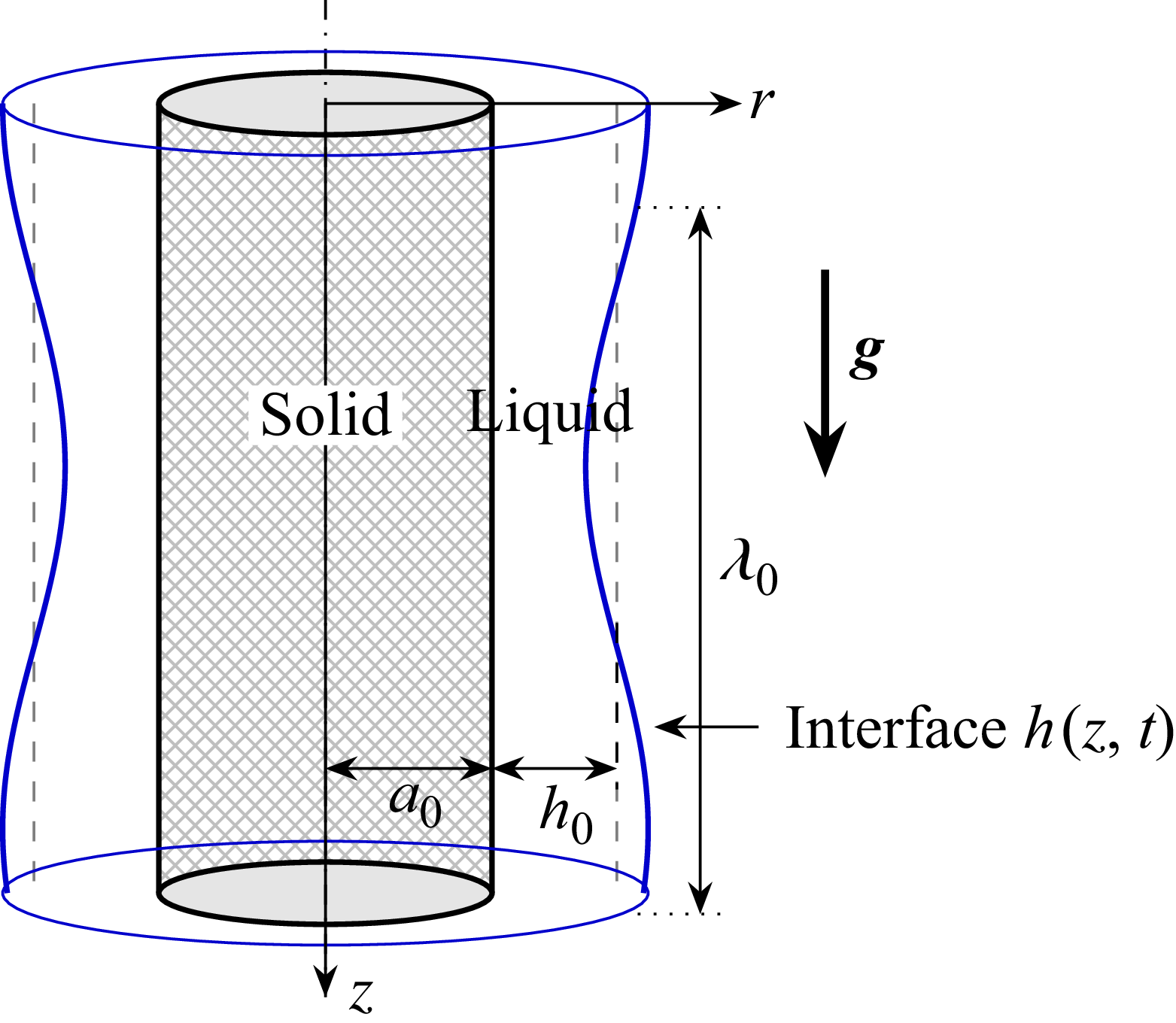
 a0
 h0
 g
 z
 h(z,t)
 λ0

 Ωi
 κ
 a
 Bo
 M
 Re=0.1
 ek
 τ^zz
 κc
 Bo
 a=0.3
 Re=0.1
 M=0.01
 M
 a=0.3
 Bo=0.3
 Re=0.1
 κc
 Ωi(κc)=0
 0<κ<κc

 a=0.3
 Bo=0.3
 M=0.1
 (κ,Ω)
 Ω0,i>0

 a=0.5
 Bo=0.5
 M=0.01
 (κ,Ω)
 Ωmax,i>0
 Ω0,i<0

 (Bo,a)
 M=0
 M=0.5
 Re=0.1
 Ω0,i
 Bo
 a=0.3
 M=0
 M=0.5
 Ω0,i

 M=0.01
 a
 Bo=0.3
 W=6
 (r,z)
 t=10
 t=50
 a=0.2
 a=0.4
 a=0.6
 r=±a
 h(z,t)
 a=0.2
 a=0.6

 M
 a=0.4
 Bo=0.3
 W=6
 (r,z)
 t=20
 t=50
 M=0
 M=0.1
 M=0.5
 M=0
 M=0.5
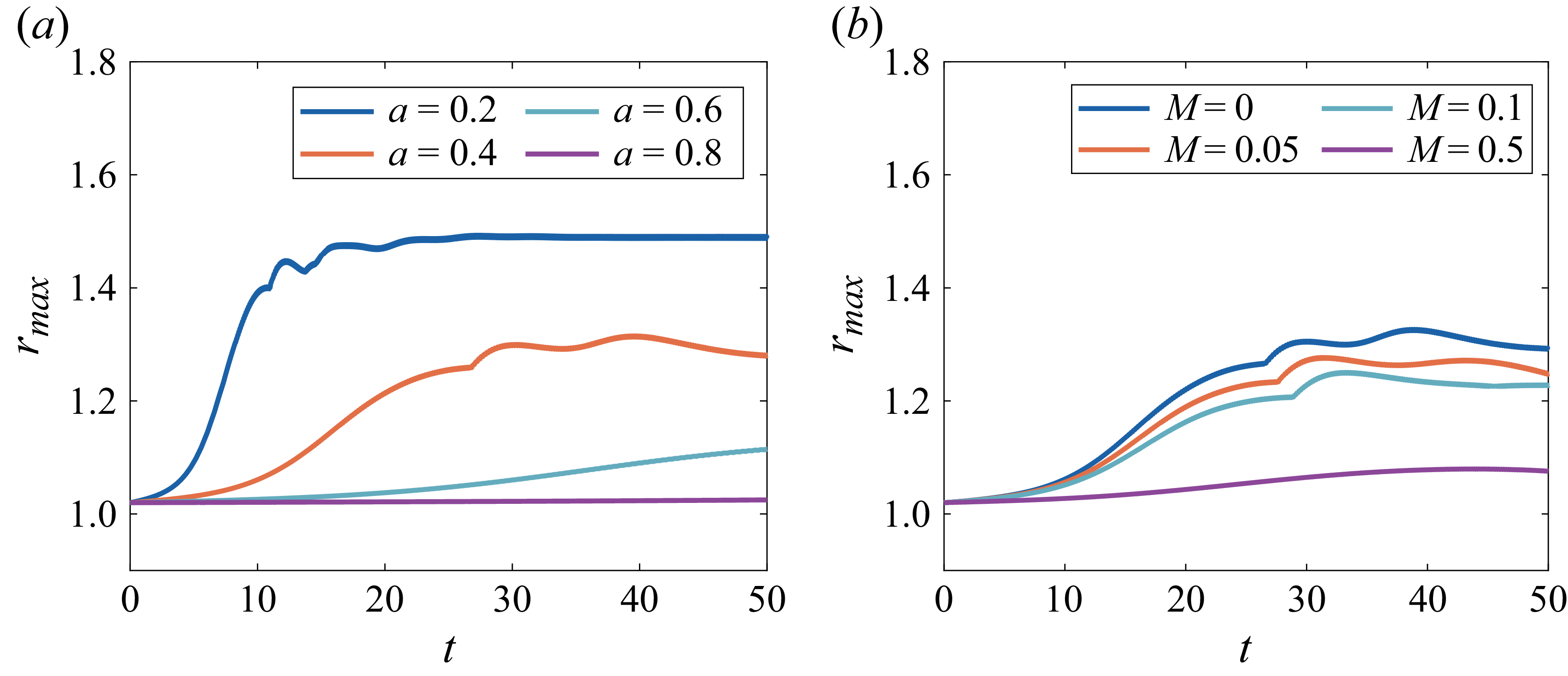
 rmax(t)
 a
 M=0.01
 Bo=0.3
 W=6
 M
 a=0.4
 Bo=0.3
 W=6
 M=0

 z0=10
 W=80
 Bo=0.2
 M=0.01
 (r,z)
 a=0.25
 t=10.38
 a=0.35
 t=30
 a=0.45
 t=30
 h(z,t)
 a=0.35
 Bo=0.2
 a=0.45
 Bo=0.2

 z0=10
 W=80
 Bo=0.2
 M=0.01
 hmin(t)
 a=0.25
 a⩾0.35
 |h~(z0,t)|
 a=0.25
 0.35
 a=0.45
 0.55

 a=0.2
 Bo=0.2
 W=50
 z0=10
 hmin≈0.05
 M=0
 t=7.05
 M=0.1
 t=7.12
 M=0.2
 t=6.58
 z
 h(z,t)
 M=0
 M=0.15

 W=50
 z0=10
 a=0.2
 Bo=0.2
 hmin(t)
 M
 tc
 hmin→0
 hmin
 tc−t
 hmin∼(tc−t)m
 m≈0.5

 W=50
 z0=10
 a=0.2
 Bo=0.2
 h(z,t)
 h/(tc−t)m
 (z−zc)/(tc−t)1/2
 M=0
 m=0.50
 M=0.2
 m=0.42

 a=0.2551
 c=1.21
 ε=0.2915
 W=5.81
 a=0.2856
 c=0.46
 ε=0.2330
 W=1.64
 a=0.3262
 c=1.37
 ε=0.178
 W=8.19
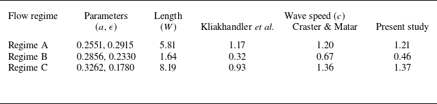
 c
 M=0

 M=0
 M=0.2
 a=0.2551
 ε=0.2915
 a=0.2856
 ε=0.2330
 a=0.3262
 ε=0.178

 (h,h′)
 M
 a=0.2551
 ε=0.2915
 a=0.2856
 ε=0.2330
 a=0.3262
 ε=0.178

 hmax
 c
 M
 a=0.2551
 ε=0.2915
 a=0.2856
 ε=0.2330
 a=0.3262
 ε=0.178


