


Introduction
Threats posed to the integrity and usefulness of research by publication bias are staple topics of discussions of statistical meta-analysis (e.g., Borenstein, et al., Reference Borenstein, Hedges, Higgins and Rothstein2009; Carter et al., Reference Carter, Schönbrodt, Gervais and Hilgard2019; Hedges, Reference Hedges1992; Rothstein et al., Reference Rothstein, Sutton and Borenstein2005) and of the apparently widespread difficulty of replicating statistically significant findings (Fidler & Wilcox, Reference Fidler and Wilcox2018). In such discussions the term publication bias has chiefly been used to refer to the tendency of publication gatekeepers (especially editors and reviewers) to approve submitted reports of statistically significant findings in preference to equally good reports of inconclusive findings. Discussions of publication bias frequently include discussion both of “file drawering” and a large category of questionable practices referred to as “p-hacking” (Head et al., Reference Head, Holman, Lanfear, Kahn and Jennions2015; Simonsohn et al., Reference Simonsohn, Nelson and Simmons2014a, Reference Simonsohn, Nelson and Simmons2014b, Reference Simonsohn, Simmons and Nelson2015, Reference Simonsohn, Nelson and Simmons2019), “hidden flexibility” (Chambers, Reference Chambers2017), or “selective reporting” (Head et al., Reference Head, Holman, Lanfear, Kahn and Jennions2015; Simonsohn et al., Reference Simonsohn, Nelson and Simmons2014a), among several other terms. File-drawering and p-hacking are both most likely to occur when researchers assume that publication bias exists and believe that their work has been or may be affected by it.
File drawering occurs when a researcher either makes no attempt to publish or else gives up attempting to publish a study or part of a study that yielded p > α for a result in the expected direction or that yielded a result of p > α or p < α in the unexpected direction. Because file-drawered studies tend to be ones that found relatively small effects, a consequence of file drawering is that findings of small effects remain disproportionately unavailable to other researchers and to meta-analysts. A result of this is that published estimates of effect sizes tend to be inflated, with potential adverse effects on theory and research agendas (e.g., Borenstein et al., Reference Borenstein, Hedges, Higgins and Rothstein2009; Hedges, Reference Hedges1992; Rosenthal, Reference Rosenthal1979; Rothstein et al., Reference Rothstein, Sutton and Borenstein2005).
The terms p-hacking, selective reporting, and so on denote types of biased selection among available options in data collection, data analysis, and reporting of results―or, more precisely, the “misreporting of true effect sizes in published studies [that] occurs when researchers try out several statistical analyses and/or data eligibility specifications and then selectively report those that produce significant results” (Head et al., Reference Head, Holman, Lanfear, Kahn and Jennions2015, p. 1). Because of its especially frequent use in the recent literature, the term used most often in this article is p-hacking. It is likely, though, that much p-hacking occurs not because researchers mean to cheat but because they hold mistaken beliefs about what analytic procedures are permissible (Gelman & Loken, Reference Gelman and Loken2013).
Wicherts et al. (Reference Wicherts, Veldkamp, Augusteijn, Bakker, van Aert, Robbie and van Assen2016) discussed 34 types of p-hacking, for example: (a) dealing with outliers in an ad hoc manner or, worse yet, dealing them only after finding p > α (hereafter α = .05), then retesting the data in the hope of finding p < .05, and, finally, reporting only the most favorable result (Bakker & Wicherts, Reference Bakker and Wicherts2014; Pollet & van der Meij, Reference Pollet and van der Meij2017); (b) failing to report tested dependent measures or covariates for which p > .05; and (c) carrying out two or more different tests of statistical significance on the same data (e.g., a t-test and a Wilcoxon–Mann–Whitney test [WMW]) and, if only one test yields p < .05, then reporting only that p-value.
Context, gradations, and incidence of p-hacking
Taking as background the evidently common situation in which researchers feel pressured for a study to yield at least one significant result, Gelman and Loken (Reference Gelman and Loken2013) described how a researcher engaged in a quantitative study must choose among options that arise at many separate stages, from conception to reporting. Within this state of affairs, vividly characterized by Gelman and Loken as “a garden of forking paths,” it is often easy for a researcher to make a sequence of decisions―each decision being defensible in itself but also arbitrary and motivated―that leads eventually to a statistically significant result in some part of the experimental design.Footnote 1 Indeed, the scope for hidden flexibility in decision making is typically so wide that, as demonstrated by Simmons et al. (Reference Simmons, Nelson and Simonsohn2011), researchers who engage in determined p-hacking in multiple seemingly tiny ways can succeed in finding p < .05 for almost any research hypothesis whatsoever. It is plausible that such a result is especially easy to achieve in a field such as SLA where research hypotheses typically have the potential to involve a multitude of variables of intersecting types (e.g., pedagogical, temporal, cultural, item-related, and learner-related) (cf., Roettger, Reference Roettger2019).
While it has been speculated that p-hacking in applied research tends to be modest in degree (Simonsohn et al., Reference Simonsohn, Simmons and Nelson2015), results of a survey carried out by John et al. (Reference John, Loewenstein and Prelec2012) indicate that p-hacking has been knowingly engaged in from time to time by an appreciable minority of researchers in psychology, an important feeder field of SLA. A particularly striking result of the survey of John and colleagues is that a sizeable proportion of the researchers who admitted to having engaged in types of p-hacking seemed to be unaware of the extent to which those practices are types of scientific misconduct that can degrade the quality of shared knowledge within their research community. To give an example of a different sort, Bakker and Wicherts (Reference Bakker and Wicherts2011) examined 281 randomly selected articles in high- and low-impact journals of psychology and found that about 18% of the reported p-values were inconsistent with the reported degrees of freedom and/or the test statistic. Bakker and Wicherts found additionally that erroneous p-values tended to be in a direction favorable to researchers’ hypotheses. One possibility then is that researchers, without necessarily being aware of it, are selective in how carefully they proofread their results sections.
The challenge of distinguishing signs of p-hacking from signs of file-drawering
There are at least a dozen methods for estimating and perhaps also correcting for the incidence of file-drawering in a body of related quantitative studies (e.g., Carter et al., Reference Carter, Schönbrodt, Gervais and Hilgard2019; van Aert & van Assen, Reference van Aert and van Assen2021).Footnote 2 Among the best known of these methods are “fail-safe N,” for estimating the number of effect sizes in the file-drawer (Rosenthal, Reference Rosenthal1979); “funnel plotting,” for detecting so-called small study effects (Egger et al., Reference Egger, Smith, Schneider and Minder1997; Light & Pillemer, Reference Light and Pillemer1984); “Egger’s regression test,” for testing funnel plot symmetry (Egger et al., Reference Egger, Smith, Schneider and Minder1997); and “trim and fill,” for correcting funnel plot asymmetry (Borenstein et al., Reference Borenstein, Hedges, Higgins and Rothstein2009; Duval & Tweedie, Reference Duval and Tweedie2000). In contrast, methods devised specifically to detect p-hacking have been lacking. For one thing, procedures conceived for the purpose of detecting file-drawering and/or compensating for it are unable to distinguish signs of p-hacking from signs of file-drawering. This is true, for instance, of methods commonly used by SLA meta-analysts. One example is trim and fill combined with funnel plotting.Footnote 3 Essentially, researchers using existing methods for detecting and mitigating impacts of file-drawering must assume that there was no p-hacking in the primary studies being investigated (e.g., Carter et al., Reference Carter, Schönbrodt, Gervais and Hilgard2019). Yet there is abundant evidence that p-hacking is a threat that must be taken seriously (e.g., Bakker & Wicherts, Reference Bakker and Wicherts2011; Simmons et al., Reference Simmons, Nelson and Simonsohn2011). In short, there is a need for a separate method that detects p-hacking. Fortunately, there is such a method. It is hoped that this article will accelerate its use by researchers of SLA.
Introducing p-curving
The present study introduces a comparatively simple and effective method―dubbed “p-curving” or “p-curve analysis” by Simonsohn et al. (Reference Simonsohn, Nelson and Simmons2014a)―that was developed specifically to detect signs of p-hacking. A salient feature of this method is that it is based entirely on a distribution of significant p-values. The prime rationale for this restriction is that a published statistically significant finding cannot have been affected by file drawering because being affected by file drawering means not being published. Consequently, any bias detectable in a set of significant p-values is likely to stem from p-hacking. A second rationale for the focus on significant p-values is that, for any given research hypothesis, it is comparatively easy to find a reasonably complete sample of studies that yielded a relevant significant p-value. In contrast, owing to file drawering, it is often impossible to be certain of having found even a majority of relevant studies where p > .05 (Hedges, Reference Hedges1992; Simonsohn et al., Reference Simonsohn, Nelson and Simmons2014a).
P-curves
Definitions
The term p-curve denotes a “distribution of statistically significant p-values for a set of independent findings” (Simonsohn et al., Reference Simonsohn, Nelson and Simmons2014a, p. 535), where “independent findings” are findings made in separate studies based on responses from different study participants. However, for extra clarity this article sometimes replaces the term p-curve with the longer expression 0 to .05 p-curve so that the expression 0 to 1 p-curve can be used to refer to a distribution of significant or nonsignificant p-values for a set of independent findings.
P-curves are important because inspection of a p-curve can reveal signs of p-hacking. This is possible because it is known what p-curves should look like in the absence of p-hacking. But what should any p-curve look like in any circumstance? The next section begins the process of answering that question.
A p-curve when the null hypothesis of no effect is true and there was no p-hacking
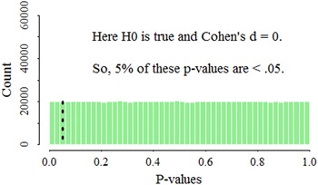
When a null hypothesis (H0) is true and a relevant test of statistical significance is unbiased, a vastly long sequence of properly conducted and properly analyzed studies independently addressing that H0 can normally be expected to yield a distribution of p-values that is either completely “uniform” (i.e., flat) or very nearly so (e.g., Head et al., Reference Head, Holman, Lanfear, Kahn and Jennions2015; Lakens, Reference Lakens2014; Simonsohn et al., Reference Simonsohn, Nelson and Simmons2014a).Footnote 4 In such a distribution, 5% of the p-values lie between 0 and .05; a further 5% lie between .05 and .10; and so on right up to and including the interval between .95 and 1, as indicated by Figure 1. (R script for all simulations and figures is given in the final section of the online Supplementary Materials and on the Open Science Framework at osf.io/vsqg8)
The distribution of p-values from Student’s independent samples t-test applied to one million pairs of samples, where each sample “X” and each sample “Y” (n X = n Y = 20) was a random draw from a normal distribution having Mn = 10 and SD = 1. Note: The dashed line marks p = .05.

Because the p-values shown in Figure 1 were derived by performing independent samples (IS) t-tests on samples drawn randomly from a single population in which the true effect size is 0, it was a matter of chance whether the mean of a sample X turned out to be greater than the mean of a sample Y or vice versa. The size of any particular mean difference was a matter of chance as well. Thus, every significant p-value represented in Figure 1 is significant solely because of random sampling variation. Hence, one useful interpretation of a flat 0 to .05 p-curve is that a study represented in that interval would fail to yield a significant p-value 19 times out of 20 if it was directly replicated with new learners.
A p-curve when the H0 of no effect is false and there was no p-hacking
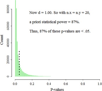
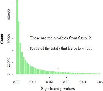
If the H0 is false (e.g., if True Mean X ≠ True Mean Y), then the distribution of p-values will show some degree of right-skew. In other words, most of the p-values will be heaped up near 0 with a thin tail of larger p-values extending to the right (Figure 2): Technically, the p-values will have an “exponential” distribution. When sample sizes are large (e.g., of size 200 rather than 20) and when the H0 is conspicuously false (e.g., when two population means are very different), then the right skew of a p-curve may reach the point of being essentially L-shaped, or even nearly columnar (e.g., Lakens, Reference Lakens2014). Importantly, this rightward skew of p-values will also be evident within the range 0 to .05 (Figure 3).
One million p-values generated in the same way as for Figure 1 except that Mn X = 10 and Mn Y = 11. Note: The dashed line marks p = .05.

The 0 to .05 portion of the p distribution depicted in Figure 2. The exponential distribution is still conspicuous. Note: The dotted line marks p = .025.

A p-curve when the H0 is true and there was p-hacking
Having considered the shape of p-curves when there was no p-hacking, we are ready to consider what p-curves may look like when p-hacking did occur. In the first of the following two simulated scenarios the built-in true effect was 0; however, concurrently two types of p-hacking were at play. One type was ad hoc exclusion of outliers. The other was an egregious version of the practice of applying two significance tests to the same data in the hope of increasing the chance of finding p < .05. Specifically, the simulation mimicked a scenario in which a researcher conducts a t-test on two independent samples using software that automatically supplements t-test results with results of the WMW test. In the scenario, the researcher chooses the t-test p-value if p < .05. But if that p value is > .05, the researcher chooses the p-value from the WMW test if it is < .05. But if neither test has yielded p < .05, the simulated researcher deletes the minimum and maximum values from each dataset and then tests the difference between the two trimmed datasets, choosing the p-value from the t-test if p < .05. But if that p-value is > .05, the researcher chooses the p-value from the WMW test whatever it happens to be. Further, the simulated researcher reports the chosen significance test without mentioning any of the others. The scenario was simulated one million times with the following settings: n X = n Y = 25; Mn X = Mn Y = 20; SD X = 4.50; SD Y = 4.00.
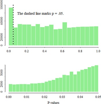
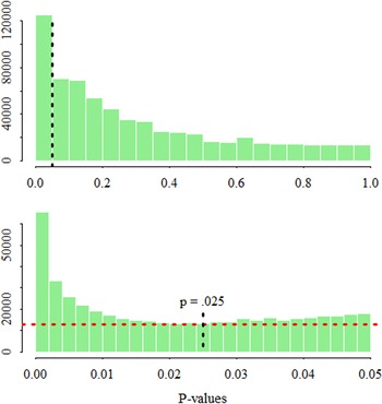
The p-curve resulting from the new simulation is depicted in Figure 4. In the upper histogram in that figure it can be seen that on average there are almost twice as many p-values in the 0↔.05 column, or “bin,” as in any of the other 19 bins. The excess p-values in the 0↔.05 bin represent type I errors (i.e., false findings). However, it is the lower histogram in Figure 4 that displays the clearest sign of p-hacking―namely, the distribution of statistically significant p-values is left skewed.
The combined effect of two types of p-hacking when d = 0.

A p-curve when the H0 is false and there was p-hacking
An additional simulation was carried out to illustrate p-hacking when there is a true effect that is large enough to be pedagogically significant. In this simulation the settings for the X and Y scores were as for the previous simulation except that now Mn X = 20 and Mn Y = 22. Thus, d population = 0.47. In both histograms in Figure 5 the existence of an appreciable effect is signalled by the disproportionately tall bins of p-values near 0. In the lower histogram, concurrent p-hacking is indicated by the fairly consistent left skew between about .02 and .05.
This display illustrates the combined impact of two types of p-hacking along with a true effect of moderate size. Notes: In the upper histogram the dotted line marks p = .05. The horizontal line in the lower histogram serves to underscore the concavity of the 0 to .05 p-curve.

Although a region of left skew in a 0 to .05 p-curve (as in the lower histogram in Figure 5) is a classic indicator of p-hacking, it is important to remain aware that the shape of a 0 to .05 p-curve is determined by multiple factors (Bishop & Thomas, Reference Bishop and Thompson2016; Gelman, Reference Gelman2018; Hartgerink, Reference Hartgerink2017; Lakens, Reference Lakens2014). Among these factors, the size of the true effect is likely to be especially important. Factors that tend to be of lesser importance include the type(s) of statistical significance test used in the underlying primary studies (e.g., Welch’s IS t-test vs. Student’s IS t-test) and the type of raw data in those studies (e.g., continuous vs. discrete). Also important are the sizes of the samples in the underlying primary studies and the stability of the true effect from context to context. The comparative importance of p-hacking depends on the incidence of p-hacking and the type(s) of p-hacking involved. Also, each of the p-curves illustrated in this article so far was based on one million p-values. Consequently, the outlines of these p-curves would remain essentially stable if the simulations were repeated with different sequences of random numbers. However, in practical research p-curves will be based on far fewer p-values, meaning that the contour of any given p-curve may be strongly influenced by random sampling variation. The point being made here is that interpretation of real world p-curves calls for caution.
It is relevant that left skew can result not only from p-hacking but also from an apparently small number of inadvisable practices that have nothing to do with trying to change p > .05 into p < .05. Erdfelder and Heck (Reference Erdfelder and Heck2019) considered a scenario in which a researcher uses ANCOVA and finds p < .05. But the researcher goes on to use ANOVA or a t-test also, because compared to ANCOVA these procedures are better known, they require fewer assumptions, and they can be described in comparatively few words. Finally, if the ANOVA (or the t-test) yields p < .05 then, for simplicity and brevity, the researcher reports this p-value without mentioning the use of ANCOVA. If this scenario occurred in an appreciable proportion of the primary studies underlying a p-curve, that curve might show some left skew simply because a significant p-value from an ANOVA or a t-test will often be larger than a corresponding ANCOVA p-value. It may be doubted though that this scenario is at all common in SLA research.
Uses of p-curving with respect to the possible presence of p-hacking
Although p-curving can have a second use that is touched on in a later section, this article focuses on its use to gain an impression of the overall trustworthiness and replicability of a set of published statistically significant results. There are several types of situation in which SLA quantitative researchers should consider p-curving for the purpose just mentioned, given that existence of p-hacking is a realistic possibility.
First, p-curving can enhance the planning of a research program. For example, Lakens (Reference Lakens2018) demonstrated how p-curving can enable a researcher to distinguish between a research path that is promising and one that is not. In Lakens’s study, each path had to do with a behavioral effect of priming, but the types of priming were not the same. Both types had been experimentally studied multiple times, and for each type statistically significant positive results had been published. For each of these two sets of published results Lakens constructed a 0 to .05 p-curve. He found that one of the p-curves was strongly indicative of p-hacking whereas the other showed the hallmark of solid evidential value―namely, conspicuous right skew. Lakens’s point was that p-curving can make the difference between embarking on program of successful research and embarking on a research program that leads a succession of results that are inconclusive and unpublishable.
A second use of p-curving is exemplified by a very large-scale, multisite study carried out by Dick et al. (Reference Dick, Garcia, Pruden, Thompson, Hawes, Sutherland, Riedel, Laird and Gonzalez2019) to address the hypothesis that childhood SLA is beneficial to development of (cognitive) executive function. Past results regarding this hypothesis had been mixed. Dick et al. subjected the relevant statistically significant p-values to a p-curve analysis and found little sign of a substantively significant true effect when possible effects of p-hacking were taken into account. Dick et al. used this result as one component of their tripartite basis for stating that their study revealed no persuasive evidence of a bilingual advantage for executive function in children aged from 9 to 10.
Simonsohn et al. (Reference Simonsohn, Nelson and Simmons2014a, p. 535) suggested a range of additional uses of p-curving, as follows. First, p-curving “will be useful to anyone who finds it useful to know whether a given set of significant findings is merely the result of selective reporting.” Second, p-curving may help researchers to “decide which articles or literatures to read attentively, or as a way to assess which set of contradictory findings is more likely to be correct.” Third, a p-curve analysis may suggest an explanation of inconsistencies between one’s own findings and findings published previously. Fourth, “reviewers may use p-curve [sic] to decide whether to ask authors to attempt a direct replication prior to accepting a manuscript for publication.” Fifth, reviewers and editors may conduct p-curve analyses to gain an impression of the reliability of findings relating to a research hypothesis addressed in a submitted research report. Simonsohn et al. suggested additionally that p-curving might be applied to a single article that reports many p-values. However, discussion of this last use is beyond the scope of this article. Finally, p-curving is a tool for assessing the evidential value of statistically significant findings in a stream of research covered by one or more published quantitative meta-analyses or narrative literature reviews. A later section of this article presents a case study of p-curving with respect to two published quantitative meta-analyses.
The assumption of homogeneity in p-curving
Developers of the p-curve method for detecting p-hacking have stressed that it works best when an effect of interest is relatively homogeneous at population level; and they have pointed out that problems of interpretation arise if the magnitude of an effect varies notably from context to context (Simonsohn et al., Reference Simonsohn, Nelson and Simmons2014a). However, in applied research the degree to which an effect is homogeneous at population level is generally unknowable. Accordingly, a prospective p-curver will need to make an informed judgement about the homogeneity (vs. heterogeneity) of the effect of interest before undertaking a p-curve analysis. That said, many useful statistical procedures depend on the ultimately unverifiable tenability of assumptions about population characteristics: ANOVA is a prime example.
The homogeneity or heterogeneity of studied effects has been a major concern in recent studies of p-curving for the purpose of estimating true effect sizes (e.g., McShane et al., Reference McShane, Böckenholt and Hansen2016). The consensus seems to be that p-curve methods for this purpose must be adapted so that they take account of both significant and nonsignificant p-values because otherwise the resulting estimates are likely to be inaccurate and probably inflated whenever the true effects are heterogeneous (Carter et al., Reference Carter, Schönbrodt, Gervais and Hilgard2019; McShane et al., Reference McShane, Böckenholt and Hansen2016; van Aert & van Assen, Reference van Aert and van Assen2021).Footnote 5 It seems that no such adjustment is necessary or even feasible with respect to the p-curve method for detecting p-hacking.
Preparatory steps of p-curving using the online p-curve app
First steps of p-curving include choosing a research hypothesis and identifying a set of studies relating to that hypothesis. Then it is necessary to find the studies that yielded a directly relevant significant p-value―typically just one p-value per study. (An important exception is specified in the following text.) Note that in p-curving there is no averaging of related p-values analogous to the standard meta-analytic practice of averaging related effect sizes. Note too that if one’s working hypothesis happens to be that a true effect is positive, it is necessary to set aside any significant p-values that correspond to a negative effect. The opposite would be done if a negative effect has been hypothesized. Finally, it can be difficult and perhaps impossible to interpret a p-curve that includes p-values relating to different research hypotheses (e.g., Simonsohn et al., Reference Simonsohn, Nelson and Simmons2014a).
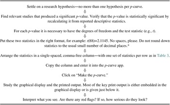
It is possible to create an informative p-curve histogram by using reported p-values. However, reported p-values are likely to be rounded to two decimal places, and some may be reported as, say, “< .05” or “< .001.” P-values that are desirably exact can usually be recalculated from reported descriptive statistics. Also, recalculation of p-values occasionally enables a reporting error to be corrected. However, there is a free-to-use “p-curve app” that produces superior print and graphical output and is supported by copious explanatory material (Simonsohn et al., Reference Simonsohn, Simmons and Nelson2015, Reference Simonsohn, Nelson and Simmons2017) (http://p-curve.com/). Use of this app does not require recalculation of p-values because these are calculated by the app. Throughout the rest of this article use of this app will be assumed. The essential steps of p-curving with the p-curve app are summarized in Table 1.
The basic steps of p-curving

* Further examples of correctly formatted sets of statistics are as follows: F(1,100)=.2460, f(2,2102)=4.4573, Z=3.45706, chi2(1)=9.1255
Because ANOVA has been so heavily used by SLA researchers (Lindstromberg, Reference Lindstromberg2016; Plonsky, Reference Plonsky2013; Plonsky & Gass, Reference Plonsky and Gass2011), it is important for p-curvers to bear it in mind that an attenuating interaction (in which an effect merely varies between being strong and weak) must be handled differently than a more radical reversing (or crossover) interaction. In the case of an attenuating interaction, the only p-value that is used is the one for the interaction. If an interaction is reversing, the p-curver uses the p-values for the simple effects (NB: not the main effects).
For an attenuating interaction the rationale is as follows:
When a researcher investigates the attenuation of an effect, the interaction term will tend to have a larger p value than the simple effect (because the latter is tested against a null of 0 with no noise, and the former is tested against another parameter estimated with noise). Because publication [bias] incentivizes the interaction to be significant, p values for the simple effect will usually have to be much smaller than .05 in order for the study to be published. This means that, for the simple effect, even p values below .05 will be censored [i.e., absent] from the published record and, thus, not uniformly distributed under the null [hypothesis]. (Simonsohn et al., Reference Simonsohn, Nelson and Simmons2014a, p. 543, note 16)Footnote 6
Finally, Simonsohn et al. (Reference Simonsohn, Nelson and Simmons2014a, p. 544) stated that 10 p-values can be the basis of an informative p-curve analysis, given adequate statistical power. However, their statistical power simulations assumed only 20 participants per group. (Coincidentally, 20 learners per group has been typical of between-subjects designs in SLA experimental research [Lindstromberg, Reference Lindstromberg2016; Plonsky, Reference Plonsky2013].) Recall, though, that for any given effect size, statistical power will rise with the number of participants per group, all else being equal. It is therefore plausible that somewhat fewer than 10 studies may suffice if the average group size in the studies is considerably larger than 20.
Guidelines for upholding the integrity of p-curve analyses
Various sets of guidelines have been proposed for maximizing the integrity of p-curve analyses (e.g., BITSS, 2017; Head et al., 2017; Simonsohn et al., Reference Simonsohn, Nelson and Simmons2014b, p. 1151). Two guidelines are particularly prominent in this literature. First, decide in advance which studies to include. Disclose the decision. Adhere to it. Second, be open about choices made in cases of uncertainty. For example, if it is unclear whether a study should be included in an analysis, report results for when the study is included and for when it is not. Fulfillment of these and other published guidelines are illustrated in and in connection with the case study that is reported in the text that follows.
P-curving in SLA and bilingualism research so far
To date p-curving has been little used or referred to either by SLA researchers or by researchers of bilingualism. In bilingualism research a conspicuous exception is the study by Dick et al. (Reference Dick, Garcia, Pruden, Thompson, Hawes, Sutherland, Riedel, Laird and Gonzalez2019) that was summarized in a previous section. Also with respect to bilingualism research, Plonsky et al. (Reference Plonsky, Sudina and Hu2021) referred to use of p-curving for the purpose of estimating effect sizes in a meta-analytic context. As to SLA research, Vitta and Al-Hoorie (Reference Vitta and Al-Hoorie2020) used the p-curve app (Simonsohn et al., Reference Simonsohn, Nelson and Simmons2017) to carry out a p-curve analysis as one strand of their standard random effects meta-analysis of empirical studies of the “flipped classroom.” Discussion of that p-curve analysis is postponed until after presentation of the case study illustrating an application of p-curve analysis.
A p-curving case study: L2 vocabulary glossing
Introduction
Fixed effects and random effects meta-analyses are unable detect p-hacking; and, as mentioned, the same is true of ancillary methods such as trim and fill (e.g., Carter et al., Reference Carter, Schönbrodt, Gervais and Hilgard2019; Simonsohn et al., Reference Simonsohn, Nelson and Simmons2014b; van Assen et al., Reference van Assen, van Aert and Wicherts2015; van Aert & van Assen, Reference van Aert and van Assen2021). Accordingly, it has been recommended that journals should publish p–curve reevaluations of the extent of p-hacking in sets of studies covered by published meta-analyses that included no effective checks for signs of p-hacking (van Aert et al., Reference van Aert, Wicherts and van Assen2019). The case study reported in the following text is intended to illustrate this use of p-curving in an SLA context. The case study covers primary studies that addressed the possibility that L1 and L2 glosses differ in the degree to which they promote acquisition of word meanings by learners of elementary or intermediate proficiency. In all these studies learners were asked to demonstrate knowledge of what meaning attaches to a given L2 orthographic form in an immediate or near immediate posttest and, usually, in a delayed posttest as well. Although all the relevant primary studies used two-sided significance tests (α = .05), it seems likely that researchers generally expected to find that L1 glossing is comparatively effective. The case study proceeded from the assumption that the researchers did have this expectation.
The decision to build a case study around the previously mentioned research hypothesis was influenced by the following facts. First, vocabulary acquisition is an essential component of SLA. Second, two recent, relevant meta-analyses were available: Kim et al. (Reference Kim, Lee and Lee2020) and Yanagisawa et al. (Reference Yanagisawa, Webb and Uchihara2020). Third, these two meta-analyses covered enough acceptable primary studies for p-curving to be feasible and informative. Fourth, casual inspection of a large proportion of the primary studies cited by Kim et al. (Reference Kim, Lee and Lee2020) indicated that all necessary descriptive statistics were likely to be findable.
Importantly, all the candidate primary studies implemented one or more measures to reduce the chance that target words would be known to learners prior to the experimental treatment. These measure were staging a pilot study to vet candidate target words, administering a pretest either to screen out familiar candidate words or to screen out overly proficient learners, and using English-like pseudowords as targets. Thus, even for the studies that had not used random assignment of learners to treatment groups, it was reasonable to follow the original researchers in analyzing only the posttest scores―considering that the chief purpose of this case study is to demonstrate an application of p-curving rather than to illustrate ideal experimental design.
Constraints that the two meta-analyses imposed on the selection of primary studies
Prior to finalizing the list of to-be-included primary studies, it was decided that the p-curve analysis would include no studies other than the ones covered by Kim et al. (Reference Kim, Lee and Lee2020) and Yanagisawa et al. (Reference Yanagisawa, Webb and Uchihara2020). It was envisaged that this inclusion rule could serve as a transparent way to keep the case study from growing much larger than is necessary to illustrate an application of p-curving. It should be emphasized, though, that in the majority of practical applications it would be preferable for a p-curve analysis to include all relevant published studies findable anywhere.
This case study’s coverage of primary studies was indirectly limited by the decision of Kim et al. (Reference Kim, Lee and Lee2020) and Yanagisawa et al (Reference Yanagisawa, Webb and Uchihara2020) to exclude studies that were not reported in English and that did not use English as the target L2. Of the various other limitations on coverage which this case study inherited from Kim et al. and Yanagisawa et al., only one is questionable. Namely, Kim et al. excluded quasi-experimental studies that had not included use of a test of statistical significance test (generally one-way ANOVA) to confirm that treatment groups were equivalent prior to the treatment. A potentially serious drawback of this policy is that it excludes all primary studies carried out by researchers who know that this sort of baseline equivalence testing is ineffective and potentially misleading (Lindstromberg, Reference Lindstromberg2016; Norris, Reference Norris2015). Valid equivalence testing works very differently (e.g., Lakens et al., Reference Lakens, Scheel and Isager2018).
Choices determining study selection
In line with previously mentioned purposes and limitations of p-curving the following choices were made:
First, the case study would include only primary studies having an experimental design yielding score sets that can in principle be compared by using a two-sided IS t-test. This was partly because of the comparative scarcity of relevant primary studies having a within-subjects design (Yanagisawa et al., Reference Yanagisawa, Webb and Uchihara2020)―that is, a design in which all subjects experience all conditions―and partly because it is not straightforward to equate results stemming from such a design with results from a between-subjects design (e.g., Plonsky & Oswald, Reference Plonsky and Oswald2014). In particular, a p-value from a specific application of the paired t-test can relate to several different versions of d, each with its own value (Westfall, Reference Westfall2016). Second, the acceptance of a study was conditional on the availability of the relevant sample sizes, means, and SDs. Third, each study must have included at least one group of learners described as being mostly at elementary, low-intermediate, or intermediate level. This limitation was due to the unresolved matter of whether the positive effect of L1 glossing is appreciably attenuated in the case of highly proficient L2 learners.Footnote 7 Two exclusions were made solely because some or all test scores were described as having come from postintermediate learners. Fourth, because the relevant goal of p-curving is detection of p-hacking and because p-hacking is presumed to be a consequence of publication bias, it followed that the case study would only include studies reported in a named print or online journal.
Table A of the Supplementary Materials provides an overview of the 10 primary studies that survived the selection process plus an additional study (Kazerouni & Rassaei, Reference Kazerouni and Rassaei2016) that was not included in the meta-analyses of Kim et al. (Reference Kim, Lee and Lee2020) and Yanagisawa et al. (Reference Yanagisawa, Webb and Uchihara2020). Although apparently acceptable overall, Kazerouni and Rassaei’s study included neither random assignment of learners to groups nor BE testing. For these reasons that study would not have been eligible for inclusion in the meta-analysis of Kim et al. Kazerouni and Rassaei’s study is touched on again further in the text that follows. Finally, Table B in the Supplementary Materials lists candidate primary studies that were excluded from the present case study and gives reasons for their exclusion.
Selection of comparisons within primary studies
In many of the primary studies the variable gloss language (L1 vs. L2) was crossed with another binary variable: gloss type (single word vs. multiple choice), learning mode (intentional vs. incidental), proficiency (low vs. high), or +/–picture.
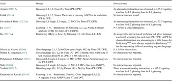
As there seems to be no persuasive evidence that gloss type appreciably moderates the effect of gloss language (Kim et al., Reference Kim, Lee and Lee2020; Yanagisawa et al., Reference Yanagisawa, Webb and Uchihara2020), the test scores for single word and multiple choice glossing were combined for each gloss language. For much the same reason test scores for the intentional and the incidental learning conditions were also combined for each gloss language. It seems relevant that two of the primary studies directly addressed the relative effects of intentional and incidental learning (see Table 2) but found p > .05. Further, +/–intentional learning is often operationalized as +/–forewarning-of-a-test, yet it cannot be taken for granted that most learners will assume that lack of forewarning is a sure sign that no test will follow (e.g., Barcroft, Reference Barcroft2015; Boers, in press). Finally, while six studies definitely did not include forewarning, for two studies it was not made clear whether there was forewarning or not.
Experimental designs of the p-curved primary studies

a PT = (near) immediate posttest; DPT = delayed posttest.
b MC = multiple choice glossing.
c This extra study is discussed in a later section of this article.
A different policy was adopted regarding proficiency and +/–picture, on the assumption that it is comparatively risky to assume that these variables do not appreciably moderate the effect of gloss language. Specifically, when a primary study explicitly distinguished between high- and low-proficiency learners, the case study used only the test scores from the low-proficiency group; and when a study had +picture and –picture conditions (i.e., Yoshii, Reference Yoshii2006), the case study used only the scores for the –picture condition. Lastly, with respect to proficiency, Kim et al. (Reference Kim, Lee and Lee2020) applied the term beginner to the learners in a large fraction of the primary studies figuring in the present case study. By my reading of the corresponding original articles, the labels elementary, postbeginner, or preintermediate seem more apt, depending on the study.
The policy regarding interactions
All the candidate primary studies had a between-groups design at each time of testing. However, most of the studies included a delayed posttest, meaning that there could be within-subjects testing of retention (or forgetting). Some of the studies detected an attenuating interaction involving time. Specifically, less forgetting was associated with L2 glossing than with L1 glossing despite overall superiority of L1 glossing. For these studies the relevant p-value was the p-value for the interaction between time and gloss language (see Table 2). Further, Ko (Reference Ko2017) observed an attenuating interaction between proficiency and gloss language at the immediate posttest. The interaction p-value was used for that study also.
Calculating the necessary statistics for p-curving
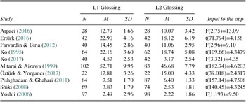
The function tsum.test in the R package BSDA (Arnholt, Reference Arnholt2017) was used to expedite calculation of t-statistics, degrees of freedom, and p-values. This function applies Welch’s t-test, which uses degrees of freedom that may run to several decimal places. Once computed, the key statistics for each study were formatted as described in Table 1 and as shown in the far right column of Table 3.
The p-curve analysis: Studies and statistics*

* Some authors gave descriptive statistics to more decimal places than are shown here: Recalculation of degrees of freedom and t-statistics was based on the descriptive statistics as authors reported them.
Results of the main p-curve analysis and what they mean
A key item in the copious output of the p-curve app of Simonsohn et al. (Reference Simonsohn, Nelson and Simmons2017) is a 0 to .05 p-curve graph to be discussed in a later paragraph. Related to that graph are six tests of statistical significance able to furnish evidence that a p-curve reflects a practically significant level of evidential value over and above any distortion by p-hacking. The app presents the six significance tests in groups of three. The first group of tests are one-sided tests of the H0 that the p-curve has a flat or left-skewed distribution. For these tests p < .05 indicates right skew, which in turn indicates appreciable overall evidential value.
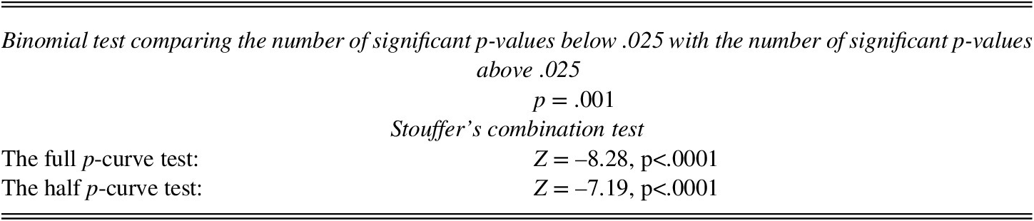
The results from the first three tests are given in Table 4. The binomial test addresses the H0 that there are as many significant p-values above .025 as there are below .025. The directional alternative hypothesis is that most of the p-values lie below .025. Because this test gave p < .05, it is warranted to conclude that the p-curve (Figure 6) shows evidential value. However, the binomial test is based on values dichotomized as either 1 (for < .025) or as 0 (for > .025). Consequently, this test may lack statistical power to detect moderate right skew. Tests two and three in Table 3 are applications of Stouffer’s combination test. This test is based on p-values that have been transformed but not dichotomized. An application of Stouffer’s test can therefore be expected to have more power than a corresponding application of the binomial test. A sufficiently large Z score from Stouffer’s test signifies a high proportion of small p-values (i.e., right skew) in the range at issue. The first Stouffer’s test focuses on the 0 to .025 half p-curve. Any left skew between 0 and .025 would suggest very drastic p-hacking. The second Stouffer’s test focuses on the whole 0 to .05 p-curve. This test is intended to be comparatively sensitive to moderate p-hacking. Table 4 shows that each Stouffer’s test rejects its H0.
Results of three statistical significance tests of the null hypothesis is that there is no right skew in the p-curve shown in Figure 6

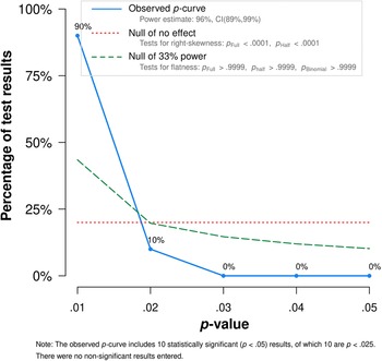
P-curve produced by the online app of Simonsohn et al. (Reference Simonsohn, Nelson and Simmons2017).

The results given in Table 4 indicate that the 10 focal primary studies have overall evidential value with respect to the research hypothesis addressed by this case study. But approximately how much evidential value? This question brings us to Figure 6, which shows the graph produced by the p-curve app. In discussing Figure 6 let us begin with the dotted horizontal line near the bottom of the graph. This line depicts the p-curve that would be expected if L1 and L2 glossing have the same effect on L2 vocabulary learning. In Figure 6 it can be seen that the observed p-curve, represented by the solid line, deviates from the dotted line dramatically. The label “90%” by the left end of the solid line indicates that 9 of the 10 p-values are < .01. This percentage is consistent with the 10 primary studies having considerable evidential value. More exactly, the extreme heaping of p-values near 0 reflects some combination of adequate sample sizes in the primary studies and an appreciable true difference between the effect of L1 glossing and the effect of L2 glossing for learners ranging approximately from elementary to intermediate in proficiency.
Still focusing on Figure 6 we now come to the dashed curve, which becomes relevant if the observed p-curve has minimal right skew. This dashed curve represents the approximate minimum of right skew consistent with substantively, or pedagogically, significant evidential value. The corresponding significance tests (i.e., tests 4 to 6) are, respectively, a binomial test and two Stouffer’s tests. If they show p > .05, it is warranted to conclude that the observed p-curve represents a modicum of evidential value. For the p-curve shown in Figure 6, these three tests give p > .999. If they had yielded p < .05, that would have indicated either the likely absence of a pedagogically significant true effect or an insufficient level of statistical power to detect whatever true effect may be present. Lack of power could be corrected by finding additional relevant primary studies. It would be an especially bad sign if the left end of the solid line remains below the dashed line. Conversely, p-hacking would be fairly dramatically indicated if the right end of the solid line rises above the dashed line. Technical details about the p-curve app and its output are available both at http://www.p-curve.com/ and in material that accompanies a computed p-curve graph.
Finally, the small print at the top of Figure 6 gives 96% as the estimate of the average “observed,” or post hoc, statistical power of the 10 studies underlying the p-curve. In most research situations observed power, unlike a priori power, is of little or no interest for reasons set out by Lakens (Reference Lakens2021). The textual output of the p-curve app explains the special role of observed power with respect to the app’s graphical output.
A further step in p-curve analysis: Checking robustness
At this point in a p-curve analysis, an important question remains: Is the observed p-curve overly dependent on outliers―that is, on primary studies that yielded extremely low or extremely high significant p-values? This question can be answered by deleting p-values at either extreme of an observed p-curve to see how the curve changes. Technically, a type of “robustness test” is called for. Here again the p-curve app employs Stouffer’s test. In the app’s robustness testing, one implementation of Stouffer’s test focuses on the observed 0↔.05 p-curve. In the present case that test continued to yield p < .05 at every stage of the value-by-value cumulative omission of the four lowest p-values. A second robustness test continued to yield p < .05 when the procedure was repeated, but this time working from the highest p-value downward. A third robustness test focusing on the 0↔.025 half-curve consistently yielded p < .05 when working from the lowest p-value up. It can therefore be concluded that the 10 studies involved in the p-curve analysis have robust evidential value.
Discussion
From the results given in Table 4 and from the shape of the p-curve shown in Figure 6 it is inferable, first, that the 10 primary studies covered by the main p-curve analysis have notable evidential value. It is inferable also that there was no worrying p-hacking, there being no p-values between .02 and .05. Moreover, the results of the robustness tests are reassuring. All this matters and is encouraging because the effect sizes corresponding to the 10 underlying p-values will have made a prominent contribution to the estimate of average effect size that Kim et al. (Reference Kim, Lee and Lee2020) reported for the research hypothesis at issue in this case study. However, the proportional contribution of present results must be smaller with respect to the estimate of Yanagisawa et al. (Reference Yanagisawa, Webb and Uchihara2020) because that meta-analysis focused on studies of incidental learning and because it included many unpublished studies not covered by this case study.
Although the previously mentioned results of the p-curve analysis are encouraging, it should be borne in mind that p-curve analysis is not a tool for assessing overall study quality: Studies should be vetted for quality before p-curving begins. To say more about quality, recall that 4 of the 10 primary studies figuring in this case study were quasi-experimental. It is not controversial to say that results from quasi-experiments tend to be less credible than results from experiments. It is noteworthy also that each of the 10 primary studies generated raw test scores that were binary (i.e., correct or incorrect) for each target vocabulary item and that all of the researchers used ANOVA and/or t-tests for which the binary scores were subtotaled by learner. It is now widely recognized that it is usually preferable to analyze binary vocabulary test scores by using mixed-effects logistic regression (Linck & Cunnings, Reference Linck and Cunnings2015). See Boers (in press) for insightful discussion of the quality of published studies of the effects of glossing on L2 vocabulary learning.
Lastly, in an earlier section it was mentioned that Simonsohn et al. (Reference Simonsohn, Nelson and Simmons2014a) suggested 10 as the minimum number of primary studies needed for a useful p-curve if statistical power is adequate (Simonsohn et al., Reference Simonsohn, Nelson and Simmons2014a). It was mentioned too that Simonsohn et al. based their estimate on a mean sample size of 20 participants. The primary studies covered by the present case study had a median sample size of 52 participants (i.e., learners). Consequently, it is likely that 10 studies were indeed sufficient for this study. Still, it would have been preferable to have had p-values from additional studies. The aforementioned study by Kazerouni and Rassaei (Reference Kazerouni and Rassaei2016) was not included in the present p-curve analysis because it did not meet the main criterion of the preset inclusion rule, namely, coverage by Kim et al. (Reference Kim, Lee and Lee2020) or Yanagisawa et al. (Reference Yanagisawa, Webb and Uchihara2020). However, application of Welch’s t-test to Kazerouni and Rassaei’s immediate posttest scores produced t = 5.8437, df = 77.156, p = .0000001. This result is consistent with L1 glossing being comparatively effective for lowish proficiency learners like those in Kazerouni and Rassaei’s study. Interested readers may extend the 10-study p-curve analysis by adding t(77.156)=5.8437 to the list of statistics given in Table 3 and then submitting the extended list to the p-curve app (http://www.p-curve.com).
Two alternative strategies in p-curving
Until relatively recently quantitative researchers of SLA have relied extremely heavily on a small number of inferential analytic procedures, especially ANOVA, two-sample t-tests, and two-sample rank-based tests such as the WMW test (Lindstromberg, Reference Lindstromberg2016; Plonsky, Reference Plonsky2013; Plonsky & Gass, Reference Plonsky and Gass2011). With respect to these procedures, the statistical significance tests implemented by the p-curve app are able to warrant the conclusion that a p-curve reflects appreciable evidential value even when a minority of the p-values happen to reflect p-hacking―including some bold p-hacking. However, it was asserted by Head et al. (Reference Head, Holman, Lanfear, Kahn and Jennions2015) that the app’s significance tests may lack sensitivity to the presence of modest p-hacking, even though modest p-hacking is presumably more common than bold p-hacking. Head et al. stated in particular that the approach taken by the p-curve app can result in signs of modest p-hacking being masked when a strong average true effect results in dramatic heaping of p-values near zero. As a means of detecting modest p-hacking in this circumstance Head et al. recommended use of a one-sided sign test (a version of the binomial test). For this test the H0 would be that a specified segment of a p-curve is either right skewed or uniform. So, p < .05 would indicate left skew. The sign test could, for example, focus on the range .02↔.05 by comparing the number of p-values in the subrange .02↔.035 with the number in the subrange .035↔.05. Obviously, running such a test would only make sense if there were enough p-values in the full range of interest.
If the recommendation of Head et al. (Reference Head, Holman, Lanfear, Kahn and Jennions2015) is not applicable due to a dearth of relevant p-values, a practical alternative is suggested by best practice in attempting to understand a correlation. That is, interpretation should not cease with consideration of the correlation coefficient and perhaps of the associated p-value as well. Rather, it is always advisable to examine the corresponding scatterplot. This is the lesson afforded by “Anscombe’s quartet” (Anscombe, Reference Anscombe1973). Similarly, p-curvers should not place so much weight on the results of significance tests (e.g., the ones carried out by the p-curve app) that they overlook clues visibly afforded by the relevant p-curve graph. The next section deals with a case in point.
An authentic p-curve showing right skew and left skew
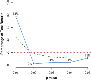
It may now be instructive to compare the p-curve shown in Figure 6 with the one shown in Figure 7. The latter is a simplified but essentially accurate rendering of a p-curve graph from the p-curve app that was displayed by Vitta and Al-Hoorie (Reference Vitta and Al-Hoorie2020) in relation to their meta-analytic review of studies having to do with “the flipped classroom” in SLA. This new p-curve graph is presented here to illustrate certain issues that may arise when a p-curve is to be interpreted.
The key elements of the p-curve presented by Vitta and Al-Hoorie (Reference Vitta and Al-Hoorie2020).

Two key facts regarding Figure 7 are as follows. First, this figure is based on all 45 of the significant p-values from Vitta and Al-Hoorie’s (Reference Vitta and Al-Hoorie2020) total sample of primary studies (k = 56). Second, those studies addressed at least three research hypotheses. A consequence of this last fact is that Figure 7 resists interpretation because it does not show which p-values in the curve relate to which research hypothesis. To resolve the unclarity it would be necessary to construct a separate p-curve for each research hypothesis (Simonsohn et al., Reference Simonsohn, Nelson and Simmons2014a). A second problem is that Vitta and Al-Hoorie made it clear that observed effects of flipped instruction have been heterogeneous with respect to each of the research hypotheses that they took into account. But, as mentioned in an earlier section of this article, it can be difficult to interpret a 0↔.05 p-curve when the underlying effects are heterogeneous.
A third issue regarding Figure 7 has to do with the information it would have conveyed (a) if all the underlying studies had addressed a single research hypothesis and (b) if it were reasonable to assume that the relevant observed effects correspond to an approximately homogeneous population effect. Given these two conditions, the significance tests which the p-curve app carried out on Vitta and Al-Hoorie’s (Reference Vitta and Al-Hoorie2020) data will indeed have indicated that the underlying p-values have considerable evidential value. This is inferable from the version of Figure 7 given in Vitta and Al-Hoorie’s article and from the associated commentary. Note in particular that Figure 7 shows that 78% of the underlying p-values are below .01. Nevertheless, their p-curve is skewed left between .02 and .05. For instance, only 2% of the p-values lie between .01 and .02 whereas 11% lie between .04 and .05. This is a classic warning sign: In the absence of p-hacking, we would expect the .01↔.05 section of the p-curve to be either flat or slightly right skewed. It is therefore surprising that Vitta and Al-Hoorie stated that this p-curve furnishes no evidence that there may have been p-hacking. Had a separate p-curve been calculated for each main research hypothesis, it could then be seen, for instance, whether any indication of p-hacking is confined to one hypothesis in particular.
When significance tests indicate that a set of p-values have evidential value but the corresponding p-curve graph indicates concurrent modest p-hacking, neither indication should be ignored. True, the results of the significance tests may warrant bolstered confidence that the relevant stream of research is worth pursuing. However, observed left skew may suggest that certain studies should be re-read or even that the authors should be asked for additional information or for the raw data. Ultimately it may be prudent to class one or more studies as dubious.
Overall summary
The foregoing sections of this article have outlined the factual basis, the rationale, and the key steps of p-curving for the purpose of gaining an informed impression of the degree to which a set of p-values reflects p-hacking. It was stressed that a p-curve analysis should be based on significant p-values relating to the same research hypothesis. Also stressed was the importance of transparency in reporting decisions with potential to affect the outcome of a p-curve analysis. This transparency should include, for example, an account of decisions made about which p-values should or should not be included in the analysis at hand.
Conclusion
Currently, there appear to be no serious competitors to p-curving as a means of gaining an actionable impression of the probability that a stream of research has been affected by p-hacking. Fortunately, p-curve analyses are comparatively easy to carry out. This is especially true with respect to a research stream that a prospective p-curver knows well. P-curving software is freely available; information about its use is easy to find at http://www.p-curve.com/ and elsewhere (e.g., Head et al., Reference Head, Holman, Lanfear, Kahn and Jennions2015). Moreover, good examples of how to report a p-curve analysis are becoming more numerous (e.g., Dick et al.; Reference Dick, Garcia, Pruden, Thompson, Hawes, Sutherland, Riedel, Laird and Gonzalez2019; Lakens, Reference Lakens2018; Vogel & Homberg, Reference Vogel and Homberg2020).
Lastly, if it became routine for SLA researchers to carry out and report p-curve analyses, it would likely become evident far sooner than would otherwise be the case whether or to what extent p-hacking is a problem in some areas of SLA quantitative research.
Supplementary Materials
To view supplementary material for this article, please visit http://doi.org/10.1017/S0272263121000516.