

The fundamental driving forces in democracy are the preferences of citizens across a wide range of issues. These preferences, together with other factors, influence the decisions of individual voters. Elections aggregate those individual preferences, however imperfectly, into collective choices. The aggregation of preferences across issues and across individuals, therefore, lies at the very heart of the democratic process.Footnote 1 And since electoral choices are structured by political parties that tend to compete primarily along a single left–right dimension relating to the scope of government activity, it is just a small step to arguing that these preferences can be summarized by a measure of central tendency such as the ‘typical’, ‘average’, ‘mean’, ‘median’ or ‘political centre’.Footnote 2
The political centre is a concept of enormous political importance. Political theorists maintain that, if politics is unidimensional, the median voter is the ‘Condorcet winner’ in the sense that a policy package that suits this individual would defeat all others in a series of pairwise contests.Footnote 3 Analytical political scientists, moreover, argue that if party competition takes place along a single dimension, office-seeking parties will occupy the same position as the median voter at the centre.Footnote 4 Where policy is the only basis for choice, the party that wins the support of the median voter will win the election. But even when there are other non-policy factors in play, such as partisanship or valence issue advantages, the party that occupies the centre ground is advantaged in the competitive struggle for the vote.Footnote 5 The centre is also of direct significance to politicians and parties that compete for office. Not only does being at the centre produce electoral advantages, it has a special moral significance too. Unsurprisingly, almost every electoral politician feels the need to stake some claim to the centre ground.Footnote 6 Indeed, the very declaration that a politician or party occupies the centre ground appears to carry with it an implicit promise that they will represent (and respond to) the preferences of the electorate.
Democracy is said to be uniquely virtuous because it is the only system in which there is a necessary relationship between the preferences of voters and public policy.Footnote 7 Nevertheless, citizen preferences are also undoubtedly influenced by the activities of government itself and – since government policy changes – they also change over time. Christopher Wlezien's ‘thermostatic’ model of political preferences, for example, suggests that the electorate has a preferred (or ideal) policy point in relation to specific policy domains.Footnote 8 When the government spends ‘too little’, demand for additional expenditure increases and, when it spends ‘too much’, the demand for additional expenditure declines. Public preferences respond ‘thermostatically’ (i.e., move in the opposite direction) to government policy. This model has been handsomely corroborated in Christopher Wlezien's and Stuart Soroka's studies of expenditure and public preferences in specific policy domains (such as defence, health, education and roads) in Britain.Footnote 9 The model can, however, be generalized across the whole of government and leads to the expectation that the political centre will itself move over time in response to government activity. It might be supposed, for example, that as the need for government activity increases (as unemployment rises or the quality of public services declines), the electorate might begin to prefer greater activity and move on average to the left.Footnote 10 Similarly, as inflation increases and taxes rise due to increased government activity, the electorate might prefer less government activity and move on average to the right. These movements in the political centre may eventually feed through into the choices of the electorate. Indeed, if this stylized model were true, it would provide the basis for a parsimonious explanation as to why the major parties have alternated in power in the post-war period.
The concept of the political centre is central to general theories and general models of electoral competition, election outcomes and citizen preferences. To date, however, many of these hypotheses have gone untested. The reasons for this are simply stated. The raw materials that are necessary to measure ‘average’ public preferences – survey evidence about mass opinion – are in short supply until the mid to late 1960s when the commercial polling industry expanded and social scientific studies, such as the British Election Study, were established.Footnote 11 Yet even when survey evidence is more plentiful in this later period, the data collected often do not relate to preferences about government activity of the sort associated with the left–right dimension. And even when the data do touch on these issues, the relevant questions are rarely repeated in precisely the same form, making it difficult to infer whether specific preferences actually have changed, let alone whether they have moved to the left (in favour of more government activity) or to the right (in favour of less government activity). Despite the best endeavours of many fine political scientists, therefore, movements in the political centre have gone unmeasured and the field has largely been left to historians who make informed speculations about the ebb and flow of public opinion.Footnote 12
To date, the only systematic attempt to estimate the political centre has taken place in the United States.Footnote 13 This research has demonstrated that, despite the existence of similar data problems, it is possible to track changes in the political centre, that these changes respond to changes in unemployment and inflation, that the distance between the average voter and presidential candidates has a sizeable effect on election outcomes between 1948 and 1996 and, finally, that policy outcomes respond to prior movements in these preferences.Footnote 14 In this article, we build on these studies by replicating the methodology of estimating the ‘policy mood’ in Britain and by making use of data on public preferences collected between 1950 and 2005. Our findings provide corroboration for these US studies. We show that it is possible to measure the political centre in Britain; that the political centre moves over time, that the centre responds thermostatically to government activity and, furthermore, that it appears to have an observable association with general election outcomes. These ‘macro-level’ findings provide an interesting analytic counterpoint to the standard ‘micro-studies’ of British general elections.
The concepts of the policy mood and the political centre
The key concept in US studies is labelled ‘policy mood’. This concept is based on the general proposition that aggregation of variables cuts out inessential detail and allows analysts to examine the systemic relationships between preferences and policy and between policy and preferences. Somewhat more directly, however, it is inspired by Walter Lippmann's observation that ‘since out of drift and incoherence, settled aims do appear, there must be a mysterious contrivance at work somewhere over and above the inhabitants of a nation. They invoke a collective soul, a national mind, a spirit of the age which imposes order upon random opinion.’Footnote 15
The suggestion that ‘settled aims’ emerge among the public is equally familiar to analysts of public policy. John Kingdon, for example, has observed:
People in and around government sense a national mood. They are comfortable discussing its content and believe that they know when the mood shifts. The idea goes by different names … But common to all … is the notion that a rather large number of people out in the country are thinking along certain lines, that this national mood changes from one time to another in discernible ways, and that these changes in mood or the climate have important impacts on policy agendas and policy outcomes.Footnote 16
If policy makers can sense variations in ‘mood’, we should also be able to find some traces of this among the mass public's responses to the many individual responses to survey questions. This proposition is supported by modern theories of survey response such as John Zaller's Receive-Accept-Sample (RAS) model.Footnote 17 This model challenges the assumption that respondents have fully worked-out opinions on specific issues. Instead, it suggests that responses to questions in specific domains – or on highly specific issues in specific domains – may be based on a small number of general considerations. Since we know from other sources, such as the analyses of the Manifesto Research Group, that parties tend to structure issues in terms of left and right, it seems plausible to suggest that responses to a wide range of survey questions might well reflect the enduring debate about the scope of government activity or what is usually called the left–right dimension.Footnote 18 If preferences that relate to these issues are measured over time, then variations in these preferences should reflect variations in this underlying (or latent) variable. And if we could somehow infer this latent variable, we could see how it varies over time. This is the simple intuition on which previous US research is based.
The concept of ‘the policy mood’ is now widely used in studies of American public opinion and is one of the central variables in The Macro Polity, which is the most ambitious systemic model of the American political system produced to date.Footnote 19 Yet though the term ‘mood’ has now entered into the political science lexicon, we prefer not to use it here. This is simply because, while mood is appropriate in the context of policy analysis, it has unfortunate connotations of transient or superficial sentiment or emotions. The word ‘mood’ hardly seems appropriate to describe something that is thought – at least by some – to be the fundamental driving force of democratic politics. Therefore, we prefer to use the term ‘preferences’ to underline the relationship between this variable and other important variables such as vote shares and public policy.Footnote 20 We use the term ‘political centre’ to describe the mean value of this variable and we expect to find that this varies over time.
The outline of the argument is relatively simply stated but the measurement or estimation of the political centre is far more difficult, since it requires a large amount of data and a prodigious amount of computational effort. In the next section, we examine the data that provide the basis for our estimate, and in the following section we explain how the algorithm uses this evidence to extract the latent variable.
Data
At first sight, the term ‘the political centre’ appears to illustrate perfectly Converse's proposition ‘that those things that are important to study cannot be measured and what can be measured does not really matter’.Footnote 21 Yet without some operational indicator, the concept of the centre remains a verbal sticking plaster to conceal our ignorance. In this article, we estimate the centre using all the available evidence collected since 1950 about longitudinal covariation in public preferences. We use an algorithm modelled on principal components analysis to extract the latent common component. Such bald statements, however, conceal a great deal. The following subsections accordingly provide further detail about data and methods.
The Preferences Database
Our preferences database is made up of the marginal responses to survey questions relating to domestic policy issues.Footnote 22 These simply record the percentage selecting a ‘left’ or ‘right’ option, ‘supporting’ or ‘opposing’ specific proposals, ‘agreeing’ or ‘disagreeing’ with social, economic and political statements. In each case, respondents are required to take ‘sides’ or ‘positions’.Footnote 23 We exclude items relating to the foreign affairs policy domain since prior research has suggested that this represents a highly distinctive dimension that does not correlate with domestic preferences.Footnote 24 We similarly exclude those questions that refer to a named party or politician. This is simply because the presence of such a cue makes it difficult to untangle preferences (or attitudes towards government activity) from attitude to either party or politician.
After we have imposed all these limitations, the full preferences database contains responses to a total of 441 individual questions related to domestic policy administered a total of 3,151 times. However, for reasons set out below, preferences are estimated using a subset made up of 349 items administered a total number of 2,482 times. The remaining items are used to validate our estimates of the centre.
Changes in Preferences
Our measure of political preferences is based on observing changes in the distribution of domestic policy preferences over time. Thus, the preferences dataset includes only identical questions asked in at least two separate years. This requirement means dispensing with notable transient issues, such as the ‘poll tax’ in the late 1980s, because the same questions were, as far as we have been able to establish, never repeated in two separate years. Since even minor variations in question wording, question order, filter style and response categories can produce different responses, we treat such difference as creating different items that cannot be compared over time.Footnote 25 In some cases, very minor variations in question wording were tolerated, especially in the 1950s when data were in short supply. We also generally treated different modes (face-to-face, telephone, self-completion questionnaires, etc.) as producing incomparable items.
Coverage
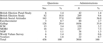
The measure of the policy preferences that we develop in this article is based on all the domestic policy preference data that were available in the Gallup Political Index, British Election Studies (BES), National Opinion Poll (NOP), International Communications and Marketing (ICM), British Social Attitudes (BSA), British Household Panel Study (BHPS), the European Social Survey, Eurobarometer and YouGov (see Table 1). Our search was both lengthy and intensive and so the collection is – within the limits of what one can know – exhaustive.
Sources Used in This Research

Note: Based on June 2007 database (excluding foreign policy items)
The market research industry is still relatively new and subject to change as a result of market conditions and technological change. There are few useful questions in the 1930s, 1940s and even 1950s, when we are reliant on the (now sadly defunct) Gallup Political Index.Footnote 26 Accordingly, we discount our estimates before 1950. Even then, however, the data are thin. We have to rely on a single item in 1950 and 1956 and just four in 1953.Footnote 27 As we move closer to the present day, however, we face an embarrassment of data riches. The peak in terms of both number of questions (N = 147) and separate administrations (N = 161) is 1987, but is still healthy in 2005 (N = 87 in terms of both questions and administrations). We have fully-exploited Gallup, the only possible source of data for the 1950s. Nevertheless, the few items that are available in the 1950s relate to issues such as trade unions and nationalization and – as we demonstrate below – these sorts of items tend to load very heavily on our extracted preference series. Preferences have been so well documented since the 1970s, moreover, that new bits of data are unlikely to make much difference.
As a check on the impact of small numbers of items first and foremost, we have estimated standard errors of our annual estimates. We can estimate a biennial rather than annual time series to see if the main patterns are altered when twice as many items contribute to each estimate. That exercise produces no notable changes.
Indexing Preferences
In order to estimate preferences for government activity, responses were simply coded as either ‘left’ or ‘right’ and ‘neutral’. The latter were discarded from the analysis and an index of preferences calculated:

In general, it is a simple task to decide on the directional thrust of the responses. That is, it was easy to code responses as ‘left’ or ‘right’. This is hardly surprising. British politicians have ‘framed’ many issues in terms of ‘left’ and ‘right’ and survey designers have taken note, thus allowing easy coding of responses.Footnote 28 Moreover, even if we made a mistake in coding, the extraction algorithm would still be able to use the information as long as we had been consistent.
The only major coding difficulty relates to Europe, which has been the subject of data collection efforts since British entry was first floated in 1961. This policy domain arguably lies somewhere between a ‘domestic’ and ‘foreign affairs’ issue, though as integration has increased ‘Europe’ has had a greater impact on domestic policy. The issue has also created divisions on both the left and right for the best part of forty years. The bulk of ‘the right’ tended to support membership of the then European Economic Community and the formation of the single market under the European Community in the 1980s.Footnote 29 As the European Union challenged national sovereignty by moving towards monetary union and developing a ‘social dimension’, however, many on the right became sceptical about the European project. After Mrs Thatcher's removal from office in November 1990, much of the Conservative party drifted to a far more sceptical position and some joined explicitly anti-European parties such as the Referendum Party and the United Kingdom Independence Party. ‘The left’, by contrast, were hopelessly divided on Europe until the late 1980s.Footnote 30 The left tended to oppose membership of the ‘capitalist club’, while moderate social democrats tended to enthusiastically support membership.Footnote 31 It was not until the emergence of a ‘social dimension’ in the early 1990s that being pro-Europe became a ‘left’ position.
Given the detailed knowledge of the European issue, it is tempting to impose the assumption that the ‘polarities’ reversed at some specific date. But pinpointing the exact date would be hazardous and require a fine judgement call. Rather than do this, we (tentatively) code pro-European responses as left and anti-European responses as right. We do not, however, include European items in our estimate of preferences for government activity. This allows us to observe, rather than assume, the relationship between left–right and European preferences.
Self-Reported Left–Right Positions
The most obvious way of estimating voters’ left–right positions is to ask voters to locate themselves on a general left–right scale. At the individual level at least, this method is problematic. Responses to such questions do not express clear preferences over outcomes. They may be empirically related to outcomes but – on the face of it at least – refer simply to the labels that people may attach to themselves. While the small group of politically sophisticated voters may use these labels correctly, the great mass of unsophisticated citizens may not know how to use the labels or know what they mean.Footnote 32 Indeed, it is all too likely that many may guess or infer their left–right position from their understandings of where their parties are located.Footnote 33
Still, it could be argued that, at the aggregate level, these things wash out and that ideological self-location should track real preferences. Variations in reported self-location may, therefore, approximate shifts in preferences. In order to produce a somewhat cleaner set of estimates that is less vulnerable to challenge, however, we exclude these measures from the preferences for government activity series, and – just as with European preferences – we use self-reported left–right positions only to validate these estimates.
In the event, neither of these decisions – to omit European preferences and left–right self-locations – have significant empirical consequences. Indeed, they hardly affect our estimates of the political centre at all.
Estimating the moving centre
Our goal is to locate that – hitherto – mythical median British voter and track him or her over time as preferences change to reflect circumstances. Our device for doing so is (1) to observe raw preferences as expressed in aggregate responses to survey probes about preferred policy choices and (2) to solve for their moving central tendency over time. Policy preferences vary across people and over time. Our interest is only the latter. Thus, at the outset, we score policy preferences as a net disposition across the whole of British society, typically as a percentage choosing the left option (or options) in a question that offers both left and right choices.Footnote 34 Then we observe how that percentage varies over time.
The issue then becomes how to extract the central tendency from a very large number of observed preference series. This is of the class of problems to which principal components analysis – or more loosely, factor analysis – is the solution. Principal components analysis itself is not workable for data of this sort because most of the possible cases – the answers to a potential survey question in year t – are missing. To impute values for those missing cases, which considerably outnumber observed cases, would create a dangerous dependency on the assumptions underlying the imputation. In some cases, those assumptions are relatively benign; for example, a missing year might be well imputed as an average of the years before and after. In many cases, the assumptions are heroic. Imputation might be required to create values for a question series, for example, before it was ever posed the first time and after it was posed the last time.
To deal with the actual structure of the public opinion data we have, we adopt the Dyad Ratios algorithm.Footnote 35 We describe the algorithm briefly here for readers who are not familiar with it. We begin with the data.
What we have for data are numerous series of a single survey item posed to comparable national samples at various times. We wish to estimate the centre for N years (here N = 56) from input data series each of length k, where k is always less than N. We wish to avoid the untenable assumptions (1) that any two different questions are or are not comparable, and (2) that anything can be known about a series in a year that it is not posed.
What that leaves as bedrock knowledge is the assertion that ratios of the responses to the same question at different times are useful information about opinion change.Footnote 36 Each of the two possible cases forms a dyad, and hence the name, dyad ratios algorithm. More formally, assuming that each indicator series is scored to represent left opinion – i.e., larger numbers represent an opinion further to the left – we are asserting that for:

Rij represents a reasonable estimate of how left opinion was in years t+i and t+j. This is not to say that R is a ‘best’ or even ‘good’ estimate of the concept. For a ‘best’ estimate will be efficient in the sense that it is based upon all the information at hand and not merely one arbitrary choice. For each series of length k, we have multiple ratio estimates. These tell us plenty about the years for which the series is measured and nothing about the years when it is not.
Note the gain from switching from raw measures (percentage left) to ratios. In the case of raw measures, a missing case has an unknown expected value.Footnote 37 For a ratio, in contrast, the expected value of the ratio of any two cases is 1.0. That will justify combining estimates derived from different subsets of indicators. No matter what question wording is employed, two valid indicators of the same concept will have the same expected values for ratios.
For multiple series, the question becomes how to combine a very large number of possible ratios into a single estimate. If – a very big if – a single year i were available for all series, then it could serve as a universal base that would give meaning to all the ratios. This is the logic of economic indicators in which a base year is given an arbitrary value, often 100, which then propagates meaningful values to all other years. But this condition is not satisfied by our data. There is no one year where every possible survey question about preferences is posed.
That forces us to choose a next best solution, recursive estimation. Since there is no universal base year for calculation, we form recursive estimates of each year from all the available data pertaining to that year. Thus, we cannot know that Year 2, for example, is 100. But we can know that Year 2 is some computable ratio of Year 1, based on all the data which are available for times 1 and 2. Thus, we let Year 1 be arbitrary, say 100, and then calculate an average Year 1/Year 2 ratio from all the data that connect the two cases to form a best estimate of Year 2 in absolute terms. Then this value can be similarly applied to years 3, 4, … k in the same fashion. This is recursive estimation.
We now have in hand multiple – often multiple hundred – estimates of the same quantity, the absolute leftness of preferences in a particular year, Pt. The large number of overlapping estimates derives from the fact that each series provides k−1 separate estimates of each year where it is available and then there are hundreds of series. A natural first intuition about combining these separate estimates, xtk, is to find their central tendency (denoted Pt for preferences at time t):

But we can do better than that. We know that the items in the analysis are not equally valid indicators of the concept, left–right. Therefore, we can estimate those validities – squared correlations with the latent dimension – and use those estimates to weight items in proportion to their indicator validity, hi 2:

where hi 2 in the numerator is the communality estimate (i.e., validity) of item i and h 2 in the denominator is the average communality across all items.
Recursive estimation can be done forward in time, as described above, or equally well backward. In that case, year T is set to 100 and all earlier years are estimated empirically. The two approaches weight earlier and later cases differently, so that the resulting estimates are not the same. That permits reliability estimation (from the correlations of the two). A final estimate averages the two equally valid approaches.
In principal components, there are three common approaches to the thorny issue of estimating the common variances of individual items. One is to assume (falsely in all actual cases) that each is perfectly valid, in which case 1.0 is the communality estimate placed on the major diagonal of the correlation matrix. A second forms the communality estimate from the R 2 of each indicator regressed on all the others. And a third, usually preferred, approach is iterative. Each iteration begins with assumed communalities from which improved ones can be estimated. Then the improved estimates become assumed values for the next iteration. And so on until convergence is achieved when the difference between the assumed and the estimated is arbitrarily small. The dyad ratios algorithm implements the third, iterative, approach.
Since the recourse to ratios causes the original metric to be lost, it is reintroduced to ease interpretation by a standardization of the latent scale in terms of the validity-weighted means and standard deviations of the input items. Since the individual items are scored as per cent left over per cent left plus per cent right, the resulting scale has the same interpretation. Fifty is a neutral point where left and right alternatives are chosen with equal frequency. Values above 50 indicate a net preference for the left and below 50 a net preference for the right.
The outcome data, as in principal components, tell us for each item how much of its variance is shared with the latent estimated dimension, i.e., its validity, and how heavily it loads on each possible dimension. The latter we employ in the manner of all dimensional analyses to learn what the latent dimensions mean.Footnote 38
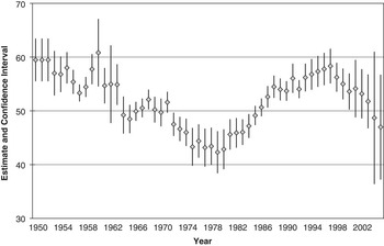
The extracted estimates
Having laid bare the technology, we turn our attention to the estimates. Figure 1 displays our estimate of the public preferences series from 1950 through to 2005. This represents our best estimate of the ‘centre’ in the post-war period. The series starts off high (left) in 1950s and then generally drifts down (right). Pleasingly, this overall pattern seems to agree with several widely praised historical commentaries. In his A History of Modern Britain, for example, Andrew Marr claims that the Second World War ‘changed Britain's political climate and our attitude to government’ and that by 1945 the mood was for ‘big government, digging deep into people's lives to improve them.’Footnote 39 He then (rightly) claims that ‘by the time the last big struggle to nationalise an industry was underway, the steel debates of 1948–49, the public mood was already turning’ and that ‘the government felt a change in the weather’.Footnote 40 Preferences generally continued to drift right until 1979, the very year that Mrs Thatcher came to power.
Estimates of Left–Right Preferences with Confidence Intervals, 1950–2005

Our finding here ties in well with the research of Ivor Crewe and his colleagues, who noted a decline in support for the ‘collectivist trinity’ of public ownership, trade unions and the welfare state from the 1960s through to the 1979 general election.Footnote 41 It also sheds some light on why James Callaghan, then Labour leader and prime minister, confided to his policy adviser during the 1979 general election campaign: ‘You know there are times, perhaps once every thirty years, when there is a sea-change in politics. It then does not matter what you say or what you do. I suspect there is now such a sea change – and it is for Mrs Thatcher.’Footnote 42
Callaghan was clearly correct to say that there had been a ‘sea change’. As our evidence makes clear, however, the change in preferences long pre-dated the specific circumstances of the 1979 general election and the so-called ‘Winter of Discontent’ of 1978/79 that immediately preceded it.
From 1979 onwards, the series tracks remorselessly to the left, peaking in 1997, the year of New Labour's triumph. This finding supports the findings of Crewe, Heath et al. and Crewe and Searing, who find that the electorate generally moved away from ‘Thatcherite’ positions during her period as prime minister.Footnote 43 The series then drifts right again under New Labour, until by 2005 it was roughly where it had been in 1983, the year when Mrs Thatcher won a landslide victory.
The figure shows our best point estimate of left–right policy preferences along with an estimated confidence interval for each annual estimate, which is the point estimate plus or minus two standard errors.Footnote 44 The standard errors reflect how pivotal the various data points are. Variations in particularly important years have relatively large consequences, whereas in most years they do not.
On the face of it, preferences appear to be divided into three distinct periods: moving to the right from the 1950s through to 1979, to the left between 1979 and 1997 and back to the right since 1997. From what we know of British political history, and informed by Wlezien's thermostatic model, it is tempting to link this pattern to variations in the size of the state, which generally expanded in the first period, contracted in the second and then rolled forward again in the third.Footnote 45 It is likely, however, that more directly economic factors also were at play. In the next sections, we examine the validity of the extracted measure by considering which variables are most heavily associated with the estimated series and also its relationship with both left–right self-locations and attitudes towards Europe.
Dimensional analysis
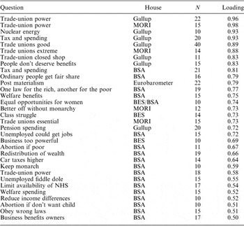
While the picture provided by Figure 1 is generally quite plausible, we need to establish whether the estimates are indeed capturing left–right preferences and movements in the centre. One obvious way of establishing whether our estimated series is indeed capturing preferences for government activity is to examine the loadings for those individual items that make up the scale. Given that the series is based on 349 items asked in 2,482 separate administrations, it would be too messy to display all the loadings. Some items are, moreover, included only twice. While such items would have factor loadings of 1.0 (or −1.0), they would provide a misleading indicator of content. Table 2, therefore, simply reports the highest loadings for only those items that were included in the database on at least ten occasions and load more than 0.50 on the public preferences dimension.Footnote 46
Dimensional Analysis of Preferences Series, 1950–2005

Note: This table contains only those items that are entered into the database in ten separate administrations and have a loading above 0.5.
The first thing to note about Table 2 is that the estimated preference series explains over 43 per cent of the variation in these assorted series. Given the very large number of items, this seems – to us at any rate – quite impressive. More importantly, however, even a brief examination of Table 2 is enough to demonstrate that it is dominated by items relating to trade unions, to the power of business, to taxing and spending and to equality, while the welfare estate, the monarchy and nuclear power also load highly on the scale.
This provides some reassurance that the series is capturing a large part of the battle between Labour and the Conservatives about the extent of state activity. Indeed, we would have been surprised if we had found anything else. It should also be noted, however, that some items that are only remotely related to government activity (such as nuclear power, post-materialism and abortion) also load heavily on the extracted dimension. Put simply, when overall preferences move, so do things that one might think were totally unrelated. This suggests that the extracted dimension is actually picking up something rather more general than preferences for government activity.
Relationship with self-reported left–right positions
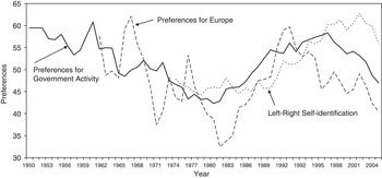
The dimensional analysis contained in Table 2 suggests that the estimate of public preferences reflects a general left–right dimension. But a sceptic might well demand additional confirmation. In this sub-section, we assess the relationship between the series and other measures of left-right position. We are fortunate that the Eurobarometer has asked respondents to report their own left–right positions every year since 1973.Footnote 47 In addition, Gallup and the BES also asked similar questions, somewhat less regularly, in this same period. These series can be combined to generate a single left–right self-placement series using the same extraction algorithm used for the preference series, and we can then examine its relationship with the extracted series (see Figure 2).
Relationship between preferences for government activity, Europe and left–right self locations

Figure 2 also displays the preferences series and self-reported left–right positions from 1973 onwards.Footnote 48 This figure shows that the two series track each other quite well, though reported positions continued to increase (move leftwards) between 1997 and 2002, when policy preferences were decreasing (moving right). This suggests that self-reported positions might be a lagging indicator.Footnote 49 It may simply be that voters who have voted for a ‘left’ party in 1997 and 2001 assume that they must be left too or that social desirability is at play. In any case, the product moment correlation for the two series is an impressive 0.66 (N = 33, p < 0.000). Movements of reported left–right positions are associated with ‘real’ preferences.
It should be finally noted that the correlation between our measure of preferences for government activity without reported left–right positions and the same measure with self-reported positions over the thirty-two years between 1973 and 2005 is a mighty 0.99. It seems that the decision to exclude self-reported left–right positions is more firmly rooted in intuitions about the meaning of ‘preferences’ than in the data. This finding suggests that where preference data are in short supply (in studies of preferences in other countries, for example), changes in self-reported positions might be useful proxies for changes in aggregate preferences.
Relationship with European Preferences
It is unclear whether positions on the European issue are essentially ‘domestic’ or ‘international’ in nature and thus their relationship with ‘left’ and ‘right’ is, furthermore, uncertain. For these reasons, we excluded those items that referred to Europe from the dataset we used to generate our estimates of preferences relating to government activity. Instead, we set these data aside and employed the dyad ratio algorithm to produce a pure measure of latent attitudes towards Europe.
Figure 2 displays preferences relating to Europe from 1961 onwards. The association between the two series in this case does not appear to be quite as good as that for self-reported left–right positions. Nevertheless, the two series generally fit quite well. The 1970s, on the one hand, witnessed a drift to the right in terms of both preferences and a drift towards Euroscepticism. The 1980s, on the other hand, witnessed a drift to the left and increasing support for Europe that reversed itself from around 1991 onwards. The early to mid-1990s combined a slight shift to the left with increased Euroscepticism. From 1997 onwards, the two series marched in step: towards the right and Eurosceptical poles. Yet again, the real test is the correlation between the two series. The product moment correlation for the two is 0.54 (N = 45, p < 0.000). Although it has been suggested that Europe represents a new dimension of British politics, quite separate from the ‘old’ politics of left and right, the data suggest that there is an association between the two.Footnote 50
Figure 2 suggests that our exclusion of reported left–right positions and the European items is more firmly rooted in theoretical considerations than in the data. If we had included the European data in our indicator of preferences, it would have made little difference. The correlation between the two series with and without European items is 0.98. The decision to exclude the European data – like left–right self-reported positions – makes virtually no empirical difference.
Naming the series
We have noted that items relating to taxation, spending and state activity loom large in the preferences series. Since other issues traditionally associated with left and right, such as abortion, nuclear power and post-materialism, also load heavily on the series and since it correlates quite highly with self-reported left–right positions, there seem to be grounds for believing that we have produced a plausible general measure of left–right positions. Indeed, perhaps we should not find this surprising. Theories of ‘issue evolution’ produce the clear expectation that many – even most – issues will eventually be incorporated in the left–right dimension as parties take positions and voters sort themselves into the right parties.Footnote 51 While we are reasonably confident that we have a measure of general left–right positions, we leave it to the reader to decide whether our findings support that proposition.
What moves preferences?
We have shown that preferences move left and right over time. Here, we take on the challenge of explaining why. Most of the movements are small. Indeed, the average annual change, ignoring the sign of the change, is a mere 1.5 points over the full fifty-six years examined here. The largest annual changes occur in 1960–61 (−6.1) and 1964–65 (−5.7), but this may owe a good deal to the thinness of the data at that period (see Figure 1). Beyond this, there is little to suggest that individual events may have affected preferences a great deal. Indeed, such a pattern of small but cumulative change strongly hints at the influence of systemic, macro-level forces.
Theory
To get beneath the longitudinal flow of issue preferences, it is useful to think about the cross-sectional distribution of preferences. Assume that Britain faces a continuing choice of more or fewer government activities and services and the taxes to pay for them.Footnote 52 The extremes of this choice, anarchy at one end and total government at the other, are never attained. Thus, we may think of arraying all citizens into degrees of preferring more or less government and dividing this space of preferences into three groupings, those who want more government than Labour provides, those who want less than the Conservatives provide, and those somewhere in between.Footnote 53
Now, in this hypothetical space, it will be clear that the groups of the extreme left (who want more government than Labour provides) and those of the extreme right (who similarly want less than they ever get from Conservatives) will never be satisfied. Thus, their views should never change. Wanting more (or less) and never getting it implies that they should always continue to want more (or less). That leaves those in between the parties as the only citizens who have a motive to change preferences over time. As control of government alternates between the party of the left and the party of the right, they will see themselves forced to change relative preferences in order to stay constant in absolute terms.Footnote 54
Imagine a citizen in between but relatively close to the Conservatives in preferences. While Conservatives hold power, that citizen will prefer (slightly) more government than he or she gets. When Labour takes control, it will increase the mix of services and taxes and our citizen will soon find that the government is doing more than he or she wished and will need to switch relative preferences to less.
In this story of absolute and relative preferences for the size of government, it is clear that for a rational citizenry the dynamic element is entirely in the middle. Therefore, as we aggregate these preferences and observe them over time, we should observe (1) that all the action is in the centre, and (2) that the dynamics will produce the thermostatic response that Christopher Wlezien hypothesizes.Footnote 55 If we can envision the sum total of public policy on a dimension of more or less government – easy in theory and a little challenging for empirical measurement – then our basic expectation is that citizens will respond to government over time by demanding less of the direction of policy that they are currently receiving.
On to this expectation, which is entirely endogenous to the choices that governments make, we will observe also some factors which are relatively exogenous. Chief among these will be movements in the macro-economy which are capable of altering (absolute) preferences for the level of government. A government experiencing high levels of unemployment, for example, will lead some citizens to prefer a higher level of government activity as a Keynesian response. Thus, independently of our hypothesized timeless basic level of preferred government, some citizens will shift leftwards for a period of time when government is seen as not doing enough to cope with the economic difficulty of unemployment. Inflation provides the reverse case. To the degree that it may be attributed to excess stimulation by government, some citizens might for a period of time rationally prefer less government as a policy response.
From this simple story, we may now formulate empirical expectations of how our observed relative preferences for more or less government will shift over time. Most basically, we expect such preferences to run counter to the dominant flow of policy making, moving left in response to policy of the right and moving right in response to policy of the left. We will take two empirical approaches to this issue. We first expect the direction of preferences to shift in response to party control – which assumes implicitly that parties do what they are supposed to do, Conservatives reducing government and Labour increasing it, which is not always true. Then we will assess our macro-level explanations starting first with economic factors, which predict that unemployment will increase support for government activity and inflation will reduce it. And finally, we will introduce empirical indicators of our size of government concept, average tax levels and government expenditure as a proportion of gross domestic product (GDP).
Analysis
Parties may be ignorant of public opinion, and they may in any case pursue their ideological goals without constant reference to it. In these circumstances, we might expect parties of the left to provide too much government activity and governments of the right too little. In line with Christopher Wlezien's thermostat model, we expect that preferences should move left under the Conservatives and right under Labour.
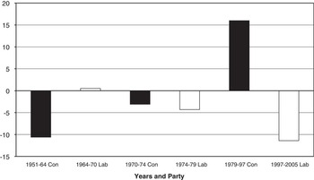
Figure 3 summarizes the changes in preferences under Conservative and Labour governments. This provides some qualified support for the thermostat idea.Footnote 56 The preference series certainly moved right under Labour governments in 1974–79 and in 1997–2005 (see Figure 3). It also moved left under the eighteen years of Conservative rule from 1979 to 1997. Curiously, however, the pattern of changes under the three governments between 1950 and 1974 are in exactly the wrong direction. Preferences move right under the Conservatives in two periods, 1951–64 and 1970–74, and marginally left under Labour in 1964–70. Therefore, we need to take a more systematic look at the phenomenon. For that, we turn to a regression analysis predicting movements of our estimated centre.
Changes in preferences for each government, 1951–2005

We begin our analyses with the simple question of the effect of party control. Although parties can and do vary in the degree to which they pursue distinctive policies, a voter could do reasonably well using the heuristic that Conservatives will tend to reduce the size of government and Labour will tend to increase it. Thus, the simple fact of party control might summarize the idea that preferences move contrary to the dominant direction of policy making.
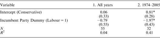
The most basic test of this idea is simply to ask whether the direction of change in preferences responds to the party of government.Footnote 57 We expect the public to move left under Conservative rule and right under Labour. We can tap this with a regression of change of preferences on a party dummy variable (0 = Conservative, 1 = Labour). An initial result is displayed in column 1 of Table 3.
Effects of Party Control of Government on Changes in Preferences

*p < 0.01.
What we see is a result that is correctly signed but not conventionally significant (p < 0.08). The reference category (Conservative) shows changes towards the left (positive sign), albeit very slight, while the Labour category predicts movements towards the right (negative sign). Given what we have seen in Figure 3, this comes as no surprise. During the era of ‘consensus politics’, when Conservative and Labour broadly agreed on the need for a mixed economy and government activity, governments of both parties did things more usually associated with the other party. The governments of the 1950s and early 1960s produced responses sometimes opposite to those predicted by their ideology. The Conservatives expanded state activity in the immediate post-war period and co-operated with the trade unions between 1951 and 1964.Footnote 58 The 1970–74 Heath government initially tried to reduce government activity and then massively expanded it in a famous policy ‘U-turn’.Footnote 59 Equally, the Labour government between 1964 and 1970 had to cut its ambitious spending plans, abandon its ‘national plan’ and tried to introduce legal restraints on the trade unions.Footnote 60
In the second column of Table 3, we restrict analysis to the period beginning in 1974 and pose the same question. For the last thirty-two year period, the expected effect emerges and quite strongly.Footnote 61 The coefficients indicate that every year of Conservative government drives preferences about 0.80 to the left and every year of Labour government pushes preferences even more strongly to the right (−1.97). But our theory is more general. The party dummy variable approach is a crude indicator of the size of government idea. We can do better.
To do so, we need to introduce direct measures of policy making and of economic effects. For economics theory dictates the choice of indicators. We have argued that unemployment shifts net preferences to the left and inflation shifts them to the right. Here, we examine those effects.
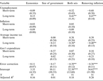
Since we are dealing with a unit root dependent variable (preferences), we employ the error correction framework for analysis. Error correction models assume that the major path of causality between two variables is that the explanatory variables create a dynamic equilibrium for the variable to be explained.Footnote 62 Lacking a fixed mean to which it equilibrates, that is, a unit root variable is thought to equilibrate to a level dependent on the level of the causal series. Thus, when disturbed by some exogenous event or condition, it will tend to equilibrate, but to the dynamic target set by the explanatory variable, not to a fixed mean. The evidence for such dynamic equilibration is in two forms (1) that significant linear relationships are observed between the level of the explanatory series and change in the dependent series (the ‘long-term’ effects of Table 4), and (2) the error correction phenomenon, that changes in the dependent variable are negatively related to its previous deviations from dynamic equilibrium.Footnote 63
Predicting Change in Preferences (Error Correction Models)

*p < 0.05, **p < 0.01, ***p < 0.00.
We begin the analysis of economic effects in Table 4. There, in the column labelled ‘Economics’, we observe the long-term (and short-term) effects of unemployment and inflation on the first differences of preferences. We expect positive long-term effects for unemployment and negative ones for inflation. That is what can be seen in Table 4. But the effects are weak. The error correction is at the margin of significance, the unemployment effect right on the line (p < 0.052), and the inflation long-term effect is correctly signed but not significant. Predicting first differences is a very challenging task, and therefore it is hard to know whether an adjusted R 2 of 0.16 represents success or failure. Overall, we have a hint that economics matters for preferences, but the evidence is far from conclusive.
We do, however, also have two indicators of policy making that might add to our story and permit a more general test of Christopher Wlezien's thermostatic theory. We measure the benefit side of government with government expenditures as a proportion of GDP.Footnote 64 The cost side of government is measured with average income tax.Footnote 65 For both measures, we expect negative long-term effects. Bigger government, that is, should push preferences to the right.
What we observe in Table 4 instead is explanatory failure. The adjusted R 2 of 0.01 tells us what we would also see from the coefficients, that we just have no evidence that (at least taken by itself) the size of government predicts preferences. These outcome variables are perhaps a step too far down the causal chain. They result from the cumulated policies of many governments over a very long span of time and do not necessarily tell us the recent drift of policy making, which may be more influential in driving preferences. With a product moment correlation between them of 0.75, multicollinearity also impedes observing separate effects.
We consider a model which includes both sets of variables in the third column. Here, it becomes clear that both sets are required for a well-specified model. With a better model fit (R 2 = 0.18), the long-term effect of unemployment emerges as a highly significant cause of preference changes as does long-term average taxes. The multicollinear government spending indicator remains correctly signed but non-significant. And inflation, as before, is correctly signed but not powerful enough to attain statistical significance.
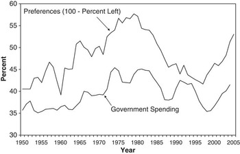
The error correction specification, predicting first differences instead of the level of a series, combined with indicator multicollinearity, can lead to under-appreciation of the true strength of relationships. For another and simpler look at the data, we graph preferences against government spending in Figure 4. This time reversed to indicate right sentiment (i.e., 100 – left), it is quite clear in the graph that government spending and Conservative sentiment move in tandem (r = 0.75). Conservative governments, by cutting government spending, and Labour ones, by increasing it, both seem to sow the seeds of their own demise in policy making. The observed empirical fact of cycles of party control of government may now be seen as the expected outcome of governments pursuing their policy goals instead of heeding the moderating signal of public opinion. It is regularly observed that electorates often express the view that it is time for a change and that there seems to be a political pendulum at work. In this view, however, the pendulum is neither exogenous nor a valence issue but instead the predictable result of macro politics.
The relationship between preferences for government activity and public expenditure
Note: The preference series is reversed (100—left) to measure right sentiment.

For a final test, we remove inflation from the specification and re-estimate the remainder of the terms. This results in strengthening both the unemployment and average tax long-term effects and improving the fit slightly to 0.20. What we now know is that preferences are in a dynamic relationship with unemployment rates and with the size of government (with either indicator separately or average taxes jointly). That means that those two variables set an appropriate target level for preferences. And it tells us that when actual preferences move away from that target, they tend to correct back to it fairly rapidly. The estimated error correction rate (0.38) tells us that almost 40 per cent of any deviation of preferences from the target rate in either direction is corrected within one year.Footnote 66 Public preferences do respond to the size of government and to the state of the national economy. Ivor Crewe's observation that British elections are a matter of ‘the economy and public services, stupid’ seems to apply equally to preferences.Footnote 67 And since the British state provides things that are in the United States provided by the market, this apparent difference from the United States makes some sense.
So what? a first look at preferences and elections
A natural reaction to the results in the previous section is, so what? While we believe that preferences are important things to study in themselves, most readers are interested in them only in so far as they influence election outcomes.Footnote 68 In this penultimate section, we examine briefly the relationship between preferences and elections. Before we do so, however, it is worth noting that there are some reasons not to expect a direct relationship between opinion and elections. Politicians are generally smart operators with a real incentive to learn about voters. If opinion is shifting, they are likely to respond and close the distance if at all possible (though they may face tight ideological constraints). As modellers, moreover, we face a series of obstacles. If spatial theories of elections are to be believed, electoral outcomes are driven by the distance between parties and the average or median voter. To construct a model of election outcomes, therefore, we need both a valid measure of party positions and some way of mapping voters and parties onto the same scale. This is a large task and one that we must necessarily postpone to another paper.Footnote 69
Nevertheless, the preference series displayed in Figure 2 provides an interesting perspective on election outcomes. As David Butler has suggested, elections ‘have registered the change of mood that events and political rhetoric have wrought, month by month, in the voters’ minds.’Footnote 70 It is clear, however, that changes in preferences often long pre-date election outcomes. Both Mrs Thatcher's victory in 1979 and New Labour's triumph in 1997 are fully anticipated in the series. Nevertheless, it seems that preferences in 1979 (the year of Mrs Thatcher's first election) were not very different, for example, from those in 1974 (the year of Labour's two narrow victories).Footnote 71 James Callaghan's fatalism in spring 1979 may have reflected not only his (then recent) experiences during the Winter of Discontent, but the cumulative realization that public support for government activity had been eroded over the preceding thirty years.
Equally, preferences in 1997 (the year of New Labour's victory) do not look so very different from those five years earlier (when the Conservative party won a fourth consecutive victory). This latter finding may help explain why the electorate turned against the Conservatives so quickly – and so decisively – after the ‘Black Wednesday’ crisis in September 1992. Kenneth Newton suggested that the 1992 election campaign was in many ways a contest between ‘caring’ (Labour) and ‘competence’ (Conservative).Footnote 72 It may simply be that many had voted Conservative in April 1992 despite their ideological dispositions. Many voters did ‘care’ about unemployment and the state of the public services but concluded that the Conservatives would be more ‘competent’ when it came to managing the economy than their Labour rivals. If this is true, then many voted Conservative with a heavy heart and may have felt like fools when Britain was forced to leave the ERM in September 1992. What may have hitherto been missing from accounts of ‘Black Wednesday’ is the observation that the electorate's ‘hearts’ were with Labour in 1992, though many were undoubtedly eventually ruled by their ‘heads’ and voted Conservative. Equally, while David Sanders is clearly correct in arguing that New Labour's victory in 1997 owed much to its move to the centre between 1992 and 1997, it also owed a great deal to the shift in preferences that had happened by 1992.Footnote 73
To bring the story up to date, it appears that some of Labour's losses in 2001 and 2005 may well be due to shifts in preferences. We know that preferences fell from around 58 in 1997 to approximately 49 points in 2005 (presumably as a result of the massive increases in spending and taxation following on from Gordon Brown's comprehensive spending review in August 2000).Footnote 74 The Comparative Manifesto Project (CMP) analyses suggest that Labour moved left slightly between 1997 and 2001 and again between 2001 and 2005.Footnote 75 These shifts in party position were not large, but – when coupled with the drift to the right in preferences documented in Figure 2 – it seems plausible to suggest that Labour's losses may owe something to the increasing ‘distance’ between themselves and the electorate.Footnote 76 To be sure, they may also be the result of a diminished valence advantage and the negative effects of the Iraq War. The evidence from our preference series, however, certainly hints at an additional proximity factor. And the reasons for this increased distance were movement by both the party and the electorate.
In due course, we hope to produce a single model of election outcomes for the period between 1950 and 2005. This will represent the closest thing approximating to a general model of elections that has yet been produced in Britain. It may then be possible to run simulations that will help resolve nagging questions, such as whether New Labour's shift to ‘the centre’ was necessary for it to win in 1997. As we have noted, however, that will require the imposition of some additional assumptions and is, therefore, a matter for further research.
Conclusions
In recent years, political scientists are rightly concerned with replication and the need to demonstrate that empirical generalizations hold across time and space.Footnote 77 It is heartening, therefore, that this article has provided corroboration of studies of the US macro polity.Footnote 78 It has, for example, demonstrated that it is possible to track shifts in the political centre in Britain between using hard evidence drawn from survey data rather than – as was so often the case in the past – informed speculation. It has also demonstrated that – just as in the United States – the centre appears to move over long periods of time and that it moves in response to government activity. And it has gone beyond these US studies by examining the role of taxation and spending. When unemployment has risen or the share of the national wealth devoted to public spending has declined, the electorate has, on average, moved left. When taxes and spending have increased, the electorate has, on average shifted right. This provides support for Christopher Wlezien's thermostatic conception of public opinion generalized across the whole of government activity.Footnote 79 It also provides an explanation of the ‘costs of ruling’: the tendency of governments to lose support whatever the state of the economy.Footnote 80 This may be partly the result of governing parties following their ideological convictions about the scope of government activity. It will certainly be interesting to see whether these findings hold in other European countries and whether government spending has the same effect in the United States.
Our findings suggest that students of political behaviour should pay greater attention to those large-scale movements of opinion that occur over the long haul. It is all too easy to dismiss minor changes in survey marginal responses, but when these take place across a wide range of specific issues, they may tell us that something important is under way.Footnote 81 Movements in public preferences may provide clues about both the likely direction of policy and electoral outcomes (though this is a matter for future research). These sorts of macro-level analyses provide an interesting and – to our minds – compelling alternative perspective to the more familiar micro-level studies. And, quite unlike such individual-level studies, they permit us to examine the origins of those preferences and their relation to real or objectively measured causes, such as the economy.
Taken as a whole, these findings also provide support for the proposition that one can agree that the average citizen is not particularly informed, not particularly thoughtful, and not particularly attentive, but still find these characteristics emerge in the aggregate.Footnote 82 The apparent responsiveness of preferences to government activity does something to salvage the reputation of the electorate. Our analyses provide clear evidence for the proposition that the electorate – when taken as an aggregate whole – is responsive to real outcomes.Footnote 83
The political centre is a concept of enormous analytical importance and the estimates provided here can be used in a wide range of research. In our own research, we intend to provide more analyses of the dimensions underlying the preferences.Footnote 84 We will assess the impact of party proximity to the political centre on aggregate vote share (and possibly approval of the government's record). Ultimately, of course, we also wish to assess the quality of representation by determining the relationship between preferences and government activity. Only then will we be able to assess whether there is indeed a necessary relationship between what the public wants and what they actually get.