2 Governing equations and numerical method

The following dimensionless Navier–Stokes equations in conservative form are solved numerically in this study (Wang et al. Reference Wang, Wang, Xiao, Shi and Chen2010, Reference Wang, Wan, Chen and Chen2018a )

(2.1) $$\begin{eqnarray}\displaystyle & \displaystyle \frac{\unicode[STIX]{x2202}\unicode[STIX]{x1D70C}}{\unicode[STIX]{x2202}t}+\frac{\unicode[STIX]{x2202}(\unicode[STIX]{x1D70C}u_{j})}{\unicode[STIX]{x2202}x_{j}}=0, & \displaystyle\end{eqnarray}$$

(2.2) $$\begin{eqnarray}\displaystyle & \displaystyle \frac{\unicode[STIX]{x2202}(\unicode[STIX]{x1D70C}u_{i})}{\unicode[STIX]{x2202}t}+\frac{\unicode[STIX]{x2202}[\unicode[STIX]{x1D70C}u_{i}u_{j}+p\unicode[STIX]{x1D6FF}_{ij}]}{\unicode[STIX]{x2202}x_{j}}=\frac{1}{Re}\frac{\unicode[STIX]{x2202}\unicode[STIX]{x1D70E}_{ij}}{\unicode[STIX]{x2202}x_{j}}+{\mathcal{F}}_{i}, & \displaystyle\end{eqnarray}$$

(2.3) $$\begin{eqnarray}\displaystyle & \displaystyle \frac{\unicode[STIX]{x2202}{\mathcal{E}}}{\unicode[STIX]{x2202}t}+\frac{\unicode[STIX]{x2202}[({\mathcal{E}}+p)u_{j}]}{\unicode[STIX]{x2202}x_{j}}=\frac{1}{\unicode[STIX]{x1D6FC}}\frac{\unicode[STIX]{x2202}}{\unicode[STIX]{x2202}x_{j}}\left(\unicode[STIX]{x1D705}\frac{\unicode[STIX]{x2202}T}{\unicode[STIX]{x2202}x_{j}}\right)+\frac{1}{Re}\frac{\unicode[STIX]{x2202}(\unicode[STIX]{x1D70E}_{ij}u_{i})}{\unicode[STIX]{x2202}x_{j}}-\unicode[STIX]{x1D6EC}+{\mathcal{F}}_{I}+{\mathcal{F}}_{j}u_{j}, & \displaystyle\end{eqnarray}$$

(2.4) $$\begin{eqnarray}\displaystyle & p=\unicode[STIX]{x1D70C}T/(\unicode[STIX]{x1D6FE}M^{2}), & \displaystyle\end{eqnarray}$$

where $\unicode[STIX]{x1D70C}$ is the density, $u_{i}$ is the velocity component, $p$ is the pressure and $T$ is the temperature. The viscous stress $\unicode[STIX]{x1D70E}_{ij}$ is defined by

(2.5) $$\begin{eqnarray}\unicode[STIX]{x1D70E}_{ij}=\unicode[STIX]{x1D707}\left(\frac{\unicode[STIX]{x2202}u_{i}}{\unicode[STIX]{x2202}x_{j}}+\frac{\unicode[STIX]{x2202}u_{j}}{\unicode[STIX]{x2202}x_{i}}\right)-\frac{2}{3}\unicode[STIX]{x1D707}\unicode[STIX]{x1D703}\unicode[STIX]{x1D6FF}_{ij},\end{eqnarray}$$

where, $\unicode[STIX]{x1D703}=\unicode[STIX]{x2202}u_{k}/\unicode[STIX]{x2202}x_{k}$ is the normalized velocity divergence; ${\mathcal{F}}_{i}$ is a large-scale forcing to the fluid momentum, ${\mathcal{F}}_{I}$ is a large-scale forcing to the internal energy and $\unicode[STIX]{x1D6EC}$ is a large-scale cooling function per unit volume. The total energy per unit volume ${\mathcal{E}}$ is defined by

(2.6) $$\begin{eqnarray}{\mathcal{E}}=\frac{p}{\unicode[STIX]{x1D6FE}-1}+\frac{1}{2}\unicode[STIX]{x1D70C}(u_{j}u_{j}).\end{eqnarray}$$

A set of reference scales can be introduced to normalize the hydrodynamic and thermodynamic variables in compressible turbulence, including the reference length  $L_{f}$ , velocity  $U_{f}$ , density  $\unicode[STIX]{x1D70C}_{f}$ , pressure $p_{f}=\unicode[STIX]{x1D70C}_{f}U_{f}^{2}$ , temperature  $T_{f}$ , energy per unit volume $\unicode[STIX]{x1D70C}_{f}U_{f}^{2}$ , viscosity  $\unicode[STIX]{x1D707}_{f}$ and thermal conductivity $\unicode[STIX]{x1D705}_{f}$ respectively. After normalization, three reference governing parameters are obtained: the reference Reynolds number $Re\equiv \unicode[STIX]{x1D70C}_{f}U_{f}L_{f}/\unicode[STIX]{x1D707}_{f}$ , the reference Mach number $M=U_{f}/c_{f}$ and the reference Prandtl number $Pr\equiv \unicode[STIX]{x1D707}_{f}C_{p}/\unicode[STIX]{x1D705}_{f}$ . Here, the speed of sound is defined by $c_{f}\equiv \sqrt{\unicode[STIX]{x1D6FE}RT_{f}}$ ; $\unicode[STIX]{x1D6FE}\equiv C_{p}/C_{v}$ is the ratio of specific heat at constant pressure $C_{p}$ to that at constant volume $C_{v}$ , which is assumed to be equal to 1.4, $R$ is the specific gas constant. The parameter $\unicode[STIX]{x1D6FC}$ is defined by $\unicode[STIX]{x1D6FC}\equiv Pr\,Re(\unicode[STIX]{x1D6FE}-1)M^{2}$ . It is assumed that the parameter $Pr$ is equal to 0.7.

We apply Sutherland’s law for the non-dimensional temperature-dependent viscosity coefficient $\unicode[STIX]{x1D707}$ and thermal conductivity coefficient $\unicode[STIX]{x1D705}$ (Wang et al. Reference Wang, Wang, Xiao, Shi and Chen2010). We apply large-scale forcing to the solenoidal velocity component and internal energy by fixing the spectrum within the two lowest wavenumber shells (Chen & Cao Reference Chen and Cao1997; Wang et al. Reference Wang, Wang, Xiao, Shi and Chen2010; Donzis & Maqui Reference Donzis and Maqui2016). We also employ a uniform thermal cooling $\unicode[STIX]{x1D6EC}$ to sustain the internal energy in a statistically steady state (Wang et al. Reference Wang, Wang, Xiao, Shi and Chen2010).

We utilize a hybrid numerical method (Wang et al. Reference Wang, Wang, Xiao, Shi and Chen2010) to simulate stationary three-dimensional compressible isotropic turbulence with a heat source in a cubic box at a $1024^{3}$ grid resolution. The hybrid scheme combines an eighth-order compact finite difference scheme (Lele Reference Lele1992) for smooth regions and a seventh-order weighted essentially non-oscillatory (WENO) scheme (Balsara & Shu Reference Balsara and Shu2000) for shock regions. Some grid refinement studies of the hybrid scheme for a turbulent Mach number around 1.0 were performed in previous works (Wang et al. Reference Wang, Shi, Wang, Xiao, He and Chen2011, Reference Wang, Shi, Wang, Xiao, He and Chen2012).

The dynamical equation of temperature $T$ can be derived as (Sagaut & Cambon Reference Sagaut and Cambon2008; Wang et al. Reference Wang, Gotoh and Watanabe2017):

(2.7) $$\begin{eqnarray}\frac{\unicode[STIX]{x2202}T}{\unicode[STIX]{x2202}t}+u_{j}\frac{\unicode[STIX]{x2202}T}{\unicode[STIX]{x2202}x_{j}}=-(\unicode[STIX]{x1D6FE}-1)T\unicode[STIX]{x1D703}+D_{\unicode[STIX]{x1D705}}+D_{\unicode[STIX]{x1D707}}+f_{T},\end{eqnarray}$$

where the thermal diffusion term $D_{\unicode[STIX]{x1D705}}$ and the viscous dissipation term $D_{\unicode[STIX]{x1D707}}$ are given by $D_{\unicode[STIX]{x1D705}}=(1/\unicode[STIX]{x1D70C}c_{v})(\unicode[STIX]{x2202}/\unicode[STIX]{x2202}x_{j})(\unicode[STIX]{x1D705}(\unicode[STIX]{x2202}T/\unicode[STIX]{x2202}x_{j}))$ and $D_{\unicode[STIX]{x1D707}}=(1/Re)(\unicode[STIX]{x1D70E}_{ij}/\unicode[STIX]{x1D70C}c_{v})(\unicode[STIX]{x2202}u_{i}/\unicode[STIX]{x2202}x_{j})$ , respectively. Here $c_{v}=1/(\unicode[STIX]{x1D6FE}(\unicode[STIX]{x1D6FE}-1)M^{2})$ . The effect of large-scale forcing is represented by  $f_{T}$ .

Temperature can be decomposed into a spatially averaged value $T_{0}$ and a fluctuating value  $T_{1}$ : $T=T_{0}+T_{1}$ , where $T_{0}=\langle T\rangle$ . The equation for the root-mean-square (r.m.s.) value of temperature can be written as:

(2.8) $$\begin{eqnarray}\frac{\unicode[STIX]{x2202}}{\unicode[STIX]{x2202}t}\langle T_{1}^{2}\rangle =\unicode[STIX]{x1D716}_{T}^{inj}-\unicode[STIX]{x1D716}_{T},\end{eqnarray}$$

where, the total dissipation rate of temperature is $\unicode[STIX]{x1D716}_{T}=\unicode[STIX]{x1D716}_{T}^{\unicode[STIX]{x1D703}}+\unicode[STIX]{x1D716}_{T}^{\unicode[STIX]{x1D705}}+\unicode[STIX]{x1D716}_{T}^{\unicode[STIX]{x1D707}}$ . The dissipation rates due to dilatation, thermal diffusion and viscous dissipation are, respectively, $\unicode[STIX]{x1D716}_{T}^{\unicode[STIX]{x1D703}}=-(3-2\unicode[STIX]{x1D6FE})\langle T_{1}^{2}\unicode[STIX]{x1D703}\rangle +2(\unicode[STIX]{x1D6FE}-1)T_{0}\langle T_{1}\unicode[STIX]{x1D703}\rangle$ , $\unicode[STIX]{x1D716}_{T}^{\unicode[STIX]{x1D705}}=2\langle \unicode[STIX]{x1D705}(\unicode[STIX]{x2202}T_{1}/\unicode[STIX]{x2202}x_{j})(\unicode[STIX]{x2202}/\unicode[STIX]{x2202}x_{j})(T_{1}/\unicode[STIX]{x1D70C}c_{v})\rangle$ and $\unicode[STIX]{x1D716}_{T}^{\unicode[STIX]{x1D707}}=-2\langle (1/Re)(T_{1}\unicode[STIX]{x1D70E}_{ij}/\unicode[STIX]{x1D70C}c_{v})(\unicode[STIX]{x2202}u_{i}/\unicode[STIX]{x2202}x_{j})\rangle$ ; $\unicode[STIX]{x1D716}_{T}^{inj}=2\langle T_{1}f_{T}\rangle$ represents the injection of temperature fluctuations by large-scale forcing.

The dynamical equation for the dimensionless entropy per unit mass $s=\log (T/\unicode[STIX]{x1D70C}^{\unicode[STIX]{x1D6FE}-1})$ can be readily derived as (Bayly et al. Reference Bayly, Levermore and Passot1992; Eyink & Drivas Reference Eyink and Drivas2018):

(2.9) $$\begin{eqnarray}\frac{\unicode[STIX]{x2202}s}{\unicode[STIX]{x2202}t}+u_{j}\frac{\unicode[STIX]{x2202}s}{\unicode[STIX]{x2202}x_{j}}=\frac{1}{T}D_{\unicode[STIX]{x1D705}}+\frac{1}{T}D_{\unicode[STIX]{x1D707}}+\frac{1}{T}\,f_{T}.\end{eqnarray}$$

Equation (2.9) is similar to the passive scalar transport equation. The equation for the r.m.s. value of entropy can be written as:

(2.10) $$\begin{eqnarray}\frac{\unicode[STIX]{x2202}}{\unicode[STIX]{x2202}t}\langle (s_{1})^{2}\rangle =\unicode[STIX]{x1D716}_{s}^{inj}-\unicode[STIX]{x1D716}_{s},\end{eqnarray}$$

where, $s_{1}=s-s_{0}$ , $s_{0}=\langle s\rangle$ and the total dissipation rate of entropy is $\unicode[STIX]{x1D716}_{s}=\unicode[STIX]{x1D716}_{s}^{\unicode[STIX]{x1D703}}+\unicode[STIX]{x1D716}_{s}^{\unicode[STIX]{x1D705}}+\unicode[STIX]{x1D716}_{s}^{\unicode[STIX]{x1D707}}$ . The dissipation rates due to dilatation, thermal diffusion and viscous dissipation are, respectively, $\unicode[STIX]{x1D716}_{s}^{\unicode[STIX]{x1D703}}=-\langle s_{1}^{2}\unicode[STIX]{x1D703}\rangle$ , $\unicode[STIX]{x1D716}_{s}^{\unicode[STIX]{x1D705}}=2\langle \unicode[STIX]{x1D705}(\unicode[STIX]{x2202}T/\unicode[STIX]{x2202}x_{j})(\unicode[STIX]{x2202}/\unicode[STIX]{x2202}x_{j})(s_{1}/c_{v}\unicode[STIX]{x1D70C}T)\rangle$ and $\unicode[STIX]{x1D716}_{s}^{\unicode[STIX]{x1D707}}=-2\langle (1/Re)(s_{1}\unicode[STIX]{x1D70E}_{ij}/c_{v}\unicode[STIX]{x1D70C}T)(\unicode[STIX]{x2202}u_{i}/\unicode[STIX]{x2202}x_{j})\rangle$ ; $\unicode[STIX]{x1D716}_{s}^{inj}=2\langle s_{1}f_{T}/T\rangle$ represents the injection of entropy fluctuations by large-scale forcing.

3 One-point statistics of compressible turbulence

Overall statistics for simulated compressible turbulent flows are given in table 1. The Taylor microscale Reynolds number $Re_{\unicode[STIX]{x1D706}}$ and the turbulent Mach number $M_{t}$ are defined, respectively by (Wang et al. Reference Wang, Wan, Chen and Chen2018a )

(3.1a,b ) $$\begin{eqnarray}Re_{\unicode[STIX]{x1D706}}=Re\frac{\langle \unicode[STIX]{x1D70C}\rangle u^{\prime }\unicode[STIX]{x1D706}}{\sqrt{3}\langle \unicode[STIX]{x1D707}\rangle },\quad M_{t}=M\frac{u^{\prime }}{\langle \sqrt{T}\rangle },\end{eqnarray}$$

where $\langle \,\rangle$ stands for spatial average. The r.m.s. velocity magnitude is $u^{\prime }=\sqrt{\langle u_{1}^{2}+u_{2}^{2}+u_{3}^{2}\rangle }$ and the Taylor microscale is

(3.2) $$\begin{eqnarray}\unicode[STIX]{x1D706}=\sqrt{\frac{\langle u_{1}^{2}+u_{2}^{2}+u_{3}^{2}\rangle }{\langle (\unicode[STIX]{x2202}u_{1}/\unicode[STIX]{x2202}x_{1})^{2}+(\unicode[STIX]{x2202}u_{2}/\unicode[STIX]{x2202}x_{2})^{2}+(\unicode[STIX]{x2202}u_{3}/\unicode[STIX]{x2202}x_{3})^{2}\rangle }}.\end{eqnarray}$$

The Taylor Reynolds numbers $Re_{\unicode[STIX]{x1D706}}$ are close to 250 in the numerical simulations. Two turbulent Mach numbers are considered: $M_{t}=0.2$ and $M_{t}=0.6$ .

Table 1.

Simulation parameters and resulting flow statistics.

The Kolmogorov length scale $\unicode[STIX]{x1D702}$ of compressible turbulence is defined by (Wang et al. Reference Wang, Wan, Chen and Chen2018a )

(3.3) $$\begin{eqnarray}\unicode[STIX]{x1D702}=[\langle \unicode[STIX]{x1D707}/(Re\,\unicode[STIX]{x1D70C})\rangle ^{3}/\unicode[STIX]{x1D716}]^{1/4},\end{eqnarray}$$

where $\unicode[STIX]{x1D716}$ is the spatial average of the viscous dissipation rate of kinetic energy per unit mass:

(3.4) $$\begin{eqnarray}\unicode[STIX]{x1D716}=\frac{1}{\langle \unicode[STIX]{x1D70C}\rangle }\left\langle \frac{\unicode[STIX]{x1D70E}_{ij}S_{ij}}{Re}\right\rangle .\end{eqnarray}$$

The resolution parameter $\unicode[STIX]{x1D702}/\unicode[STIX]{x0394}x$ is in the range $1.07\leqslant \unicode[STIX]{x1D702}/\unicode[STIX]{x0394}x\leqslant 1.09$ in the numerical simulations, where $\unicode[STIX]{x0394}x$ denotes the grid length in each direction. Consequently, the resolution parameter $k_{max}\unicode[STIX]{x1D702}$ is in the range $3.36\leqslant k_{max}\unicode[STIX]{x1D702}\leqslant 3.42$ , where the largest wavenumber $k_{max}$ is half of the number of grids $N$ in each direction: $k_{max}=N/2=\unicode[STIX]{x1D70B}/\unicode[STIX]{x0394}x$ . Previous grid refinement studies showed that grid resolutions $k_{max}\unicode[STIX]{x1D702}\geqslant 3.3$ are enough for the convergence of flow statistics, including the kinetic energy spectrum at different wavenumbers and the probability density functions (PDFs) of velocity divergence and vorticity (Wang et al. Reference Wang, Shi, Wang, Xiao, He and Chen2011, Reference Wang, Shi, Wang, Xiao, He and Chen2012).

By applying the Helmholtz decomposition, we decompose the velocity field $\boldsymbol{u}$ into a solenoidal component $\boldsymbol{u}^{S}$ and a compressible component $\boldsymbol{u}^{C}$ (Samtaney, Pullin & Kosovic Reference Samtaney, Pullin and Kosovic2001; Sagaut & Cambon Reference Sagaut and Cambon2008; Wang et al. Reference Wang, Shi, Wang, Xiao, He and Chen2012):

(3.5) $$\begin{eqnarray}\boldsymbol{u}=\boldsymbol{u}^{S}+\boldsymbol{u}^{C},\end{eqnarray}$$

where $\unicode[STIX]{x1D735}\boldsymbol{\cdot }\boldsymbol{u}^{S}=0$ and $\unicode[STIX]{x1D735}\times \boldsymbol{u}^{C}=0$ . The r.m.s. values of the solenoidal and compressible velocity components are defined by $u_{rms}^{S}=\sqrt{\langle (u_{1}^{S})^{2}+(u_{2}^{S})^{2}+(u_{3}^{S})^{2}\rangle }$ and $u_{rms}^{C}=\sqrt{\langle (u_{1}^{C})^{2}+(u_{2}^{C})^{2}+(u_{3}^{C})^{2}\rangle }$ , respectively. It is shown that $u_{rms}^{S}$ is close to $u^{\prime }$ , while $u_{rms}^{C}$ is significantly smaller than $u_{rms}^{S}$ , implying that the solenoidal velocity component is predominant over its compressible counterpart.

The total dissipation rate of kinetic energy per unit mass is given by

(3.6) $$\begin{eqnarray}\unicode[STIX]{x1D716}_{K}=\frac{1}{\langle \unicode[STIX]{x1D70C}\rangle }\left[-\langle p\unicode[STIX]{x1D703}\rangle +\left\langle \frac{\unicode[STIX]{x1D70E}_{ij}S_{ij}}{Re}\right\rangle \right],\end{eqnarray}$$

namely, the total conversion rate of kinetic energy into internal energy by the pressure dilatation $-\langle p\unicode[STIX]{x1D703}\rangle /\langle \unicode[STIX]{x1D70C}\rangle$ and the viscous dissipation  $\unicode[STIX]{x1D716}$ . It is found that the magnitude of $-\langle p\unicode[STIX]{x1D703}\rangle /\langle \unicode[STIX]{x1D70C}\rangle$ is much smaller than that of  $\unicode[STIX]{x1D716}$ , and the value of $\unicode[STIX]{x1D716}$ is very close to that of  $\unicode[STIX]{x1D716}_{K}$ .

Table 2.

Statistics of thermodynamic variables.

The dimensionless entropy is given by $s=\log (T/\unicode[STIX]{x1D70C}^{\unicode[STIX]{x1D6FE}-1})$ . The average values of pressure, density, temperature and entropy are given by $p_{0}=\langle p\rangle$ , $\unicode[STIX]{x1D70C}_{0}=\langle \unicode[STIX]{x1D70C}\rangle$ , $T_{0}=\langle T\rangle$ , $s_{0}=\langle s\rangle$ . The average density is $\unicode[STIX]{x1D70C}_{0}=1$ in the numerical simulations. The r.m.s. values of pressure, density, temperature and entropy are defined by: $p_{rms}=\sqrt{\langle (p-p_{0})^{2}\rangle }$ , $\unicode[STIX]{x1D70C}_{rms}=\sqrt{\langle (\unicode[STIX]{x1D70C}-\unicode[STIX]{x1D70C}_{0})^{2}\rangle }$ , $T_{rms}=\sqrt{\langle (T-T_{0})^{2}\rangle }$ and $s_{rms}=\sqrt{\langle (s-s_{0})^{2}\rangle }$ , respectively. The one-point statistics of thermodynamic variables are given in table 2. We observe that $p_{rms}/p_{0}$ increases rapidly with the turbulent Mach number, while $\unicode[STIX]{x1D70C}_{rms}/\unicode[STIX]{x1D70C}_{0}$ , $T_{rms}/T_{0}$ and $s_{rms}$ are insensitive to the change of turbulent Mach number. Previous studies showed that if the compressible velocity component is dominated by acoustic waves, there are equipartition relations between pressure and the compressible velocity component in weak and strong forms (Sarkar et al. Reference Sarkar, Erlebacher, Hussaini and Kreiss1991; Sagaut & Cambon Reference Sagaut and Cambon2008; Jagannathan & Donzis Reference Jagannathan and Donzis2016; Wang et al. Reference Wang, Gotoh and Watanabe2017; Chen et al. Reference Chen, Wang, Li, Wan and Chen2018; Wang et al. Reference Wang, Wan, Chen, Xie and Chen2018b ). The weak acoustic equilibrium can be expressed as

(3.7) $$\begin{eqnarray}p_{rms}\approx \unicode[STIX]{x1D70C}_{0}c_{0}u_{rms}^{C},\end{eqnarray}$$

where, $c_{0}=\sqrt{\unicode[STIX]{x1D6FE}p_{0}/\unicode[STIX]{x1D70C}_{0}}$ is the speed of sound. The above relation is equivalent to

(3.8) $$\begin{eqnarray}\frac{\sqrt{\unicode[STIX]{x1D6FE}\unicode[STIX]{x1D70C}_{0}p_{0}}u_{rms}^{C}}{p_{rms}}\approx 1.\end{eqnarray}$$

As shown in table 2, $\sqrt{\unicode[STIX]{x1D6FE}\unicode[STIX]{x1D70C}_{0}p_{0}}u_{rms}^{C}/p_{rms}$ is close to 1 in the numerical simulations, implying that the compressible velocity component is dominated by acoustic waves.

4 Spectra of velocity and thermodynamic variables

The compensated spectrum $E^{u}(k)\unicode[STIX]{x1D716}^{-2/3}k^{5/3}$ of the velocity field is plotted in figure 1(a). The velocity spectrum $E^{u}(k)$ satisfies $\int _{0}^{\infty }E^{u}(k)\,\text{d}k=\langle \boldsymbol{u}^{2}\rangle /2$ . An inertial range of the velocity spectrum is observed, namely, $E^{u}(k)k^{5/3}\unicode[STIX]{x1D716}^{-2/3}k^{5/3}\approx C_{K}$ , where the Kolmogorov constant $C_{K}$ is approximately 1.6, which is similar to the previous results of the velocity spectrum in compressible isotropic turbulence (Wang et al. Reference Wang, Shi, Wang, Xiao, He and Chen2012; Jagannathan & Donzis Reference Jagannathan and Donzis2016; Wang et al. Reference Wang, Gotoh and Watanabe2017). The compensated spectrum $E^{u,C}(k)\unicode[STIX]{x1D716}^{-2/3}k^{5/3}$ of the compressible velocity component is depicted in figure 1(b). The spectrum of compressible velocity $E^{u,C}(k)$ satisfies $\int _{0}^{\infty }E^{u,C}(k)\,\text{d}k=\langle (u^{C})^{2}/2\rangle$ . It is found that $E^{u,C}(k)k^{5/3}\unicode[STIX]{x1D716}^{-2/3}\approx 0.2$ and 0.1 respectively for $M_{t}=0.2$ and 0.6 for a short range of wavenumbers $0.015\leqslant k\unicode[STIX]{x1D702}\leqslant 0.05$ . The $k^{-5/3}$ scaling of compressible velocity spectrum $E^{u,C}(k)$ was also observed at $M_{t}\geqslant 0.6$ in solenoidally forced stationary compressible isotropic turbulence without any heat source, where the acoustic mode dominates the dynamics of the compressible velocity component (Wang et al. Reference Wang, Gotoh and Watanabe2017). In the previous study, the $k^{-3}$ scaling of the compressible velocity spectrum was identified in the range of wavenumber where the pseudosound mode is predominant over the acoustic mode at $M_{t}=0.2$ (Wang et al. Reference Wang, Gotoh and Watanabe2017). In contrast, we observe the $k^{-5/3}$ scaling of the compressible velocity spectrum at $M_{t}=0.2$ in this study. The different scaling behaviour of the compressible velocity spectrum can be attributed to the fact that the heat source can generate acoustic waves which dominate the dynamics of the compressible velocity component at $M_{t}=0.2$ .

Figure 1.

Compensated spectra of velocity and compressible velocity component at $M_{t}=0.2$ , 0.6: (a)  $E^{u}(k)k^{5/3}\unicode[STIX]{x1D716}^{-2/3}$ ; (b)  $E^{u,C}(k)k^{5/3}\unicode[STIX]{x1D716}^{-2/3}$ .

Figure 2.

Normalized spectra of density and pressure at $M_{t}=0.2$ , 0.6: (a)  $E^{\unicode[STIX]{x1D70C}}(k)/(\unicode[STIX]{x1D70C}_{rms})^{2}$ ; (b)  $E^{p}(k)/(p_{rms})^{2}$ .

The normalized density fluctuation spectrum $E^{\unicode[STIX]{x1D70C}}(k)/(\unicode[STIX]{x1D70C}_{rms})^{2}$ and normalized pressure fluctuation spectrum $E^{p}(k)/(p_{rms})^{2}$ are plotted in figure 2, where $E^{\unicode[STIX]{x1D70C}}(k)$ and $E^{p}(k)$ satisfy $\int _{0}^{\infty }E^{\unicode[STIX]{x1D70C}}(k)\,\text{d}k=(\unicode[STIX]{x1D70C}_{rms})^{2}$ and $\int _{0}^{\infty }E^{p}(k)\,\text{d}k=(p_{rms})^{2}$ , respectively. It is shown that the spectra of density and pressure exhibit the $k^{-5/3}$ scaling for both turbulent Mach numbers $M_{t}=0.2$ and 0.6. The effect of the turbulent Mach number on the normalized spectra is weak. The $k^{-5/3}$ scaling of spectra of density and pressure was also identified at $M_{t}\geqslant 0.5$ in solenoidally forced stationary compressible isotropic turbulence without any heat source (Wang et al. Reference Wang, Gotoh and Watanabe2017). In the previous study, the $k^{-7/3}$ scaling of the spectra of density and pressure was identified at $M_{t}=0.2$ where the solenoidal component of pressure is predominant over the compressible pressure component (Wang et al. Reference Wang, Gotoh and Watanabe2017). In contrast, the spectra of density and pressure exhibit the $k^{-5/3}$ at $M_{t}=0.2$ in this study, which can be attributed to the acoustic waves generated by the heat source.

The strong acoustic equilibrium can be expressed as (Sarkar et al. Reference Sarkar, Erlebacher, Hussaini and Kreiss1991; Sagaut & Cambon Reference Sagaut and Cambon2008; Jagannathan & Donzis Reference Jagannathan and Donzis2016; Wang et al. Reference Wang, Gotoh and Watanabe2017; Chen et al. Reference Chen, Wang, Li, Wan and Chen2018; Wang et al. Reference Wang, Wan, Chen, Xie and Chen2018b )

(4.1) $$\begin{eqnarray}E^{p}(k)\approx 2\unicode[STIX]{x1D70C}_{0}^{2}c_{0}^{2}E^{u,C}(k).\end{eqnarray}$$

Equation (4.1) is equivalent to

(4.2) $$\begin{eqnarray}E^{p}(k)/(p_{rms})^{2}\approx 2E^{u,C}(k)/(u_{rms}^{C})^{2}.\end{eqnarray}$$

Both the normalized pressure fluctuation spectrum $E^{p}(k)/(p_{rms})^{2}$ and the normalized spectrum of the compressible velocity component $2E^{u,C}(k)/(u_{rms}^{C})^{2}$ are depicted in figure 3. It is found that $E^{p}(k)/(p_{rms})^{2}$ is very close to $2E^{u,C}(k)/(u_{rms}^{C})^{2}$ at $M_{t}=0.2$ , 0.6 in the numerical simulations. The observation confirms that the dynamics of the compressible velocity and the pressure is dominated by acoustic waves.

Figure 3.

Normalized spectra of pressure and compressible velocity component at $M_{t}=0.2$ , 0.6: (a)  $M_{t}=0.2$ ; (b)  $M_{t}=0.6$ .

It is well known that the Kovasznay decomposition can be used to decompose a small-amplitude motion of a compressible fluid into vorticity, acoustic and entropic modes under the assumption that the effects of compressibility are very small (Kovasznay Reference Kovasznay1953; Sagaut & Cambon Reference Sagaut and Cambon2008). In compressible turbulent flow, the acoustic modes (or isentropic modes) of thermodynamic variables can be calculated by (Chassaing et al. Reference Chassaing, Antoniz, Anselmet, Joly and Sarkar2002; Gauthier Reference Gauthier2017)

(4.3) $$\begin{eqnarray}\displaystyle & \displaystyle p^{I}=p-p_{0}, & \displaystyle\end{eqnarray}$$

(4.4) $$\begin{eqnarray}\displaystyle & \displaystyle \unicode[STIX]{x1D70C}^{I}=\frac{\unicode[STIX]{x1D70C}_{0}\,p^{I}}{\unicode[STIX]{x1D6FE}p_{0}}, & \displaystyle\end{eqnarray}$$

(4.5) $$\begin{eqnarray}\displaystyle & \displaystyle T^{I}=\frac{(\unicode[STIX]{x1D6FE}-1)T_{0}\,p^{I}}{\unicode[STIX]{x1D6FE}p_{0}}, & \displaystyle\end{eqnarray}$$

and the entropic modes can be given by (Chassaing et al. Reference Chassaing, Antoniz, Anselmet, Joly and Sarkar2002; Gauthier Reference Gauthier2017)

(4.6) $$\begin{eqnarray}\displaystyle & p^{E}=0, & \displaystyle\end{eqnarray}$$

(4.7) $$\begin{eqnarray}\displaystyle & \unicode[STIX]{x1D70C}^{E}=\unicode[STIX]{x1D70C}-\unicode[STIX]{x1D70C}_{0}-\unicode[STIX]{x1D70C}^{I}, & \displaystyle\end{eqnarray}$$

(4.8) $$\begin{eqnarray}\displaystyle & T^{E}=T-T_{0}-T^{I}. & \displaystyle\end{eqnarray}$$

It was shown that the spectra of the entropic modes of density, pressure and temperature are much smaller than those of the isentropic modes of density, pressure and temperature at $M_{t}\leqslant 1$ in solenoidally forced stationary compressible isotropic turbulence without any heat source (Wang et al. Reference Wang, Gotoh and Watanabe2017), and at $M_{t}\leqslant 0.65$ in stationary compressible isotropic turbulence driven by both solenoidal and compressible forces without any heat source (Wang et al. Reference Wang, Wan, Chen, Xie and Chen2018b ).

Figure 4.

Normalized spectra of the entropic and isentropic modes of density at $M_{t}=0.2$ , 0.6: (a)  $M_{t}=0.2$ ; (b)  $M_{t}=0.6$ .

The normalized spectra of the isentropic and entropic modes of density $E^{\unicode[STIX]{x1D70C},I}(k)/(\unicode[STIX]{x1D70C}_{rms})^{2}$ and $E^{\unicode[STIX]{x1D70C},E}(k)/(\unicode[STIX]{x1D70C}_{rms})^{2}$ are shown in figure 4, where the spectra $E^{\unicode[STIX]{x1D70C},I}(k)$ and $E^{\unicode[STIX]{x1D70C},E}(k)$ satisfy $\int _{0}^{\infty }E^{\unicode[STIX]{x1D70C},I}(k)\,\text{d}k=\langle (\unicode[STIX]{x1D70C}^{I})^{2}\rangle$ and $\int _{0}^{\infty }E^{\unicode[STIX]{x1D70C},E}(k)\,\text{d}k=\langle (\unicode[STIX]{x1D70C}^{E})^{2}\rangle$ , respectively. It is found that the spectrum of the entropic mode of density is comparable to that of the isentropic mode of density at $M_{t}=0.6$ . Moreover, the spectrum of the entropic mode of density is much larger than that of the isentropic mode of density at $M_{t}=0.2$ . The observations are different from those in compressible isotropic turbulence without any heat source (Wang et al. Reference Wang, Gotoh and Watanabe2017, Reference Wang, Wan, Chen, Xie and Chen2018b ), which can be attributed to the generation of the entropic modes of thermodynamic variables by the heat source.

Figure 5.

Compensated spectra of temperature and entropy fluctuations at $M_{t}=0.2$ , 0.6: (a) 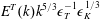 $E^{T}(k)k^{5/3}\unicode[STIX]{x1D716}_{T}^{-1}\unicode[STIX]{x1D716}_{K}^{1/3}$ ; (b)  $E^{s}(k)k^{5/3}\unicode[STIX]{x1D716}_{s}^{-1}\unicode[STIX]{x1D716}_{K}^{1/3}$ .

Figure 5 shows that both the temperature fluctuation spectrum $E^{T}(k)$ and the entropy fluctuation spectrum $E^{s}(k)$ exhibit the $k^{-5/3}$ scaling behaviour in an inertial range of $0.02\leqslant k\unicode[STIX]{x1D702}\leqslant 0.08$ at $M_{t}=0.2$ , 0.6, where $\unicode[STIX]{x1D702}$ is the Kolmogorov length scale. Moreover, the compensated fluctuation spectra of temperature and entropy are nearly constant in the inertial range, i.e. $E^{T}(k)k^{5/3}\unicode[STIX]{x1D716}_{T}^{-1}\unicode[STIX]{x1D716}_{K}^{1/3}\approx C_{T}$ and $E^{s}(k)k^{5/3}\unicode[STIX]{x1D716}_{s}^{-1}\unicode[STIX]{x1D716}_{K}^{1/3}\approx C_{s}$ . The constants $C_{T}=0.60$ and $C_{s}=0.68$ are close to the typical Obukhov–Corrsin constant 0.7 of a passive scalar spectrum (Obukhov Reference Obukhov1949; Corrsin Reference Corrsin1951; Sreenivasan Reference Sreenivasan1996; Yeung, Donzis & Sreenivasan Reference Yeung, Donzis and Sreenivasan2005; Gotoh & Watanabe Reference Gotoh and Watanabe2015). This observation indicates that the fluctuation spectra of both temperature and entropy can be well described by the Obukhov–Corrsin theory of a passive scalar (Obukhov Reference Obukhov1949; Corrsin Reference Corrsin1951).

The compensated spectra of the isentropic and entropic modes of temperature $E^{T,I}(k)k^{5/3}\unicode[STIX]{x1D716}_{T}^{-1}\unicode[STIX]{x1D716}_{K}^{1/3}$ and $E^{T,E}(k)k^{5/3}\unicode[STIX]{x1D716}_{T}^{-1}\unicode[STIX]{x1D716}_{K}^{1/3}$ are plotted in figure 6. It is shown that the spectrum of the entropic mode of temperature is much larger than that of the isentropic mode of temperature at $M_{t}=0.2$ , 0.6. The spectrum of the isentropic mode of temperature decreases rapidly with the decrease of turbulent Mach number, while the spectrum of the entropic mode of temperature increases slightly with the decrease of turbulent Mach number. Moreover, the compensated fluctuation spectrum of the entropic mode of temperature is nearly constant in the inertial range, i.e. $E^{T,E}(k)k^{5/3}\unicode[STIX]{x1D716}_{T}^{-1}\unicode[STIX]{x1D716}_{K}^{1/3}\approx 0.6$ and 0.5 for turbulent Mach numbers $M_{t}=0.2$ and 0.6, respectively.

Figure 6.

Compensated spectra of the isentropic and entropic modes of temperature at $M_{t}=0.2$ , 0.6: (a)  $M_{t}=0.2$ ; (b)  $M_{t}=0.6$ .

Table 3.

Statistics of velocity and its two components in hyperviscosity simulations.

Table 4.

Statistics of thermodynamic variables in hyperviscosity simulations.

The $k^{-5/3}$ scaling behaviours of the spectra of the compressible velocity component, density, pressure, temperature and entropy are observed in our numerical simulations. To further confirm these scaling behaviours, we perform numerical simulations of Euler equations with an eighth-order hyperviscosity (Wang et al. Reference Wang, Wang, Xiao, Shi and Chen2010, Reference Wang, Yang, Shi, Xiao, He and Chen2013), at the same turbulent Mach numbers $M_{t}=0.2$ , 0.6 and at $512^{3}$ grid resolution. Statistics of velocity, solenoidal velocity component, compressible velocity component and thermodynamic variables in hyperviscosity simulations are summarized in tables 3–4. The r.m.s. values of velocity, solenoidal velocity component, compressible velocity component and thermodynamic variables are close to those in the numerical simulations of the Navier–Stokes equations as shown in tables 1–2.

Figure 7.

Normalized spectra of velocity and compressible velocity component at $M_{t}=0.2$ , 0.6 in hyperviscosity simulations: (a)  $E^{u}(k)/(u^{\prime })^{2}$ ; (b)  $E^{u,C}(k)/(u^{\prime })^{2}$ .

Figure 8.

Normalized spectra of density and pressure at $M_{t}=0.2$ , 0.6 in hyperviscosity simulations: (a)  $E^{\unicode[STIX]{x1D70C}}(k)/(\unicode[STIX]{x1D70C}_{rms})^{2}$ ; (b)  $E^{p}(k)/(p_{rms})^{2}$ .

Figure 9.

Normalized spectra of temperature and entropy at $M_{t}=0.2$ , 0.6 in hyperviscosity simulations: (a)  $E^{T}(k)/(T_{rms})^{2}$ ; (b)  $E^{s}(k)/(s_{rms})^{2}$ .

Normalized spectra of the velocity, compressible velocity component, density, pressure, temperature and entropy in the hyperviscosity simulations are plotted in figures 7–9. The spectra exhibit the $k^{-5/3}$ scaling more clearly for a range of $0.02\leqslant k\unicode[STIX]{x1D6E5}\leqslant 0.2$ , as compared to the situation of the numerical simulations of the Navier–Stokes equations. Provided that the inertial-range statistics are independent of the dissipation mechanism (Benzi et al. Reference Benzi, Biferale, Fisher, Kadanoff, Lamb and Toschi2008), the spectra of the velocity and thermodynamic variables will exhibit clearer $k^{-5/3}$ scaling behaviours at higher Reynolds numbers in compressible isotropic turbulence with a heat source by the numerical simulations of the Navier–Stokes equations.

5 Inter-scale transfer of temperature and entropy fluctuations

We apply the Favre filtering approach (Aluie Reference Aluie2011, Reference Aluie2013; Eyink & Drivas Reference Eyink and Drivas2018; Wang et al. Reference Wang, Wan, Chen and Chen2018a ) to study the inter-scale transfer of temperature and entropy. A classically filtered field $\overline{f}$ is defined as $\overline{f}(\boldsymbol{x})=\int \text{d}^{3}\boldsymbol{r}G_{l}(\boldsymbol{r})f(\boldsymbol{x}+\boldsymbol{r})$ . Here, $G_{l}(\boldsymbol{r})=l^{-3}G(\boldsymbol{r}/l)$ is the filter function, $G(\boldsymbol{r})$ is a normalized window function and $l$ is the filter width. The Favre filtered field $\widetilde{f}$ is defined as $\widetilde{f}=\overline{\unicode[STIX]{x1D70C}f}/\overline{\unicode[STIX]{x1D70C}}$ . The equation for the r.m.s. value of the filtered temperature reads:

(5.1) $$\begin{eqnarray}\frac{\unicode[STIX]{x2202}}{\unicode[STIX]{x2202}t}\langle \widetilde{T}_{1}^{2}\rangle =-\langle \unicode[STIX]{x1D6F7}_{l}^{T}+\unicode[STIX]{x1D6F1}_{l}^{T}+D_{l}^{T}+F_{l}^{T}\rangle ,\end{eqnarray}$$

where, $\unicode[STIX]{x1D6F7}_{l}^{T}$ is the dilatation term, $\unicode[STIX]{x1D6F1}_{l}^{T}$ is the subgrid-scale (SGS) term, $D_{l}^{T}$ represents the effect of thermal diffusion and viscous dissipation and $F_{l}^{T}$ represents the effect of large-scale forcing. Here, $\unicode[STIX]{x1D6F7}_{l}^{T}=-(3-2\unicode[STIX]{x1D6FE})\widetilde{T}_{1}^{2}\unicode[STIX]{x1D703}_{l}+2(\unicode[STIX]{x1D6FE}-1)T_{0}\widetilde{T}_{1}\unicode[STIX]{x1D703}_{l}$ , $\unicode[STIX]{x1D703}_{l}=\unicode[STIX]{x2202}\widetilde{u}_{j}/\unicode[STIX]{x2202}x_{j}$ , $\unicode[STIX]{x1D6F1}_{l}^{T}=\unicode[STIX]{x1D6F1}_{l}^{T,1}+\unicode[STIX]{x1D6F1}_{l}^{T,2}$ , $D_{l}^{T}=-2\widetilde{T}_{1}(\widetilde{D_{\unicode[STIX]{x1D705}}}+\widetilde{D_{\unicode[STIX]{x1D707}}})$ and $F_{l}^{T}=-2\widetilde{T}_{1}\widetilde{f_{T}}$ . $\unicode[STIX]{x1D6F1}_{l}^{T,1}=-2[\overline{\unicode[STIX]{x1D70C}}(\widetilde{T_{1}u_{j}}-\widetilde{T}_{1}\widetilde{u}_{j})](\unicode[STIX]{x2202}/\unicode[STIX]{x2202}x_{j})(\widetilde{T}_{1}/\overline{\unicode[STIX]{x1D70C}})$ , and $\unicode[STIX]{x1D6F1}_{l}^{T,2}=2(\unicode[STIX]{x1D6FE}-1)\widetilde{T}_{1}(\widetilde{T_{1}\unicode[STIX]{x1D703}}-\widetilde{T}_{1}\unicode[STIX]{x1D703}_{l})$ . $\unicode[STIX]{x1D6F1}_{l}^{T,1}$ and $\unicode[STIX]{x1D6F1}_{2}^{T,2}$ represent the SGS fluxes induced by the correlation between temperature and velocity, and by the correlation between temperature and velocity divergence, respectively.

The equation for the r.m.s. value of filtered entropy can be written as:

(5.2) $$\begin{eqnarray}\frac{\unicode[STIX]{x2202}}{\unicode[STIX]{x2202}t}\langle \,\widetilde{s}_{1}^{2}\rangle =-\langle \unicode[STIX]{x1D6F7}_{l}^{s}+\unicode[STIX]{x1D6F1}_{l}^{s}+D_{l}^{s}+F_{l}^{s}\rangle ,\end{eqnarray}$$

where, $\unicode[STIX]{x1D6F7}_{l}^{s}$ is the dilatation term, $\unicode[STIX]{x1D6F1}_{l}^{s}$ is the subgrid-scale (SGS) term, $D_{l}^{s}$ represents the effect of thermal diffusion and viscous dissipation and $F_{l}^{s}$ represents the effect of large-scale forcing. Here, $\unicode[STIX]{x1D6F7}_{l}^{s}=-\widetilde{s}_{1}^{2}\unicode[STIX]{x1D703}_{l}$ , $\unicode[STIX]{x1D6F1}_{l}^{s}=-2[\overline{\unicode[STIX]{x1D70C}}(\widetilde{s_{1}u_{j}}-\widetilde{s}_{1}\widetilde{u}_{j})](\unicode[STIX]{x2202}/\unicode[STIX]{x2202}x_{j})(\widetilde{s}_{1}/\overline{\unicode[STIX]{x1D70C}})$ , $D_{l}^{s}=-2\widetilde{s}_{1}(\widetilde{D_{\unicode[STIX]{x1D705}}/T}+\widetilde{D_{\unicode[STIX]{x1D707}}/T})$ , and $F_{l}^{s}=-2\widetilde{s}_{1}\widetilde{f_{T}/T}$ .

We plot spatial average values of $\langle \unicode[STIX]{x1D6F7}_{l}^{T}+\unicode[STIX]{x1D6F1}_{l}^{T}+D_{l}^{T}\rangle /\unicode[STIX]{x1D716}_{T}$ , $\langle \unicode[STIX]{x1D6F7}_{l}^{T}\rangle /\unicode[STIX]{x1D716}_{T}$ , $\langle \unicode[STIX]{x1D6F1}_{l}^{T}\rangle /\unicode[STIX]{x1D716}_{T}$ and $\langle D_{l}^{T}\rangle /\unicode[STIX]{x1D716}_{T}$ at $M_{t}=0.2$ , 0.6 in figure 10. We also plot spatial average values of $\langle \unicode[STIX]{x1D6F7}_{l}^{s}+\unicode[STIX]{x1D6F1}_{l}^{s}+D_{l}^{s}\rangle /\unicode[STIX]{x1D716}_{s}$ , $\langle \unicode[STIX]{x1D6F7}_{l}^{s}\rangle /\unicode[STIX]{x1D716}_{s}$ , $\langle \unicode[STIX]{x1D6F1}_{l}^{s}\rangle /\unicode[STIX]{x1D716}_{s}$ and $\langle D_{l}^{s}\rangle /\unicode[STIX]{x1D716}_{s}$ at $M_{t}=0.2$ , 0.6 in figure 11. The filter width $l$ has been normalized by the Kolmogorov length scale  $\unicode[STIX]{x1D702}$ . It is shown that $\langle \unicode[STIX]{x1D6F7}_{l}^{T}+\unicode[STIX]{x1D6F1}_{l}^{T}+D_{l}^{T}\rangle /\unicode[STIX]{x1D716}_{T}\approx 1$ and $\langle \unicode[STIX]{x1D6F7}_{l}^{s}+\unicode[STIX]{x1D6F1}_{l}^{s}+D_{l}^{s}\rangle /\unicode[STIX]{x1D716}_{s}\approx 1$ for $l/\unicode[STIX]{x1D702}\leqslant 120$ , indicating that the effects of large-scale forcing on inter-scale transfer processes of temperature and entropy fluctuations are localized to the large scales. $\langle \unicode[STIX]{x1D6F1}_{l}^{T}\rangle /\unicode[STIX]{x1D716}_{T}$ and $\langle \unicode[STIX]{x1D6F1}_{l}^{s}\rangle /\unicode[STIX]{x1D716}_{s}$ are nearly constant and are close to 1.0, over an inertial range $30\leqslant l/\unicode[STIX]{x1D702}\leqslant 120$ . Moreover, $\langle \unicode[STIX]{x1D6F1}_{l}^{T}\rangle /\unicode[STIX]{x1D716}_{T}$ and $\langle \unicode[STIX]{x1D6F1}_{l}^{s}\rangle /\unicode[STIX]{x1D716}_{s}$ decrease slightly with the increase of turbulent Mach number. It is found that terms $\langle \unicode[STIX]{x1D6F7}_{l}^{T}\rangle$ , $\langle D_{l}^{T}\rangle$ , $\langle F_{l}^{T}\rangle$ , $\langle \unicode[STIX]{x1D6F7}_{l}^{s}\rangle$ , $\langle D_{l}^{s}\rangle$ and $\langle F_{l}^{s}\rangle$ are small in the inertial range. It is also found that $\langle \unicode[STIX]{x1D6F1}_{l}^{T,1}\rangle /\unicode[STIX]{x1D716}_{T}$ is much larger than $\langle \unicode[STIX]{x1D6F1}_{l}^{T,2}\rangle /\unicode[STIX]{x1D716}_{T}$ . These observations indicate the existence of direct cascades of temperature and entropy fluctuations from large scales to small scales through the inertial range.

Figure 10.

Average values of $\langle \unicode[STIX]{x1D6F7}_{l}^{T}+\unicode[STIX]{x1D6F1}_{l}^{T}+D_{l}^{T}\rangle /\unicode[STIX]{x1D716}_{T}$ , $\langle \unicode[STIX]{x1D6F7}_{l}^{T}\rangle /\unicode[STIX]{x1D716}_{T}$ , $\langle \unicode[STIX]{x1D6F1}_{l}^{T}\rangle /\unicode[STIX]{x1D716}_{T}$ and $\langle D_{l}^{T}\rangle /\unicode[STIX]{x1D716}_{T}$ at $M_{t}=0.2$ , 0.6: (a)  $M_{t}=0.2$ ; (b)  $M_{t}=0.6$ .

Figure 11.

Average values of $\langle \unicode[STIX]{x1D6F7}_{l}^{s}+\unicode[STIX]{x1D6F1}_{l}^{s}+D_{l}^{s}\rangle /\unicode[STIX]{x1D716}_{s}$ , $\langle \unicode[STIX]{x1D6F7}_{l}^{s}\rangle /\unicode[STIX]{x1D716}_{s}$ , $\langle \unicode[STIX]{x1D6F1}_{l}^{s}\rangle /\unicode[STIX]{x1D716}_{s}$ and $\langle D_{l}^{s}\rangle /\unicode[STIX]{x1D716}_{s}$ at $M_{t}=0.2$ , 0.6: (a)  $M_{t}=0.2$ ; (b)  $M_{t}=0.6$ .

The SGS fluxes of temperature due to the solenoidal and compressible modes of the velocity are, respectively,

(5.3) $$\begin{eqnarray}\unicode[STIX]{x1D6F1}_{l}^{T,S}=-2\left[\overline{\unicode[STIX]{x1D70C}}(\widetilde{T_{1}u_{j}^{S}}-\widetilde{T}_{1}\widetilde{u}_{j}^{S})\right]\frac{\unicode[STIX]{x2202}}{\unicode[STIX]{x2202}x_{j}}\left(\frac{\widetilde{T}_{1}}{\overline{\unicode[STIX]{x1D70C}}}\right),\end{eqnarray}$$

and,

(5.4) $$\begin{eqnarray}\unicode[STIX]{x1D6F1}_{l}^{T,C}=-2\left[\overline{\unicode[STIX]{x1D70C}}(\widetilde{T_{1}u_{j}^{C}}-\widetilde{T}_{1}\widetilde{u}_{j}^{C})\right]\frac{\unicode[STIX]{x2202}}{\unicode[STIX]{x2202}x_{j}}\left(\frac{\widetilde{T}_{1}}{\overline{\unicode[STIX]{x1D70C}}}\right)+\unicode[STIX]{x1D6F1}_{l}^{T,2}.\end{eqnarray}$$

Similarly, the SGS fluxes of entropy due to the solenoidal and compressible modes of the velocity are, respectively,

(5.5) $$\begin{eqnarray}\unicode[STIX]{x1D6F1}_{l}^{s,S}=-2\left[\overline{\unicode[STIX]{x1D70C}}(\widetilde{s_{1}u_{j}^{S}}-\widetilde{s}_{1}\widetilde{u}_{j}^{S})\right]\frac{\unicode[STIX]{x2202}}{\unicode[STIX]{x2202}x_{j}}\left(\frac{\widetilde{s}_{1}}{\overline{\unicode[STIX]{x1D70C}}}\right),\end{eqnarray}$$

and,

(5.6) $$\begin{eqnarray}\unicode[STIX]{x1D6F1}_{l}^{s,C}=-2\left[\overline{\unicode[STIX]{x1D70C}}(\widetilde{s_{1}u_{j}^{C}}-\widetilde{s}_{1}\widetilde{u}_{j}^{C})\right]\frac{\unicode[STIX]{x2202}}{\unicode[STIX]{x2202}x_{j}}\left(\frac{\widetilde{s}_{1}}{\overline{\unicode[STIX]{x1D70C}}}\right).\end{eqnarray}$$

Here, $\widetilde{\boldsymbol{u}}^{S}$ and $\widetilde{\boldsymbol{u}}^{C}$ are the solenoidal and compressible components of the filtered velocity field $\widetilde{\boldsymbol{u}}$ , respectively.

We plot spatial average values of SGS fluxes of temperature and entropy due to the solenoidal and compressible modes of velocity at $M_{t}=0.2$ , 0.6 in figure 12. It is found that $\langle \unicode[STIX]{x1D6F1}_{l}^{T,S}\rangle /\unicode[STIX]{x1D716}_{T}\approx 0$ and $\langle \unicode[STIX]{x1D6F1}_{l}^{s,C}\rangle /\unicode[STIX]{x1D716}_{s}\approx 0$ , namely, $\langle \unicode[STIX]{x1D6F1}_{l}^{T,C}\rangle /\unicode[STIX]{x1D716}_{T}\approx \langle \unicode[STIX]{x1D6F1}_{l}^{T}\rangle /\unicode[STIX]{x1D716}_{T}$ and $\langle \unicode[STIX]{x1D6F1}_{l}^{s,S}\rangle /\unicode[STIX]{x1D716}_{s}\approx \langle \unicode[STIX]{x1D6F1}_{l}^{s}\rangle /\unicode[STIX]{x1D716}_{s}$ . Thus, the average SGS flux of temperature is dominated by the compressible mode of the velocity field, indicating that the theory of a passive scalar in incompressible turbulence, which was often used for the temperature field in compressible turbulence, is not suitable to describe the inter-scale transfer of temperature in compressible turbulence. The average SGS flux of entropy is dominated by the solenoidal mode of the velocity field, which is similar to that of a passive scalar in incompressible turbulence.

Figure 12.

Average values of SGS fluxes of temperature and entropy due to the solenoidal and compressible modes of velocity at $M_{t}=0.2$ , 0.6: (a)  $\langle \unicode[STIX]{x1D6F1}_{l}^{T,S}\rangle /\unicode[STIX]{x1D716}_{T}$ and $\langle \unicode[STIX]{x1D6F1}_{l}^{T,C}\rangle /\unicode[STIX]{x1D716}_{T}$ ; (b)  $\langle \unicode[STIX]{x1D6F1}_{l}^{s,S}\rangle /\unicode[STIX]{x1D716}_{s}$ and $\langle \unicode[STIX]{x1D6F1}_{l}^{s,C}\rangle /\unicode[STIX]{x1D716}_{s}$ .

Figure 13.

PDFs of SGS fluxes of temperature and entropy for $l/\unicode[STIX]{x1D702}=16$ , 32, 64 at $M_{t}=0.2$ , 0.6: (a) PDFs of $\unicode[STIX]{x1D6F1}_{l}^{T}/\unicode[STIX]{x1D716}_{T}$ at $M_{t}=0.2$ ; (b) PDFs of $\unicode[STIX]{x1D6F1}_{l}^{s}/\unicode[STIX]{x1D716}_{s}$ at $M_{t}=0.2$ ; (c) PDFs of $\unicode[STIX]{x1D6F1}_{l}^{T}/\unicode[STIX]{x1D716}_{T}$ at $M_{t}=0.6$ ; (d) PDFs of $\unicode[STIX]{x1D6F1}_{l}^{s}/\unicode[STIX]{x1D716}_{s}$ at $M_{t}=0.6$ .

The probability density functions (PDFs) of the SGS fluxes of temperature and entropy for $l/\unicode[STIX]{x1D702}=16$ , 32, 64 at $M_{t}=0.2$ , 0.6 are depicted in figure 13. It is shown that the PDFs of SGS fluxes exhibit a skewness toward the positive side, suggesting that the SGS fluxes of temperature and entropy have a tendency to direct from large scales to small scales. The tails of PDFs become longer as the filter width $l$ decreases. The tails of PDFs of $\unicode[STIX]{x1D6F1}_{l}^{T}/\unicode[STIX]{x1D716}_{T}$ are slightly shorter than those of $\unicode[STIX]{x1D6F1}_{l}^{s}/\unicode[STIX]{x1D716}_{s}$ at $M_{t}=0.2$ . As turbulent Mach number increases to $M_{t}=0.6$ , the tails of PDFs of $\unicode[STIX]{x1D6F1}_{l}^{T}/\unicode[STIX]{x1D716}_{T}$ become longer while the tails of PDFs of $\unicode[STIX]{x1D6F1}_{l}^{s}/\unicode[STIX]{x1D716}_{s}$ become shorter. This observation indicates that the extremely high magnitude of the SGS temperature flux is enhanced and the extremely high magnitude of the SGS entropy flux is suppressed with the increase of turbulent Mach number. The tails of the PDFs of $\unicode[STIX]{x1D6F1}_{l}^{T}/\unicode[STIX]{x1D716}_{T}$ are significantly longer than those of $\unicode[STIX]{x1D6F1}_{l}^{s}/\unicode[STIX]{x1D716}_{s}$ at $M_{t}=0.6$ .

Figure 14.

PDFs of SGS fluxes of temperature and entropy due to two components of the velocity for $l/\unicode[STIX]{x1D702}=16$ at $M_{t}=0.2$ , 0.6: (a) PDFs of $\unicode[STIX]{x1D6F1}_{l}^{T,C}/\unicode[STIX]{x1D716}_{T}$ and $\unicode[STIX]{x1D6F1}_{l}^{T,S}/\unicode[STIX]{x1D716}_{T}$ at $M_{t}=0.2$ ; (b) PDFs of $\unicode[STIX]{x1D6F1}_{l}^{s,S}/\unicode[STIX]{x1D716}_{s}$ and $\unicode[STIX]{x1D6F1}_{l}^{s,C}/\unicode[STIX]{x1D716}_{s}$ at $M_{t}=0.2$ ; (c) PDFs of $\unicode[STIX]{x1D6F1}_{l}^{T,C}/\unicode[STIX]{x1D716}_{T}$ and $\unicode[STIX]{x1D6F1}_{l}^{T,S}/\unicode[STIX]{x1D716}_{T}$ at $M_{t}=0.6$ ; (d) PDFs of $\unicode[STIX]{x1D6F1}_{l}^{s,S}/\unicode[STIX]{x1D716}_{s}$ and $\unicode[STIX]{x1D6F1}_{l}^{s,C}/\unicode[STIX]{x1D716}_{s}$ at $M_{t}=0.6$ .

Figure 14 shows the PDFs of the SGS fluxes of temperature and entropy due to two components of the velocity for $l/\unicode[STIX]{x1D702}=16$ at $M_{t}=0.2$ , 0.6. It is found that the PDF of  $\unicode[STIX]{x1D6F1}_{l}^{T,C}/\unicode[STIX]{x1D716}_{T}$ is similar to that of $\unicode[STIX]{x1D6F1}_{l}^{T}/\unicode[STIX]{x1D716}_{T}$ , which is consistent with the previous observation that the average SGS flux of temperature is dominated by the compressible velocity component. The right tail of the PDF of $\unicode[STIX]{x1D6F1}_{l}^{T,S}/\unicode[STIX]{x1D716}_{T}$ is significantly shorter than that of $\unicode[STIX]{x1D6F1}_{l}^{T,C}/\unicode[STIX]{x1D716}_{T}$ , implying that the contribution of the solenoidal velocity component to the average SGS temperature flux is significantly smaller than that of the compressible velocity component. Similarly, the PDF of $\unicode[STIX]{x1D6F1}_{l}^{s,S}/\unicode[STIX]{x1D716}_{s}$ is similar to that of $\unicode[STIX]{x1D6F1}_{l}^{s}/\unicode[STIX]{x1D716}_{s}$ , giving rise to the fact that the average SGS flux of entropy is dominated by the solenoidal velocity component. The right tail of the PDF of $\unicode[STIX]{x1D6F1}_{l}^{s,C}/\unicode[STIX]{x1D716}_{T}$ is much shorter than that of $\unicode[STIX]{x1D6F1}_{l}^{s,S}/\unicode[STIX]{x1D716}_{T}$ , suggesting that the contribution of the compressible velocity component to the average SGS entropy flux is much smaller than that of the solenoidal velocity component.

Now we define the following geometrical variables for the SGS fluxes of temperature and entropy: $\unicode[STIX]{x1D719}_{l}^{T}=\boldsymbol{Q}^{T}\boldsymbol{\cdot }\boldsymbol{G}^{T}/(|\boldsymbol{Q}^{T}|\,|\boldsymbol{G}^{T}|)$ , and $\unicode[STIX]{x1D719}_{l}^{s}=\boldsymbol{Q}^{s}\boldsymbol{\cdot }\boldsymbol{G}^{s}/(|\boldsymbol{Q}^{s}|\,|\boldsymbol{G}^{s}|)$ , where $Q_{j}^{T}=\overline{\unicode[STIX]{x1D70C}}(\widetilde{T_{1}u_{j}}-\widetilde{T}_{1}\widetilde{u}_{j})$ , $G_{j}^{T}=(\unicode[STIX]{x2202}/\unicode[STIX]{x2202}x_{j})(\widetilde{T}_{1}/\overline{\unicode[STIX]{x1D70C}})$ , $Q_{j}^{s}=\overline{\unicode[STIX]{x1D70C}}(\widetilde{s_{1}u_{j}}-\widetilde{s}_{1}\widetilde{u}_{j})$ and $G_{j}^{s}=(\unicode[STIX]{x2202}/\unicode[STIX]{x2202}x_{j})(\widetilde{s}_{1}/\overline{\unicode[STIX]{x1D70C}})$ . Similarly, we can define the geometrical variables for SGS fluxes of temperature and entropy due to two components of the velocity as follows: $\unicode[STIX]{x1D719}_{l}^{T,X}=\boldsymbol{Q}^{T,X}\boldsymbol{\cdot }\boldsymbol{G}^{T}/(|\boldsymbol{Q}^{T,X}|\,|\boldsymbol{G}^{T}|)$ , and $\unicode[STIX]{x1D719}_{l}^{s,X}=\boldsymbol{Q}^{s,X}\boldsymbol{\cdot }\boldsymbol{G}^{s}/(|\boldsymbol{Q}^{s,X}|\,|\boldsymbol{G}^{s}|)$ , where $Q_{j}^{T,X}=\overline{\unicode[STIX]{x1D70C}}(\widetilde{T_{1}u_{j}^{X}}-\widetilde{T}_{1}\widetilde{u}_{j}^{X})$ , $Q_{j}^{s,X}=\overline{\unicode[STIX]{x1D70C}}(\widetilde{s_{1}u_{j}^{X}}-\widetilde{s}_{1}\widetilde{u}_{j}^{X})$ and $X=S$ , $C$ . We plot the PDFs of $\unicode[STIX]{x1D719}_{l}^{T}$ , $\unicode[STIX]{x1D719}_{l}^{T,S}$ , $\unicode[STIX]{x1D719}_{l}^{T,C}$ , $\unicode[STIX]{x1D719}_{l}^{s}$ , $\unicode[STIX]{x1D719}_{l}^{s,S}$ and $\unicode[STIX]{x1D719}_{l}^{s,C}$ at $M_{t}=0.2$ , 0.6 in figure 15. Both geometrical variables $\unicode[STIX]{x1D719}_{l}^{T}$ and $\unicode[STIX]{x1D719}_{l}^{s}$ have a tendency to be negative, in agreement with the overall direct cascade of temperature and entropy from large scales to small scales. It is found that the geometrical variable $\unicode[STIX]{x1D719}_{l}^{T,C}$ has a tendency to be $-1$ , while the PDF of geometrical variable $\unicode[STIX]{x1D719}_{l}^{T,S}$ is nearly symmetrical with respect to $\unicode[STIX]{x1D719}_{l}^{T,S}=0$ . This observation partly explains why the cascade of temperature is dominated by the compressible mode of the velocity field. In contrast, the PDF of the geometrical variable $\unicode[STIX]{x1D719}_{l}^{s,C}$ is nearly symmetrical with respect to $\unicode[STIX]{x1D719}_{l}^{s,C}=0$ , while the PDF of the geometrical variable $\unicode[STIX]{x1D719}_{l}^{s,S}$ is almost identical to that of  $\unicode[STIX]{x1D719}_{l}^{s}$ . The observation is consistent with the fact that the cascade of entropy is dominated by the solenoidal mode of the velocity field. The effect of turbulent Mach number on the statistics of the geometrical variables is negligibly small.

Figure 15.

PDFs of geometrical variables for SGS fluxes of temperature and entropy, and their compressible and solenoidal components at $M_{t}=0.2$ , 0.6: (a) PDFs of $\unicode[STIX]{x1D719}_{l}^{T}$ , $\unicode[STIX]{x1D719}_{l}^{T,S}$ and $\unicode[STIX]{x1D719}_{l}^{T,C}$ at $M_{t}=0.2$ ; (b) PDFs of $\unicode[STIX]{x1D719}_{l}^{s}$ , $\unicode[STIX]{x1D719}_{l}^{s,S}$ and $\unicode[STIX]{x1D719}_{l}^{s,C}$ at $M_{t}=0.2$ ; (c) PDFs of $\unicode[STIX]{x1D719}_{l}^{T}$ , $\unicode[STIX]{x1D719}_{l}^{T,S}$ and $\unicode[STIX]{x1D719}_{l}^{T,C}$ at $M_{t}=0.6$ ; (d) PDFs of $\unicode[STIX]{x1D719}_{l}^{s}$ , $\unicode[STIX]{x1D719}_{l}^{s,S}$ and $\unicode[STIX]{x1D719}_{l}^{s,C}$ at $M_{t}=0.6$ .

To clarify the impact of local compression and expansion motions on the inter-scale transfer of temperature and entropy, we plot the average of SGS fluxes of temperature and entropy conditioned on the normalized filtered dilatation $\unicode[STIX]{x1D703}_{l}/\unicode[STIX]{x1D703}_{l}^{\prime }$ for $l/\unicode[STIX]{x1D702}=16$ at $M_{t}=0.2$ , 0.6 in figure 16. Here, $\unicode[STIX]{x1D703}_{l}^{\prime }=\sqrt{\langle \unicode[STIX]{x1D703}_{l}^{2}\rangle }$ is the r.m.s. value of the filtered dilatation. The fluctuations of the conditional average curves for $\unicode[STIX]{x1D703}_{l}/\unicode[STIX]{x1D703}_{l}^{\prime }>6$ are due to the lack of samples. It is shown that the conditional average SGS fluxes $\langle \unicode[STIX]{x1D6F1}_{l}^{T}/\unicode[STIX]{x1D716}_{T}\,|\,\unicode[STIX]{x1D703}_{l}/\unicode[STIX]{x1D703}_{l}^{\prime }\rangle$ and $\langle \unicode[STIX]{x1D6F1}_{l}^{s}/\unicode[STIX]{x1D716}_{s}\,|\,\unicode[STIX]{x1D703}_{l}/\unicode[STIX]{x1D703}_{l}^{\prime }\rangle$ increase with the increase of magnitude of the filtered dilatation in compression regions $\unicode[STIX]{x1D703}_{l}/\unicode[STIX]{x1D703}_{l}^{\prime }<0$ , and decrease with the increase of magnitude of the filtered dilatation in expansion regions $\unicode[STIX]{x1D703}_{l}/\unicode[STIX]{x1D703}_{l}^{\prime }>0$ . The observation indicates that compression motions enhance the direct SGS flux of temperature and entropy, while expansion motions suppress the direct SGS flux of temperature and entropy. Moreover, $\langle \unicode[STIX]{x1D6F1}_{l}^{T}/\unicode[STIX]{x1D716}_{T}\,|\,\unicode[STIX]{x1D703}_{l}/\unicode[STIX]{x1D703}_{l}^{\prime }\rangle$ becomes negative for $\unicode[STIX]{x1D703}_{l}/\unicode[STIX]{x1D703}_{l}^{\prime }>5$ , giving rise to the reverse SGS flux of temperature from small scales to large scales in very strong expansion regions. It is worth noting that the magnitude of the conditional average SGS flux of the temperature in strong compression regions is much higher than that in strong expansion regions, demonstrating that the effect of compression motions on the inter-scale transfer of temperature is significantly larger than that of expansion motions. Moreover, the effect of compressibility on the inter-scale transfer of temperature is much stronger than on the inter-scale transfer of entropy, due to the explicit effect of velocity divergence term in the dynamical equation of temperature.

Figure 16.

Conditional average SGS fluxes of temperature and entropy, and their compressible and solenoidal components for $l/\unicode[STIX]{x1D702}=16$ at $M_{t}=0.2$ , 0.6: (a)  $\langle \unicode[STIX]{x1D6F1}_{l}^{T}/\unicode[STIX]{x1D716}_{T}\,|\,\unicode[STIX]{x1D703}_{l}/\unicode[STIX]{x1D703}_{l}^{\prime }\rangle$ , $\langle \unicode[STIX]{x1D6F1}_{l}^{T,S}/\unicode[STIX]{x1D716}_{T}\,|\,\unicode[STIX]{x1D703}_{l}/\unicode[STIX]{x1D703}_{l}^{\prime }\rangle$ and $\langle \unicode[STIX]{x1D6F1}_{l}^{T,C}/\unicode[STIX]{x1D716}_{T}\,|\,\unicode[STIX]{x1D703}_{l}/\unicode[STIX]{x1D703}_{l}^{\prime }\rangle$ at $M_{t}=0.2$ ; (b)  $\langle \unicode[STIX]{x1D6F1}_{l}^{s}/\unicode[STIX]{x1D716}_{s}\,|\,\unicode[STIX]{x1D703}_{l}/\unicode[STIX]{x1D703}_{l}^{\prime }\rangle$ , $\langle \unicode[STIX]{x1D6F1}_{l}^{s,S}/\unicode[STIX]{x1D716}_{s}\,|\,\unicode[STIX]{x1D703}_{l}/\unicode[STIX]{x1D703}_{l}^{\prime }\rangle$ and $\langle \unicode[STIX]{x1D6F1}_{l}^{s,C}/\unicode[STIX]{x1D716}_{s}\,|\,\unicode[STIX]{x1D703}_{l}/\unicode[STIX]{x1D703}_{l}^{\prime }\rangle$ at $M_{t}=0.2$ ; (c)  $\langle \unicode[STIX]{x1D6F1}_{l}^{T}/\unicode[STIX]{x1D716}_{T}\,|\,\unicode[STIX]{x1D703}_{l}/\unicode[STIX]{x1D703}_{l}^{\prime }\rangle$ , $\langle \unicode[STIX]{x1D6F1}_{l}^{T,S}/\unicode[STIX]{x1D716}_{T}\,|\,\unicode[STIX]{x1D703}_{l}/\unicode[STIX]{x1D703}_{l}^{\prime }\rangle$ and $\langle \unicode[STIX]{x1D6F1}_{l}^{T,C}/\unicode[STIX]{x1D716}_{T}\,|\,\unicode[STIX]{x1D703}_{l}/\unicode[STIX]{x1D703}_{l}^{\prime }\rangle$ at $M_{t}=0.6$ ; (d)  $\langle \unicode[STIX]{x1D6F1}_{l}^{s}/\unicode[STIX]{x1D716}_{s}\,|\,\unicode[STIX]{x1D703}_{l}/\unicode[STIX]{x1D703}_{l}^{\prime }\rangle$ , $\langle \unicode[STIX]{x1D6F1}_{l}^{s,S}/\unicode[STIX]{x1D716}_{s}\,|\,\unicode[STIX]{x1D703}_{l}/\unicode[STIX]{x1D703}_{l}^{\prime }\rangle$ and $\langle \unicode[STIX]{x1D6F1}_{l}^{s,C}/\unicode[STIX]{x1D716}_{s}\,|\,\unicode[STIX]{x1D703}_{l}/\unicode[STIX]{x1D703}_{l}^{\prime }\rangle$ at $M_{t}=0.6$ .

It is interesting to see that the conditional average $\langle \unicode[STIX]{x1D6F1}_{l}^{T,S}/\unicode[STIX]{x1D716}_{T}\,|\,\unicode[STIX]{x1D703}_{l}/\unicode[STIX]{x1D703}_{l}^{\prime }\rangle$ decreases with the increase of magnitude of the filtered dilatation in compression regions, and increases with the increase of magnitude of the filtered dilatation in expansion regions. The local compressibility effect on the SGS temperature flux due to the solenoidal velocity component $\unicode[STIX]{x1D6F1}_{l}^{T,S}$ is opposite to the local compressibility effect on the overall SGS temperature flux  $\unicode[STIX]{x1D6F1}_{l}^{T}$ . It is shown that the conditional average of the SGS temperature flux due to the compressible velocity component $\unicode[STIX]{x1D6F1}_{l}^{T,C}$ is similar to the conditional average of the overall SGS temperature flux  $\unicode[STIX]{x1D6F1}_{l}^{T}$ . In addition, the magnitude of the conditional average of the SGS temperature flux due to the compressible velocity component is much larger than that of the SGS temperature flux due to the solenoidal velocity component in strong compression regions.

It is found that the conditional average $\langle \unicode[STIX]{x1D6F1}_{l}^{s,S}/\unicode[STIX]{x1D716}_{T}\,|\,\unicode[STIX]{x1D703}_{l}/\unicode[STIX]{x1D703}_{l}^{\prime }\rangle$ is close to 1.0 and is insensitive to the change of filtered dilatation, implying that the effect of local compressibility on the SGS entropy flux due to the solenoidal velocity component $\unicode[STIX]{x1D6F1}_{l}^{s,S}$ is very weak. In compression regions, the conditional average $\langle \unicode[STIX]{x1D6F1}_{l}^{s,C}/\unicode[STIX]{x1D716}_{T}\,|\,\unicode[STIX]{x1D703}_{l}/\unicode[STIX]{x1D703}_{l}^{\prime }\rangle$ is positive, and increases with the increase of magnitude of the filtered dilatation. In expansion regions, the conditional average $\langle \unicode[STIX]{x1D6F1}_{l}^{s,C}/\unicode[STIX]{x1D716}_{T}\,|\,\unicode[STIX]{x1D703}_{l}/\unicode[STIX]{x1D703}_{l}^{\prime }\rangle$ is negative, and decreases with the increase of magnitude of filtered dilatation. The observation suggests that compression motions induce the direct SGS entropy flux due to the compressible velocity component $\unicode[STIX]{x1D6F1}_{l}^{s,C}$ from large scales to small scales, which is balanced by the reverse SGS entropy flux due to the compressible velocity component $\unicode[STIX]{x1D6F1}_{l}^{s,C}$ from small scales to large scales induced by expansion motions.