Introduction
The largest climatic warming in the Southern Hemisphere is observed in the region of the Antarctic Peninsula (AP) during the winter months. This was clearly demonstrated by meteorological observations at the Faraday/Vernadsky station (British/Ukrainian station before/after 1996; 65°S, 64°W) that continue since the middle of the last century. The winter temperature trend here was 1.1°C per decade with a general temperature increase of c. 6°C to the early 2000s (Vaughan et al. Reference Vaughan, Marshall, Connolley, Parkinson, Mulvaney, Hodgson, King, Pudsey and Turner2003, Roscoe et al. Reference Roscoe, Marshall and King2006). In the same period, the summer trend was only of 0.2–0.3°C per decade. For comparison, the assessments of the annual mean global warming reveal a trend value of 0.13°C per decade in 1956–2005 (Solomon et al. Reference Solomon, Qin, Manning, Marquis, Averyt, Tignor, Miller and Chen2007). In the context of a relationship between regional and global warming, the AP region is of the same importance as that observed for high latitude North America and Siberia in the Northern Hemisphere (e.g. Turner & Overland Reference Turner and Overland2009).
In the high southern latitudes, the Antarctic Peninsula, with an average width of 70 km and a mean height of 1500 m, forms a climatic barrier that has a major influence on oceanic and atmospheric circulation (e.g. Schwerdtfeger Reference Schwerdtfeger1975, Convey et al. Reference Convey, Bindschadler, Di Prisco, Fahrbach, Gutt, Hodgson, Mayewski, Summerhayes and Turner2009). Climate changes in this region show strong spatial differentiation, especially in the winter season. The west coast of AP in winter is generally 7–10°C warmer than at similar latitudes and elevations on the east coast (Schwerdtfeger Reference Schwerdtfeger1975, Morris & Vaughan Reference Morris and Vaughan1994) and the warming tendency is most evident in the western AP region (Vaughan et al. Reference Vaughan, Marshall, Connolley, Parkinson, Mulvaney, Hodgson, King, Pudsey and Turner2003, Turner et al. Reference Turner, Colwell, Marshall, Lachlan-Cope, Carleton, Jones, Lagun, Reid and Iagovkina2005).
Due to the high warming rate, winter temperatures make the largest contribution to the annual mean temperature increase in the AP region. However, the mechanism underlying rapid regional warming here, and the changing nature of the temperature trends with the annual mean temperature variability on the decadal timescale (Vaughan et al. Reference Vaughan, Marshall, Connolley, Parkinson, Mulvaney, Hodgson, King, Pudsey and Turner2003, Turner et al. Reference Turner, Colwell, Marshall, Lachlan-Cope, Carleton, Jones, Lagun, Reid and Iagovkina2005), are not fully understood at present. In view of the fact that the winter temperatures are of the greatest importance in discussions of AP climate change, we focus on their decadal variability and use Fourier and wavelet analyses to estimate the spectra of temperature oscillations. The long-term temperature changes in the AP region were studied with increasing time series length (e.g. Schwerdtfeger Reference Schwerdtfeger1975, Sansom Reference Sansom1989, King Reference King1994, Vaughan et al. Reference Vaughan, Marshall, Connolley, Parkinson, Mulvaney, Hodgson, King, Pudsey and Turner2003, Turner et al. Reference Turner, Colwell, Marshall, Lachlan-Cope, Carleton, Jones, Lagun, Reid and Iagovkina2005, Zazulie et al. Reference Zazulie, Rusticucci and Solomon2010). We analysed the 1950–2009 period and considered the averaged temperature anomalies for the eight stations of the AP region. The grounds for the regional-scale analysis in this work were a well-known high correlation between the temperature time series recorded in the AP region (King Reference King1994, Vaughan et al. Reference Vaughan, Marshall, Connolley, Parkinson, Mulvaney, Hodgson, King, Pudsey and Turner2003, Ferron et al. Reference Ferron, Simões, Aquino and Setzer2004), as well as the lack of a separate analysis aimed at evaluating decadal changes in the winter temperature in this region.
Data and analysis
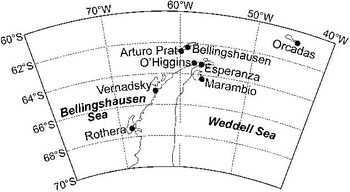
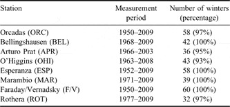
The geographical location of the eight stations chosen for this study is shown in Fig. 1. The AP region under consideration extends c. 1300 km from south-west (Rothera) to north-east (Orcadas Station). The monthly mean temperatures for the 1950–2009 period were taken from the Scientific Committee on Antarctic Research (SCAR) Reference Antarctic Data for Environmental Research (READER). The SCAR READER project is described in detail by Turner et al. (Reference Turner, Colwell, Marshall, Lachlan-Cope, Carleton, Jones, Lagun, Reid and Iagovkina2004). The database of the meteorological parameters (Met READER) is available at http://www.antarctica.ac.uk/met/READER/ (accessed August 2010). Table I contains the measurement periods and the winter data availability in the Met READER database (the second column and the third column, respectively). Mean winter temperatures were calculated by averaging the monthly mean values for the three calendar months of the winter: June, July and August. The data available for two or three winter months were taken into account and winters presented by one month data only were eliminated from the analysis.
Antarctic stations in the region of the Antarctic Peninsula (black circles) chosen for analysis of winter temperatures (see list in Table I).

Availability of winter temperature from the Met READER data over the 1950–2009 period for the eight stations in the Antarctic Peninsula region.
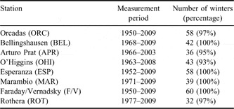
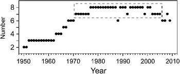
As seen from Table I, the winter temperatures in the Met READER data are presented by the time series of different lengths and some of them are incomplete (93–97% for four stations). Full statistics concerning the number of the stations with available winter data is presented in Fig. 2. The winter data collection is the most complete between the early 1970s and the early 2000s (seven to eight stations, except for 1988 when data was from only six stations; marked by dashed rectangle in Fig. 2).
Data availability (number of stations) of the winter temperatures over the period 1950–2009.

As noted in the previous section, a high correlation exists among the winter temperature time series recorded at different stations in the AP region. It is usually associated with a similarity in the sea ice and atmospheric circulation changes. The correlation coefficients, r, between the eight detrended time series are shown in Table II. The correlation significance was estimated with a Student's t-test accounting for the lag-1 autocorrelation of the individual time series. Because the autocorrelation increase leads to a decrease in the number of the effectively independent observations, the effective sample size (Neff) was calculated as:

where N is the sample size and r 1 and r 2 are the lag-1 autocorrelations of the two time series being correlated (e.g. Ciasto & Thompson Reference Ciasto and Thompson2008).
It is seen from Table II that the correlation coefficients (r) are typically around 0.6–0.7 for the remote stations and are greater than 0.7 for the neighbouring stations. The significance level is less than 1%. The results of Table II agree with the earlier estimates for the shorter time series (King Reference King1994, Vaughan et al. Reference Vaughan, Marshall, Connolley, Parkinson, Mulvaney, Hodgson, King, Pudsey and Turner2003, Ferron et al. Reference Ferron, Simões, Aquino and Setzer2004). Note that detrending the time series does not change appreciably both the r values and their significance level. The conclusion that there is a high spatial coherence in the winter temperature variability over the AP region was made also by the satellite derived surface temperatures for the 1982–2000 period (King & Comiso Reference King and Comiso2003). Hence, a combination of the eight station records can be used to characterize the range and degree of the winter temperature variability on the scale of the AP region, in spite of some incompleteness of the time series used (Table I & Fig. 2).
Correlations (r) between the detrended time series of the winter temperature recorded at the eight stations of the Antarctic Peninsula region during the 1950–2009 period. The 95% confidence intervals with the lag-1 autocorrelation are shown (see the first column in Table I for the abbreviated station names).

The averaged time series analysed in the next section has been created from the temperature anomalies calculated for each station by subtraction of the mean winter temperature. The common 30 year base period 1972–2001 was chosen for the winter means owing to the maximum data completeness (Fig. 2). The standardized version of the averaged time series was used for the Fourier and wavelet transforms. It was obtained by dividing the detrended individual anomaly time series by the base period standard deviation before averaging.
The Fast Fourier transform and wavelet transform were applied for spectral analysis in this work. The statistical significance of spectral peaks was estimated using the red noise background spectrum with a lag-1 autocorrelation (Torrence & Compo Reference Torrence and Compo1998). The wavelet transform is used for analysing the localized variations within a time series to determine the dominant modes of variability and how those modes vary in time (Torrence & Compo Reference Torrence and Compo1998). The continuous wavelet transform with the Morlet function was used. Because the wavelet function is in general complex, the transform can be divided into the real part and imaginary part. The real part of the Morlet wavelet captures both the positive and negative oscillations of the time series and can be used to isolate the separate peaks or discontinuities. In a complex form, the Morlet wavelet combines the positive and negative peaks into a single broad peak that is better for capturing oscillatory behaviour (Torrence & Compo Reference Torrence and Compo1998). In this work, the Morlet 6 function is used.
The linear temperature trend was estimated by a standard least squares method. As with a correlation, the significance level was calculated using the lag-1 autocorrelation coefficient r 1 to determine the effective sample size as described in Eq. (1) but in consideration of the single time series.
For the coldest and warmest winters in the AP region, the sea ice and temperature fields were compared. The monthly mean sea ice concentrations were obtained from the National Snow and Ice Data Center (NSIDC) at ftp://sidads.colorado.edu/pub/DATASETS/nsidc0051_gsfc_nasateam_seaice/ (accessed February 2010; Cavalieri et al. Reference Cavalieri, Parkinson, Gloersen and Zwally1996). The winter temperatures (June–August) for the 1000 hPa pressure level from the National Centers of Environmental Prediction Reanalysis-2 (NCEP R-2) data at http://www.esrl.noaa.gov/psd/data/gridded/data.ncep.reanalysis2.html (accessed December 2009; Kanamitsu et al. Reference Kanamitsu, Ebisuzaki, Woollen, Yang, Hnilo, Fiorino and Potter2002) were used. Besides, the averaged time series of the winter temperature anomalies was correlated with the Southern Annular Mode (SAM) index developed by G.J. Marshall and available at http://www.antarctica.ac.uk/met/gjma/sam.html (accessed December 2009; Marshall Reference Marshall2007).
Results
Wavelet and Fourier spectra
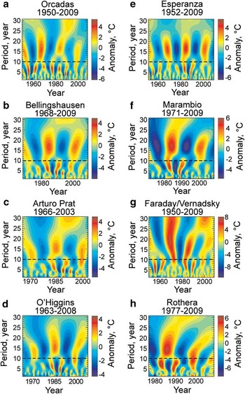
To present the oscillatory behaviour of the winter temperature in the AP region we first review the wavelet spectra of the individual station records. Figure 3 shows the wavelet transform of the eight time series. A clear separation between the oscillations with the periods shorter and longer than ten years marked by the dashed line can be seen from Fig. 3a–h.
Wavelet transform of the temperature time series for the eight stations of the Antarctic Peninsula region. a. Orcadas, b. Bellingshausen, c. Arturo Prat, d. O'Higgins, e. Esperanza, f. Marambio, g. Faraday/Vernadsky, and h. Rothera. Dashed lines at the 10 year period are drawn to show a separation of the oscillations with shorter and longer periods.

The temperature variability with the periods of three to eight years in Antarctica is associated with the main climatic modes of the Southern Hemisphere: SAM (Marshall Reference Marshall2007, Fogt et al. Reference Fogt, Perlwitz, Monaghan, Bromwich, Jones and Marshall2009) and Antarctic Circumpolar Wave (ACW; Connolley Reference Connolley2002, White et al. Reference White, Gloersen and Simmonds2004) affected by El Niño–Southern Oscillation (ENSO) through teleconnection (Turner Reference Turner2004). These temperature oscillations in Fig. 3 are enhanced during the 1950s (Orcadas, Esperanza & Faraday/Vernadsky; Fig. 3a, e & g, respectively) and during the 1980s.
Variability with periods longer than ten years (hereafter referred to as the decadal oscillation) appear more regularly over the observation interval. The wavelets for Bellingshausen, Esperanza & Marambio (Fig. 3b, e & f, respectively) show relatively steady decadal oscillations in comparison with those for other stations. The decadal variability is also discussed in the analysis of climatic modes, however, it is less studied in the station temperature records. The temperature trend calculated with overlapping time intervals (Vaughan et al. Reference Vaughan, Marshall, Connolley, Parkinson, Mulvaney, Hodgson, King, Pudsey and Turner2003, Turner et al. Reference Turner, Colwell, Marshall, Lachlan-Cope, Carleton, Jones, Lagun, Reid and Iagovkina2005) demonstrates decadal variability in the annual mean temperatures at the AP stations. Sansom (Reference Sansom1989) suggested an oscillatory trend in the winter temperature at Faraday with a period of around 16 years. Wavelet transform for Faraday/Vernadsky in Fig. 3g demonstrates probable correspondence with this result by the intense temperature oscillations with similar periodicity localized between the late 1960s and around 1990.
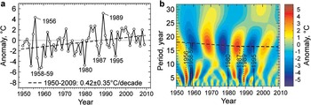
One can see the close coincidence in the timing of the decadal oscillation cycles among the eight stations (Fig. 3). For example, the two decadal maxima that appeared in the mid-1980s and around 2000 are observed in all time series. As a result, the averaged time series presented in Fig. 4a demonstrates the steady decadal cycles in the winter temperature change as seen from the wavelet spectrum in Fig. 4b. A separation between the two ranges of the temperature oscillation noted from Fig. 3 becomes even more evident from Fig. 4b. The decadal oscillation is relatively regular over the 1950–2009 period and shows maximum temperature deviations between around 1960 and 2000. Their mean period value decreased from c. 18 to 16 years in the first three decades (1950–80) as marked by horizontal dashed line in Fig. 4b. Note that the maximum temperature deviations are of comparable magnitude in both period ranges: around ± 6°C and ± 5°C for the three to eight year periods and for the decadal oscillation, respectively (Fig. 4b).
a. Time series of the temperature anomalies averaged over the eight stations in the Antarctic Peninsula region. Dashed line marks the linear temperature trend for the 1950–2009 period. b. Wavelet transform applied to the averaged anomaly time series in a. Horizontal dashed line at the maximum temperature deviations of the decadal oscillation marks their mean period.

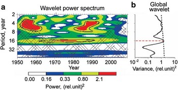
To present the Morlet wavelet power spectrum, we have used an independent analysis tool developed by Department of Atmospheric and Oceanic Sciences at the University of Colorado at Boulder (USA) which is available online from the NCEP-NCAR reanalysis web site, http://ion.researchsystems.com/IONScript/wavelet/. Outside the cone of influence (cross-hatched area), the decadal oscillation (power maximum at c. 16 years) is significant at the 10% level (black contour in the central part of Fig. 5a) during the 1970s and the early 1980s. The two spectral components in the global wavelet reach the 10% significance level and the maximum spectral power is at the 16 year period (Fig. 5b).
a. The wavelet power spectrum for the averaged time series shown in Fig. 4a, but standardized and detrended. The coloured contour levels are chosen so that 75%, 50%, 25%, and 5% of the wavelet power is above each level, respectively. The cross-hatched region is the cone of influence, where zero padding has reduced the variance. Black contour is the 10% significance level, using zero padding and a red noise (autoregressive lag-1) background spectrum. b. The global wavelet power spectrum (black line). The black dashed line is the significance for the global wavelet spectrum, assuming the same significance level and background spectrum as in a. The red dashed line marks the spectral power peak at the 16 year period. The plot was created using the analysis tool available at http://paos.colorado.edu/research/wavelets.

As noted above, oscillations with three to eight year periods are strongest during the 1950s and 1980s (Figs 4b & 5a). The second time interval corresponds to the ACW development with similar periodicity (Connolley Reference Connolley2002, White et al. Reference White, Gloersen and Simmonds2004). It could be assumed that the ACW-like event occurred also during the first time interval, in the 1950s. The data sources used in the ACW analysis are based mainly on the satellite observations which are absent before the 1970s (Connolley Reference Connolley2002, White et al. Reference White, Gloersen and Simmonds2004). There is a deficiency of earlier ground-based data in the West Antarctic thus preventing unambiguous detection of earlier ACW occurrences. The results of the wavelet analysis (Figs 4b & 5a) could be evidence of ACW-like oscillations with the maximum temperature deviations at the AP region longitudes during the 1950s.
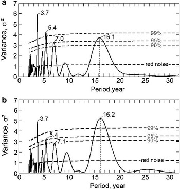
Note that a relationship between the spectral powers of the two spectral maxima in Fig. 5 could be influenced by outliers in the time series. This is illustrated by the Fourier power spectra in Fig. 6. The largest spectral power is at the 3.7 year period. If the outliers are removed, the power peak at c. 16 years becomes more than two times stronger than the peaks at the shorter periods (not shown). We show the spectrum change if the outliers are reduced to the 1σ level (Fig. 6b). The spectral power redistribution is clearly seen: the spectral peak at the 16 year period increases (both in power and statistical significance) relative to the spectral peaks at the shorter period. It could be evidence that, in the spectral estimates above, the outliers suppress the spectral power of the decadal oscillation to some degree.
Fast Fourier transform of the averaged time series shown in Fig. 4a but standardized and detrended. a. The solid curve is the normalized spectral power for the time series with the outliers. b. The solid curve is the normalized spectral power as in a., but the outliers are reduced to the 1σ level. The confidence intervals (90%, 95% and 99%, the three upper dashed curves) were calculated using the red noise background spectrum with the lag-1 autocorrelation (lower dashed curve).

The spectrum in Fig. 6a exhibits statistically significant periods close to those observed in the ACW variability (3.7, 7.1 and 17 years; White et al. Reference White, Gloersen and Simmonds2004). However, similar periodicity is also observed in the variability of the ENSO and SAM indices (Turner Reference Turner2004, Fogt et al. Reference Fogt, Perlwitz, Monaghan, Bromwich, Jones and Marshall2009). In the next subsection, we attempt to identify some of the largest winter temperature deviations with the strongest ENSO events.
Different estimates described above are probably consistent in the significance of the decadal component of the winter temperature oscillations in the AP region. Besides, as could be concluded from the wavelet and Fourier power spectra (Figs 4–6), the temperature oscillations with the periods of three to eight years and with the 16 year period probably have similar spectral power and statistical significance. This is evidence for nearly equal importance of the two spectral components for the winter temperature changes in the AP region.
Temperature extremes
The relationship between the amplitudes and phases of the temperature oscillations in the two period ranges (Fig. 4b) can be possibly related to the strength of the winter temperature extremes in the AP region. For example, one can consider the warm winters of 1956 and 1989 and the cold winters 1958–59, 1980, 1987 and 1995 (as labelled in Fig. 4). For these years, the regional scale temperature extremes coincide with those noted earlier in the winter temperatures at the individual AP stations (Schwerdtfeger Reference Schwerdtfeger1975, Marshall & King Reference Marshall and King1998, Ferron et al. Reference Ferron, Simões, Aquino and Setzer2004). Relative to the mean warming tendency (dashed line in Fig. 4a) the averaged temperature anomalies are higher than 5°C and lower than -3°C, for the warm and cold winters, respectively (with a standard deviation of the detrended time series of 2.1°C, t-parameter is 1.4–2.7). The coldest winters in Fig. 4a (1958–59, 1980 and 1995) are observed when the shorter period minima are temporally close to the decadal oscillation minima (the years of the coldest winter are marked by the solid vertical lines in Fig. 4b). This phase coincidence probably favoured the stronger temperature decrease. Opposing phases in 1987 (maximum in the decadal cycle and strong minimum in the shorter period range marked by dashed vertical line in Fig. 4b) may have weakened the temperature decrease for this winter (-3°C, Fig. 4a).
Figure 4b also demonstrates that the decadal oscillation does not contribute to the strong increase of the winter temperatures in 1956 and 1989 (Fig. 4a) because they have nearly zero amplitude these winters (dotted vertical lines in Fig. 4b). Hence, the temperature oscillations in a range of shorter periods seem to be responsible for the two warmest winters in the AP region during the last six decades. These winters could be associated with the cold ENSO events (La Niña) observed in the tropical Pacific in 1956 and 1989 (Trenberth & Stepaniak Reference Trenberth and Stepaniak2001, Turner Reference Turner2004).
A coupling between the cold (warm) ENSO events in the tropics and the warm (cold) winters in the AP region exists due to teleconnection via the stationary Rossby wave train (Turner Reference Turner2004). However, the teleconnection is not stable on long timescales and the correspondence between warm (cold) ENSO events and cold (warm) AP winters is not perfect (Marshall & King Reference Marshall and King1998, Turner Reference Turner2004). Nevertheless, as possible manifestations of the ENSO cycles, the two outliers of 1956 and 1989 (Fig. 4a) provide considerable contributions to the spectral power of the temperature oscillations with the period of three to eight years (Fig. 6).
The cold ENSO events during 1971–76 (Trenberth & Stepaniak Reference Trenberth and Stepaniak2001, Turner Reference Turner2004) did not have the expected responses in the winter temperature increase in the AP region. On the contrary, negative anomalies were observed these winters (Fig. 4a). If the warm ENSO events (El Niño) could be possibly related to the cold AP winters in 1958 and 1987, then the strongest El Niño in 1983 and 1998 had no similar effects since the positive temperature anomalies were observed in the AP region (Fig. 4a). Besides, there were no warm ENSO events to be associated with the cold winters 1980 and 1995. Generally, this agrees with the conclusions from the previous studies, that the high latitude atmosphere circulation can sometimes prevent the teleconnection effects in the AP temperature variability (Marshall & King Reference Marshall and King1998, Turner Reference Turner2004).
Decadal trends
The winter warming in the AP region estimated by the linear trend of the averaged temperature anomalies for the 1950–2009 period is 0.42 ± 0.35°C per decade which is significant at the 5% level (dashed line in Fig. 4a). In the detrended time series, the three outliers exceed the 2σ level (the anomalies of 1956, 1980 and 1989). After their removal via replacement with the means of the two neighbouring year anomalies, the trend value does not change noticeably (0.47 ± 0.26°C per decade) but increases in statistical significance (< 1%).
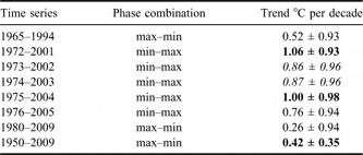
The results in Figs 4–6 suggest that this mean tendency occurs in the background and independently of the temperature oscillations associated with the shorter (three to eight year) and longer (c. 16 year) periods. Because the former are weak during several decades (Figs 4b & 5) the latter can have a greater influence on temperature changes. Table III illustrates the possible effects of the decadal oscillation cycles (Fig. 4b) in the decadal trends. The 30 year time intervals (see Table III) are chosen for comparison. They are shifted along the time axis by around a half period of the 16 year oscillation. As a result, the three alternating combinations of the decadal maxima and minima at the ends of these time intervals are presented in Table III.
Changes in decadal temperature trends in the Antarctic Peninsula region. The opposite phases of the decadal oscillation cycles (Fig. 4b) at the ends of the 30 year intervals are presented. The 95% confidence intervals with a lag-1 autocorrelation are shown and the trend values significant at the 5% (10%) level are in bold (italic).
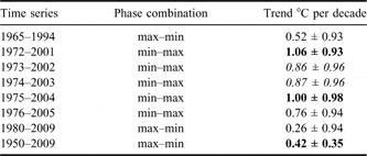
It is clear that the years with persistently higher (lower) temperatures at the start of these partial time series favour a decreased (increased) trend line inclination. The inverse relationship should take place at the end of the time series. As seen from Table III, the ‘max–min’ phase combination at the ends of the 30 year intervals (1965–94 and 1980–2009) results in relatively low and statistically insignificant trends. As expected, the inverse phase combination (min–max in 1972–2001, 1973–2002, 1974–2003 and 1975–2004) gives higher decadal trends at 0.9°C per decade to 1.1°C per decade, significant at the 5–10% levels. It should be emphasized that the outliers (see Fig. 4) do not contribute significantly to the edge effect that is analysed.
Winter climatic changes in the AP region show strong spatial differentiation with the most evident warming in the western AP (Vaughan et al. Reference Vaughan, Marshall, Connolley, Parkinson, Mulvaney, Hodgson, King, Pudsey and Turner2003, Turner et al. Reference Turner, Colwell, Marshall, Lachlan-Cope, Carleton, Jones, Lagun, Reid and Iagovkina2005). The high decadal trend value of c. 1°C per decade is usually referred to the local observations at Faraday/Vernadsky (Vaughan et al. Reference Vaughan, Marshall, Connolley, Parkinson, Mulvaney, Hodgson, King, Pudsey and Turner2003, Turner et al. Reference Turner, Colwell, Marshall, Lachlan-Cope, Carleton, Jones, Lagun, Reid and Iagovkina2005, Roscoe et al. Reference Roscoe, Marshall and King2006). The results shown in Table III are evidence that 30 year time intervals existed when the same warming rate was observed over the whole AP region. This rapid regional winter warming is associated with the decadal oscillation (Fig. 4b), namely, with the largest negative temperature deviation during the 1970s (-4°C to -5°C) which is combined with the moderate positive deviation in the early 2000s (2–3°C).
Decadal temperature extremes at the ends of the whole period 1950–2009 (2°C and -2°C, respectively; Fig. 4b) probably favour a relatively lower trend estimate than could be derived in the absence of the decadal temperature modulation. As the 16 year periodicity appears rather stable over the greater part of the analysed period (Figs 4b & 5a), it could be concluded that the winter warming estimates in the AP region could be dependent on the time series length and on the decadal oscillation amplitude and phase at the time series ends. This dependence could be a possible factor influencing the decadal variability in the annual mean temperature trends noted in (Vaughan et al. Reference Vaughan, Marshall, Connolley, Parkinson, Mulvaney, Hodgson, King, Pudsey and Turner2003, Turner et al. Reference Turner, Colwell, Marshall, Lachlan-Cope, Carleton, Jones, Lagun, Reid and Iagovkina2005).
Discussion
In this study, we analysed the variability of the winter temperatures in the Antarctic Peninsula region using the Met READER data for the eight stations over the 1950–2009 period. Fourier and wavelet analysis of the averaged anomaly time series indicated the occurrence of: i) a decadal oscillation with around a 16 year period and a maximum spectral power during the 1970s, and ii) enhanced oscillations with the periods of three to eight years within the two time intervals covering mainly the 1950s and the 1980s. Both spectral components are of around the same spectral power and statistical significance (Figs 4b, 5 & 6).
Owing to different distributions of the spectral power in time, the two spectral components add variable relative contributions to winter temperature changes in the region. This was illustrated by the relationships between their amplitudes and phases and the occurrences of the coldest/warmest winters (Fig. 4), as well as by the decadal trend estimates that depended on the timing of the decadal oscillation cycles (Table III).
The coupled processes in the atmosphere, ocean and sea ice are among possible candidate mechanisms influencing the temperature variability in the AP region that can be considered (Vaughan et al. Reference Vaughan, Marshall, Connolley, Parkinson, Mulvaney, Hodgson, King, Pudsey and Turner2003, Yuan & Li Reference Yuan and Li2008, Turner & Overland Reference Turner and Overland2009). The Antarctic stations in the AP region are located close to the sea ice boundary and a small reduction in sea ice can have a large impact on the air temperatures, so that the higher (lower) temperatures are probably associated with lower (higher) sea ice concentrations (King Reference King1994, Ferron et al. Reference Ferron, Simões, Aquino and Setzer2004, Turner et al. Reference Turner, Colwell, Marshall, Lachlan-Cope, Carleton, Jones, Lagun, Reid and Iagovkina2005). In the satellite derived winter temperatures over the 1982–2000 period, a high spatial coherence exists not only along the western Antarctic Peninsula (r > 0.75), but also in the large region extending northwards into the Drake Passage and eastwards into the Weddell and Scotia seas (r > 0.5, King & Comiso Reference King and Comiso2003). Our estimates of the correlation between the station records over the last three to six decades (Table II) show similar r-values and their spatial distribution. Figure 7 illustrates the coupled patterns in the variability of air temperatures and sea ice concentration which could be a possible factor of the spatial coherence in the station records of the AP region.
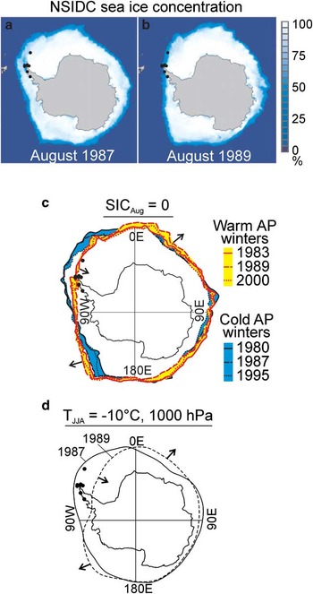
Monthly mean sea ice concentration in August a. 1987, and b. 1989 with total sea ice areas of 13.9 million km2 in both years. c. Range of sea ice-edge variability in August of cold (1980, 1987 and 1995; blue fill) and warm (1983, 1989 and 2000; yellow fill) Antarctic Peninsula winters by the NSIDC sea ice concentration at zero level. d. Contours of air temperature -10°C at the 1000 hPa pressure level in winters (June–August) 1987 (solid line) and 1989 (dashed line) by the NCEP R-2 data. Arrows in c. and d. show displacement of the warm-winter contours relative to the cold-winter contours. Black dots mark the station locations.

The monthly images of the sea ice concentration (SIC) were obtained from the NSIDC data (Cavalieri et al. Reference Cavalieri, Parkinson, Gloersen and Zwally1996). The upper two plots (Fig. 7a & b) show the Antarctic sea ice distributions in August (i.e. in the late winter, when the ice cover usually approaches its maximum area) 1987 and 1989, the years of the extremely cold and warm winters, respectively, in the AP regions (Fig. 4a).
It is seen from Fig. 7a & b that the SIC variability along the east coast of Antarctica is not as large as in West Antarctica and the stations in the AP region (black dots) are indeed similar with regard to the sea ice advance/retreat. Black (red) contours of zero SIC in Fig. 7c demonstrate that the sea ice-edge in the quadrant 0°E–90°W typically takes the most northern (southern) location in the cold (warm) winters 1980, 1987 and 1995 (1983, 1989 and 2000). Opposite displacement is seen in the quadrant 90–180°W (as marked by arrows; also compare the positions of the areas filled by blue and yellow in Fig. 7c for the cold and warm winters, respectively). Note an equality of the total sea ice area from the NSIDC data for August 1987 and 1989 (13.9 million km2; Fig. 7a & b). Hence, in the large-scale interannual SIC variations in West Antarctic, a spatial redistribution rather than significant change in the total sea ice area could be possible (Fig. 7c).
These changes in the sea ice-edge position are associated with the analogous redistributions in the temperature field as seen from the -10°C contours in Fig. 7d. The seasonal mean temperatures (June–August) for the 1000 hPa pressure level were obtained from the NCEP R-2 data (Kanamitsu et al. Reference Kanamitsu, Ebisuzaki, Woollen, Yang, Hnilo, Fiorino and Potter2002). Spatially, the shift of temperature contours in the quadrant 0°E–90°W is larger than in the sea ice-edge in Fig. 7a–c, in agreement with many previous studies (King Reference King1994, Ferron et al. Reference Ferron, Simões, Aquino and Setzer2004, Turner et al. Reference Turner, Colwell, Marshall, Lachlan-Cope, Carleton, Jones, Lagun, Reid and Iagovkina2005). Due to such the poleward (equatorward) contour displacements in the warm (cold) winters (Fig. 7d), the common component in the temperature variability at the eight stations considered can appear. Regardless of the source of these large-scale displacements, the spatial coherence in temperature variability could exist on interannual to decadal timescales.
The sea ice-air temperature variability in Fig. 7 demonstrates the zonally asymmetric pattern that may be related to quasi-stationary planetary waves (Hobbs & Raphael Reference Hobbs and Raphael2009 and citations therein). This pattern could be formed under the influence of ENSO, SAM and ACW, which are coupled modes of the climate variability (e.g. Ciasto & Thompson Reference Ciasto and Thompson2008, Yuan & Li Reference Yuan and Li2008). The results above are also evidence of ENSO and ACW influence. The individual events have been identified comparing the wavelet spectrum and winter temperature extremes (Fig. 4) with the strongest ENSO. Antarctic Circumpolar Wave-like oscillations are observed in the wavelet spectra of the averaged time series (Figs 4b & 5a). By our estimate, the correlation between the averaged time series (Fig. 4a) and the Marshall SAM index is r = 0.35 ± 0.24 significant at the 1% level. Significant positive correlations between the SAM and winter temperatures (r = c. 0.5) were noted by Marshall (Reference Marshall2007) for Orcadas and Esperanza (see Fig. 2 in Marshall Reference Marshall2007). This suggests a contribution of the SAM to winter temperature variations in the AP region, although it is not a predominant factor.
The effects of ENSO, SAM and ACW in Antarctica are observed at periods of three to eight years (Turner Reference Turner2004, White et al. Reference White, Gloersen and Simmonds2004, Fogt et al. Reference Fogt, Perlwitz, Monaghan, Bromwich, Jones and Marshall2009). It has been shown earlier that the ENSO teleconnection is irregular in the AP region (Marshall & King Reference Marshall and King1998, Turner Reference Turner2004) and the ACW-like oscillation in the West Antarctica is not continuously observed (Connolley Reference Connolley2002, White et al. Reference White, Gloersen and Simmonds2004). These could be possible causes of the spectral energy distribution in the regional temperature variability with three to eight year periods (Figs 4–6).
The observed decadal oscillation with around a 16 year period appears more persistent (Figs 4b & 5a), however, in the scope of this work, it has not been clearly attributed to any mode of the climate variability and needs further study. A 17 year periodicity was also noted in the ACW oscillation (White et al. Reference White, Gloersen and Simmonds2004) but the ACW did not appear during the decade of the maximum signal in the decadal oscillation (1970s, Fig. 5a). In the Southern Ocean, the Antarctic Circumpolar Current could also be a source of the low frequency periodic oscillation (e.g. Hogg & Blundell Reference Hogg and Blundell2006). The most intense and steady decadal oscillation is seen from the wavelets for BEL, ESP and MAR (Fig. 3b, e & f, respectively), i.e. for the stations at the northern part of the Antarctic Peninsula. This indicates that the regional effects of the oceanic/atmospheric circulation variability could be possible. On the other hand, the 15–18 year interdecadal periodicity was noted in the global temperature variability (Mann & Park Reference Mann and Park1999, figs 18 & 22).
Conclusions
The objective of this study was to examine long-term winter temperature changes in the Antarctic Peninsula region. We analysed average temperature anomalies for eight temperature recording stations over the six decades (1950–2009). The results of Fourier and wavelet analyses suggested the occurrence of two significant spectral components: oscillations with periods of three to eight years and a decadal oscillation with a period of around 16 years. Both spectral components have similar spectral power and statistical significance and could be of comparable importance for winter temperature changes in the AP region.
The three to eight year oscillations are most probably tied to ENSO and ACW events. It has been shown that there were the four temperature extremes in the averaged time series which could be related to the ENSO events. On the other hand, some of the strongest ENSO events did not affect regional winter temperatures. Oscillations with periods of three to eight years with the maximum spectral power in the 1980s are probably associated with ACW development. It has been hypothesized that similarly intensified oscillations in the 1950s could also be related to ACW influences and this has not been described previously. As the ENSO and ACW signals appear within the same oscillation sequences during the 1950s and the 1980s, this could be a manifestation of an ENSO-ACW coupling (e.g. Connolley Reference Connolley2002, Yuan & Li Reference Yuan and Li2008).
The newly discovered decadal oscillation with a 16 year period has not been clearly attributed in this analysis to any particular mode of climate variability and it deserves further study. It has been shown that the relationships between the amplitudes and phases of the two spectral components can affect the winter temperature extremes in the AP region. Besides, the decadal trend estimates show that the decadal oscillation can modulate the regional warming to some degree: the 30 year time intervals existed when the decadal trends reached c. 1°C per decade, i.e. the warming rate which is usually referred to the local observations at Faraday/Vernadsky.
Acknowledgements
We acknowledge the SCAR READER database for free access to the monthly data of the Antarctic station temperatures. We thank the Department of Atmospheric and Oceanic Sciences of the University of Colorado at Boulder, USA, for the accessibility of the wavelet analysis tool at http://paos.colorado.edu/research/wavelets. We thank National Snow and Ice Data Center (NSIDC), USA, for the sea ice concentrations from Nimbus-7 SMMR and DMSP SSM/I Passive Microwave Data available at http://nsidc.org/data/nsidc-0051.html. NCEP_Reanalysis 2 data provided by the NOAA/OAR/ESRL PSD, Boulder, Colorado, USA, from their web site at http://www.esrl.noaa.gov/psd. The research was supported by the project of Taras Shevchenko National University of Kyiv, No. 11BF051-01. The authors thank two anonymous referees for useful comments and remarks that assisted in improving the manuscript.