1. INTRODUCTION
This paper is concerned with inference in the standard linear instrumental variable (IV) regression model with possibly weak IVs. We start by giving a brief account of recent developments in the literature on weak IVs to explain the contribution of this paper to the literature. It has been documented in the weak IV literature that standard methods, such as two-stage least squares–based tests and confidence intervals (CIs), perform poorly when IVs are weak, especially when endogeneity is moderate to strong. Specifically, such tests have size well in excess of their nominal level, and corresponding CIs have size well below their nominal level. See the review papers of Stock, Wright, and Yogo (2002), Dufour (2003), and Andrews and Stock (in press).
The well-known Anderson and Rubin (1949) (AR) test does not exhibit size distortions due to weak IVs. Hence, Staiger and Stock (1997) and Dufour (1997) propose basing inference on the AR test. AR-based CIs can be constructed by inverting AR tests. The AR test has good power properties when the model is just identified; see Moreira (2001) and Andrews, Moreira, and Stock (2006a) for some optimality properties for the case of Gaussian errors. However, the AR test sacrifices power when the model is overidentified. This leads to excessively long AR-based CIs.
In consequence, considerable effort has been expended recently to develop new tests that circumvent this problem. Such tests are of interest in their own right and because they can be used to construct CIs by inversion. Kleibergen (2002) and Moreira (2001) introduce a Lagrange multiplier (LM) test whose size is robust to weak IVs and whose power exceeds that of the AR test in many cases when the model is overidentified. However, this test has somewhat quirky power properties. For example, its power function can be nonmonotonic; see Andrews et al. (2006a, 2006b).
Subsequently, Moreira (2003) showed that any test can be made robust to weak IVs asymptotically by using a conditional critical value function that conditions on a statistic that is complete and sufficient under the null hypothesis. Using this method, he introduced the conditional likelihood ratio (CLR) test. Andrews et al. (2006a) investigate the power properties of the CLR test in the case of a single right-hand-side endogenous variable and show that its power is essentially on the asymptotic power envelope for two-sided invariant similar tests under the assumption of Gaussian errors. This is true under both the “weak IV asymptotics” introduced in Staiger and Stock (1997), in which the coefficient on the IVs in the first-stage regression shrinks to zero as the sample size goes to infinity, and under the standard “strong IV asymptotics.” Andrews and Stock (in press) show that these optimality properties extend to the “many weak IV asymptotic scenario,” in which the number of IVs increases with the sample size. Hence, the CLR test has the desirable features of having size that is robust to weak IVs and near-optimal power properties with Gaussian errors.1
We note that the CLR test reduces to the AR test when the model is just-identified, and so the optimality properties mentioned in the text are consistent with those mentioned previously for the AR test.
In this paper, we aim to further improve the power properties of weak IV tests by constructing a test that has the same asymptotic behavior as the CLR test with Gaussian errors but improved power with non-Gaussian errors. To do this, we construct a rank analogue of the CLR test, denoted RCLR. We also construct a rank analogue of the LM test of Kleibergen (2002) and Moreira (2001), denoted RLM. As is well known from location and regression models, rank estimators and tests have more robust efficiency properties than least squares–based procedures; see Hettmansperger (1984). For example, Chernoff and Savage (1958) have shown that the asymptotic relative efficiency (ARE) of the normal scores rank test to the analogous least-squares t-test is greater than or equal to one for all symmetric error distributions with equality at the Gaussian. This holds in both location and regression models, and it also holds for estimators. This suggests that for the linear IV model rank-based tests whose size is robust to weak IVs may exhibit similarly desirable power properties under nonnormality.
Andrews and Marmer (in press) develop a rank analogue of the AR test, denoted RAR. This test has exact finite-sample size under Gaussian and non-Gaussian errors under certain circumstances. Its asymptotic power properties improve on those of the AR test and are excellent for just-identified models. However, as with the nonrank AR test, the RAR test sacrifices power in overidentified models. The RCLR and RLM tests developed here substantially improve the power properties of the RAR test in overidentified models.
We now summarize the results of the paper. The model considered is a linear IV regression model with a single structural equation with m right-hand-side endogenous variables and p exogenous variables coupled with m reduced-form equations for the right-hand-side endogenous variables. The null hypothesis is H0 : β = β0, where β is the m-dimensional coefficient on the m right-hand-side endogenous variables. The alternative hypothesis is H1 : β ≠ β0.
First, we introduce rank analogues of the CLR and LM tests. This is more difficult than for the AR test because the LR and LM statistics are more complicated functions of the data than is the AR statistic. A hybrid rank/linear test statistic is required to obtain power properties of RCLR and RLM tests that are analogous to those of the CLR and LM tests under Gaussianity and superior for other distributions.
Second, we obtain the weak IV asymptotic distributions of the rank statistics under the null and fixed alternatives. These results are used to show that under Gaussian errors the normal scores (NS) RCLR and RLM tests have the same null and alternative asymptotic behavior as the nonrank versions of these tests. The same is true for the Wilcoxon scores (WS) rank and nonrank CLR and LM tests under uniform errors. Furthermore, these asymptotic distributions allow one to compare the weak IV asymptotic power of the rank to nonrank tests under different error distributions. It is shown that the same AREs for the rank versus nonrank LM and AR tests arise in the weak IV context as in the location and regression models. Hence, the Chernoff–Savage result also applies to these tests. That is, the NS-RLM test (weakly) dominates the LM test in terms of power for all symmetric error distributions, and the same is true for the NS-RAR test versus the AR test.
For the rank versus nonrank CLR tests, the weak IV asymptotic power comparison is more complicated. However, numerical calculation of the asymptotic powers of these tests shows the same pattern that is typical for rank versus nonrank procedures in other contexts. In particular, the NS-RCLR test has noticeably higher asymptotic power for thin-tailed (uniform) and thick-tailed (t3 and difference of independent log normals (DLN)) errors than the nonrank CLR test and equal asymptotic power for Gaussian errors. The WS-RCLR test has asymptotic power that is close to that of the CLR test for Gaussian and uniform errors and substantially higher power for t3 and DLN errors.
Third, we establish the strong IV asymptotic distributions of the rank statistics under the null and local alternatives. These results show that the RCLR and RLM tests are asymptotically equivalent under strong IV asymptotics. This is also true of the nonrank versions of these tests. The results also show that the ARE of the rank to the nonrank versions of these tests under strong IV asymptotics is the same as the standard ARE that arises in location and regression models for tests and estimators. Hence, the Chernoff–Savage result applies under strong IV asymptotics to both the NS-RCLR test and the NS-RLM test. In consequence, the NS-RCLR test (weakly) dominates the CLR test in terms of power for symmetric errors under strong IV asymptotics.
The proofs of the weak and strong IV asymptotic results make use of results and arguments given in Hájek and Sidák (1967) and Koul (1969, 1970).
Fourth, we carry out finite-sample size and power comparisons of the WS-RCLR, NS-RCLR, CLR, LM, and AR tests. For brevity, we do not report results for the RLM and RAR tests, because they are found to be inferior (both asymptotically and in finite-sample experiments) to those of the RCLR tests. We compare the tests for a variety of scenarios that differ according to the degree of endogeneity, strength of the IVs, number of IVs, and size of the sample. For each scenario we consider Gaussian, uniform, t1, t2, t3, and DLN errors. The two RCLR tests perform noticeably better in terms of size than the nonrank CLR, LM, and AR tests. The finite-sample power comparisons reflect the asymptotic power comparisons discussed previously fairly closely. Specifically, the NS-RCLR test has similar power to the CLR test for Gaussian errors and higher power for non-Gaussian errors. The WS-RCLR test does not perform as well as the NS-RCLR test with uniform errors, but it performs better with thick-tailed errors.
Based on the asymptotic and finite-sample results, we recommend the NS-RCLR test over the WS-RCLR, CLR, LM, and AR tests. The WS-RCLR test also has good overall properties, but we prefer the NS-RCLR test because of its excellent power performance for both thin-tailed and thick-tailed errors.
The main drawback of the RCLR tests is that they are not robust to heteroskedasticity of the errors. That is, their size may be distorted by heteroskedasticity. This is also true of the CLR test. However, it is possible to robustify the CLR test to heteroskedasticity; see Andrews, Moreira, and Stock (2004) and Kleibergen (2005). It is not possible to robustify the RCLR tests to heteroskedasticity. Hence, there is a trade-off between power for non-Gaussian errors and robustness to heteroskedasticity for these tests. If heteroskedasticity is a possible problem, then the robustified CLR test is preferred to the NS-RCLR and WS-RCLR tests. If not, then the rank tests are preferred.
There is a vast literature on rank procedures in statistics; e.g., see Hájek and Sidák (1967), Hettmansperger (1984), Puri and Sen (1985), and Hájek, Sidák, and Sen (1999). Rank procedures have been used in both cross-section and time series econometrics. For a review, see Koenker (1996). Some more recent econometric references include Hasan and Koenker (1997), Cavanagh and Sherman (1998), Abrevaya (1999), Chen (2000, 2002), and Thompson (2004).
The remainder of this paper is organized as follows. Section 2 defines the model. Section 3 introduces the rank analogues of the CLR, LM, and AR tests. Sections 4 and 5 provide asymptotic results for these tests under weak IV and strong IV asymptotics, respectively. These sections also give asymptotic power comparisons of rank and nonrank tests. Section 6 provides finite-sample size and power comparisons of rank and nonrank tests. An Appendix contains proofs of the results.
All limits are taken as n → ∞, and vec(·) is the column by column vec operator.
2. MODEL
We consider the following model, which consists of a single structural equation and m reduced-form equations:

where y1i ∈ R, y2i ∈ Rm, Xi ∈ Rp, and

are observed variables; ui ∈ R and v2i ∈ Rm are unobserved errors; and β ∈ Rm, Π ∈ Rk×m, γ1 ∈ Rp, and ξ1 ∈ Rp×m are unknown parameters.
Our interest is in testing the hypotheses

Let

and X denote the n × k IV and n × p regressor matrices whose ith rows are

and Xi′, respectively. We transform the IV matrix

so that the transformed IV matrix, Z, and the regressor matrix, X, are orthogonal:

where Zi is the ith row of Z written as a column and

. By construction, Z′X = 0.
Substituting the reduced-form equations for y2i into the structural equation for y1i yields m + 1 reduced-form equations:

and γ = γ1 + ξβ. The m + 1 reduced-form equations also can be written as

Let Y and Y2 denote the n × (m + 1) and n × m matrices whose ith rows are yi′ and y2i′, respectively.
We make the following basic assumptions about the model. (Additional assumptions are given subsequently.)
Assumption 1.
(a) {(ui,v2i) : i ≥ 1} are independent and identically distributed (i.i.d.) random variables with mean zero.
(b) v2i has nonsingular variance matrix Ω22 ∈ Rm×m.
Assumption 2.
(a)

are fixed (i.e., nonrandom).
(b) The first element of Xi is 1 for all i.
(c)

.
(d)

.
The combination of Assumptions 1 and 2(a) implies that the distribution of the errors {(ui,v2i) : i ≥ 1} does not depend on the IVs or regressors. In place of Assumption 2(a), one could treat the IVs and regressors as random. In this case, the IVs and regressors would be assumed to be independent of the errors. As is, Assumption 2(a) is consistent with random IVs and regressors provided one conditions on these variables.
Assumption 2(b) requires that the structural and reduced-form equations include an intercept. Given that Z′X = 0, this implies that

. Assumptions 2(c) and 2(d) are standard assumptions concerning the behavior of IVs and regressors. They hold with probability one if

is a realization of an i.i.d. sequence with positive definite (pd) variance matrix and 2 + δ moments finite for some δ > 0; see Lemma 12 in the Appendix.
We now define the CLR test of Moreira (2003), the LM test of Kleibergen (2002) and Moreira (2001), and the AR test. The CLR test depends on an LR test statistic coupled with a “conditional” critical value defined subsequently. The LR, LM, and AR test statistics are based on the following statistics:2
The statistics Sn and Tn are denoted S and T, respectively, in Moreira (2003).

Note that

is an estimator of the variance matrix Ω = Evivi′, which needs to be well defined and pd for Sn and Tn to be well behaved asymptotically. After proper centering, the statistics Sn and Tn have a joint multivariate normal asymptotic distribution with zero covariance under weak IV asymptotics under the null and the alternative. Hence, Sn and Tn are asymptotically independent.
The LR, LM, and AR test statistics depend on (Sn,Tn) in the following way:

where λmin(C) denotes the minimum eigenvalue of the matrix C. When m = 1, LRn can be written as

see Moreira (2003) and Andrews and Stock (in press).3
The statistic LRn is the likelihood ratio statistic for the case of normal errors vi with known covariance matrix Ω and with

plugged in for Ω. One can also consider the likelihood ratio statistic for the case of normal errors and unknown covariance matrix; see Moreira (2003).
The CLR test with asymptotic level α rejects the null hypothesis when

where κLR,α(·,k,m) is a critical value function defined such that the CLR test has asymptotic null rejection rate α under weak IV asymptotics (under the preceding assumptions and Eui2 < ∞). See (3.10) for the definition of κLR,α(·,k,m).
The LM statistic has a chi-squared asymptotic null distribution with m degrees of freedom, denoted χm2, under weak and strong IVs (under the preceding assumptions and Eui2 < ∞). Hence, the critical value for the asymptotic level α LM test is the 1 − α quantile of a χm2 distribution.
The AR statistic times k has a chi-squared asymptotic null distribution under weak and strong IVs with k (≥ m) degrees of freedom (under the preceding assumptions and Eui2 < ∞). Under the assumption of normal errors {vi : i ≥ 1}, it has an exact Fk,n−k−p distribution. Thus, use of the 1 − α quantile of an Fk,n−k−p distribution as the critical value for the level α AR test is justified asymptotically for nonnormal errors and yields an exact test for normal errors.
3. RANK CLR, LM, AND AR TESTS
In this section, we introduce rank analogues, Snφ and Tnφ, of the statistics Sn and Tn, where φ is a score function defined subsequently. By design, Snφ and Tnφ are asymptotically independent. Given Snφ and Tnφ, we define rank statistics that are analogous to the CLR, LM, and AR statistics defined previously. We show that for normal scores, i.e., φ = φNS, and multivariate normal errors (ui,v2i), Snφ and Tnφ are asymptotically equivalent to Sn and Tn under weak IV and strong IV asymptotics under the null and the alternative. For nonnormal errors, the rank tests have power advantages.
The statistic Sn depends on the inner product of Z and a vector of null-restricted residuals from the structural equation (2.1):

where

is some estimator of γ1 and the second equality holds because Z′X = 0. The rank analogue of Sn that we consider depends on the inner product of Z with the vector of ranks of

.
Let

be some “null-restricted” estimator of γ1. For example, one could use the least squares (LS) null-restricted estimator:

Estimators other than the LS estimator could be considered, but the LS estimator is convenient because it is easy to compute. (The LS estimator satisfies the assumptions given subsequently provided the errors have finite variances.)
Let

be the rank of

in

. The ranks

are referred to as aligned ranks.
4If there are any ties in the ranks, then we determine a unique ranking by randomization. For example, if

for some i ≠ j and these observations are the [ell ]th largest in the sample, then

with probability 0.5,

with probability 0.5,

if

, and

if

. Ties only occur with positive probability if the distribution of

is not absolutely continuous. In consequence, in practice ties rarely occur.
The matrix programming languages GAUSS and Matlab have very fast built-in procedures for finding the ranks of a given vector. The GAUSS procedure is called rankindx.
Let φ : [0,1) → R be a nonstochastic score function. Different score functions φ lead to different rank statistics. Of primary interest are (a) the normal (or van der Waerden) score function and (b) the Wilcoxon score function:

where Φ−1(·) is the inverse standard normal distribution function (df). Define

For normal scores,

.
Let Rφ denote the n-vector whose ith element is

. The rank analogue of Sn is

The rank statistic Snφ replaces

in Sn by Rφcφ−1/2. We want the rank analogue of Tn to do the same and also to be asymptotically independent of Snφ. In consequence, to construct a rank analogue of Tn, it is helpful to rewrite Tn as follows:

(See (A.81) in the Appendix for a proof of (3.6).) As defined,

is an estimator of the asymptotic variance matrix, Ω*, of

. The definition of

is chosen to yield asymptotic independence of Sn and Tn.
The rank analogue of Tn is5
The definition of Tnφ uses the ranks Rφ of

but is linear in Y2 (or equivalently, in Y2 − PXY2 because Z′PX = 0). One might think that it is more natural to replace Y2 in the definition of Tnφ by the ranks of Y2 − PXY2. We do not do this for the following reason. For power purposes one wants the Y2 term in the definition of Tnφ to be (asymptotically) linear in its mean ZΠ. If one replaces Y2 by the ranks of Y2 − PXY2, then (asymptotic) linearity does not hold under strong IV asymptotics, defined in Section 5, because ZΠ is not an n−1/2 perturbation from the zero vector; see Lemma 6 in the Appendix. Hence, one does not obtain the desired power properties under strong IV asymptotics. Under weak IV asymptotics, defined in Section 4, (asymptotic) linearity holds because ZΠ = ZCn−1/2 for some matrix C and the latter is an n−1/2 perturbation from the zero vector. Hence, power problems with this alternative definition of Tnφ only arise under strong IV asymptotics.

Note that

is an estimator of the asymptotic variance matrix of

. The definition of

ensures that Snφ and Tnφ are asymptotically independent.
We define the rank LR, LM, and AR statistics to be

For m = 1, the RLRnφ statistic simplifies as in (2.8) with (Snφ,Tnφ) in place of (Sn,Tn).
Notice that when k = m (i.e., the structural equation is just identified), k·RARnφ = Snφ′Snφ = RLMnφ = RLRnφ.6
The second equality holds because Tnφ is a square invertible matrix when k = m. The last equality holds because [Sn : Tn]′[Sn : Tn] is positive semidefinite and singular, which implies that λmin([Sn : Tn]′[Sn : Tn]) = 0. Singularity holds because [Sn : Tn]′ is an (m + 1) × m matrix and [Sn : Tn]′[Sn : Tn] is (m + 1) × (m + 1) when k = m.
The rank CLR, LM, and AR tests use the same critical values as the nonrank versions of these tests. Hence, the rank LM and AR tests with asymptotic significance level α have critical values given by the 1 − α quantiles of the χm2 and Fk,n−k−p distributions, respectively.
The rank CLR test rejects the null hypothesis if

where κLR,α(·,k,m) is defined as follows. For t ∈ Rk×m, define κLR,α(t′t,k,m) via

for s ∈ Rk. Note that κLR,α(·,k,m) depends on k (the dimension of Zi) and m (the dimension of y2i). Andrews et al. (2006b) provides detailed tables of κLR,α(τ,k,m) for m = 1 and a variety of values of τ and k. Andrews, Moreira, and Stock (in press) provide a GAUSS program for computing p-values of the CLR test for m = 1 and arbitrary k. This program also can be used for the rank CLR test by replacing the Andrews et al. (2006a)

and

statistics by RLRnφ and Tnφ′Tnφ, respectively.
For m > 1, the critical value function κLR,α(·,k,m) can be simulated quite easily by simulating S0(r) ∼ iid N(0,Ik) for r = 1,…,Reps and taking κLR,α(t′t,k,m) to be the 1 − α sample quantile of {LR∞(S0(r),t) : r = 1,…,Reps}, where Reps is a large integer, such as 25,000.
4. WEAK IV ASYMPTOTIC RESULTS
4.1. Weak IV Asymptotic Distributions of Rank Statistics
In this section, we establish the weak IV asymptotic distributions of the RLRnφ, RLMnφ, and RARnφ test statistics under the null and fixed β alternatives.
We assume that the score function φ satisfies the following condition.
Assumption 3.
(a) φ : [0,1) → R is absolutely continuous and bounded with two derivatives that exist almost everywhere and are bounded.
(b) 0 < cφ < ∞ for cφ defined in (3.4).
Assumption 3 holds for Wilcoxon scores. Assumption 3(b) holds for normal scores, but Assumption 3(a) does not. However, normal scores that are smoothly truncated above and below near 0 and 1 satisfy Assumptions 3(a) and 3(b). Simulation results given subsequently for untruncated normal scores indicate that truncation is not necessary in practice.
Under weak IVs, the asymptotic variance matrix, Ωφg, of

is defined by

G is the df of ui + (β − β0)′v2i, and g is the density corresponding to G.7
Var(φ(Ugi)) = cφ because Ugi has a U[0,1] distribution.
Let I(f) denote Fisher's information of an absolutely continuous density f. That is, I(f) = ∫[f′(x)/f(x)]2f(x)dx.
The weak IV assumption is the first part of the following assumption.
Assumption 4W.
(a) Π = Cn−1/2 for some matrix C ∈ Rk×m.
(b) β does not depend on n.
(c) ui + (β − β0)′v2i has an absolutely continuous strictly increasing df G and an absolutely continuous and bounded density g that satisfies I(g) < ∞.
(d) (ui + (β − β0)′v2i,v2i) has an absolutely continuous bounded joint density with partial derivative with respect to its first argument that is bounded over both arguments.
(e) Ωφg is pd.
(f)

.
Assumption 4W(b) implies that the data-generating process satisfies the null hypothesis or a fixed β alternative. Assumptions 4W(c) and (d) require that (ui + (β − β0)′v2i,v2i) is absolutely continuous but otherwise are not very restrictive. Note that Assumptions 1–3 and 4W place no moment restrictions on ui.
Assumption 4W(f) requires the null-restricted estimator

to be well behaved. It is satisfied by the LS estimator under the preceding assumptions if Eui2 < ∞.
LEMMA 1. Under Assumptions 1, 2, 4W(a), and 4W(b) and Eui2 < ∞,

satisfies Assumption 4W(f).
We show that Snφ and Tnφ converge in distribution to independent random quantities S∞φ ∈ Rk and T∞φ ∈ Rk×m, respectively, that are defined as follows. Let DZ ∈ Rk×k be the probability limit of n−1Z′Z:

where D11 ∈ Rk×k, D12 ∈ Rk×p, and D22 ∈ Rp×p.
For a score function φ and a density f, define

and f′ denotes the derivative of f. For normal and Wilcoxon scores,

respectively, where φ and Φ denote the standard normal density and df and F′ = f.8
The expressions for ξ(φ,f) for normal and Wilcoxon scores are established by change of variables and integration by parts.
Let [Nφ : N2] be a k × (m + 1) multivariate normal matrix with

where g is the density of ui + (β − β0)′v2i; see Assumption 4W(c). Now, define

Under H0, S∞φ has mean zero, but T∞φ does not. It is shown subsequently that the covariance of S∞φ and T∞φ is zero and hence these normal random variates are independent (under H0 and H1).
The following result holds under the null hypothesis and fixed β (i.e., nonlocal) alternative hypotheses.
THEOREM 1. Under Assumptions 1–3 and 4W,
(i) (Snφ,Tnφ) →d (S∞φ,T∞φ), where S∞φ and T∞φ are independent,
(ii) RLRnφ →d LR∞φ := S∞φ′S∞φ − λmin([S∞φ : T∞φ]′[S∞φ : T∞φ]),
(iii) RLMnφ →d S∞φ′T∞φ(T∞φ′T∞φ)−1T∞φ′S∞φ, and
(iv) RARnφ →d S∞φ′S∞φ/k.
Remarks.
(a) Theorem 1(iv) shows that k·RARnφ has an asymptotic χk2 distribution under the null and a χk2(δAR,Wφ) distribution under fixed β alternatives, where

This justifies using the 1 − α quantile of the Fk,n−k−p distribution as the critical value for the test based on RARnφ because Fk,n−k−p →d χk2/k as n → ∞.
(b) Theorems 1(i) and (iii) imply that RLMnφ has an asymptotic χm2 distribution under the null hypothesis (because S∞φ ∼ N(0k,Ik) under the null implies that S∞φ′T∞φ(T∞φ′T∞φ)−1T∞φ′S∞φ has a χm2 distribution conditional on T∞φ and hence an unconditional χm2 distribution also). Under the alternative, conditional on PT∞φ (= T∞φ(T∞φ′T∞φ)−1T∞φ′), RLMnφ has a noncentral chi-squared distribution, χm2(δLM,Wφ), with m degrees of freedom and noncentrality parameter

The random projection matrix PT∞φ equals PT∞φM, where M is any random or nonrandom nonsingular m × m matrix. In consequence, PT∞φ has the same distribution as PT∞*, where vec(T∞*) ∼ N(vec(DZ1/2C),Ikm). Note that the distribution of T∞* does not depend on φ or g. Hence, the asymptotic distribution of RLMnφ only depends on (φ,g) through the distribution of S∞φ.
(c) The statistics RLRnφ and RLMnφ and their asymptotic distributions depend on (Snφ,Tnφ) and (S∞φ,T∞φ) only through Qnφ = [Snφ : Tnφ]′[Snφ : Tnφ] and Q∞φ = [S∞φ : T∞φ]′[S∞φ : T∞φ], respectively. Given the multivariate normal distribution of [S∞φ : T∞φ], Q∞φ has a noncentral Wishart distribution. It depends on unknown parameters only through

The following corollary uses Theorems 1(i) and (ii) to show that the use of κLR,α(τ,k,m) (defined in (3.10)) as the critical value function for the RLRnφ statistic yields a test with asymptotic null rejection rate α under weak IV asymptotics.
COROLLARY 1. Under the null hypothesis, H0 : β = β0, and Assumptions 1–3 and 4W, limn→∞ P(RLRnφ > κLR, α(Tnφ′Tnφ, k, m)) = α.
4.2. Weak IV Asymptotic Distributions of Nonrank Statistics
To enable comparisons of the power of rank and nonrank tests, we now provide the null and nonnull weak IV asymptotic distributions of the nonrank statistics Sn and Tn under the assumption that Ω = Evivi′ is well defined and pd. The results given here extend results in Andrews et al. (2006a) from m = 1 to m ≥ 1. They are not covered by Moreira (2003) because Moreira (2003) only provides asymptotic results under the null hypothesis.
To make comparisons of rank and nonrank tests more transparent, we write the asymptotic distributions of the nonrank tests in a form that is analogous to that of S∞φ and T∞φ, which differs from the form given in Andrews et al. (2006a). Define

Let [N1 : N2] be a k × (m + 1) multivariate normal matrix with N2 as before,

Next, define

LEMMA 2. Under Assumptions 1–3 and 4W and Ω > 0,
(i) (Sn,Tn) →d (S∞,T∞), where S∞ and T∞ are independent,
(ii) LRn →d S∞′S∞ − λmin([S∞ : T∞]′[S∞ : T∞]),
(iii) LMn →d S∞′T∞(T∞′T∞)−1T∞′S∞, and
(iv) ARn →d S∞′S∞/k.
Remarks.
(a) Lemma 2(iv) shows that k·ARn has an asymptotic χk2 distribution under the null and a χk2(δAR,W) distribution under fixed β alternatives, where

(b) Lemma 2(i) and (iii) imply that LMn has an asymptotic χm2 distribution under the null hypothesis. Under the alternative, conditional on PT∞, LMn has an asymptotic noncentral chi-squared distribution, χm2(δLM,W), with m degrees of freedom and noncentrality parameter

4.3. Weak IV Power Comparisons: Rank versus Nonrank Tests
In this section, we compare the weak IV asymptotic power of the rank AR, LM, and CLR tests to that of the nonrank versions of these tests. We consider the AR and LM tests first because the comparison is simpler for these tests.
4.3.1. Anderson–Rubin and Lagrange Multiplier Tests.
The RARnφ and ARn statistics have noncentral chi-squared distributions under weak IV asymptotics by Remark (a) to Theorem 1 and Remark (a) to Lemma 2(iv). Their noncentrality parameters, given in (4.7) and (4.13), respectively, differ only by the multiplicative constants ξ(φ,g) and σg−2. In consequence, for weak IVs, the ARE9
The ARE of one test to another is usually defined, roughly speaking, to be the limit of the ratio of the sample sizes of the second test to the first required for the two tests to have the same power; see Lehmann (1986, p. 321). In standard scenarios—in which the two tests have noncentral chi-square asymptotic distributions—the ARE reduces to the ratio of the (asymptotic) noncentrality parameter of the first test to the second. In Section 4.3.1, which involves nonstandard weak IV asymptotics—in which the power of a test does not necessarily increase with the sample size—we adopt the ratio of the (asymptotic) noncentrality parameters to be the definition of the ARE. That is, by definition, the ARE of one test to another is the ratio of the noncentrality parameter of the asymptotic distribution of the first test to that of the second test provided this ratio is nuisance parameter free and the two tests have noncentral chi-square asymptotic distributions or mixed noncentral chi-square asymptotic distributions (and the ratio of the noncentrality parameters is the same for all values of the mixing variable).

(ARE(T1,T2) > 1 means that the T1 test has higher power than the T2 test). Note that the ARE in (4.15) is independent of the location and scale of g. When k = m, the ARE in (4.15) also applies to the rank versus nonrank CLR and LM tests because they are the same as the AR tests.
The RLMnφ and LMn statistics have noncentral chi-squared distributions under weak IV asymptotics conditional on PT∞φ and PT∞, respectively, by Remark (b) to Theorem 1 and Remark (b) to Lemma 2(iv). Note that the distributions of PT∞ and PT∞φ are equal by the argument given in Remark (b) to Theorem 1. In consequence, the ARE of the RLMnφ test to the LMn test is the same as that of the rank to nonrank AR test given in (4.15).
The literature on rank tests contains extensive calculations of the ARE in (4.15) because exactly the same ARE arises when comparing a rank test with the usual t-test and F-test in a simple location model with error density g. In addition, it is the same as the ARE of a rank estimator with the sample mean in the location model. Note that the normal and Wilcoxon scores rank estimators are asymptotically efficient in the location model with normal and logistic errors, respectively.
For a density g and normal scores, φNS(x) = Φ−1(x), the ARE is

and G(·) of the df of g. A result due to Chernoff and Savage (1958) implies that AREgNS ≥ 1 for all symmetric distributions g (about some point not necessarily zero). Hence, the asymptotic power under weak IVs of the normal scores rank AR (LM) test is greater than or equal to that of the nonrank AR (LM) test for any symmetric distribution.
For a density g and Wilcoxon scores, φWS(x) = x, the ARE of the rank AR test to the nonrank AR test is

For the normal distribution, i.e., g = φ, AREφWS = 0.955. For the double exponential distribution gde, AREgdeWS = 1.50. For a contaminated normal distribution φε(x) = (1 − ε)φ(x) + εφ(x/3)/3, AREφεWS = 1.196, 1.373, and 1.497 for ε = 0.05, 0.10, and 0.15, respectively; see Hettmansperger (1984, pp. 71–72). A result due to Hodges and Lehmann states that AREgWS ≥ 0.864 for all symmetric distributions g (about some point not necessarily zero); see Hettmansperger (1984, Thm. 2.6.3, p. 72). Hence, the noncentrality parameter of the Wilcoxon scores rank IV test is almost as large as that of the AR test for the normal distribution, is significantly larger than that of the AR test for heavier tailed distributions, and is not much smaller for any symmetric distribution.
For any densities g1 and g2 symmetric about zero (with dfs G1 and G2), AREg1 (RARnWS,RARnNS) ≤ AREg2(RARnWS,RARnNS) whenever the tails of g1 are lighter than the tails of g2 in the sense that G2−1(G1(x)) is convex for x ≥ 0; see Theorem 2.9.5 of Hettmansperger (1984, p. 116). (The same is true with AR replaced by LM.) Thus, the comparative power of Wilcoxon scores to normal scores tests increases as the tail thickness of the distribution increases. For any symmetric density g, AREg(RARnWS,RARnNS) ∈ (0,1.91); see Hettmansperger (1984, Thm. 2.9.3, p. 115).
4.3.2. Conditional Likelihood Ratio Test.
Next, we compare the weak IV asymptotic power of the rank CLR and (nonrank) CLR tests. Analytical comparisons are difficult because of the complicated form of the asymptotic distributions. However, the power of these tests comes primarily from the magnitude of the means of S∞φ and S∞, respectively; see (4.6) and (4.12). Hence, when ui + (β − β0)′v2i has relatively heavy tails, the rank CLR test should have higher power. Furthermore, as discussed in Andrews and Stock (in press), the CLR test is a data-dependent combination of the AR and LM tests, and hence the advantage of the rank versions of the latter tests when ui + (β − β0)′v2i has relatively heavy or thin tails should carry over to that of the CLR rank test.
These conjectures are shown to hold (in the scenarios considered) by numerical comparisons of the asymptotic power of the RCLRn and CLRn tests using the asymptotic results of Theorem 1(ii), Corollary 1, and Lemma 2(ii). Table 1 reports the weak IV asymptotic powers of the WS-RCLR, NS-RCLR, and CLR tests. For comparative purposes, asymptotic powers of the LM and AR tests also are given in Table 1.
Asymptotic power

The cases considered in Table 1 include a base case and several variations of it. The base case has m = 1 (i.e., β is a scalar), λ = C′DZC = 10 (which corresponds to moderately weak IVs), k = 5 (i.e., five IVs), ρuv2 = Corr(ui,v2i) = 0.75 (which corresponds to moderately strong endogeneity), and β0 = 0 (without loss of generality). Two values of β are considered, namely, β = 1 and β = −0.43. These values are selected so that the CLR test has asymptotic power 0.40 with normal errors (ui,v2i). A “high endogeneity” case is the same as the base case except that ρuv2 = Corr(ui,v2i) = 0.95 and β = 1.1 or β = −0.37. A “weaker IV” case is the same as the base case except that λ = 4.0 and β = 5.0 or β = −0.7. A “ten IV” case is the same as the base case except that k = 10. In each variation of the base case, the values of β considered are chosen so that the CLR test has asymptotic power approximately equal to 0.40 with normal errors.
In all cases considered, the structural error ui and a latent variable εi are taken to be independent with distribution F. We consider four distributions F, namely, standard normal, uniform

, t3, and difference of independent log normals (DLN). The uniform distribution exhibits thin tails, whereas the t3 and DLN distributions exhibit thick tails. The reduced-form error v2i is defined to be the following function of ui and εi:

By construction, Corr(ui,v2i) = ρuv2. The distribution G, upon which the asymptotic properties of the tests depend, is the distribution of ui + (β − β0)′v2i when ui and εi are independent with distribution F. When F has thin or thick tails, so does G. Details concerning the computation of the asymptotic power reported in Table 1 are given in the Appendix.
Table 1 indicates that for the normal distribution F the WS-RCLR, NS-RCLR, and CLR tests have roughly equal asymptotic power in all cases. (This is analogous to the result in Section 4.3.1 that AREφNS = 1 and AREφWS = 0.955.) For the (thin-tailed) uniform distribution, the NS-RCLR test has higher power than the CLR test, whereas the WS-RCLR test has lower or equal power in all cases. (The former is analogous to the result in Section 4.3.1 that AREgNS ≥ 1 for all symmetric distributions g. The latter is analogous to the result in Section 4.3.1 that AREg (RARnWS,RARnNS) ≤ AREφ(RARnWS,RARnNS) for any distribution g that has thinner tails than φ.) For the (thick-tailed) t3 and DLN distributions, the WS-RCLR and NS-RCLR tests have noticeably higher power than the CLR test except in one case (viz., the “weaker IV” case with positive β and t3 distribution). In the base case, for the t3 distribution, the rank CLR tests' powers are 33% higher or more than the nonrank CLR test. In the base case, for the DLN distribution, the rank tests' powers are more than 50% higher. (This is analogous to the results in Section 4.3.1 that AREgNS ≥ 1 for all symmetric distributions g and AREg (RARnWS,RARnNS) ≥ AREφ(RARnWS,RARnNS) for any distribution g that has thicker tails than φ.)
Table 1 shows that the NS-RCLR and WS-RCLR tests cannot be rank ordered in an overall sense because the NS-RCLR test has noticeably higher power for the uniform distribution, but lower power for the t3 and DLN distributions in most cases. Table 1 also shows that the AR test has lower asymptotic power than the other tests considered (because k = 5 > m = 1 or k = 10 > m = 1). Also, the LM test has comparable asymptotic power to the CLR test in the scenarios considered except the “weaker IV” case with negative β, in which case it has lower power.
We conclude from Table 1 that the WS-RCLR and NS-RCLR tests have weak IV asymptotic power advantages over the CLR test. For the NS-RCLR test, this is true both for thin- and thick-tailed distributions. Furthermore, there is little or no cost asymptotically for using the WS-RCLR or NS-RCLR test in place of the CLR test for the normal distribution. Because it is shown in Andrews et al. (2006a) that the CLR test is nearly asymptotically universally most powerful in the class of invariant similar tests under normality, the results suggest that the NS-RCLR test also inherits this property.
4.3.3. Asymptotic Equivalence.
We now provide a result that establishes when the rank and nonrank versions of the CLR, LM, and AR tests are asymptotically equivalent. We show that for a given score function φ(x) there is a distribution G of ui + (β − β0)′v2i (and vice versa) such that the rank and nonrank versions of these tests are asymptotically equivalent under weak IV asymptotics.
LEMMA 3. Let L(·) be some df with finite variance. Suppose (ui + (β − β0)′v2i)κ ∼ L(·) for some κ > 0 and φ(x) = L−1(x); then
(i) φ(Ugi)cφ−1/2 = (ui + (β − β0)′v2i)σg−1,
(ii) Ωφg = Ωg,
(iii)

, and
(iv) Nφ ∼ N1, S∞φ ∼ S∞, and T∞φ ∼ T∞, where ∼ denotes “has the same distribution as.”
Remark. Lemmas 2 and 3 and Theorem 1 imply that if ui + (β − β0)′v2i has a normal distribution, then the normal score function leads to asymptotic equivalence between the rank and nonrank versions of the CLR, LM, and AR tests. Likewise, if ui + (β − β0)′v2i has a uniform [−a,a] distribution for some a > 0, then the Wilcoxon score function leads to asymptotic equivalence between the rank and nonrank versions of these statistics.
5. STRONG IV ASYMPTOTIC RESULTS
5.1. Strong IV Asymptotic Distributions of Rank Statistics
In this section, we provide the asymptotic distributions of the RLRnφ, RLMnφ, and RARnφ test statistics under standard strong IV asymptotics under the null hypothesis and local alternatives.
In place of Assumption 4W, we use the following assumption. The first part of this assumption is the local alternative assumption.
Assumption 4S.
(a) β = β0 + Bn−1/2 for some vector B ∈ Rm.
(b) Π does not depend on n and is full column rank m.
(c) v2i = εi + ρui for i ≥ 1, where εi is a random m-vector and ρ ∈ Rm is a vector of constants.
(d) {εi : i ≥ 1} are i.i.d. and independent of {ui : i ≥ 1}, and E∥εi∥2+δ < ∞ for some δ > 0.
(e) ui has an absolutely continuous strictly increasing df F and an absolutely continuous and bounded density f that satisfies I(f) < ∞.
(f) (ui,v2i) has an absolutely continuous bounded joint density with partial derivative with respect to its first argument that is bounded over both arguments.
(g) Ωφf is pd.
(h)

and

.
(i)

.
Assumption 4S(c) allows for dependence between the structural error ui and the reduced-form error v2i, but it must be of a special form. The special form is needed to make the asymptotic results for the rank statistic Snφ tractable. Assumption 4S(h) is not very restrictive.10
A sufficient condition for Assumption 4S(h) is the same condition with 2 replaced by 1 + δ, and the latter holds with probability one for sequences

that are realizations of i.i.d. random vectors with finite 1 + δ moments; see Lemma 12 in the Appendix.
The proof is the same as for Lemma 1 except that in place of (A.69) we have n1/2(ξ − ξ1) (β − β0) = O(1) because β − β0 = O(n−1/2) by Assumption 4S(a) and ξ − ξ1 = O(1) by Assumptions 2(c) and 4S(b).
Under strong IV asymptotics, Snφ has a nondegenerate asymptotic distribution given by that of Sf∞φ, and n−1/2Tnφ converges in probability to a constant αTφ ≠ 0, where

Note that Sf∞φ differs from S∞φ only in that [ell ]f,Bφ replaces [ell ]g,β−β0φ (both of which are defined by the expression for [ell ]g,β−β0φ in (4.5)) in its mean.
The main result of this section is the following theorem.
THEOREM 2. Under Assumptions 1–3 and 4S,
(i) (Snφ,n−1/2Tnφ) →d (Sf∞φ,αTφ),
(ii) RLRnφ →d Sf∞φ′αTφ(αTφ′αTφ)−1αTφ′Sf∞φ ∼ χm2(δLM,Sφ), where δLM,Sφ = αSφ′αTφ(αTφ′αTφ)−1αTφ′αSφ,
(iii) RLMnφ →d Sf∞φ′αTφ(αTφ′αTφ)−1αT∞φ′Sf∞φ ∼ χm2(δLM,Sφ), and
(iv) RARnφ →d Sf∞φ′Sf∞φ/k ∼ χk2(δAR,Sφ)/k, where δAR,Sφ = αSφ′αSφ.
Remarks.
(a) Theorem 2(ii) and (iii) show that under strong IV asymptotics the RLR and RLM test statistics are asymptotically equivalent under the null and local alternatives for any values of k and m. (As noted previously, when k = m, the RLR and RLM test statistics are the same, and so the tests are trivially asymptotically equivalent.)
(b) Theorem 2(ii)–(iv) shows that the RAR test statistic has a different asymptotic distribution from that of the RLR and RLM statistics when k > m. When k = m, k·RARnφ = RLMnφ = RLRnφ, and so the three rank statistics are asymptotically equivalent.
5.2. Strong IV Asymptotic Distributions of Nonrank Statistics
For comparative purposes, we now provide the strong IV asymptotic distributions under the null hypothesis and local alternatives of the nonrank LRn, LMn, and ARn test statistics. The results for LRn with m > 1 are new. (Andrews et al., 2006a, provides the same results for m = 1.) Let

LEMMA 4. Under Assumptions 1–3 and 4S and Ω > 0,
(i) (Sn,n−1/2Tn) →d (Sf∞,αT),
(ii) LRn →d Sf∞′αT(αT′αT)−1αT′Sf∞ ∼ χm2(δLM,S), where δLM,S = αS′αT(αT′αT)−1αT′αS,
(iii) LMn →d Sf∞′αT(αT′αT)−1αT′Sf∞ ∼ χm2(δLM,S), and
(iv) ARn →d Sf∞′Sf∞/k ∼ χk2(δAR,S)/k, where δAR,S = αS′αS.
5.3. Strong IV Power Comparisons: Rank versus Nonrank Tests
Theorem 2 and Lemma 4 allow calculation of the ARE of the rank and nonrank tests with strong IVs. The calculation is analogous to that given in Section 4.3.1 for weak IVs but with three differences. The first difference is that αTφ and αT are fixed in the strong IV case, whereas T∞φ and T∞ are random in the weak IV case. This does not affect the ARE calculations. The second difference is that the asymptotic distributions depend on the density f of ui rather than the density g of ui + (β − β0)′v2i. This occurs because β converges to β0 under strong IV local alternatives and hence (β − β0)′v2i → 0 as n → ∞. The third difference is that under strong IVs the asymptotic distributions of RLRnφ and RLMnφ are the same and, analogously, those of LRn and LMn are the same.
Combining the results of Section 4.3.1 with these differences, we find that under strong IVs the ARE of the rank to nonrank AR tests is the same as for the rank to nonrank LM and CLR tests and is equal to the usual ARE for rank to nonrank procedures based on the density f. That is,

where ξ(φNS,f)σf2 is given in (4.16) and (4.17) for normal and Wilcoxon scores, respectively, with f in place of g.12
The AREs discussed in Section 5.3 can be defined by the usual method involving the limit of ratios of sample sizes or in terms of the ratio of noncentrality parameters—see note 9 regarding these definitions. Under strong IV asymptotics, the two definitions are equivalent for the tests considered here.
In sum, all of the statements in Section 4.3.1 concerning (4.15) apply to the ARE of the rank to nonrank versions of the AR, LM, and CLR tests under strong IVs but with f in place of g.
5.4. Asymptotic Equivalence
The next result establishes when the rank and nonrank versions of the CLR, LM, and AR tests are asymptotically equivalent under strong IV asymptotics.
LEMMA 5. Let L(·) be some df with finite variance. Suppose uiκ ∼ L(·) for some κ > 0 and φ(x) = L−1(x); then
(i) φ(F(ui))cφ−1/2 = uiσf−1,
(ii) Ωφf = Ωf,
(iii)

,
(iv) Sf∞φ ∼ Sf∞, and αTφ = αT.
Remarks.
(a) Lemmas 4 and 5 and Theorem 2 imply that if ui has a normal distribution, then the normal score function leads to asymptotic equivalence between the rank and nonrank versions of the CLR, LM, and AR tests. Likewise, if ui has a uniform [−a,a] distribution for some a > 0, then the Wilcoxon score function leads to asymptotic equivalence between these statistics.
(b) For the case of normal errors, the (nonrank) CLR and LM tests are asymptotically efficient under strong IV asymptotics; see Andrews et al. (2006a). This combined with Remark 1 implies that the normal scores rank CLR and LM tests also are asymptotically efficient under normal errors and strong IV asymptotics. When k > m, the rank AR statistic has a different asymptotic distribution from that of the rank LR and LM statistics (see Remark (a) to Theorem 2), and hence it is not asymptotically efficient.
6. FINITE-SAMPLE RESULTS
In this section, we report simulation results concerning the finite-sample size of some of the rank and nonrank tests discussed previously. We also provide power comparisons of size-corrected versions of these tests.
We consider the Wilcoxon scores rank CLR test, denoted RCLRnWS, and the (untruncated) normal scores CLR rank test, denoted RCLRnNS. For comparative purposes, we also consider the CLR, LM, and AR tests. We do not report results for the rank LM and rank AR tests both for brevity and for the following reasons. First, when the model is overidentified, the AR test has distinctly lower power than the CLR test (see Andrews et al., 2006a, 2006b), and simulations show that the same is true for the rank versions of these tests. Second, the LM test has quirky power properties in parts of the parameter space (see, e.g., Andrews et al., 2006a, 2006b), and simulations show that the rank LM test inherits these properties.
6.1. Experimental Design
We take the model to be as in (2.1) with y2i and β being scalars (m = 1) and v2i defined as in (4.18), where ρuv2 ∈ [−1,1]. Let

and Xi = (1,Xi2,…,Xip)′. We take

, Xis,ui,εi to be i.i.d. with distribution F for all j = 1,…,k, s = 2,…,p, and i = 1,…,n.
13Thus, we consider a model with random exogenous variables and IVs. The tests considered have the correct size asymptotically both conditionally and unconditionally on the exogenous variables and IVs.
The test statistics considered are invariant with respect to γ1, ξ1, and the location and scale of F. Hence, without loss of generality we take γ1 and ξ1 to be zero, and we take F to have mean zero (if its mean is well defined), center of symmetry zero (if it is symmetric), and variance one (if its variance is well defined).
The parameter vector π ∈ Rk determines the strength of the IVs. It is taken to be proportional to a k-vector of ones:

where ρIV is the correlation between the reduced-form regression function, Zi′π, and the endogenous variable y2i (when F has a finite variance). The parameter ρIV can be related to a parameter λ that directly measures the strength of the IVs (and is closely related to the so-called concentration parameter):

where the first equality defines λ, the second equality holds provided

has a finite variance, and an ≈ bn means an/bn →p 1 as n → ∞.
The hypotheses of interest are H0 : β = β0 and H1 : β ≠ β0. Without loss of generality, we take β0 = 0.14
There is no loss of generality in taking β0 = 0 because the structural equation y1i = y2iβ + γ1′Xi + ui and hypothesis H0 : β = β0 can be transformed into

and

, where

and

.
For both the size and power results, we first consider a base case with moderately weak IVs λ = 10 (equivalently, ρIV = 0.302 when n = 100), moderately strong endogeneity ρuv2 = 0.75, sample size n = 100, number of IVs k = 5, no exogenous variables beyond a constant p = 1, and distribution F equal to the normal, uniform, t1, t2, t3, or difference of DLNs. The uniform distribution exhibits thin tails, and the t-distributions exhibit heavy tails (e.g., t1 is the Cauchy distribution) as does the DLN distribution. For the power results, both positive and negative true β values are considered. The β values are selected so that the level 0.05 CLR test has power around 0.4 for the given choice of λ, ρuv2, n, k, and p when F is normal.
We also consider a number of variations of the base case to illustrate the effect of changes in the level of endogeneity: ρuv2 = 0,0.95; strength of IVs: λ = 4,20; number of IVs: k = 1,10; and sample size: n = 50,200. In each variation of the base case, only one of these parameters is different from the base case. In the base case, we find that when F is normal the power of the normal scores rank CLR test is slightly higher than that of the nonrank CLR test, but the opposite is true for negative β. (These differences disappear asymptotically under weak and strong IV asymptotics.) In consequence, to maintain fair comparisons and for brevity, in each variation of the base case we report average power for two β values—one positive and one negative—each of which is chosen so that the CLR test has power approximately equal to 0.4 when F is normal.15
The reported power of the CLR test for the case where λ or n is small is less than 0.4 because the CLR test has power less than 0.4 for all values of β.
For the power results, the tests are all size-corrected (where the size-correcting critical values are based on the same distribution F and the same parameters λ, ρuv2, n, k, and p as for the corresponding power results but with β = 0). The size-correcting critical values are obtained via simulation with 100,000 simulation repetitions. The number of simulation repetitions is 20,000 for the size results and 5,000 for the power results.
Note that the size results for the AR test are invariant to ρuv2 and λ.
6.2. Size Results
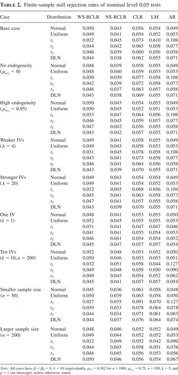
Table 2 presents the size results. The two rank CLR tests perform noticeably better in terms of size than the nonrank CLR, LM, and AR tests. Nine different cases are considered with six different distributions for each case. Over the 54 trials, the range of null rejection rates for each test is WS-RCLR: [0.027, 0.052]; NS-RCLR: [0.033, 0.051]; CLR: [0.047, 0.091]; LM: [0.042, 0.070]; and AR: [0.049, 0.127]. For the two rank tests, the majority of rejection rates are in the desired [0.040, 0.050] range, which corresponds to no overrejection and sufficiently small underrejection as to minimize the power loss. In particular, 44/54 for WS-RCLR and 38/54 for NS-RCLR are in this range. In contrast, for the nonrank tests a small number of rejection rates are in this desired range: 1/54 for CLR, 3/54 for LM, and 11/54 for AR. Not surprisingly, the largest overrejections for the nonrank tests occur for the thickest tailed distributions. If one widens the range to [0.04, 0.06], which includes overrejection by a small amount, then the RCLR tests still outperform the CLR and AR tests, but the LM test performs best of all. The numbers of cases in this range are 44/54 for WS-RCLR, 39/54 for NS-RCLR, 33/54 for CLR, 49/54 for LM, and 29/54 for AR.
Finite-sample null rejection rates of nominal level 0.05 tests

6.3. Power Comparisons
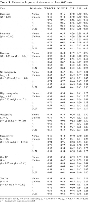
Table 3 presents the power results. The general pattern of finite-sample power in Table 3 reflects that of asymptotic power given in Table 1. In particular, the NS-RCLR and CLR tests have comparable power for the normal distribution, the NS-RCLR test has higher power than the CLR test for the uniform distribution in many cases and much higher power for the thick-tailed distributions. This occurs in the base case and in the variations of the base case. For example, in the base case with two β values the (average) power of the NS-RCLR test for the t2 distribution is 0.67 compared to 0.46 for the CLR test. The WS-RCLR and NS-RCLR tests have similar power with the NS-RCLR test having slightly higher power for the normal distribution, noticeably higher power for the uniform distribution, and slightly worse power for the thick-tailed distributions. The LM test has similar power to the CLR test, but with lower power in the weaker IVs case with normal distribution and slightly higher power for the heavy-tailed distributions. The AR test has significantly lower power than the other tests except in the case with k = 1.
Finite-sample power of size-corrected level 0.05 tests

In sum, the NS-RCLR test has power that essentially dominates that of the (nonrank) CLR, LM, and AR tests. Its power is comparable to that of the CLR and LM tests for the normal distribution and higher for the other distributions, especially the thick-tailed ones. The power of the WS-RCLR test is similar to that of the NS-RCLR test.
APPENDIX: Proofs
The proofs of Lemmas 1–5 and Corollary 1 are given at the end of the Appendix, as is the description of the numerical calculation of asymptotic power under weak IVs.
The proofs of Theorems 1(i) and 2(i) rely on the following lemmas. Lemma 6 follows from results of Koul (1970) and Hájek and Sidák (1967).
LEMMA 6. Let

, where
(i) ri(t) is the rank of Qi − di′t among {Qj − dj′t : 1 ≤ j ≤ n} for a constant vector t ∈ Rδd,
(ii) {Qi : i ≥ 1} is a sequence of i.i.d. random variables with absolutely continuous strictly increasing df H and absolutely continuous and bounded density h that satisfies I(h) < ∞,
(iii) {ci : i ≤ n,n ≥ 1} and {di : i ≤ n,n ≥ 1} are triangular arrays of nonrandom δc-vectors and δd-vectors, respectively (with dependence of ci and di on n suppressed for brevity), that satisfy

, and

and likewise with ci − cn replaced by di − dn, where

and

, and
(iv) the score function φ satisfies Assumption 3.
Then,
(a) for all ε > 0 and b < ∞,

where

(b) for any sequence of random δd-vectors

for which

,

(c)

.
Remarks.
(a) Lemma 6(a) is an extension of Theorem 2.1 and Lemma 2.3 of Koul (1970) from scalar constants ci and di to vectors. As Koul (1970, p. 1280) notes, his proof of these results goes through for this extension with virtually no changes. Lemma 6(b) follows from part (a). Lemma 6(c) follows from the proofs of the Hájek and Sidák (1967) Theorem V.1.5a (p. 160), Theorem VI.1.6a (p. 163), and Lemma VI.1.6a (p. 164), which show that in the scalar ci case

and

, respectively, where anφ(i) = E(φ(H(Q1))|r1(0) = i).
(b) The expression for

on p. 1277 of Koul (1970) is correct, but the expression for

given on p. 1278 (which is of the form given previously) contains a typo—a minus sign is missing. Also, the proof of Theorem 2.1 of Koul (1970) contains a typo that could be confusing to the reader. The term φ(qn) that appears at the end of the expression on the first two lines of the first equation on p. 1276 should be φ′(qn) in both places.
(c) We do not require φ to satisfy the second condition of (i) on p. 1274 of Koul (1970) because this is a normalization condition that implies that φ(½) = 0 which is not needed for his Theorem 2.1 or Lemma 2.3. It is needed for his n1/2Sn(0) to have an asymptotic normal distribution. We do not require it for n1/2Ψn(0) to have an asymptotic normal distribution because we consider demeaned constant vectors ci − cn, which yields n1/2Ψn(0) invariant to additive constants in φ, whereas Koul (1970) does not.
The next lemma is used to establish the probability limit of

.
LEMMA 7. Suppose
(i) {(Q1i,Q2i) : i ≥ 1} is an i.i.d. sequence of random (m + 1)-vectors with Q1i ∈ R,
(ii) (Q1i,Q2i) has an absolutely continuous and bounded joint df HQ1,Q2 that satisfies sup(q1,q2)|∂HQ1,Q2(q1,q2)/∂q1| < ∞,
(iii) E∥Q2i∥ < ∞,
(iv) ri(t) is the rank of Q1i − di′t among {Q1j − dj′t : j ≤ n}, where t ∈ Rδd,
(v) {di : i ≤ n,n ≥ 1} is a triangular array of nonrandom δd-vectors that satisfies

, and
(vi) the score function φ satisfies Assumption 3.
Then,
(a) for all b < ∞,

(b) for any sequence of random δd-vectors

for which

,

(c)

, where HQ1 is the df of Q1i.
Remark. Lemma 7(a) follows from arguments similar to those used to prove Lemma 2.2 in Koul (1970), which was originally proved, under different assumptions, as Theorem 3.1 in Koul (1969). The result established in Lemma 7(a) is different from the results established in Koul (1969, 1970), but the idea of the argument is essentially the same. The results in Koul (1969, 1970) are for a linear regression model with deterministic regressors. Hence, using our notation, the results in Koul (1969, 1970) are restricted to the case where {Q2i : i ≤ n} are nonrandom real numbers and {(Q1i,Q2i) :i ≤ n} and {di : i ≤ n} satisfy the relation imposed by a linear regression equation. Hence, the conditions in Lemma 7(a) generalize those in Lemma 2.2 of Koul (1970). On the other hand, Lemma 2.2 of Koul (1970) establishes that the left-hand side in Lemma 7(a) is op(n−1/2), which is a stronger result than that given in Lemma 7(a).
Let Φ be the n-vector with ith element given by φ(Ugi) = φ(G(ui + (β − β0)′v2i)).
LEMMA 8. Under Assumptions 1–3 and 4W,
(i) n−1/2Z′Rφ = n−1/2Z′(Φ + ZC[ell ]g,β−β0φ cφ1/2n−1/2) + op(1),
(ii) Snφ = (Z′Z)−1/2Z′(Φcφ−1/2 + ZC[ell ]g,β−β0φn−1/2) + op(1),
(iii) n−1Z′Z → DZ > 0, and
(iv) n−1/2Z′[(Φcφ−1/2 + ZC[ell ]g,β−β0φn−1/2) : Y2] →d [Nφ : N2].
LEMMA 9. Under Assumptions 1–3 and 4W,
(i)

and
(ii)

.
LEMMA 10. Under Assumptions 1–3 and 4S,
(i) n−1/2Z′Rφ = n−1/2Z′(Φ + ZΠ[ell ]f,Bφ cφ1/2n−1/2) + op(1),
(ii) Snφ = (Z′Z)−1/2Z′(Φcφ−1/2 + ZΠ[ell ]f,Bφn−1/2) + op(1), and
(iii) n−1Z′[Φ : Y2] →p DZ [0k : Π].
LEMMA 11. Under Assumptions 1–3 and 4S,
(i)

and
(ii)

.
The following lemma gives sufficient conditions for an i.i.d. sequence to satisfy Assumptions 2(d) and 4S(h) a.s.
LEMMA 12. Suppose {ψi : i ≥ 1} is an i.i.d. sequence of nonnegative random variables with Eψi1+δ < ∞ for some δ > 0. Then,
(i)

and
(ii) maxi≤n ψi/n → 0 a.s.
The last lemma is a Glivenko–Cantelli theorem for triangular arrays of random variables, which is used in the proof of Lemma 7. It is proved by verifying the conditions in Pollard (1990, Thm. 8.3).
LEMMA 13. Suppose
(i) {(Q1i,Q2i) : i ≥ 1} is an i.i.d. sequence of random (m + 1)-vectors with Q1i ∈ R and
(ii) {di : i ≥ 1} is any sequence of nonrandom δd-vectors.
Then, for any b < ∞,

where

The proofs of Lemmas 7–13 are given after the proofs of Theorems 1 and 2.
Proof of Theorem 1. Lemma 9 and Assumption 4W(e) imply that

This, Lemma 8, the continuous mapping theorem, and the definitions of (Snφ,Tnφ) and (S∞φ,T∞φ) combine to establish part (i).
Independence of S∞φ and T∞φ is implied by zero covariance between the normal variates Nφ and [Nφ : N2]Ωφg−1H. The latter holds by the following argument. Let Nφ,j, N2,[ell ], and DZ,j[ell ] denote the jth element of Nφ, the [ell ]th row of N2, and the (j,[ell ]) element of DZ, respectively. Let e1 denote an m + 1-vector of ones. The covariance between Nφ,j and the [ell ]th row of [Nφ : N2]Ωφg−1H for j,[ell ] = 1,…,k is

Parts (ii)–(iv) of the theorem follow immediately from part (i) and the continuous mapping theorem. █
Proof of Theorem 2. The result Snφ →d Sf∞φ of part (i) follows from Lemma 10(ii), Lemma 8(iii) (which does not rely on Assumption 4W), and the Lindeberg CLT applied to n−1/2Z′Φcφ−1/2. The CLT applies by the same argument as given in the proof of Lemma 8(iv) subsequently.
The result n−1/2Tnφ →d αTφ (or n−1/2Tnφ →p αTφ) is established as follows:

where the second equality holds because Lemma 11 and Assumption 4S(g) imply that

, the third equality holds by Lemma 8(iii) and Lemma 10(ii), the fourth equality holds by Lemma 10(iii), and the fifth equality holds because [0k : Π] = Π[0m : Im] = ΠH′. The convergence of (Snφ,n−1/2Tnφ) holds jointly because αTφ is a constant.
Parts (iii) and (iv) follow immediately from part (i) using the continuous mapping theorem noting that αTφ′αTφ is pd by Assumptions 2(c), 4S(b), and 4S(g).
We now prove part (ii). Given the definition of RLRnφ in (3.8) and the result of Theorem 2(iii), it suffices to show that

For notational simplicity, let [S : T] denote [Snφ : Tnφ] and let Tj ∈ Rm+1 denote the jth column of T for j = 1,…,m. We rotate [S : T] by an orthogonal matrix B ∈ R(m+1)×(m+1) whose first column, b1, is designed to be such that [S : T]b1 = d1S⊥, where d1 is a positive scalar that equals 1 + op(1). Then, we have

and the (1,1) element of the matrix on the right-hand side equals λ12d12S⊥′S⊥.
Let bj denote the jth column of B and let bij denote the (i,j)th element of B. Define

where d1 is a constant such that b1′b1 = 1. Next, we define the orthogonal vectors {bj : j = 2,…,m + 1} via the Gramm–Schmidt procedure applied to the vectors b1,e2,…,em+1, where ej is the jth elementary vector (whose jth element is one and whose other elements are zero). We have

and so on, where dj is the constant that yields ∥bj∥ = 1 for j = 1,…,m.
The constants {dj : j = 1,…,m + 1} satisfy

and so on, using Theorem 2(i) and the fact that

and so on.
Let

be such that ∥λ∥ = 1. Then, we have

The cross-product summand of J(λ) in (A.10) equals

using S⊥′T = 0, (S⊥′S)2 ≤ (S⊥′S⊥)S′S ≤ (S′S)2 = Op(1), |bij| ≤ 1, and d1 = 1 + op(1). For the third summand J3(λ) of J(λ), we have

Combining this with (A.8), (A.9), S⊥′T = 0, S⊥ = Op(1), and n−1/2T →p αTφ (by part (i) of the theorem), we obtain

where αTφ′αTφ is pd by Assumptions 2(c), 4S(b), and 4S(g).
Let

be an m + 1-vector that minimizes J(λ) over λ ∈ Rm+1 such that ∥λ∥ = 1. If

, then

by (A.10)–(A.13) and S⊥′S⊥ = Op(1) by part (i) of the theorem.
On the other hand, suppose that

and

; then |λ1*| = 1 + op(1),

This contradicts the assumption that λ* minimizes J(λ) over λ such that ∥λ∥ = 1 because a different choice of λ, namely, λ such that

, yields a smaller value J(λ) as indicated in (A.14).
Next, suppose that

. Then,

by (A.10)–(A.13). In particular, for some ε > 0 and some (infinite) subsequence {[ell ]n} of {n}, P(J3(λ*) > [ell ]nε) > ε when the sample size is [ell ]n for all n ≥ 1. Again this is a contradiction, because a different choice of λ, namely, λ such that

, yields a smaller value J(λ), namely, one that is Op(1) as indicated in (A.14). We conclude that

must satisfy

, and hence (A.14), (A.4), (A.5), and (A.10) combine to establish the result of part (ii). █
Proof of Lemma 7. Because E∥Q2i∥ < ∞, given any ε > 0, there exists a constant cε < ∞ such that

Hence, using the boundedness of φ, say, by C, and Markov's inequality, we have for any η > 0 and ε > 0,

Therefore, without loss of generality, we can assume that Q2i is bounded.
Define

Note that

Now, we have

Therefore, using the triangle inequality,

where, for b ≥ 0,

Now, by Lemma 13,

This implies that A1n(b) →p 0 and A1n(0) →p 0, because φ is absolutely continuous, Q2i is bounded, and 0 ≤ A1n(0) ≤ A1n(b).
Using the triangle inequality again, we have A2n ≤ B1n + B2n, where


To bound B1n and B2n, we write

The first and last terms on the right-hand side converge to zero a.s. by Lemma 13. The second term on the right-hand side converges to zero because it equals

where t* lies between 0 and t, the first equality holds by a mean-value expansion around t = 0, and the second equality holds because ∂HQ1,Q2/∂q1 is bounded (Assumption 4W(d)) and

. Therefore, using the boundedness of φ and Q2i, we have B2n →p 0.
Equation (A.27) and a mean-value expansion yield B1n →p 0 because φ has a bounded first derivative by Assumption 3(a). In consequence, A2n →p 0, which completes the proof of part (a).
Part (b) of the lemma follows from part (a) using a standard argument.
To prove part (c), as in part (a), we can assume that Q2i is bounded without loss of generality. We have

where the first equality holds by (A.21) with t = 0, the second equality holds because A1n(0) →p 0, the third equality holds by (A.20), and the fourth equality holds because n/(n + 1) → 1, Q2i is bounded, and φ has a bounded derivative. █
Proof of Lemma 8. We prove part (i) first. Using (2.1) and Assumption 4W(a),

In consequence, we apply Lemma 6 with

Note that cn = Zn = 0 because Xi contains an intercept by Assumption 2(b) and Z′X = 0 by construction. The required conditions of Lemma 6 on di are satisfied by Assumption 2. The assumptions on Qi are satisfied by Assumptions 1(a) and 4W(b) and (c). The condition

holds by Assumption 4W(f).
We now verify the conditions of Lemma 6 on ci = Zi. By construction,

, where

by Assumption 2(c). In consequence, by standard arguments using Assumptions 2(c) and (d), we obtain

and limn→∞ max1≤i≤n ∥Zi∥2/n = 0. Hence, all of the conditions of Lemma 6 hold.
Now, using (A.30) and Zn = 0,

equals

The second summand is zero because Z′X = 0. The first summand equals n−1Z′ZC(β − β0) because

. Hence, by Lemma 6(b), we have

(By definition, n1/2Ψn(0) = n−1/2Z′Rφ0, where Rφ0 is the n-vector whose ith element is φ(Ri/(n + 1)) and Ri is the rank of ui + (β − β0)′v2i in {uj + (β − β0)′v2j : j ≤ n}.)
Finally, Lemma 6(c) implies that

Combining (A.32), (A.33), and the definition of [ell ]g,β−β0φ in (4.5) establishes Lemma 8(i).
Lemma 8(ii) follows from part (i) and Assumption 2(c).
Lemma 8(iii) follows from Assumption 2(c) and

. Positive definiteness of DZ follows from that of D.
Lemma 8(iv) follows from the Lindeberg CLT for triangular arrays applied to n−1/2Z′[Φcφ−1/2 : Y2 − EY2] plus the facts that

for arbitrary fixed nonzero vectors μ1 ∈ Rk and μ2 ∈ Rm+1. Note that EZ′Φ = 0 because Zn = 0 and Eφ(Ugi) does not depend on i.
The Lindeberg condition is verified for n−1/2μ1′Z′[Φcφ−1/2 : Y2 − EY2]μ2 (for μ1 and μ2 as before), as follows. Let ζi = (φ2(Ugi)cφ−1/2,v2i′)μ2 ∈ R. For any ε > 0,

where the inequality uses (μ′Zi)2 ≤ maxj≤n(μ′Zj)2 in the indicator function and the convergence to zero holds by Assumption 2, E∥v2i∥2 < ∞ (by Assumption 1(b)), Eφ2(Ugi) < ∞ (by Assumption 3), and the dominated convergence theorem. █
Proof of Lemma 9. We prove part (i) first. Let V2 be the n × m matrix whose ith row is v2i′. Using Z′X = 0, we have

We have n−1V2′Z →p 0 and n−1V2′X →p 0 because they have mean zero and variance O(n−1) by Assumptions 1 and 2(a) and (c). Assumption 2(c) implies that (n−1Z′Z)−1 and (n−1X′X)−1 are Op(1). Lemma 8(i) and (iv) implies that n−1/2Z′Rφ = Op(1). These results combine to show that the second term on the right-hand side of (A.36) is op(1). Next, we have

for some constant C < ∞, using the triangle inequality, the boundedness of φ, and Assumption 2(c). This result and the others given previously imply that the third term on the right-hand side of (A.36) is op(1). Hence,

.
We apply Lemma 7 with Q1i = ui + (β − β0)′v2i, Q2i = v2i, and di and

as in (A.30) to get

The conditions of Lemma 7 on

, di, and (Q1i,Q2i) hold by Assumptions 4W(f), 2(c), and 4W(d), respectively.
Next, we prove part (ii). For simplicity, we replace n − k − p by n in the definition of

. We have

where V2 denotes the n × m matrix whose ith row is v2i′, n−1V2′V2 →p Ω22 by Kolmogorov's law of large numbers for i.i.d. random variables, and n−1Z′V2 →p 0 and n−1X′V2 →p 0 because they have mean zero and variances that are O(n−1) by Assumptions 1 and 2(a) and (c). █
Proof of Lemma 10. We prove part (i) first. It suffices to show that (Snφ,n−1/2Tnφ) →d (Sf∞φ,αTφ) conditional on an {εi : i ≥ 1} sequence that satisfies certain properties, and that {εi : i ≥ 1} sequences satisfy these properties with probability one. Because conditional probabilities are bounded by zero and one, this implies that (Snφ,n−1/2Tnφ) →d (Sf∞φ,αTφ) unconditionally by the bounded convergence theorem. The desired properties are


Conditions (A.40) and (A.41) hold a.s. by Assumption 4S(d), Lemma 12(ii), and Kolmogorov's strong law of large numbers. Conditions (A.42) and (A.43) hold a.s. by Assumptions 4S(d) and (h) and the strong law of large numbers of Theorem 5.2.1 of Chow and Teicher (1978, p. 121) applied with αn = 2. Consequently, sequences {εi: i ≥ 1} that satisfy (A.40)–(A.43) occur with probability one.
Using (2.1) and Assumptions 4S(a)–(c), we have


Let ζn = (1 + ρ′Bn−1/2)−1. Because ζn > 0 for n sufficiently large,

are equal to the ranks of the i.i.d. random variables {ui : i ≤ n} plus the terms

Hence, we apply Lemma 6, conditional on an {εi : i ≥ 1} sequence that satisfies (A.40)–(A.43), with

The assumptions of Lemma 6 on Qi are satisfied by Assumptions 1 and 4S(e). The required conditions for ci are verified by the same argument as in the proof of Theorem 1. The assumptions on di are satisfied by Assumption 2, (A.40), and (A.41). The assumptions on

are satisfied by Assumption 4S(i) because ζn → 1.
Using the definitions of ci, di, and

,

equals

The first term in (A.47) equals Z′ZΠB + o(1) because ζn → 1. The second term is zero because Z′X = 0. The third term equals

using (A.42), (A.43), and Assumption 2(c). Hence, by Lemma 6(b) and (c), we have

which establishes part (i).
Lemma 10(ii) follows from part (i) and Assumption 2(c).
To establish Lemma 10(iii), we have

where V2 denotes the n × m matrix whose ith row is v2i′ and using n−1Z′V2 →p 0 because its mean is zero and its variance is O(n−1) by Assumptions 1 and 2(a) and (c).
In addition, we have

where the equality holds because EΦ is proportional to 1n and Z′1n = 0 and the convergence to 0 holds by the strong law of large numbers referenced in the previous paragraph. █
Proof of Lemma 11. We prove part (i) first. By the same argument as in the proof of Lemma 9(i), but with Lemma 8 replaced by Lemma 10, we have

. As in the proof of Lemma 10(i), it suffices to show the result conditional on an {εi : i ≥ 1} sequence that satisfies certain properties and that {εi:i ≥ 1} sequences satisfy these properties with probability one. In the present case, we need the property

Condition (A.52) holds a.s. by Kolmogorov's strong law of large numbers using Assumption 4S(d).
Lemma 7 applied conditional on a sequence {εi : i ≥ 1} that satisfies (A.52), with (Q1i,Q2i) = (ui,v2i) and di and

as in (A.46), gives

The conditions of Lemma 7 on

, di, and (Q1i,Q2i) hold by Assumption 4S(i), condition (A.52) and Assumptions 2(c) and (d), and Assumption 4S(f), respectively.
The proof of part (ii) is the same as for Lemma 9(ii). █
Proof of Lemma 12. Part (i) holds because

implies that

Part (ii) holds because the result of part (i) and Kronecker's lemma (see, e.g., Chow and Teicher, 1978, p. 111) imply that

Hence,

In turn, this gives n−1 maxi≤n ψi → 0 a.s. █
Proof of Lemma 13. We prove the lemma by verifying the conditions of Theorem 8.3 in Pollard (1990). To match the notation in Pollard (1990), view the sequence {(Q1i,Q2i) : i ≥ 1} as depending on ω ∈ Ω, where the probability space is

, and let (Q1i,Q2i)(ω) denote the ith element of this sequence. Also, view the sequence of independent processes

for i ≥ 1 as a sequence of independent processes indexed by

:

Each of the processes hni(ω;τ) has envelope Hni(ω) = 1 ∀ω ∈ Ω, and these envelope functions satisfy

which is the first condition of Theorem 8.3 of Pollard (1990).
Now, we verify that the processes

and the envelope functions {Hni(ω) = 1 ∀ω ∈ Ω} for i ≥ 1 satisfy the second condition of Theorem 8.3 of Pollard (1990). For each ω, define the sets

for some α ∈ Rn.
Denote the largest number κ for which there exist points in a subset of a metric space T with d(ti,tj) > ε, for i ≠ j, by D(ε,T). The number D(ε,T) is called the packing number. Denote the [ell ]1 distance in Rn by

.
By Definition 7.9 of Pollard (1990),

for i ≥ 1 is manageable with respect to the envelopes {Hni(ω) = 1 ∀ω ∈ Ω} for i ≥ 1 if there exists a function λ(ε) such that
- ,

- for 0 < ε ≤ 1, all ω ∈ Ω, all vectors of nonnegative weights α, and all n. (Because Hni(ω) = 1 ∀ω we have that |α [odot ] H|1 = |α|1, where H = (Hni(ω),…,Hnn(ω)).)


The second condition of Theorem 8.3 of Pollard (1990) is that

for i ≥ 1 is manageable with respect to the envelopes {Hni(ω) = 1 ∀ω ∈ Ω} for i ≥ 1.
For any ω, the class

belongs to a larger class of functions

defined by

The collection of all cells (−∞,c1] × (−∞,c2]m has VC-index equal to (m + 1) + 1, which implies that the class of indicator functions

has VC-index equal to (m + 1) + 1 also (see van der Vaart and Wellner, 1996). From Theorem 2.6.7 in van der Vaart and Wellner (1996), it follows that there exist constants A1 and W such that

where

is the smallest number of closed balls with radius ε/2 that covers

. The number

is called the covering number of

. Because

and

for every n and ω, it follows that there exist constants A2 and W,

Now, using an argument similar to the one used in the proof of Theorem 4.8 of Pollard (1990), we can show that for all n and ω, there exist constants A3 and W such that

Take

to be the set of rescaled coordinates

Let h1* and h2* in

be rescaled coordinates of h1 and h2 in

. Then,

Hence,

Now, we have

Therefore, (A.61) holds with A3 = 2WA2. This establishes that

is manageable with respect to the envelopes {Hni(ω) = 1 ∀ω ∈ Ω}. Theorem 8.3 of Pollard (1990) then gives

which gives the result of the lemma. █
Proof of Lemma 1. By the definition of

, we have

using y2i = Π′Zi + ξ′Xi + v2i and X′Z = 0. Hence, we obtain

Assumption 2(c) implies that (n−1X′X)−1 = D11−1 + o(1). The second multiplicand of the first term on the right-hand side of (A.68) is asymptotically normal by the Lindeberg central limit theorem using Assumptions 1 and 2 and Eui2 < ∞. The Lindeberg condition is verified by an argument analogous to that in (A.35), where E(ui + (β − β0)′v2i)2 < ∞ by Assumption 1(b) and Eui2 < ∞. Thus, the first term on the right-hand side of (A.68) is O(1). Next, we have

where the first equality holds by the definition of ξ stated following (2.3), the second equality holds by Assumption 4W(a), and the last equality holds by Assumption 2(c). Assumption 4W(b) states that β − β0 is a constant. Hence, n1/2(ξ − ξ1)(β − β0) = O(1), which completes the proof of the lemma. █
Proof of Corollary 1. We have

where FT∞φ(·) is the df of T∞φ, the convergence holds by Theorem 1(i) and the continuous mapping theorem, the second equality holds by the independence of S∞φ and T∞φ, and the last equality holds by the definition of κLR,α(t′t,k,m) in (3.10) and the fact that S∞φ ∼ N(0,Ik) under the null by (4.6). █
Proof of Lemma 2. The proof is very similar to that of Theorem 1 with

in place of Φcφ−1. First, by the same proof as for Lemma 9(ii) but with (Y2,V2) replaced by (Y,V), we get

, where V is the n × (m + 1) matrix with ith row equal to vi′. This implies

and

. Next, we need the following analogues of Lemma 8(i), (ii), and (iv):


where (A.71) holds by (2.1), (2.3), Assumption 1(a), and Z′X = 0, (A.72) holds by (A.71) and

, and (A.73) holds by the same proof as that of Lemma 8(iv) (given earlier) except with Φcφ−1/2, [ell ]g,β−β0φ, and φ(Ugi)cφ−1/2 replaced by Vb0σg−1, (β − β0)σg−1, and v2i′b0σg−1, respectively, and with E(v2i′b0)2 < ∞ by the assumption that Ω is well defined. Given these analogues of Lemma 8(i), (ii), and (iv), the rest of the proof of Lemma 2 is the same as that of Theorem 1. █
Proof of Lemma 3. We establish part (i) first. Let σL2 denote the variance of the df L. Because φ(x) = L−1(x), cφ = σL2 by change of variables. Also, we have

Combining these results gives the result of part (i):

Part (i) implies that νφg = νg, and so Ωφg = Ωg and part (ii) holds.
For part (iii), we have

where the second equality holds by change of variables with y = G−1(x), the third and last equalities hold by (A.74), and the fourth equality holds by integration by parts. Combining (A.76) with cφ = σL2 establishes part (iii).
Part (iv) follows from parts (ii) and (iii) and the definitions of Nφ, N1, S∞φ, S∞, T∞φ, and T∞. █
Proof of Lemma 4. The proof is like that of Theorem 2 with

in place of Rφcφ−1. By essentially the same proof as for Lemma 9(ii) but with (Y2,V2) replaced by (Y,V), we get

. Under Assumption 4S(a), we have

In consequence,

We need the following analogue of Lemma 10(ii):

which holds by (2.1), (2.3), Assumption 1(a), Z′X = 0, and

. Next, an analogue of (A.3) holds with

, and n−1Z′Rφ replaced by

, and n−1Z′Yb0 = n−1Z′(Vb0 + ZΠBn−1/2), respectively, using the result that

and the fact that n−1Z′Vb0 →p 0 because its mean is zero and its variance is O(n−1). Given these analogues of Lemma 10(ii) and (A.3), the rest of the proof of Lemma 4 is the same as that of Theorem 2. █
Proof of Lemma 5. The proofs of parts (i)–(iii) are analogous to those of parts (i)–(iii) of Lemma 3. Part (iv) follows from parts (ii) and (iii) and the definitions of Sf∞φ, Sf∞, αTφ, and αT. █
Proof of an Alternative Expression for Tn. We now provide a proof of (3.6), which gives an alternative expression for Tn from its definition in (2.6). Let

. Straightforward calculations yield

Using the definition of Tn in (2.6), we have

where the second equality uses (A.80). The right-hand side of (A.81) is the expression in (3.6). █
Asymptotic power calculations.
Next, we describe the simulation method used to calculate the weak IV asymptotic power reported in Table 1. The first step is to compute ξ(φNS,g) and ξ(φWS,g) when g is the density of ui + βv2i for v2i defined in (4.18) and ui and εi are independent with distribution F. The idea is to use the fact that the Hodges–Lehmann estimator of location based on φ (which is defined, e.g., in Hettmansperger, 1984, eqn. (2.8.12), p. 99) has asymptotic variance equal to 1/ξ(φ,g) (see Hettmansperger, 1984, Thm. 2.6.5 and eqn. (2.9.4), pp. 76, 105). We compute the Hodges–Lehmann estimators based on φNS and φWS for 30,000 independent samples of a location model with density g and sample size 100,000. This yields 30,000 Hodges–Lehmann estimates

and

. The reciprocals of the sample variances of these estimates yield estimated values of ξ(φNS,g) and ξ(φWS,g), denoted

and

.
The second step is to compute the matrices ΩφNSg, ΩφWSg, and Ωg and the scalar σg2 defined in (4.1) and (4.10). The df G(x) is approximated by the empirical df of 100,000 i.i.d. observations with distribution G (independent of the preceding random variables), call it

. Using the same observations, σg2 is estimated by the sample variance, denoted

. Next, νφ,g is estimated by

, where R = 40,000 for all distributions except the uniform, R = 100,000 for the uniform distribution,

,

,

,

and

are independent with distribution F, are independent of

, and are i.i.d. across i = 1,…,R, and φ = φNS,φWS. The term νg is estimated by the sample covariance between

and

, denoted

, and ω22 is estimated by the sample variance of

, denoted

. The matrices

,

, and

are constructed using

,

,

, and

.
The third step is to compute 5,000 independent observations of (i) two independent k-variate normals

with covariance matrices equal to Ik and means given by

and

, respectively, for φ = φNS,φWS, where e1 = (1,0,…,0)′ ∈ Rk and e2 = (0,1)′, and (ii) two independent k-variate normals

with covariance matrices equal to Ik and means as in (i) but with

in place of

. The same normal random variables were used for

,

, and

—just the means are different.
The last step is to compare each of the 5,000 WS-RCLR, NS-RCLR, CLR, LM, and AR test statistics based on

,

, and

with the appropriate conditional critical value (determined by simulation) or unconditional critical value to determine whether the test rejects the null hypothesis. The fraction that rejects the null hypothesis is the reported power in Table 1.