Configuration and design

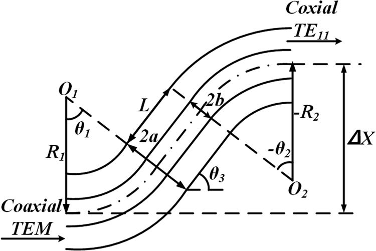
The structure of the dual-bend mode converter to be designed is shown in Fig. 1. It consists of a straight waveguide and two-waveguide bends. The curvature radii and bending angles of the two bends are R ₁, −R ₂, θ ₁, and −θ ₂, respectively, where the minus sign indicates that the two bends are opposite to each other. The straight waveguide with length as L is designed to realize an offset Δx from the axis of the output port to the axis of the input port, which is shown by equation (1).

(1)$$\Delta x = R_1(1-\cos \theta _1)-R_2(1-\cos \theta _2) + L\sin \theta _3$$

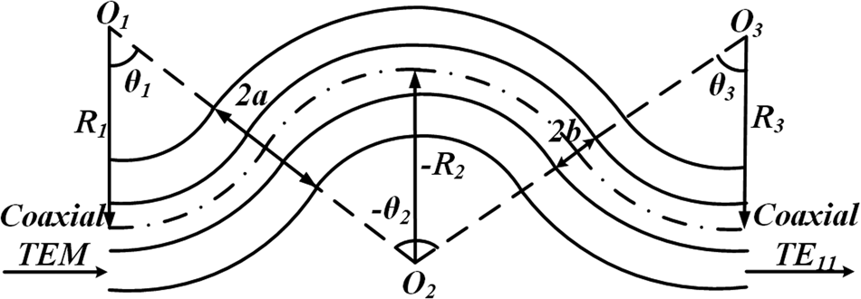
As shown in Fig. 2, the tri-bend mode converter is formed with three bends, the curvature radii are R ₁, –R ₂, and R ₃, and bend angles are θ ₁, –θ ₂, and θ ₃, respectively. All the three bends are connected back-to-back at the tangent points in order to prevent the junction producing additional coupling or reflections. Different from the dual-bend mode converter, the input and output ports of the tri-bend mode converter are aligned on the same axis, which improves the radial compactness of the whole system.

Fig. 1.

Geometry sketch of the dual-bend mode converter.

Fig. 2.

Geometry sketch of the tri-bend mode converter.

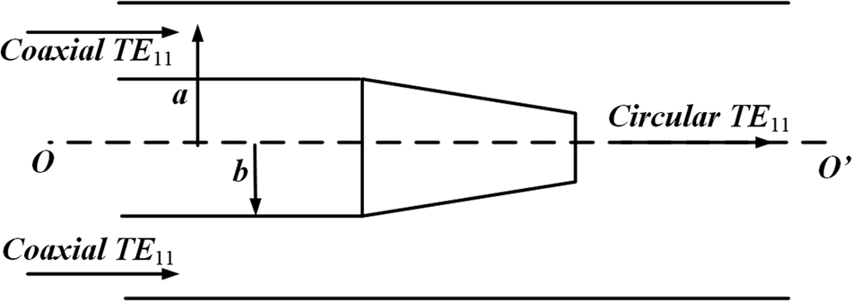
Additionally, for certain output requirements of circular TE₁₁ mode, the transformation from coaxial TE₁₁ mode to circular TE₁₁ mode can be realized by a cone at the end of the inner conductors of both converters as shown in Fig. 3 [Reference Yuan, Liu, Zhong and Qian12]. Through the optimization of the length and the radius of the top, the introduction of the cone will not affect the output modes of the converters and the return loss at the central frequency can be reduced to less than −30 dB.

Fig. 3.

Conversion structure between the coaxial waveguide and circular waveguide.

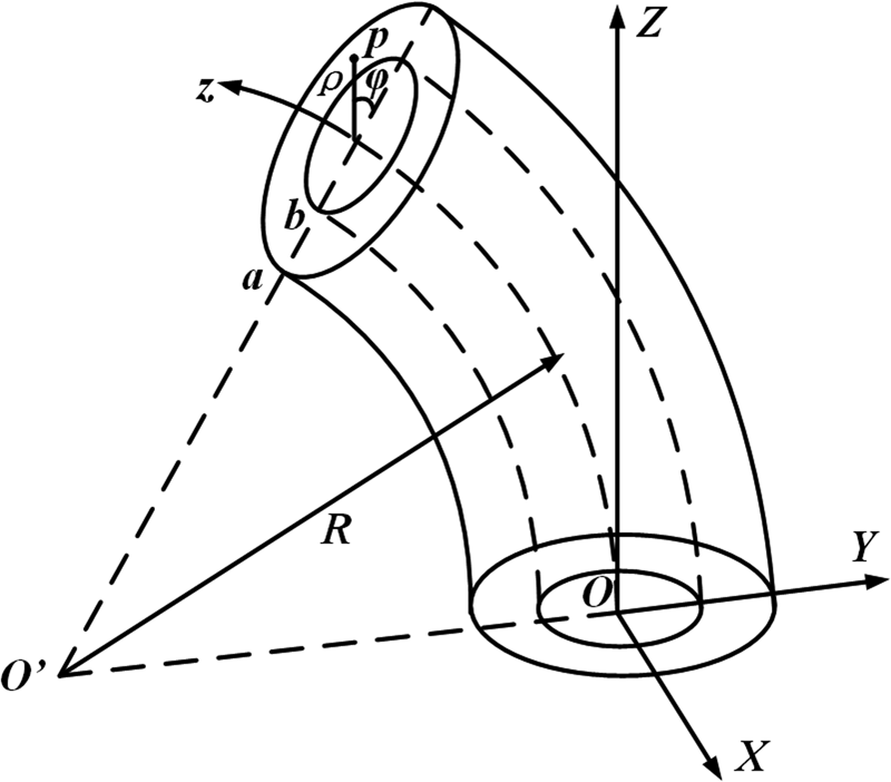
Mode coupling theory is an effective way to analyse the waveguide bend [Reference Li and Thumm13]. There already have been sufficient studies of the mode coupling inside the circular waveguide bend and rectangular waveguide bend [Reference Weisshaar, Goodnick and Tripathi14, Reference Blas, Gimeno, Boria, Esteban and Coves15]. However, few works have been performed on the mode coupling inside the coaxial waveguide bend. Therefore, in order to design the converters, the mode coupling and conversion due to curvatures in the coaxial waveguide bend are analysed. The coaxial waveguide bend is shown in Fig. 4, where the x-direction is normal to the bend plane, and the bend is assumed to be perfectly conducting. a, b is the outside and inside radius of the coaxial waveguide, respectively, and R is the curvature radius of the bend. A curvilinear coordinate (ρ, φ, θ) is established to facilitate the analysis, the transformation relation between the curvilinear coordinate and rectangular coordinate can be expressed as follows:

(2)$$\left\{ \matrix{X = \rho \sin \varphi \hfill \cr Y = (R + \rho \cos \varphi )\cos (z/R)-R \hfill \cr Z = (R + \rho \cos \varphi )\sin (z/R) \hfill} \right.$$

Hence, the scale factors can be easily derived according to [Reference Li and Thumm13]:

(3)$$h_1 = 1,\quad h_2 = \rho, \quad h_3 = 1 + (\rho \cos \varphi )/R$$

Based on the derived scale factors, the Maxwell's equations in the curvilinear coordinate can be written as equation (4), where E and H are the electrical field and magnetic field, respectively. E_T and H_T are the transverse field components, E _z and H _z are the longitudinal field components. ω is the circular frequency of the transmission wave.

(4)$$\left\{ \matrix{(\nabla \times {\bf E}) \times {\vec{a}}_z = \displaystyle{1 \over {h_3}}\displaystyle{{\partial ({\vec{a}}_z \times {\bf E}_{\bf T})} \over {\partial z}} \times {\vec{a}}_z-\displaystyle{1 \over {h_3}}\nabla _T(h_3E_z) \hfill \cr \quad = -j\omega \mu {\bf H}_{\bf T} \times {\vec{a}}_z \hfill \cr (\nabla \times {\bf H}) \times {\vec{a}}_z = \displaystyle{1 \over {h_3}}\displaystyle{{\partial ({\vec{a}}_z \times {\bf H}_{\bf T})} \over {\partial z}} \times {\vec{a}}_z-\displaystyle{1 \over {h_3}}\nabla _T(h_3H_z) \hfill \cr \quad = -j\omega \varepsilon {\bf E}_{\bf T} \times {\vec{a}}_z \hfill} \right.$$

Considering that waves inside the coaxial waveguide bend can be described by the field functions of the straight coaxial waveguide with the same cross section, the electrical and magnetic field in equation (4) are expanded in series of transmission TE waves and TM waves, which are shown in equations (5) and (6).

(5)$$\left\{ \matrix{E_z = -\displaystyle{\,j \over {\sqrt {\omega \varepsilon}}} \sum\limits_{nm} {\sqrt {\displaystyle{1 \over {\beta_{nm}}}}} (A_{nm}^ + -A_{nm}^- )\chi_{nm}^2 \Pi_{nm} \hfill \cr H_z = -\displaystyle{\,j \over {\sqrt {\omega \mu}}} \sum\limits_{nm} {\sqrt {\displaystyle{1 \over {\beta_{nm}^{^\ast}}}}} (A_{nm}^{{^\ast} +} + A_{nm}^{{^\ast}-} )(\chi_{nm}^{^\ast} )\Pi_{nm}^{^\ast} \hfill} \right.$$

(6)$$\left\{ \matrix{{\bf E}_{\bf T} = -\sum\limits_{nm} {\sqrt {\displaystyle{{\beta _{nm}} \over {\omega \varepsilon }}} } (A_{nm}^ + + A_{nm}^- )\nabla _T\Pi _{nm} + \sum\limits_{nm} {\sqrt {\displaystyle{{\omega \mu } \over {\beta _{nm}^\ast }}} } (A_{nm}^{\ast + } \hfill \cr \quad + A_{nm}^{\ast-} ){\vec{a}}_z \times \nabla _T\Pi _{nm}^\ast \hfill \cr {\bf H}_{\bf T} = -\sum\limits_{nm} {\sqrt {\displaystyle{{\omega \varepsilon } \over {\beta _{nm}}}} } (A_{nm}^ + -A_{nm}^- ){\vec{a}}_z \times \nabla _T\Pi _{nm} \hfill \cr \quad + \sum\limits_{nm} {\sqrt {\displaystyle{{\beta _{nm}^\ast } \over {\omega \mu }}} } (A_{nm}^{\ast + } -A_{nm}^{\ast-} ){\vec{a}}_z \times ({\vec{a}}_z \times \nabla _T\Pi _{nm}^\ast ) \hfill} \right.$$

where $A_{nm}^ \pm $ and $A_{nm}^{\ast \pm} $ denote the complex amplitudes of forward and backward coaxial TM_nm modes and coaxial TE_nm modes, respectively. β _nm and $\beta _{nm}^\ast $ are the propagation constants of coaxial TM_nm mode and coaxial TE_nm mode. Π_nm and $\Pi _{nm}^\ast $ are the hertz potentials of coaxial TM_nm mode and coaxial TE_nm mode, respectively.

Fig. 4.

Curvilinear coordinate of the coaxial waveguide bend.

Based on equations (4)–(6), the coupled-wave differential equations of the coaxial waveguide bend can be derived and are presented in equation (7).

(7)$$\hskip-2pt\left\{\!\! \matrix{\displaystyle{{dA_{{n}^{\prime}{m}^{\prime}}^ \pm } \over {dz}} = \!\mp j\beta _{{n}^{\prime}{m}^{\prime}}A_{{n}^{\prime}{m}^{\prime}}^ \pm \!\mp \!\!\sum\limits_{nm} \!{\left[\!\! \matrix{C_{({n}^{\prime}{m}^{\prime})(nm)}^ + A_{nm}^ \pm + C_{({n}^{\prime}{m}^{\prime})(nm)}^- A_{nm}^\mp \hfill \cr + C_{({n}^{\prime}{m}^{\prime})(\ast nm)}^ + A_{nm}^{\ast \pm } + C_{({n}^{\prime}{m}^{\prime})(\ast nm)}^- A_{nm}^{\ast\mp } \hfill} \!\!\right]} \hfill \cr \displaystyle{{dA_{{n}^{\prime}{m}^{\prime}}^{\ast \pm } } \over {dz}} =\! \mp j\beta _{{n}^{\prime}{m}^{\prime}}^\ast A_{{n}^{\prime}{m}^{\prime}}^{\ast \pm }\! \mp \! \sum\limits_{nm} \!{\left[ \!\!\matrix{C_{(\ast{n}^{\prime}{m}^{\prime})(\ast nm)}^ + A_{nm}^{\ast \pm } + C_{(\ast{n}^{\prime}{m}^{\prime})(\ast nm)}^- A_{nm}^{\ast\mp } \hfill \cr + C_{(\ast{n}^{\prime}{m}^{\prime})(nm)}^ + A_{nm}^ \pm + C_{(\ast{n}^{\prime}{m}^{\prime})(nm)}^- A_{nm}^\mp \hfill}\!\! \right]} \hfill} \right.$$

where $C_{({n}^{\prime}{m}^{\prime})(nm)}^ \pm $, $C_{({n}^{\prime}{m}^{\prime})(\ast nm)}^ \pm $, $C_{(\ast{n}^{\prime}{m}^{\prime})(\ast nm)}^ \pm $, and $C_{(\ast{n}^{\prime}{m}^{\prime})(nm)}^ \pm $ are the coupling coefficients between the transmission TM_nm mode and TM_n′m′ mode, TE_nm mode and TM_n′m′ mode, TE_nm mode and TE_n′m′ mode, and TM_nm mode and TE_n′m′ mode in the coaxial waveguide bend, respectively, and the positive and negative signs of the coupling coefficients stand for the same and opposite propagation directions of the two-coupled modes.

According to the rules of mode coupling, it is concluded that |n ^′ − n| = 1 is the precondition for the coupling of two modes. Obviously, coaxial TEM (TM₀₀) mode only couples with coaxial TM_1m′ and TE_1m′ modes. The differential equations then can be simplified to equation (8) and the corresponding coupling coefficients are strictly derived as follows:

(8)$$\left\{ \!\matrix{\displaystyle{{dA_{{\rm 00}}^ \pm } \over {dz}} = \mp j\beta _{{\rm 00}}A_{{\rm 00}}^ \pm \mp \sum\limits_m {\left[ \matrix{C_{\left( {{\rm 00}} \right)\left( {{\rm 1}m} \right)}^ + A_{{\rm 1}m}^ \pm + C_{\left( {{\rm 00}} \right)\left( {{\rm 1}m} \right)}^- A_{{\rm 1}m}^\mp \hfill \cr \quad + C_{\left( {{\rm 00}} \right)\left( {\ast{\rm 1}m} \right)}^ + A_{{\rm 1}m}^{\ast \pm } + C_{\left( {{\rm 00}} \right)\left( {\ast{\rm 1}m} \right)}^- A_{{\rm 1}m}^{\ast\mp } \hfill} \!\right]} \hfill \cr \displaystyle{{dA_{{\rm 1}{m}^{\prime}}^ \pm } \over {dz}} = \mp j\beta _{{\rm 1}{m}^{\prime}}A_{{\rm 1}{m}^{\prime}}^ \pm \mp \sum\limits_m {\left[ {C_{\left( {{\rm 1}{m}^{\prime}} \right)\left( {{\rm 00}} \right)}^ + A_{{\rm 00}}^ \pm + C_{\left( {{\rm 1}{m}^{\prime}} \right)\left( {{\rm 00}} \right)}^- A_{{\rm 00}}^\mp } \right]} \hfill \cr \displaystyle{{dA_{{\rm 1}{m}^{\prime}}^{\ast \pm } } \over {dz}} = \mp j\beta _{{\rm 1}{m}^{\prime}}^\ast A_{{\rm 1}{m}^{\prime}}^{\ast \pm } \mp \sum\limits_{{\rm 1}m} {\left[ {C_{\left( {\ast{\rm 1}{m}^{\prime}} \right)\left( {{\rm 00}} \right)}^ + A_{{\rm 00}}^ \pm + C_{\left( {\ast{\rm 1}{m}^{\prime}} \right)\left( {{\rm 00}} \right)}^- A_{{\rm 00}}^\mp } \right]} \hfill} \right.$$

(9)$$\eqalign{{\rm TEM mode}&\leftrightarrow {\rm T}{\rm M}_{1{m}^{\prime}}{\rm mode}: \cr C_{(1{m}^{\prime})(00)}^ \pm = \,&C_{(00)(1{m}^{\prime})}^ \pm \cr & \hskip-4pc = j\displaystyle{{\pi \left( {120\pi \omega \varepsilon \beta _{1{m}^{\prime}} \pm \omega ^2\varepsilon \mu } \right)\left[ \matrix{J_0\left( {v_{1{m}^{\prime}}{a \over b}} \right) \hfill \cr \quad N_0\left( {\nu _{1{m}^{\prime}}} \right)-N_0\left( {v_{1{m}^{\prime}}{a \over b}} \right)J_0\left( {\nu _{1{m}^{\prime}}} \right) \hfill} \right]} \over \matrix{2R\left( {\displaystyle{{v_{1{m}^{\prime}}} \over b}} \right)^2\sqrt {240\pi \omega \varepsilon \beta _{1{m}^{\prime}}\ln \left( {{a \over b}} \right)} \hfill \cr \quad \sqrt {{\left[ {({{J}^{\prime}}_1\left( {\nu _{1{m}^{\prime}}} \right))/{{J}^{\prime}}_1\left( {v_{1{m}^{\prime}}{a \over b}} \right)} \right]}^2-1} \hfill} }} $$

(10)$$\eqalign{{\rm TEM mode}&\leftrightarrow {\rm T}{\rm E}_{1{m}^{\prime}}{\rm mode :} \cr C_{(*1{m}^{\prime})(00)}^ + = \,&C_{(00)(*1{m}^{\prime})}^ + = j\displaystyle{{b\pi \left( {120\pi \omega \varepsilon \sqrt {\omega \mu } \pm \beta _{1{m}^{\prime}}^* \sqrt {\omega \mu } } \right)} \over {4R\mu _{1{m}^{\prime}}\sqrt {120\pi \beta _{1{m}^{\prime}}^* \ln \left( {{a \over b}} \right)} }} \cr & \times \displaystyle{\matrix{{J}^{\prime}_1\left( \mu _{1{m}^{\prime}} \right)\left[ N_0\left( \mu _{1{m}^{\prime}}{a \over b} \right) -N_0\left( \mu _{1{m}^{\prime}} \right) \right]\cr -{{N}^{\prime}}_1(\mu _{1{m}^{\prime}})\left[ {J_0\left( {\mu _{1{m}^{\prime}}{a \over b}} \right)-J_0\left( {\mu _{1{m}^{\prime}}} \right)} \right]} \over \sqrt {\matrix{\left[ ({J}^{\prime}_1\left( \mu _{1{m}^{\prime}} \right))/({J}^{\prime}_1(\mu _{1{m}^{\prime}}{a \over b})) \right]^2\cr \left[ 1-\left( 1/(\mu _{1{m}^{\prime}}{a \over b}) \right)^2 \right]-\left[ 1-\left( 1/\mu _{1{m}^{\prime}} \right)^2 \right]}}} } $$

where N ₀₍₁₎(x) and J ₀₍₁₎(x) are the ordinary Neumann function and Bessel function, respectively. $\mu _{1{m}^{\prime}}$ and $\nu _{1{m}^{\prime}}$ are the m′-th root of equations (11) and (12), respectively.

(11)$${J}^{\prime}_1(\mu _{1{m}^{\prime}}{a \over b}){N}^{\prime}_1(\mu _{1{m}^{\prime}})-N_1^{\prime}(\mu _{1{m}^{\prime}}{a \over b}){J}^{\prime}_1(\mu _{1{m}^{\prime}}) = 0$$

(12)$$J_1\left( {\nu_{1{m}^{\prime}}{a \over b}} \right)N_1(\nu _{1{m}^{\prime}})-N_1\left( {\nu_{1{m}^{\prime}}{a \over b}} \right)J_1(\nu _{1{m}^{\prime}}) = 0$$

Meanwhile, under the precondition of guaranteeing high-power handling capacity, the section radius of the coaxial waveguide bend can be reduced to transmit TEM mode and TE₁₁ mode only. On the consumption of neglecting the impact of reflection modes, the coupled-wave differential equations are simplified to equation (13). The corresponding coupling coefficients $C_{\lpar {00} \rpar \lpar {\ast11} \rpar }^ \pm = C_{\lpar {\ast11} \rpar \lpar {00} \rpar }^ \pm $ can be easily obtained from equation (10).

(13)$$\left\{ \matrix{\displaystyle{{dA_{00}^ +} \over {dz}} = -j\beta_{00}A_{00}^ + -C_{\lpar {{^\ast}11} \rpar \lpar {00} \rpar }^ + A_{11}^{{^\ast} +} \hfill \cr \displaystyle{{dA_{{^\ast}11}^ +} \over {dz}} = -j\beta_{11}^{^\ast} A_{11}^{{^\ast} +} -C_{\lpar {00} \rpar \lpar {{^\ast}11} \rpar }^ + A_{00}^ + \hfill} \right.$$

Through the solution of equation (13), the conversion efficiency from coaxial TEM mode to coaxial TE₁₁ mode for the dual-bend mode converter in Fig. 1 is derived, as shown in equation (14). For simplicity of the design, the curvature radii and bend angles of the two bends are then set to be the same, which are R ₁ =–R ₂ = R and θ ₁ = –θ ₂ = θ, and the corresponding conversion efficiency is shown in equation (15).

(14)$$\eqalign{T_1 = &\left[ \matrix{B_2\cos \left( {\beta _{00}L} \right)\displaystyle{{\cos \left( {\Omega _1R_1\theta _1} \right)\sin \left( {\Omega _2R_2\theta _2} \right)} \over {\Omega _2}} \hfill \cr \quad + B_1\cos \left( {\beta _{11}^\ast L} \right)\displaystyle{{\sin \left( {\Omega _1R_1\theta _1} \right)\cos \left( {\Omega _2R_2\theta _2} \right)} \over {\Omega _1}} \hfill \cr + B_2\sin \left( {\beta _{00}L} \right)\varsigma \displaystyle{{\sin \left( {\Omega _1R_1\theta _1} \right)\sin \left( {\Omega _2R_2\theta _2} \right)} \over {\Omega _1\Omega _2}} \hfill \cr \quad -B_1\sin \left( {\beta _{11}^\ast L} \right)\varsigma \displaystyle{{\sin \left( {\Omega _1R_1\theta _1} \right)\sin \left( {\Omega _2R_2\theta _2} \right)} \over {\Omega _1\Omega _2}} \hfill} \right]^2 \cr & + \left[ \matrix{B_2\sin \left( {\beta _{00}L} \right)\displaystyle{{\cos \left( {\Omega _1R_1\theta _1} \right)\sin \left( {\Omega _2R_2\theta _2} \right)} \over {\Omega _2}} \hfill \cr \quad + B_1\sin \left( {\beta _{11}^\ast L} \right)\displaystyle{{\sin \left( {\Omega _1R_1\theta _1} \right)\cos \left( {\Omega _2R_2\theta _2} \right)} \over {\Omega _1}} \hfill \cr + B_2\cos \left( {\beta _{00}L} \right)\varsigma \displaystyle{{\sin \left( {\Omega _1R_1\theta _1} \right)\sin \left( {\Omega _2R_2\theta _2} \right)} \over {\Omega _1\Omega _2}} \hfill \cr \quad + B_1\cos \left( {\beta _{11}^\ast L} \right)\varsigma \displaystyle{{\sin \left( {\Omega _1R_1\theta _1} \right)\sin \left( {\Omega _2R_2\theta _2} \right)} \over {\Omega _1\Omega _2}} \hfill} \right]^2} $$

(15)$$\eqalign{T_{dual-bend} = \,& 2\left[ {\displaystyle{\alpha \over R}\displaystyle{{\cos \left( {\Omega R\theta } \right)\sin \left( {\Omega R\theta } \right)} \over \Omega }} \right]^2\left\{ {1 + \cos \left[ {\left( {\beta _{00}-\beta _{11}^\ast } \right)L} \right]} \right\} \cr & + 2\left[ {\displaystyle{\alpha \over R}\varsigma \displaystyle{{{\sin }^2\left( {\Omega R\theta } \right)} \over {\Omega ^2}}} \right]^2\left\{ {1-\cos \left[ {\left( {\beta _{00}-\beta _{11}^\ast } \right)L} \right]} \right\} \cr &-4\displaystyle{{\alpha ^2} \over {R^2}}\varsigma \displaystyle{{\cos \left( {\Omega R\theta } \right){\sin }^3\left( {\Omega R\theta } \right)} \over {\Omega ^3}} \sin \left[ {\left( {\beta _{00}-\beta _{11}^\ast } \right)L} \right]} $$

(16)$$\eqalign{\alpha = &\displaystyle{{b\pi \left( {120\pi \omega \varepsilon \sqrt {\omega \mu } \pm \beta _{11}^\ast \sqrt {\omega \mu } } \right)} \over {4R\mu _{11}\sqrt {120\pi \beta _{11}^\ast \ln \left( {{a \over b}} \right)} }} \cr & \times \displaystyle{\matrix{{{J}^{\prime}}_1\left( {\mu _{11}} \right)\left[ {N_0\left( {\mu _{11}{a \over b}} \right)-N_0\left( {\mu _{11}} \right)} \right] \hfill \cr -{{N}^{\prime}}_1(\mu _{11})\left[ {J_0\left( {\mu _{11}{a \over b}} \right)-J_0\left( {\mu _{11}} \right)} \right] \hfill} \over {\sqrt {{\left[ {\displaystyle{{{{J}^{\prime}}_1\left( {\mu _{11}} \right)} \over {{{J}^{\prime}}_1\left( {\mu _{11}{a \over b}} \right)}}} \right]}^2\left[ {1-{\left( {\displaystyle{1 \over {\mu _{11}{a \over b}}}} \right)}^2} \right]-\left[ {1-{\left( {\displaystyle{1 \over {\mu _{11}}}} \right)}^2} \right]} }}} $$

where $\varsigma = {{\lpar {\beta_{11}^\ast -\beta_{00}} \rpar } / 2}$, B _i = ( − 1)ⁱα/R _i, $\Omega _i = \sqrt {\varsigma ^2 + B_i^2} $, and α is shown in equation (16).

For tri-bend mode converter in Fig. 2, the conversion efficiency from coaxial TEM mode to coaxial TE₁₁ mode is shown in equation (17). As the same, equation (17) is simplified to equation (20) for simplicity. In equation (20), the curvature radii and bend angles of the three bends are equal to each other, which are R ₁ = –R ₂ = R ₃ = R and 2θ ₁ = –θ ₂ = 2θ ₃ = 2θ. Obviously, under the condition, the maximum efficiency can be obtained when $R = \left\vert {{{\sqrt 2 \alpha} / \varsigma}} \right\vert$ and $\theta = {\pi / {3\sqrt {\alpha ^2 + \varsigma ^2R^2}}} $.

(17)$$T_2 = {\mathop{\rm Re}\nolimits} ^2\lpar {A_{11}^{^\ast}} \rpar + {\mathop{\rm Im}\nolimits} ^2\lpar {A_{11}^{^\ast}} \rpar $$

(18)$$\eqalign{{\mathop{\rm Re}\nolimits} \left( {A_{11}^\ast } \right) = &B_2\varsigma \displaystyle{{\sin \left( {\Omega _2R_2\theta _2} \right)} \over {\Omega _2}}\left[ \matrix{\displaystyle{{\sin \left( {\Omega _1R_1\theta _1} \right)\cos \left( {\Omega _3R_3\theta _3} \right)} \over {\Omega _1}} \hfill \cr -\displaystyle{{\cos \left( {\Omega _1R_1\theta _1} \right)\sin \left( {\Omega _3R_3\theta _3} \right)} \over {\Omega _3}} \hfill} \right] \cr &-B_1\varsigma \displaystyle{{\sin \left( {\Omega _1R_1\theta _1} \right)} \over {\Omega _1}}\left[ \matrix{\displaystyle{{\sin \left( {\Omega _2R_2\theta _2} \right)\cos \left( {\Omega _3R_3\theta _3} \right)} \over {\Omega _2}} \hfill \cr + \displaystyle{{\cos \left( {\Omega _2R_2\theta _2} \right)\sin \left( {\Omega _3R_3\theta _3} \right)} \over {\Omega _3}} \hfill} \right] \cr & + B_3\varsigma \displaystyle{{\sin \left( {\Omega _3R_3\theta _3} \right)} \over {\Omega _3}}\left[ \matrix{\displaystyle{{\sin \left( {\Omega _2R_2\theta _2} \right)\cos \left( {\Omega _1R_1\theta _1} \right)} \over {\Omega _2}} \hfill \cr + \displaystyle{{\cos \left( {\Omega _2R_2\theta _2} \right)\sin \left( {\Omega _1R_1\theta _1} \right)} \over {\Omega _1}} \hfill} \right]} $$

(19)$$\eqalign{{\mathop{\rm Im}\nolimits} \left( {A_{11}^\ast } \right) = &\left[ {B_1B_2B_3 + \left( {B_1-B_2 + B_3} \right)\varsigma ^2} \right] \cr & \quad \displaystyle{{\sin \left( {\Omega _1R_1\theta _1} \right)\sin \left( {\Omega _2R_2\theta _2} \right)\sin \left( {\Omega _3R_3\theta _3} \right)} \over {\Omega _1\Omega _2\Omega _3}} \cr &-B_1\displaystyle{{\sin \left( {\Omega _1R_1\theta _1} \right)\cos \left( {\Omega _2R_2\theta _2} \right)\cos \left( {\Omega _3R_3\theta _3} \right)} \over {\Omega _1}} \cr & \quad -B_2\displaystyle{{\cos \left( {\Omega _1R_1\theta _1} \right)\sin \left( {\Omega _2R_2\theta _2} \right)\cos \left( {\Omega _3R_3\theta _3} \right)} \over {\Omega _2}} \cr &-B_3\displaystyle{{\cos \left( {\Omega _1R_1\theta _1} \right)\cos \left( {\Omega _2R_2\theta _2} \right)\sin \left( {\Omega _3R_3\theta _3} \right)} \over {\Omega _3}}} $$

(20)$$\eqalign{& T_{tri-bend} = \displaystyle{{16\alpha ^2R^4\varsigma ^4} \over {{\left( {\alpha ^2 + R^2\varsigma ^2} \right)}^3}}\sin ^4\left( {\sqrt {\alpha ^2 + R^2\varsigma ^2} \theta } \right) \cr & \quad \sin ^2\left( {2\sqrt {\alpha ^2 + R^2\varsigma ^2} \theta } \right)} $$

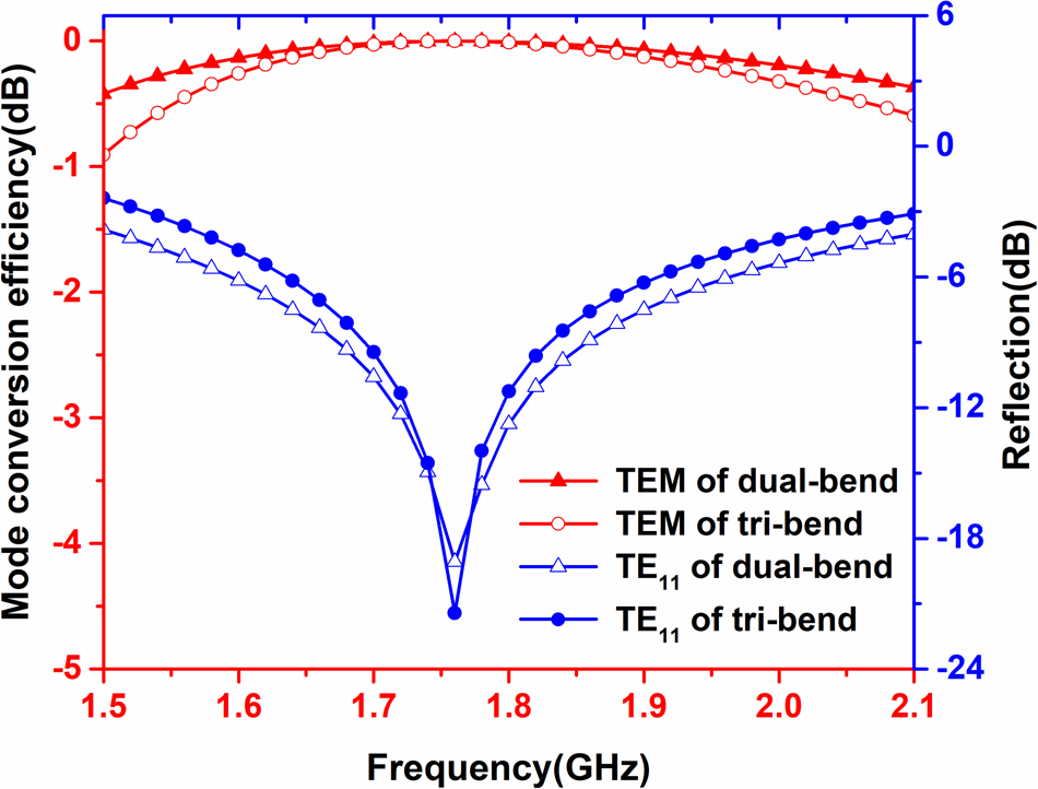
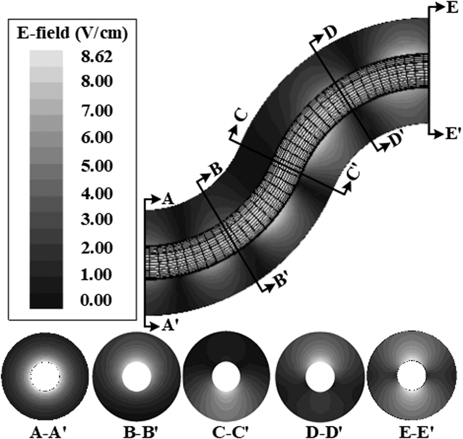
Based on the derived formulas, a dual-bend TEM-TE₁₁ mode converter at 1.75 GHz is designed. The cross-section size of the waveguide bend is predetermined with a = 60 mm and b = 20 mm to realize the cut-off of the high-order modes and meet the requirements of the L-band coaxial relativistic backward wave oscillator in our lab [Reference Ge, Zhong, Qian, Zhang, Gao, Jin, Fan and Yang16]. The maximum conversion efficiency can be achieved by taking R ₁ = –R ₂ = 182.5 mm, L = 0 mm, and θ ₁ = –θ ₂ = 66.48°. As can be seen in Fig. 5, the conversion efficiency of the designed converter is better than −0.01 dB at a central frequency of 1.75 GHz. In the range of 1.5–2.1 GHz, the conversion efficiency is better than −0.05 dB; the corresponding bandwidth is over 34.28%. Figure 6 shows the electrical field distribution inside the dual-bend mode converter. Obviously, the injected coaxial TEM mode has been transformed into coaxial TE₁₁ mode totally and no electric field concentration is found inside the mode converter. As can be seen, the maximum electric field inside the converter is 8.62 V/cm when the input power is 1 W. Generally, the converter is pumped into the high-vacuum state for HPM application, in which the electric field breakdown threshold is greater than 500 kV/cm [Reference Chang17]. Therefore, according to equation (21), we can conclude that the power-handling capacity of the converter is over 3 GW.

(21)$$P_{\max} = \left( {\displaystyle{{E_{\max}} \over {E_{input{\rm -}\max}}}} \right)^2 \times P_{input}$$

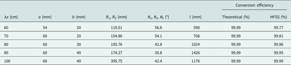
Furthermore, the length of the straight coaxial waveguide can be adjusted to realize a certain offset Δx from the axis of the output port to the axis of the input port. Based on equations (1) and (15), mode converters with different axis offsets Δx are designed and simulated. The geometric parameters and the corresponding mode conversion efficiency, as a function of Δx, are given in Table 1. As can be seen, the dual-bend mode converters can realize an over 99.5% conversion efficiency in a wide range of the axis offset Δx. The simulation results accord well with the theoretical results, which demonstrates the feasibility of the design.

Fig. 5.

Frequency responses of the dual-bend and tri-bend coaxial waveguide mode converters.

Fig. 6.

Electric field distribution of the dual-bend mode converter.

Table 1.

Geometric parameters and simulation results of the mode converter.

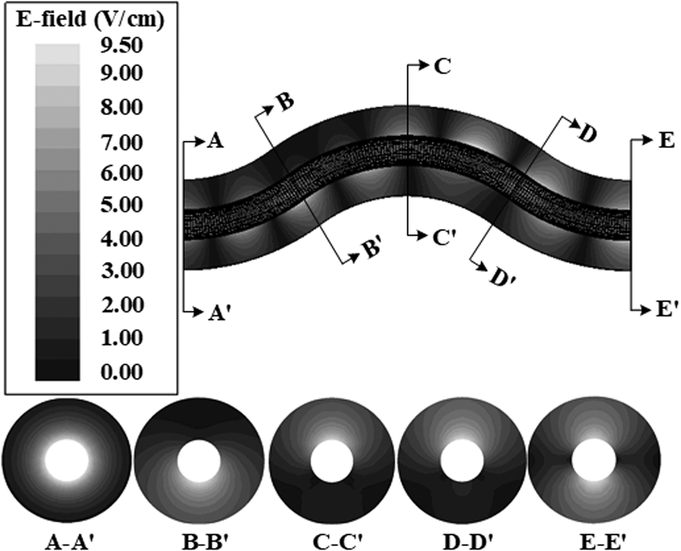
Since the input and output ports of the dual-bend mode converters are not aligned on the same axis, a tri-bend TEM to the TE₁₁ coaxial waveguide mode converter with the central frequency of 1.75 GHz is designed to overcome the shortcoming. On the basis of the theoretical analysis, the curvature radii shown in Fig. 2 are set the same, which is 258.10 mm, and the bend angles are taken as 2θ ₁ = –θ ₂ = 2θ ₃ = 72.36°. The mode conversion efficiency as a function of frequency is shown in Fig. 5, it has a high-conversion efficiency of over −0.01 dB at central frequency, and in the range of 1.56–2.06 GHz, it is better than −0.05 dB and the corresponding bandwidth is 28.57%. As shown in Fig. 7, no electric concentration is found inside the converter and the output mode is almost TE₁₁ mode. The maximum electric field inside the tri-bend converter is 9.5 V/cm with an input power of 1 W, which indicates that the power-handling capacity of the converter is over 2.5 GW.

Fig. 7.

Electric field distribution of the tri-bend mode converter.

Experiments

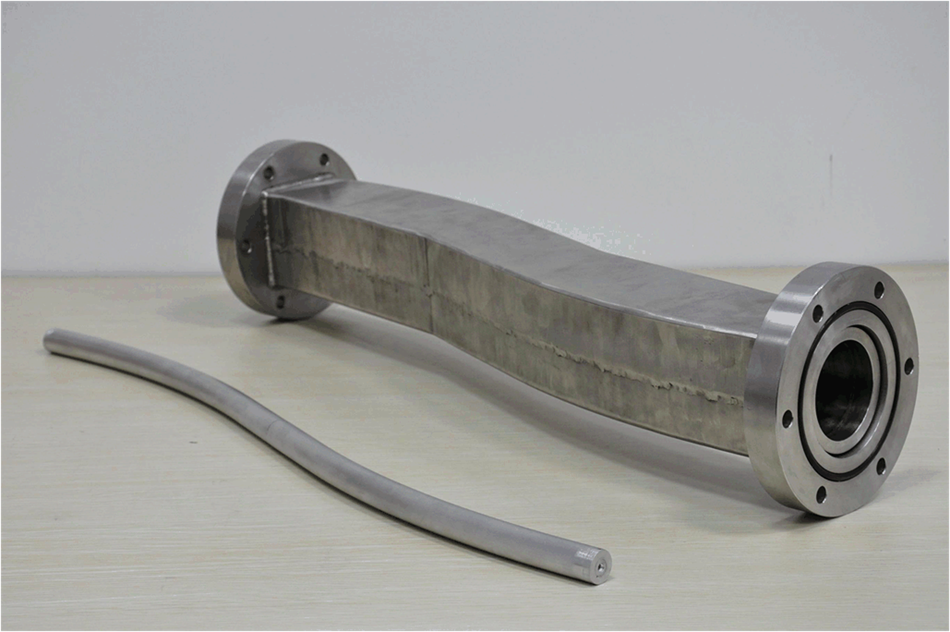
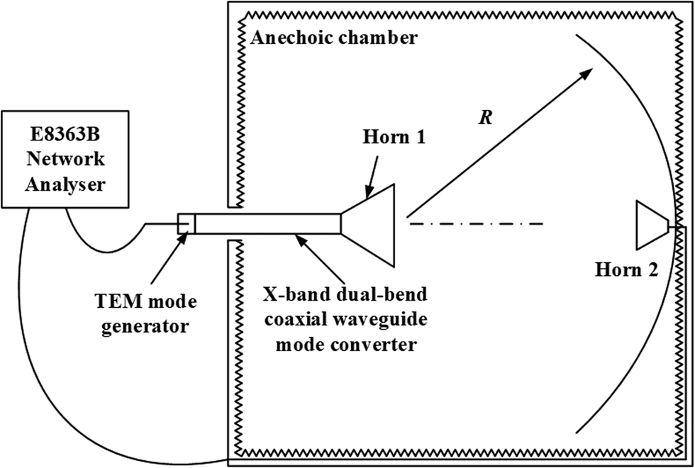
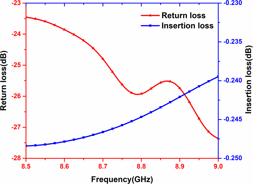
Considering the available sources in our lab and the difficulties of manufacturing and experiment operations [Reference Zhang, Ge, Zhang, He, Fan, Li, Jin, Gao, Ling and Qi18], a combined dual-bend converter shown in Fig. 8 is designed at 8.84 GHz to verify the above-mentioned analysis and design. The outer and inner diameters of the coaxial waveguide are set at 31 mm and 10 mm, separately. The maximum conversion efficiency was achieved by taking R ₁ = –R ₂ = 692.60 mm, L = 138.43 mm, and θ ₁ = –θ ₂ = 22.89°. Since it is difficult to experimentally measure the energy proportion, far field radiation patterns were used to verify the output modes and properties of the mode converter [Reference Doane19]. Figure 9 shows the layout of the cold test, which was carried out in the anechoic chamber to ensure the accuracy of the experiment. The TEM mode generator was adopted to input TEM coaxial waveguide mode into the mode converter, which was then converted into coaxial TE₁₁ mode and radiated by horn 1. By comparing the waveforms measured from the E-plane and H-plane by horn 2, the output modes of the converter could be distinguished. The distance between the receiving horn and the radiation horn is 8.5 m and the cable we use is 22 m long, with the cable loss of about 0.9 dB/m. By testing with and without the mode converter, we can easily obtain the properties of the device. As can be seen in Fig. 10, the measured reflection is lower than −23 dB in the range of 8.5–9.0 GHz, and the insertion loss is over −0.25 dB. It is concluded that the converter has a small reflection and good transmission characteristics.

Fig. 8.

Photo of the combined dual-bend TEM-TE₁₁ coaxial waveguide mode converter.

Fig. 9.

Layout of the cold test.

Fig. 10.

Return loss and insertion loss of the dual-bend mode converter.

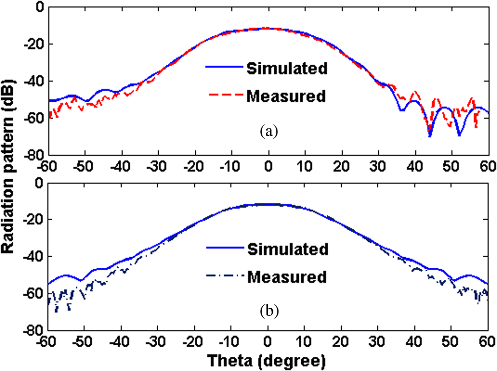
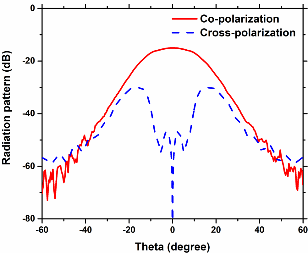
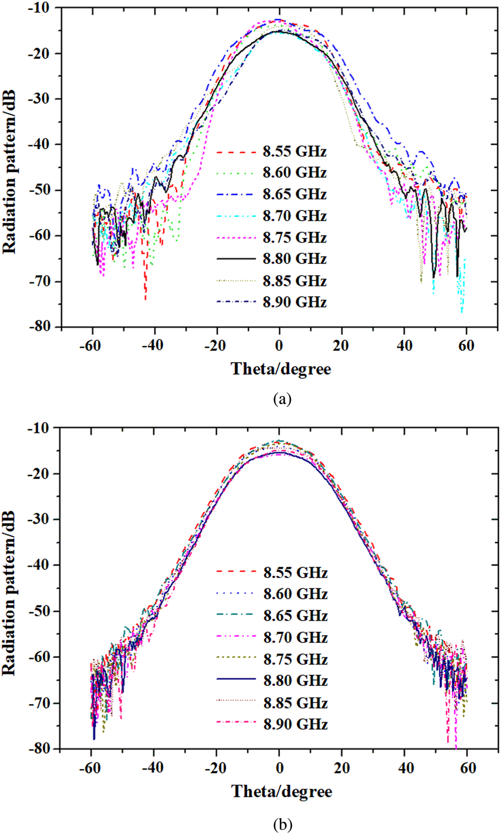
As shown in Fig. 11, the maximum radiation field appeared in the axis position, and the simulation results agreed well with the experimental results. Obviously, the radiation patterns have the characteristics of TE₁₁ mode, indicating that the main output mode is TE₁₁ mode. Figure 12 shows the comparison of the radiation patterns of co-polarization and cross-polarization. It can be concluded that the main-lobe gain of the cross-polarization is about 15 dB lower than that of the co-polarization, which demonstrates the high-conversion efficiency of the converter. Moreover, as can be seen in Fig. 13, the radiation distribution stayed almost the same within 8.55–8.95 GHz, which was the further validation of stability and bandwidth of the converter.

Fig. 11.

Measured radiation patterns: (a) E-plane and (b) H-plane.

Fig. 12.

Radiation patterns comparison of co-polarization and cross-polarization.

Fig. 13.

Radiation patterns in the range of 8.55–8.95 GHz: (a) E-plane, and(b) H-plane.