1 Introduction
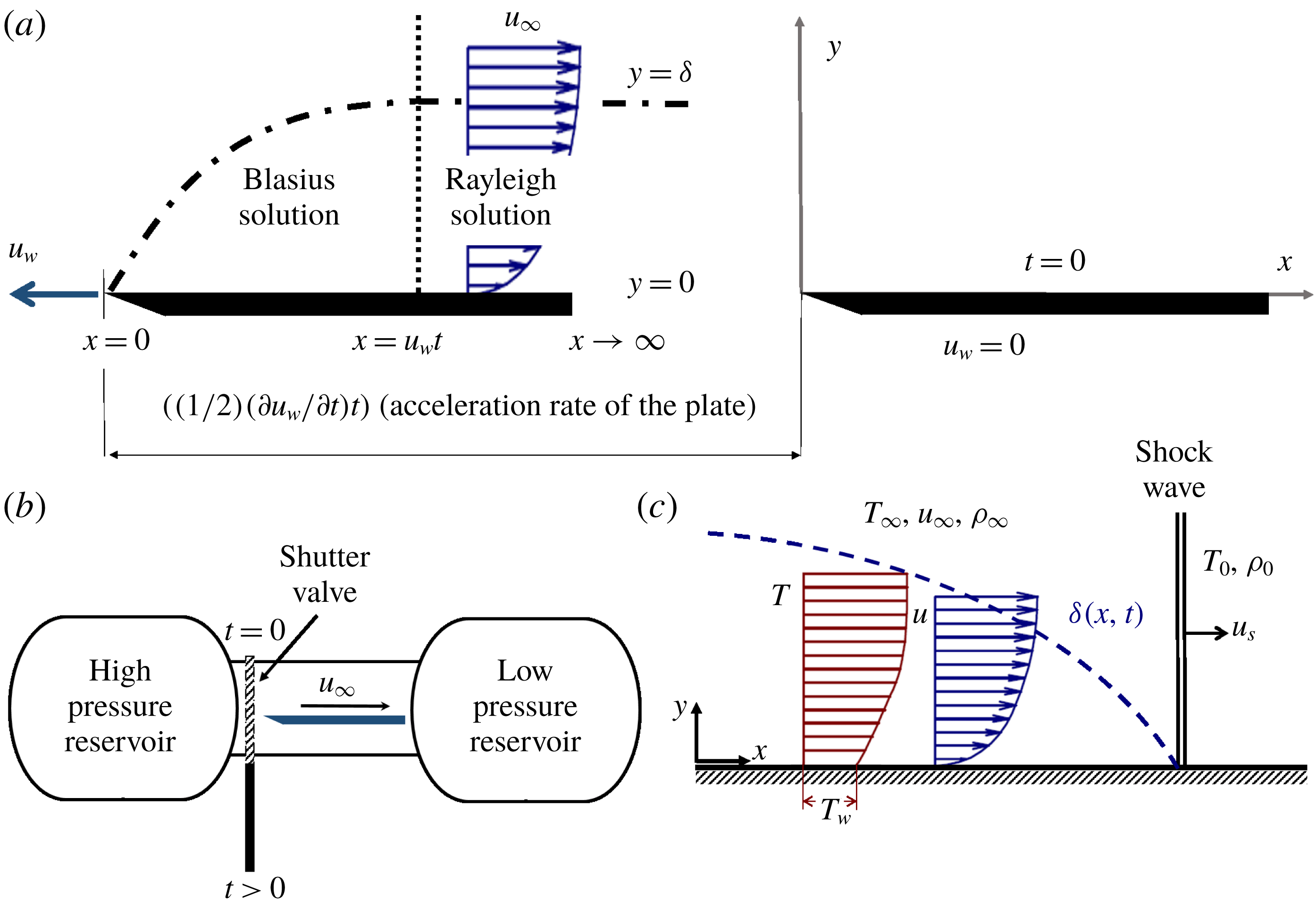
The time sequence of the laminar boundary layer initiation was previously documented in theoretical and analytical studies with various degrees of simplicity. Stewartson (Reference Stewartson1950, Reference Stewartson1960) focused on the impulsive start of motion of semi-infinite flat plates. Considering short time scales, the boundary layer over an accelerated flat plate could be divided into two regions, sketched in figure 1(a). The boundary layer is independent of the axial position for
 $u_{w}t<x$
, because the effect of the leading edge has not arrived there yet. The boundary layer in this region corresponds to a Rayleigh profile (Rayleigh Reference Rayleigh1911; Schlichting Reference Schlichting2003). In the part where
 $u_{w}t>x$
, the low momentum flow is independent of time and responds to a Blasius profile (Blasius Reference Blasius1908, Reference Blasius1950) growing from the leading edge of the plate, where
 $t$
is the time,
 $x$
is the axial distance and
 $u_{w}$
is the wall velocity. In cases of larger time scales, the entire plate is affected by the leading edge presence and the solution of the boundary layer should be expressed as a function of the axial position. Moore (Reference Moore1951) performed a dimensionless analysis of the establishment of the flow over a flat plate, set into motion with a time-dependent velocity. The time response of the laminar boundary layer (
 $\unicode[STIX]{x1D70F}_{flow\;establishment}$
) is thereby driven by the kinematic viscosity (
 $\unicode[STIX]{x1D708}$
) across the boundary layer thickness (
 $\unicode[STIX]{x1D6FF}$
):
 $$\begin{eqnarray}\unicode[STIX]{x1D70F}_{flow\;establishment}=\frac{\unicode[STIX]{x1D6FF}^{2}}{\unicode[STIX]{x1D708}}.\end{eqnarray}$$
Ostrach (Reference Ostrach1952) determined the effect of heat transfer on the formation of the aerodynamic boundary layer. A wall temperature (
 $T_{w}$
) larger than the free stream temperature (
 $T_{\infty }$
) (temperature ratio
 $TR=T_{\infty }/T_{w}$
lower than 1) leads to thinner boundary layers, consequently leading to higher skin friction coefficients, but shorter establishment processes.
Smith & Edward (Reference Smith1996) studied the starting process in a reflected shock tunnel. Their experimental work substantiated the relevance of the flow transient effects towards the characterization of the boundary layer formation. Wen-Jei & Huang-Sen (Reference Wen-Jei and Huang-Sen1968) demonstrated analytically the prime influence of the acceleration rate on the boundary layer development, derived from the skin friction coefficient and heat transfer evolution on isothermal flat plates. Based on the exact solution of the Navier–Stokes equations for two-dimensional incompressible laminar flow, Watson (Reference Watson1958) predicted that the skin friction establishment time (
 $\unicode[STIX]{x1D70F}_{c_{f}}$
) was
 $$\begin{eqnarray}\unicode[STIX]{x1D70F}_{c_{f}}=\frac{\unicode[STIX]{x1D6FF}^{\ast 2}}{\unicode[STIX]{x1D708}}\end{eqnarray}$$
while the time required by the flow to reach the steady-state regime was estimated to be three times
 $\unicode[STIX]{x1D70F}_{c_{f}}$
. Equation (1.2) predicts an establishment time which is one third of that proposed by (1.1) for laminar flow. Note that the displacement thickness (
 $\unicode[STIX]{x1D6FF}^{\ast }$
) in a laminar boundary layer can be approximated to one third of the boundary layer thickness (Schlichting Reference Schlichting2003).
Most analytical investigations available in the literature considered the case of a laminar boundary layer under quasi-steady conditions and pure molecular diffusion. Their applicability is thus constrained to the range of impulsive starts or specific unsteady evolutions, for which the second derivative of the flow speed is negligible compared to the mean stream velocity. For turbulent flows, the time required for the boundary layer to achieve the steady state should be reduced due to the increased mixing of the flow, which can be modelled as an increase in fluid viscosity. As per the authors’ knowledge, there are no published analytical studies on turbulent boundary layer inception.
(a) Boundary layer development, (b) simulated process, (c) boundary layer after the passage of a shock wave.

Heat transfer research in aerospace components is typically performed in short-duration wind tunnels because they offer large temperature gradients and hence better accuracy than continuous running facilities. In blowdown wind tunnels (figure 1
b), the flow is set into motion following a sudden valve opening, causing pressure waves to travel all along the test section. Mirels (Reference Mirels1956) analysed the boundary layer growth during the flow start up after the passage of a shock wave, as depicted in figure 1(c). Holden (Reference Holden1971) studied experimentally the establishment of detached flows in the supersonic regime, and reported that the time to reach steady state is a function of test article length (
 $L$
), the flow speed (
 $u$
), Reynolds number (
 $Re$
), Mach number (
 $M$
) and the gas-to-wall temperature ratio (
 $T_{wall}/T_{\infty }$
):
 $$\begin{eqnarray}\unicode[STIX]{x1D70F}\frac{u}{L}=f(M,Re,T_{w}/T_{\infty }).\end{eqnarray}$$
Lee & Lewis (Reference Lee and Lewis1993) performed several numerical simulations that validated Holden’s model and provided predictions of the time to develop the boundary layer over a wide range of aerodynamic shapes. Similarly, Davies & Bernstein (Reference Davies and Bernstein1969) conducted experiments in order to characterize the establishment of a shock-induced boundary layer on a semi-infinite flat plate. Using the establishment parameter defined by Holden, it was found that the heat flux attains a steady-state level after a characteristic time defined as
 $\unicode[STIX]{x1D70F}(u/L)=3.3$
.
The starting of the aerodynamic boundary layer is responsible of severe thermal transport phenomena. However, the lack of precise characterization of the thermal boundary layer inception has prevented the exploitation towards compact heat exchangers and fluid machinery operating at pulsating conditions. In this paper, we describe the evolution of the aerodynamic and thermal boundary layer through successive numerical studies, ranging from adiabatic to full conjugate evaluations. The momentum and thermal boundary layer initiation was characterized for a variety of blowdown processes in the compressible flow regime. This paper quantifies the effect of Reynolds number, temperature, plate length, acceleration rate and free stream velocity on the establishment time at several start-up conditions using unsteady Reynolds averaged Navier–Stokes simulations and inviscid Euler evaluations.
2 Methodology
2.1 Geometry and problem statement
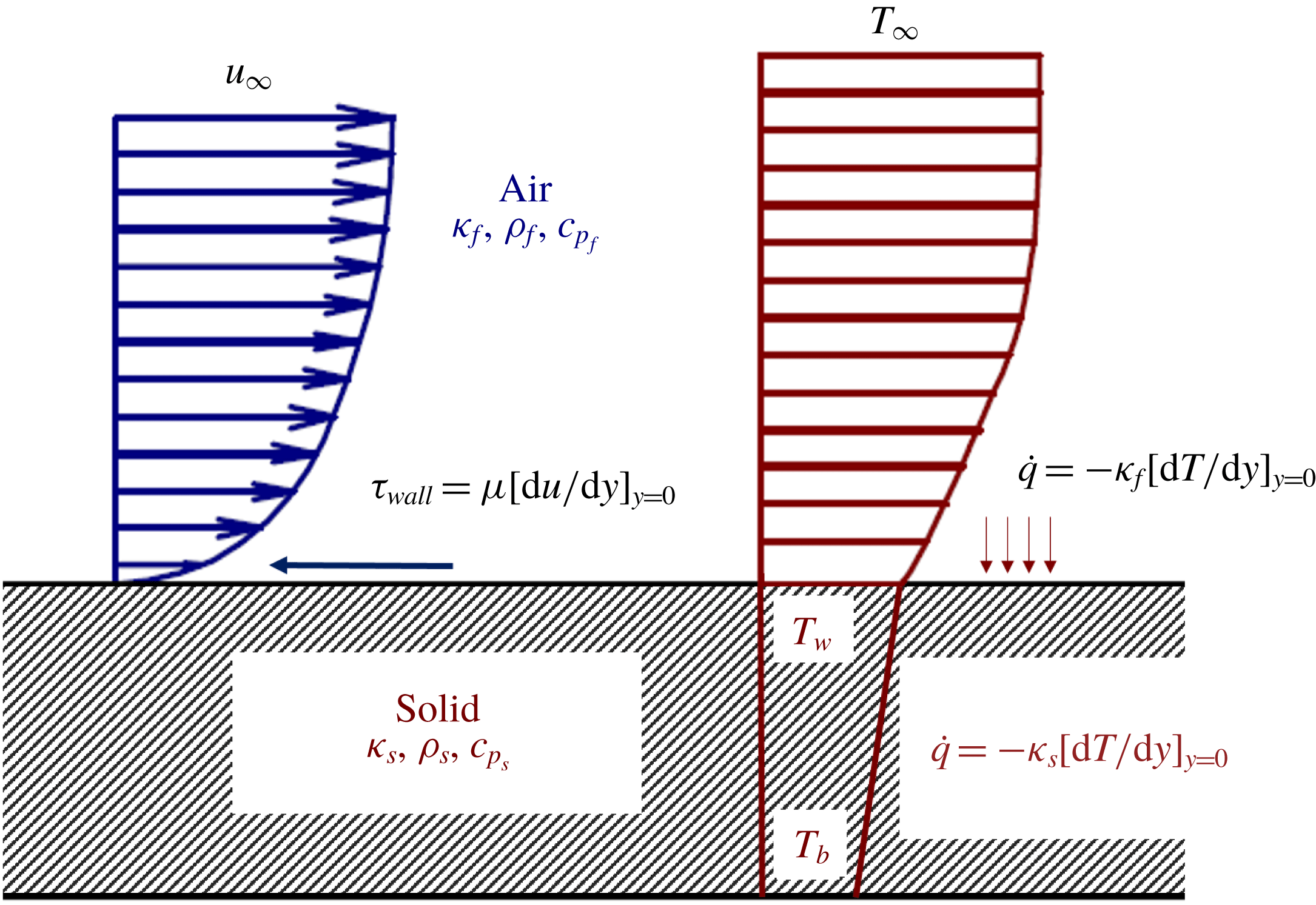
To characterize the transient response of the thermal boundary layer inception, the selected test model is a flat plate exposed to a sudden transient evolution from a no-flow to a steady-state regime, which is called a blowdown process. The objective is to quantify the temporal lag of heat transfer in a wide range of boundary conditions (adiabatic, isothermal and full conjugate). A total of 85 different blowdowns were performed changing several parameters; Reynolds number, wall temperature and pressure slope (flow acceleration). The test model consisted of a flat plate, and the simulations were performed with an unsteady Reynolds averaged Navier–Stokes (URANS) solver. In this study the flat plate was located between a high pressure reservoir and a low pressure reservoir. The thermal transient was evaluated considering the conjugate effects, as previously proposed by Perelman (Reference Perelman1961) and Luikov, Aleksashenko & Aleksashenko (Reference Luikov, Aleksashenko and Aleksashenko1971). Figure 2 represents the velocity and temperature profiles of the investigated conjugate problem, the momentum and energy equations of the fluid are coupled with the energy equation through the solid, and solved together. Following this procedure, both momentum and thermal boundary layer are resolved among with the thermal distribution across the solid. Each blowdown unsteady Reynolds-average Navier–Stokes (URANS) simulation required 8000 CPU hours in a Dell Precision Tower 7810 machine.
Flat plate momentum and thermal boundary layers under conjugate effects.

2.2 Computational domain, boundary and initial conditions
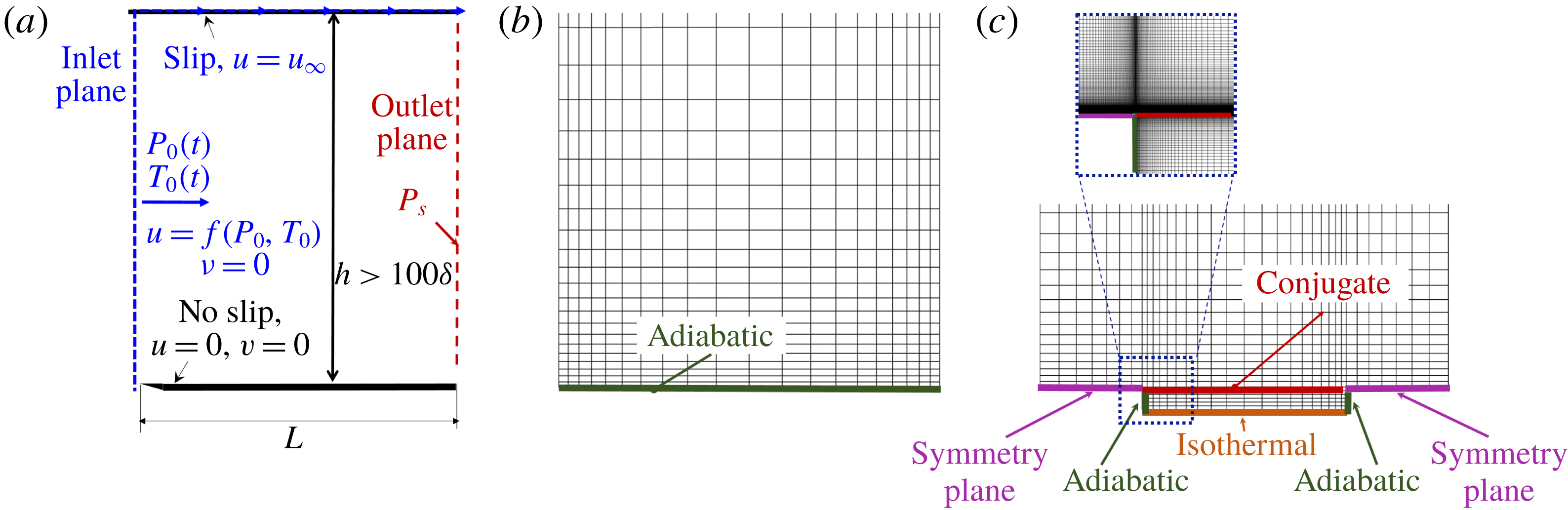
The dimensions of the computational domain displayed in figure 3 were defined to minimize the computational time. The inlet of domain is over the leading edge of the plate and the outlet just over its trailing edge, hence the plate length,
 $L$
, is also the axial dimension of the domain. The height of the domain,
 $h$
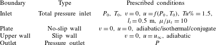
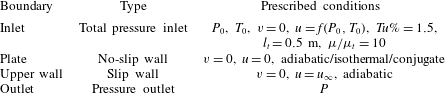
, was set to at least 100 times the boundary layer thickness. The isothermal study differs from the adiabatic calculation in the wall boundary condition, figure 3(b). For the conjugate simulations symmetry planes were used at both leading and trailing edges. Figure 3(c) shows the numerical domain including the solid region below the conjugate boundary and a zoom on the leading edge of the plate displaying the mesh resolution. For the three cases, adiabatic isothermal and conjugate, the baseline domain is a 0.5 m long flat plate. The inlet boundary condition, imposed over the normal plane of the leading edge of the plate, is a total pressure boundary condition which allows the control of the total pressure and total temperature. The turbulence intensity, length scale (
 $l_{t}$
) and viscosity ratio are imposed at the inlet to be 1.5 %, 0.5 m and 10 respectively. The inlet turbulence settings were common for all the numerical blowdowns performed on the different sections presented in the manuscript. The total inlet quantities were prescribed following the transient profiles corresponding to each case investigated. The discharge of the flow at the leading edge is perpendicular to the inlet promoting axial flow:
 $u=f(P_{0},T_{0},P,t)$
,
 $v=0$
. The outlet of the domain is modelled with a static pressure outlet, mimicking the direct discharge to a large reservoir. The static pressure level is the unique quantity fixed at the outlet and maintained at a constant level during the transient evaluation. The plate was modelled as a viscous surface, while the upper boundary of the domain was modelled using a non-reflecting slip plane. The prescribed boundary conditions are also summarized in table 1. For all of the transient evaluations the domain was initialized with zero flow velocity and a static fluid temperature equal to the prescribed wall temperature of the plate. Similarly, the static pressure level in the domain prior to the blowdown was set to the reservoir pressure imposed at the outlet. The turbulence intensity and the other turbulent parameters (turbulence intensity, length scale and turbulent viscosity ratio) were initialized to zero in all of the fluid domain.
Computational domains: (a,b) momentum boundary layer research, (c) conjugate research.

For each one of the simulations a grid sensitivity analysis was performed, following the procedure presented by Celik (Reference Celik2008). In addition, to resolve the viscous sublayer and guarantee the solver accuracy
 $y^{+}$
was kept below 0.7.
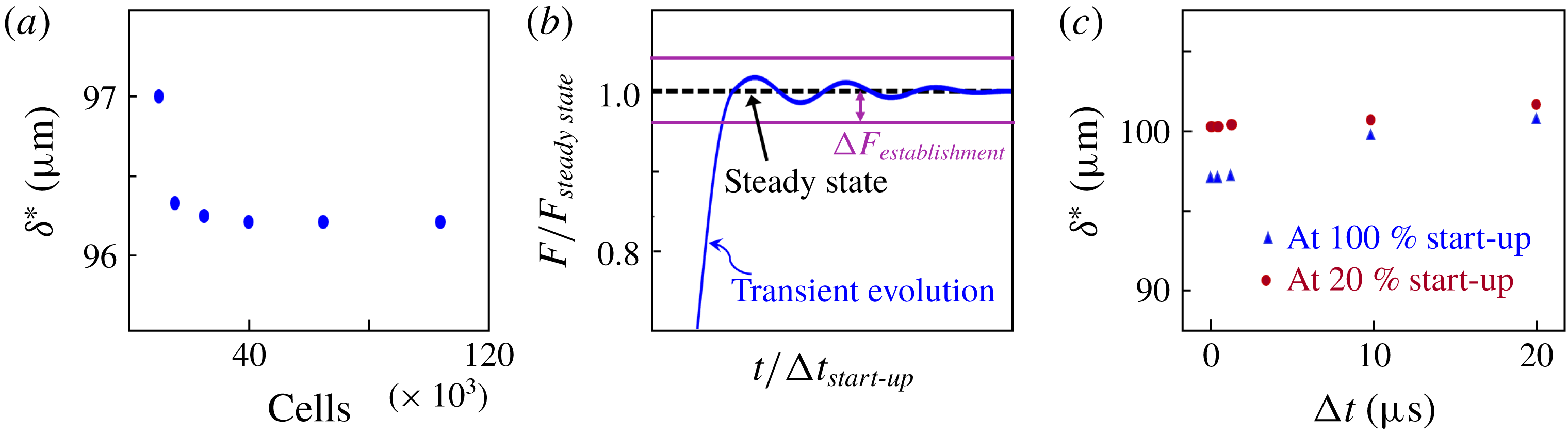
(a) Mesh sensitivity analysis, (b) establishment criteria, (c) time step benchmark analysis.

Prescribed boundary conditions.
As an example of the sensitivity analysis performed figure 4(a) represents the boundary layer displacement thickness for different mesh resolutions 100 mm downstream of the inlet for a steady state simulation at the baseline final flow conditions. An asymptotic evolution is noticed for refined meshes with more than forty thousand cells. The grid convergence index of the cited mesh was 0.71 %, therefore for this case the mesh of 40 000 was selected for the computational research, which guarantees the spatial discretization independence of the results.
2.3 Description of the computational fluid dynamics (CFD) solvers
In the present work, to assess the viscous effects on the far field flow establishment, the results were compared with simulations evaluated with a one-dimensional (1-D) Euler code. The mono-dimensional compressible real gas Euler equations implemented in this solver are expressed as:
 $$\begin{eqnarray}\frac{\unicode[STIX]{x2202}W}{\unicode[STIX]{x2202}t}+\frac{\unicode[STIX]{x2202}}{\unicode[STIX]{x2202}x}(V_{1})=0,\end{eqnarray}$$
where
 $W$
is the dependent variable vector,
 $V_{1}$
is the inviscid flux vector given as
 $$\begin{eqnarray}W=\left(\begin{array}{@{}c@{}}e\\ \unicode[STIX]{x1D70C}\\ \unicode[STIX]{x1D70C}u\end{array}\right);\quad V_{1}=\left(\begin{array}{@{}c@{}}(e+p)u\\ \unicode[STIX]{x1D70C}u\\ \unicode[STIX]{x1D70C}u^{2}+p\end{array}\right).\end{eqnarray}$$
The variable
 $e$
is the total energy,
 $\unicode[STIX]{x1D70C}$
is the density,
 $p$
is the static pressure and
 $u$
axial velocity component. This 1-D explicit Euler finite volume code was specifically developed for this application using a scheme which is second-order space and time accurate. The solver was programmed in Matlab making use of object-oriented design. To solve the inter-cell flux, a Hancock predictor corrector scheme was implemented. We used Harten-Lax–van Leer contact as our Riemann solver, taking advantage of the modified van Albada flux limiter (Kermani, Gerber & Stockie Reference Kermani, Gerber and Stockie2003). In order to impose the boundary conditions at the inlet and outlet two ghost cells were created. Then, the Riemann problem is solved between the external virtual cells and the domain cells. By using two cells on each boundary we allow the applicability of the same scheme through the entire domain enhancing the dynamic stability. Finally, the local time step for the simulation was set based on the stability criteria, in this case making use of the Courant–Friedrichs–Lewy (CFL) condition.
 $$\begin{eqnarray}0.5>\frac{(u+c)\,\text{d}t}{L}.\end{eqnarray}$$
The prescribed CFL number was strictly applied to the 1-D explicit Euler simulations which are inviscid. The URANS simulations were performed with the implicit solver CFD
 $++$
, that adopts an automatic procedure to adjust the CFL in order to reduce the time step before instabilities occur, which may affect solution. The automatic procedure will keep the CFL at lower levels during strong transients, but will allow the time step to increase again for small-amplitude flow variations. In order to apply the CFL conditioning on the viscous term and guarantee the stability of the viscous expressions, CFD
 $++$
takes advantage of the model proposed by Vigneron, Deliége & Essers (Reference Vigneron, Deliége and Essers2006) by adding an additional limit on the preconditioning parameter.
The selected 2-D URANS solver for this research is CFD
 $++$
developed by Metacomp®. The two-dimensional compressible real gas Navier–Stokes equations implemented in CFD
 $++$
are expressed as:
 $$\begin{eqnarray}\frac{\unicode[STIX]{x2202}Q}{\unicode[STIX]{x2202}t}+\frac{\unicode[STIX]{x2202}}{\unicode[STIX]{x2202}x}(F_{1}+G_{1})+\frac{\unicode[STIX]{x2202}}{\unicode[STIX]{x2202}y}(F_{2}+G_{2})=0,\end{eqnarray}$$
where
 $Q$
is the dependent variable vector,
 $F_{1}$
and
 $F_{2}$
are the inviscid flux vectors and
 $G_{1}$
and
 $G_{2}$
are the viscous flux vectors, given as
 $$\begin{eqnarray}Q=\left(\begin{array}{@{}c@{}}e\\ \unicode[STIX]{x1D70C}\\ \unicode[STIX]{x1D70C}u\\ \unicode[STIX]{x1D70C}v\end{array}\right);\quad F_{1}=\left(\begin{array}{@{}c@{}}(e+p)u\\ \unicode[STIX]{x1D70C}u\\ \unicode[STIX]{x1D70C}u^{2}+p\\ \unicode[STIX]{x1D70C}uv\end{array}\right);\quad F_{2}=\left(\begin{array}{@{}c@{}}(e+p)v\\ \unicode[STIX]{x1D70C}v\\ \unicode[STIX]{x1D70C}uv\\ \unicode[STIX]{x1D70C}uv^{2}+p\end{array}\right)\end{eqnarray}$$
 $$\begin{eqnarray}G_{1}=\left(\begin{array}{@{}c@{}}\dot{q}_{x}-u\unicode[STIX]{x1D70F}_{xx}-v\unicode[STIX]{x1D70F}_{xy}\\ 0\\ -\unicode[STIX]{x1D70F}_{xx}\\ \unicode[STIX]{x1D70F}_{xy}\end{array}\right);\quad G_{2}=\left(\begin{array}{@{}c@{}}\dot{q}_{y}-u\unicode[STIX]{x1D70F}_{yx}-v\unicode[STIX]{x1D70F}_{yy}\\ 0\\ -\unicode[STIX]{x1D70F}_{yx}\\ \unicode[STIX]{x1D70F}_{yy}\end{array}\right),\end{eqnarray}$$
where
 $v$
represents the normal velocity component,
 $\unicode[STIX]{x1D70F}$
represents the shear stress and
 $\dot{q}$
the heat flux. The shear stresses are linearly related by:
 $$\begin{eqnarray}\unicode[STIX]{x1D70F}_{xx}=2\unicode[STIX]{x1D707}\frac{\unicode[STIX]{x2202}u}{\unicode[STIX]{x2202}x}-2/3\unicode[STIX]{x1D707}\unicode[STIX]{x1D719};\quad \unicode[STIX]{x1D70F}_{yy}=2\unicode[STIX]{x1D707}\frac{\unicode[STIX]{x2202}v}{\unicode[STIX]{x2202}y}-2/3\unicode[STIX]{x1D707}\unicode[STIX]{x1D719};\quad \unicode[STIX]{x1D70F}_{xy}=\unicode[STIX]{x1D70F}_{xy}=2\unicode[STIX]{x1D707}\left(\frac{\unicode[STIX]{x2202}u}{\unicode[STIX]{x2202}y}+\frac{\unicode[STIX]{x2202}v}{\unicode[STIX]{x2202}x}\right)\!.\end{eqnarray}$$
With
 $\unicode[STIX]{x1D707}$
the coefficient of viscosity and
 $\unicode[STIX]{x1D6F7}$
the dilatation
 $$\begin{eqnarray}\unicode[STIX]{x1D6F7}=\frac{\unicode[STIX]{x2202}u}{\unicode[STIX]{x2202}x}+\frac{\unicode[STIX]{x2202}v}{\unicode[STIX]{x2202}y}.\end{eqnarray}$$
While the heat fluxes are evaluated following Fourier’s law of conduction, with
 $\unicode[STIX]{x1D705}$
the thermal conductivity of the fluid
 $$\begin{eqnarray}\dot{q}_{x}=-\unicode[STIX]{x1D705}\frac{\unicode[STIX]{x2202}T}{\unicode[STIX]{x2202}x};\quad \dot{q}_{y}=-\unicode[STIX]{x1D705}\frac{\unicode[STIX]{x2202}T}{\unicode[STIX]{x2202}y}.\end{eqnarray}$$
In this solver the fluid flow equations are discretized in the spatial domain using the cell centred finite volume approach. The inviscid flux function is a second-order, upwind scheme using a Harten-Lax–van Leer contact Riemann solver and a multi-dimensional minmod flux limiter (Roe Reference Roe1986), while centroidal-based out-of-face polynomials were used for the viscous fluxes. The governing equations of the flow were solved with a perfect gas density-based algorithm. Additionally, the first-/second-order blending technique was used to accelerate convergence. In order to reduce the computational burden, a multi-grid technique with four levels was utilized. The turbulence closure was achieved with the
 $\unicode[STIX]{x1D705}{-}\unicode[STIX]{x1D714}$
shear stress transport turbulence model, (Menter Reference Menter1994). The
 $\unicode[STIX]{x1D705}{-}\unicode[STIX]{x1D714}$
shear stress transport (SST) turbulence model consists of a blending approach between the
 $\unicode[STIX]{x1D705}{-}\unicode[STIX]{x1D714}$
model in the near wall region and the
 $\unicode[STIX]{x1D705}{-}\unicode[STIX]{x1D716}$
model in the free stream flow. The molecular viscosity (
 $\unicode[STIX]{x1D707}$
) variation with temperature was modelled with the Sutherland law equation (2.10). The thermal conductivity (
 $\unicode[STIX]{x1D705}$
) was modelled using the correlation proposed by Stephan & Laesecke (Reference Stephan and Laesecke1985), equation (2.11). The heat capacity dependence on the temperature was also taken into account with an eighth-order polynomial, equation (2.12). Along this line, the molecular Prandtl number variations at low temperature were considered,
 $Pr=\unicode[STIX]{x1D707}C_{p}/\unicode[STIX]{x1D705}$
. The laminar Prandtl number of the baseline case was set to
 $Pr=0.718$
.
 $$\begin{eqnarray}\left.\begin{array}{@{}c@{}}\unicode[STIX]{x1D707}=\unicode[STIX]{x1D707}_{ref}\left({\displaystyle \frac{T}{T_{ref}}}\right)^{3/2}{\displaystyle \frac{T_{ref}+S}{T+S}};\quad \unicode[STIX]{x1D707}_{ref}=1.765\text{e}^{-5}~(\text{kg}~\text{ms}^{-1});\\ T_{ref}=273.11~(\text{K});\quad S=110.4~(\text{K});\end{array}\right\}\end{eqnarray}$$
 $$\begin{eqnarray}\displaystyle \unicode[STIX]{x1D705} & = & \displaystyle (\!33.9729025\ast (T/132.52)^{-1}-164.702679\ast (T/132.52)^{-2/3}\nonumber\\ \displaystyle & & \displaystyle +\,262.108546\ast (T/132.52)^{-1/3}-21.5346955\ast (T/132.52)^{0}\nonumber\\ \displaystyle & & \displaystyle -\,443.455815\ast (T/132.52)^{1/3}+607.339582\ast (T/132.52)^{2/3}\nonumber\\ \displaystyle & & \displaystyle -\,368.790121\ast (T/132.52)^{(1)}+111.296674\ast (T/132.52)^{4/3}\nonumber\\ \displaystyle & & \displaystyle -\,13.4122465\ast (T/132.52)^{5/3} )\times 4.358\times 10^{-3}~(\text{W}~\text{mK}^{-1});\end{eqnarray}$$
 $$\begin{eqnarray}\displaystyle C_{p} & = & \displaystyle 1000\times (0.992313+(0.236688T)/1000-1.852148\ast (T/1000)^{2}\nonumber\\ \displaystyle & & \displaystyle +\,6.083152\ast (T/1000)^{3}-8.893933\ast (T/1000)^{4}+7.097112\ast (T/1000)^{5}\nonumber\\ \displaystyle & & \displaystyle -\,3.234725\ast (T/1000)^{6}+0.794571\ast (T/1000)^{7}-0.081873\ast (T/1000)^{8} )\nonumber\\ \displaystyle & & \displaystyle (\text{J}~\text{K}^{-1}).\end{eqnarray}$$
The temporal discretization scheme is a point implicit time integration, which is characterized with a local time stepping technique, defined by the CFL number. CFD
 $++$
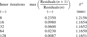
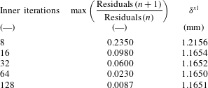
allows an automatic CFL adjustment procedure when a time step is too large in order to avoid numerical instabilities and solution divergence. In transient simulations, the solver enables the dual time stepping approach that reduces the number of internal iterations required to reach convergence in each of the time steps. The local time step was selected to provide the maximum temporal resolution to resolve transients with the lowest computational time and with sufficient frequency resolution. A benchmark analysis of the number of inner iterations was performed to ensure continuity in mass, momentum and energy. The objective of this analysis was to determine the minimum number of iterations required to guarantee the convergence of the solution through the time steps in order to reduce the computation effort. The start-up time and flow conditions were kept constant at the baseline conditions and several numerical blowdowns were modelled with different inner time steps. Considering 8–128 inner iterations, we monitored the decay in momentum, energy and turbulence parameter residuals and the change of boundary layer thickness. Table 2 presents the average of the residual decay, and displacement thickness (
 $\unicode[STIX]{x1D6FF}^{x1}$
) at
 $x=0.05~\text{m}$
and at half of the total pressure rise (
 $t=1/2\unicode[STIX]{x0394}P_{0}$
) recorded during the transient process. The displayed residual is the one that depicts the maximum ratio among those being tracked, where
 $n$
represents a given time step and
 $n+1$
the consecutive one. The only parameter changed among the different cases were the total number of inner iterations. The range of Mach and Reynolds numbers explored in this analysis ranges from 0.04 up to 0.6 and from
 $5\times 10^{5}$
up to
 $1\times 10^{7}$
respectively.
Beyond 16 iterations, the decay of the residuals was always at least by one order of magnitude. Further increase of the number of inner iterations did not improve significantly the prediction of the boundary layer height, and brought only a relatively small reduction of the residuals. Hence, the number of inner iterations was selected to be 16, which provides at least one order of magnitude of decay in the inner iteration residuals. Both solvers are assessed in the subsequent section. Additionally, the comparison of the unsteady evolution for the inviscid code and the CFD
 $++$
data provides a verification of the transient solution of the URANS tool.
Inner iteration benchmark analysis based on
 $\unicode[STIX]{x1D6FF}^{x1}$
, where
 $\unicode[STIX]{x1D6FF}^{x1}$
stands for the boundary layer height at
 $x=0.05~\text{m}$
and
 $t=1/2\unicode[STIX]{x0394}P_{0}$
.
2.4 Determination of the establishment time
Each of the transient evolutions was compared with the steady-state results. The establishment time for every quantity was determined according to the closeness to the steady-state value and the slope of its oscillation, as sketched in figure 4(b). The abscissa represents the time step over the rise time of the total pressure determining the start-up time of the inlet flow conditions,
 $\unicode[STIX]{x0394}t_{start\text{-}up}$
. Once the distance to the steady-state value of the given quantity was below its defined threshold and its oscillation was within half of that fringe, the quantity was assumed established. The thresholds
 $\unicode[STIX]{x0394}F_{establishment}$
of the wall shear stress and the heat transfer are determined based on a sensitivity analysis. In order to determine the
 $\unicode[STIX]{x0394}F_{establishment}$
multiple URANS evaluations were performed with different static-to-total pressure ratios. The total-to-static pressure level variation drives the flow acceleration, setting the flow velocity across the domain. Three different simulations were performed in this analysis, a baseline case with a total-to-static pressure difference of 10 kPa, and 2 cases with
 $+5\,\%$
and
 $-5\,\%$
variations on the total-to-static pressure difference, respectively. By comparing the results of the increased and decreased pressure ratios with the baseline case the effect of a given total-to-static pressure ratio change on the wall fluxes was retrieved. Following this procedure we could recognize the magnitude of the variations induced in the wall fluxes by a deviation of the total-to-static pressure difference. In conclusion, we selected the establishment thresholds for the wall shear stress, heat flux and axial flow velocity as the ones associated with a change in 0.5 % in the total-to-static pressure difference.
The establishment time was evaluated at three locations, leading edge, mid-chord and trailing edge of the flat plate. The trends and conclusions are independent of the considered location. To minimize the computational burden while guaranteeing the accuracy of the results, a benchmark analysis for the local time step,
 $\unicode[STIX]{x0394}t$
was carried out. Figure 4(c) represents the displacement thickness for different time steps at mid-chord. Two different flow times are depicted: at 20 % of the total pressure evolution and at the end of total pressure rise. For time steps larger than
 $10~\unicode[STIX]{x03BC}\text{s}$
there exists more than 1 % of variation with respect to the shortest time step simulation at
 $0.1~\unicode[STIX]{x03BC}\text{s}$
. We selected a time step of
 $1~\unicode[STIX]{x03BC}\text{s}$
, for which the difference compared to the results at
 $0.1~\unicode[STIX]{x03BC}\text{s}$
are below 0.05 %. The data are stored only every 10–20 physical time steps due to storage limitations, which results in a stored temporal discretization of approximately 2 % of the establishment time for the baseline case. Given the temporal resolution and the establishment determination procedure, the uncertainty in the relative establishment time is
 $\pm 0.06~\text{ms}$
.
2.5 Solver verification
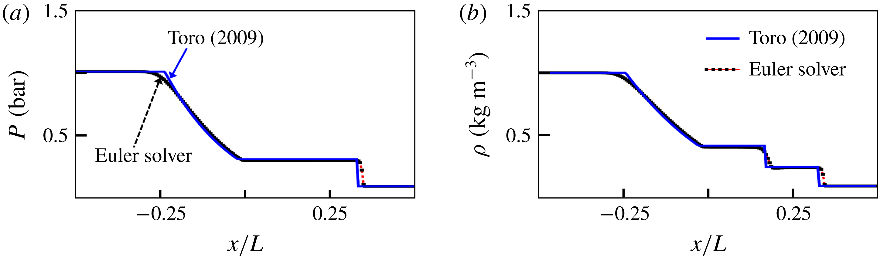
The ad hoc 1-D Euler solver was validated against the sod-shock tube problem presented by Toro (Reference Toro2009). Figure 5(a,b) displays the instantaneous pressure and density variation along the axis of a shock tube. Two zones of uniform cross-section at different pressures and temperatures are initially separated by a thin diaphragm. Following the burst of the diaphragm a normal shock travels along the driven region of the shock tube (at lower pressure) and an expansion fan travels to the driver part of the tube. After 0.2 s the diaphragm rupture the shock wave is located at
 $x/L=0.35$
. Between
 $x/L=-0.2$
and
 $x/L=0$
a gradual variation in density is induced by the expansion waves generated at the interface. At
 $x/L=0.15$
we observe the slip line or contact discontinuity between the initially compressed flow and low pressure region, moving at the flow velocity. In general, the 1-D Euler solver data, obtained with 100 cells, agrees well with the analytical solution.
Sod-shock tube Euler solver validation: (a) pressure and (b) density.

Assessment of the URANS solver (CFD
 $++$
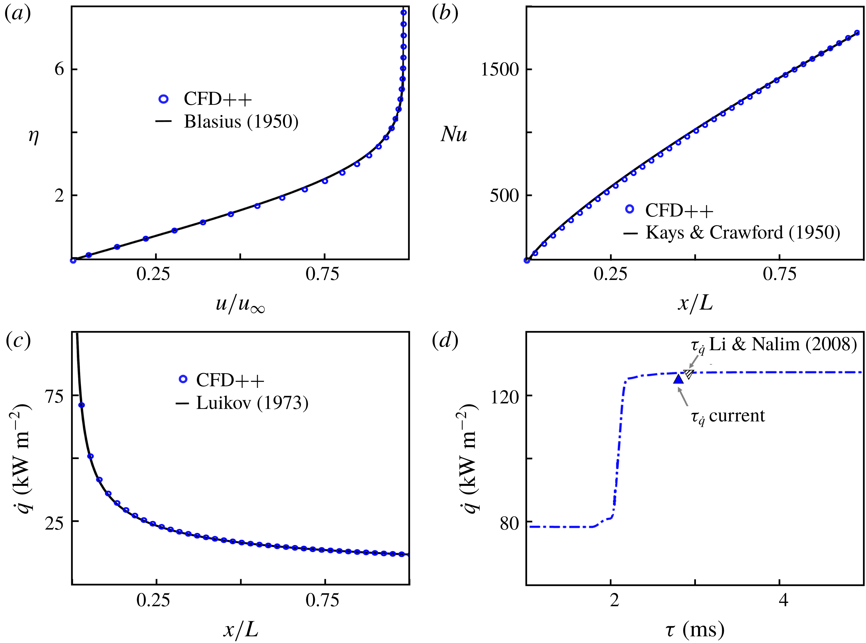
). (a) Verification of laminar flow resolution: laminar boundary layer profile, (b) verification of turbulent flow modelling: Nusselt distribution, (c) verification of conjugate module: heat transfer between solid wall and fluid flow, (d) verification of transient flow prediction: thermal boundary layer response to a sudden step in flow temperature.

Several verification tests were performed using an identical computational domain to assess the validity of the URANS solver. The purpose of this analysis was to verify the performance of our numerical set-up modelling the phenomena under study in this research, including: the laminar and turbulent aero-thermal boundary layer for isothermal and conjugate boundary conditions under unsteady mean flow conditions. Figure 6(a) shows an excellent agreement between the URANS prediction (CFD
 $++$
) of a laminar boundary layer profile compared with the Blasius profile (Blasius Reference Blasius1950), which demonstrates the ability of the solver to model the laminar boundary layer region, the difference is less than 0.1 %. The numerical domain for this case was the baseline flat plate of 0.5 m with a free stream velocity of
 $10~\text{m}~\text{s}^{-1}$
and a free stream temperature of 300 K. Regarding the assessment of the turbulent boundary layer, figure 6(b) presents the Nusselt number distribution along a flat plate from CFD
 $++$
versus the Reynolds number analogy ((2.13) Kays & Crawford (Reference Kays and Crawford1980)) with a differences of less than 0.25 %. The conjugate solver capabilities were verified by comparing the result of the conjugate problem described by Luikov (Reference Luikov1973) and Dorfman (Reference Dorfman2009). In this case the maximum difference in heat flux between the CFD
 $++$
calculations and the results presented by Luikov is 0.6 %, as depicted in figure 6(c), which illustrates a good agreement between the solver and the analytical solution for the heat flux distribution along the flat plate. For both analyses, isothermal and conjugate the numerical plate had a length of 0.5 m and the flow conditions where equivalent to the final condition of the baseline blowdown,
 $P_{0}=0.192~\text{bar}$
,
 $T_{0}=260~\text{K}$
and free stream velocity of
 $U_{\infty }=117~\text{m}~\text{s}^{-1}$
. The heat flux and derived Nusselt number were recorded along the plate upper surface upon convergence of the steady-state simulations.
 $$\begin{eqnarray}Nu=0.332Re^{-1/2}Pr^{1/3},5\times 10^{5}<Re<2\times 10^{7}.\end{eqnarray}$$
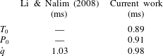
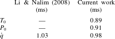
The unsteady analysis of Li & Nalim (Reference Li and Nalim2008) was used to assess the transient capability of our solver in predicting the establishment. For this verification analysis, the numerical domain was the baseline isothermal plate of 0.5 m. Figure 6(d) and table 3 depict the results obtained for a sudden thermal jump at
 $Re_{x,t=0}=1.15\times 10^{7}$
,
 $u_{\infty ,t=0}=145~\text{m}~\text{s}^{-1}$
,
 $T_{t=0}=406~\text{K}$
,
 $T_{t>t^{c}}=480~\text{K}$
,
 $\unicode[STIX]{x0394}P_{0}=19\,200~\text{Pa}$
, compared to the published data of Li & Nalim (Reference Li and Nalim2008). In this case the total temperature is increased at the bursting time
 $t^{c}$
. The results show that our solver predicts accurately the heat transfer problem, the deviation is approximately
 $50~\unicode[STIX]{x03BC}\text{s}$
.
Thermal boundary layer response to a
 $T_{0\infty }$
step.
3 Momentum boundary layer establishment
3.1 Establishment sequence
The first quantity to be established is the main flow total pressure,
 $P_{0}$
, followed by the free stream velocity,
 $u_{\infty }$
. The establishment of the total pressure and the free stream velocity is determined by the propagation of compression and expansion waves across the domain. Due to the transient inlet boundary conditions, which reflects the subsonic blowdown process, compression waves are generated at the leading edge. Then they are propagated through the domain until the outlet boundary condition is reached. At the outlet, the pressure waves face a constant pressure boundary condition, being consequently reflected as expansion waves (Lighthill Reference Lighthill2001). The establishment of the total pressure (
 $P_{0}$
) will be determined by the passage of the last compression wave, while the establishment of the free stream velocity will be set by the passage of the last expansion wave.
Once the free stream conditions are established the information needs to be propagated towards the wall across the boundary layer thickness
 $\unicode[STIX]{x1D6FF}$
, which is mainly a diffusive process. To characterize the momentum boundary layer establishment, the wall shear stress
 $\unicode[STIX]{x1D70F}_{wall}$
was used:
 $$\begin{eqnarray}\unicode[STIX]{x1D70F}_{wall}=\unicode[STIX]{x1D707}\frac{\unicode[STIX]{x2202}u}{\unicode[STIX]{x2202}y}.\end{eqnarray}$$
The establishment time of the boundary layer (
 $\unicode[STIX]{x1D70F}_{\unicode[STIX]{x1D70F}_{w}}$
), can be divided into two terms, the time to establish the free stream boundary condition and the flow total pressure (
 $\unicode[STIX]{x1D70F}_{P_{0}}$
), and then a referenced establishment time (
 $\unicode[STIX]{x1D70F}^{\ast }$
). In such expressions the subscript
 $x$
refers to the axial position where the establishment time is evaluated.
 $$\begin{eqnarray}\unicode[STIX]{x1D70F}_{x}^{\ast }=\unicode[STIX]{x1D70F}_{x}-\unicode[STIX]{x1D70F}_{P_{0}}.\end{eqnarray}$$
The independent parameters that were selected to analyse the effect on the boundary layer establishment are: free stream velocity (
 $u_{\infty }$
), global slope of transient (
 $\unicode[STIX]{x0394}P_{0}/\unicode[STIX]{x0394}t$
), free stream total temperature (
 $T_{0,\infty }$
), Reynolds number (
 $Re$
) and the length of the domain (
 $L$
).
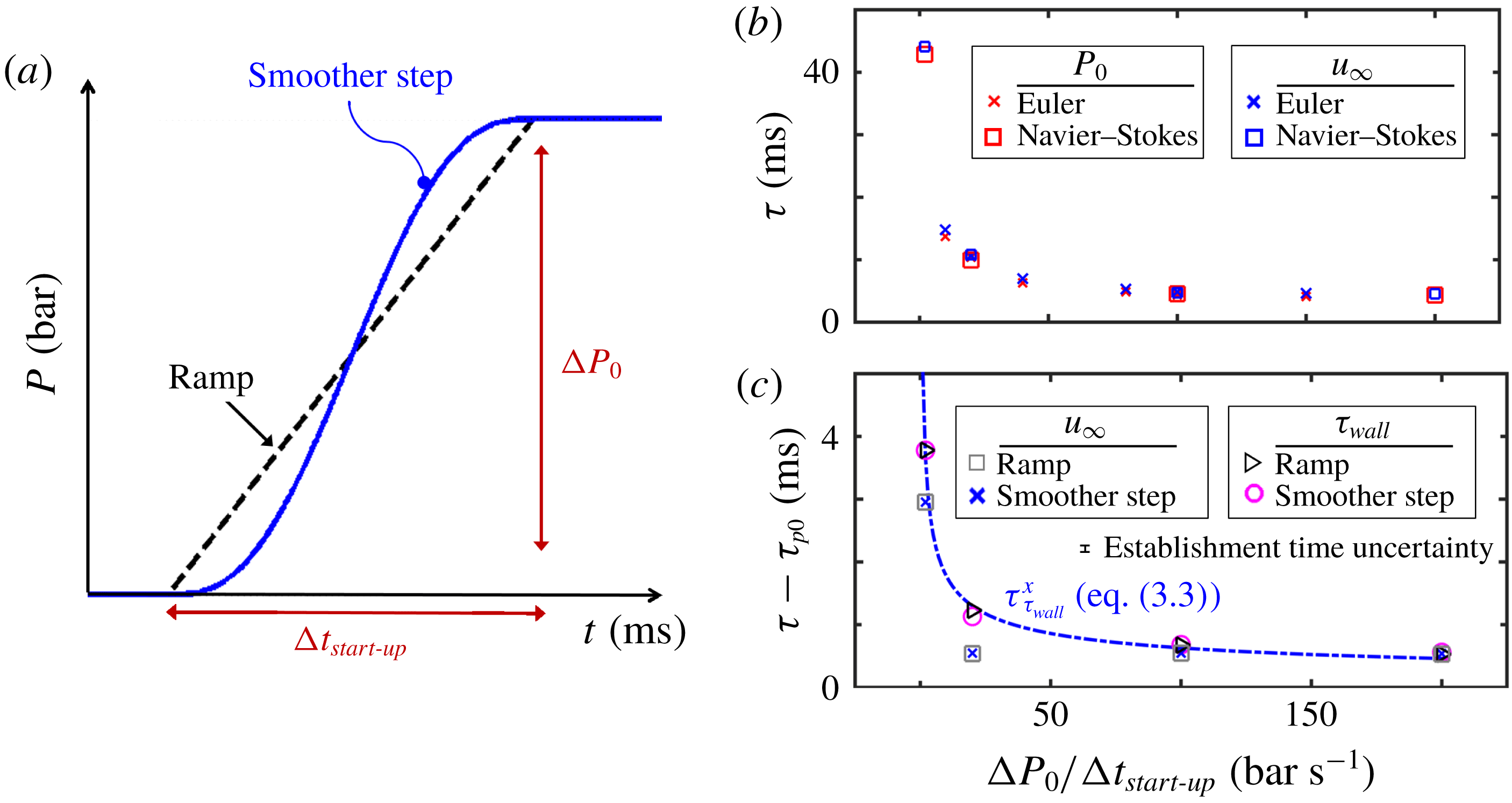
Slope effect: (a) investigated evolutions: smooth and ramp; (b) acceleration rate effect on total pressure establishment (
 $\unicode[STIX]{x1D70F}_{P_{0}}$
) and free stream velocity establishment (
 $\unicode[STIX]{x1D70F}_{u_{\infty }}$
) viscous versus inviscid; (c) flow acceleration rate effect on
 $\unicode[STIX]{x1D70F}_{u_{\infty }}^{\ast }$
(referenced free stream velocity establishment) and
 $\unicode[STIX]{x1D70F}_{\unicode[STIX]{x1D70F}_{wall}}^{\ast }$
(referenced momentum boundary layer establishment) smother step versus ramp.

3.2 Effect of the flow acceleration rate
The effect of the acceleration rate is investigated by imposing different total pressure temporal rises at the inlet of the domain. The slope of the pressure rise (
 $\unicode[STIX]{x0394}P_{0}/\unicode[STIX]{x0394}t_{start\text{-}up}$
) was evaluated for a ramp and a for smoother step. Both evolutions are displayed in figure 7(a), where smooth and sharp transitions between phases are considered. The effect of the rate of pressure rise was investigated at identical final steady flow conditions. In this study the flat plate length is 0.5 m. For the different flow acceleration rates analysed in this section the following properties were kept constant:
(i) final steady-state total pressure,
 $P_{0}=0.192~\text{bar}$
;
(ii) mean flow velocity,
$U_{\infty }=117~\text{m}~\text{s}^{-1}$
;(iii) gas total temperature,
$T_{0}=260~\text{K}$
;(iv) Reynolds number (at
$x=0.5~\text{m}$
),
$1\times 10^{6}$
.




The start-up time was varied, resulting in six different cases simulated in CFD
 $++$
, while seven cases were modelled with the inviscid solver. Figure 7(b) reports the establishment time of the total pressure and free stream velocity for a variety of start-up phase durations. The establishment of the free stream velocity drives the settlement of the flow conditions at the edge of the boundary layer. In this figure, the results of the URANS solver compare well with the ad hoc Euler numerical tool, which implies that the establishment of the total pressure and the free stream velocity is independent of the flow viscosity. Figure 7(c) depicts the referenced establishment time for the free stream velocity and the wall shear stress for a range of total pressure slopes, including smoother steps and ramp evolutions. Up to approximately
 $100~\text{bar}~\text{s}^{-1}$
there exists a clear tendency: the shorter the start-up phase duration the shorter the flow establishment time becomes. This phenomenon is driven by the stronger acceleration of the flow along the plate.
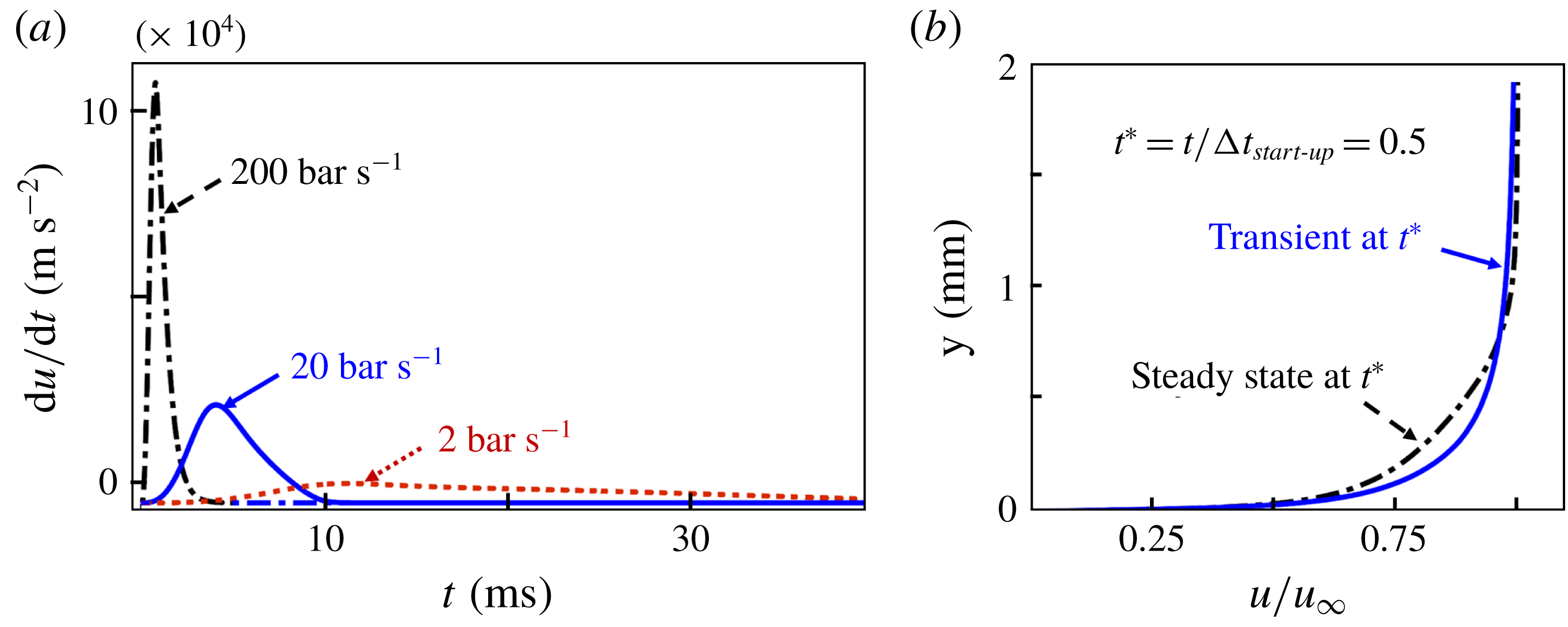
Figure 8(a) reports the core flow acceleration rate for three different blowdowns, varying the pressure increase in time. The presented acceleration rates were recorded at the half location of the plate (
 $x=0.25~\text{m}$
), at
 $y=10\unicode[STIX]{x1D6FF}^{\ast }$
. The numerical predictions show that faster pressure escalations result in a stronger initial flow acceleration rate. At higher acceleration rates, most of the compression waves are transmitted at the beginning of the process, resulting in a faster propagation of the pressure waves through the domain. Consequently, the total pressure field is established earlier.
(a) Acceleration inside of the domain; (b) steady boundary layer versus transient boundary layer at half of the start-up phase.

Figure 8(b) represents two different boundary layer profiles at half of the
 $20~\text{bar}~\text{s}^{-1}$
pressure slope blowdown simulation, at
 $x=0.05~\text{m}$
. The steady boundary layer profile is obtained at the same axial location based on a steady-state simulation run with mean flow conditions extracted from the transient calculation at the time when the total pressure rise reach half of its final value. (
 $P_{0}-P=0.096~\text{bar}$
, free stream temperature of 260 K, flow speed of
 $83.4~\text{m}~\text{s}^{-1}$
). Both boundary layers are submitted to the same free stream conditions but the accelerated boundary layer is characterized by a smaller thickness and a clear stretching. The reduction in the establishment time of the wall shear stress with faster transients (shown in figure 7
c) can be justified by the stretching of the boundary layer. Through a power law least squares fitting we found that the effect of the start-up pressure rise slope on the boundary layer establishment follows the trend:
 $$\begin{eqnarray}\unicode[STIX]{x1D70F}_{\unicode[STIX]{x1D70F}_{wall}}^{\ast }\propto \frac{1}{\sqrt{\unicode[STIX]{x0394}P_{0}/\unicode[STIX]{x0394}t_{start\text{-}up}}}.\end{eqnarray}$$
3.3 Free stream velocity
In order to decouple the effect of the Reynolds number from the convective effects, the study was carried out at the same final steady total temperature while maintaining the Reynolds number constant at
 $1\times 10^{6}$
. For each blowdown process, the analysis was performed by modifying the static and total pressure magnitudes to keep constant the Reynolds number.
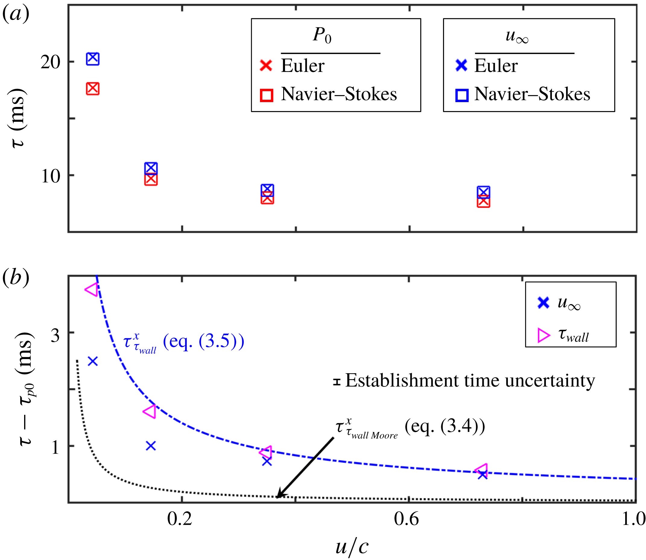
Effect of free stream velocity at constant
 $Re$
: (a)
 $\unicode[STIX]{x1D70F}_{P_{0}}$
and
 $\unicode[STIX]{x1D70F}_{u_{\infty }}$
viscous versus inviscid; (b)
 $\unicode[STIX]{x1D70F}_{u_{\infty }}^{\ast }$
and
 $\unicode[STIX]{x1D70F}_{\unicode[STIX]{x1D70F}_{wall}}^{\ast }$
versus Moore’s model, (3.4).

Figure 9(a) represents the establishment of the total pressure and the free stream velocity as a function of the free stream velocity non-dimensionalized by the speed of sound. Again Euler and URANS show the same establishment time for the mean flow boundary conditions. The faster the flow, the smaller the establishment time becomes; which is a consequence of the faster propagation of the pressure waves, which travel at
 $c+u$
, where
 $c$
is the speed of sound and
 $u$
the velocity of the medium in which they propagate.
Figure 9(b) represents the referenced establishment time of the free stream velocity and the wall shear stress. These results were compared with the trends predicted by the model of Moore (Reference Moore1951) for laminar flows, i.e. (3.4), including the laminar boundary layer thickness equation. In addition we propose a prediction model considering the results of the current research (3.5) which is achieved through a power law least squares fitting of the current results.
 $$\begin{eqnarray}\displaystyle & \displaystyle \unicode[STIX]{x1D70F}_{\unicode[STIX]{x1D70F}_{wall},Moore}=\frac{\unicode[STIX]{x1D6FF}_{laminar}^{2}}{\unicode[STIX]{x1D708}}=\frac{\left(5\sqrt{\frac{\unicode[STIX]{x1D708}x}{u_{\infty }}}\right)^{2}}{\unicode[STIX]{x1D708}}=\frac{25x}{u_{\infty }} & \displaystyle\end{eqnarray}$$
 $$\begin{eqnarray}\displaystyle & \displaystyle \unicode[STIX]{x1D70F}_{\unicode[STIX]{x1D70F}_{wall}}^{\ast }\propto \frac{1}{{u_{\infty }}^{3/4}}. & \displaystyle\end{eqnarray}$$
The final mean flow velocity is set after the passage of the last expansion wave. Then from the leading edge of the plate the boundary layer growth is convected downstream. Consequently, the faster the flow, the smaller the establishment time. Since the Reynolds number was kept constant during this analysis, all the cases had the same final boundary layer thickness. The Moore model considers that the whole plate accelerates and then all the information only travels from the leading edge to the trailing edge. Whereas in a subsonic blowdown process the free stream conditions are first set at the plate trailing edge, hence the boundary layer is already submitted to the final free stream conditions. Which implies that the only information that needs to be convected through the plate is the shape of the boundary layer, prescribed by the leading edge location.
3.4 Effect of domain length
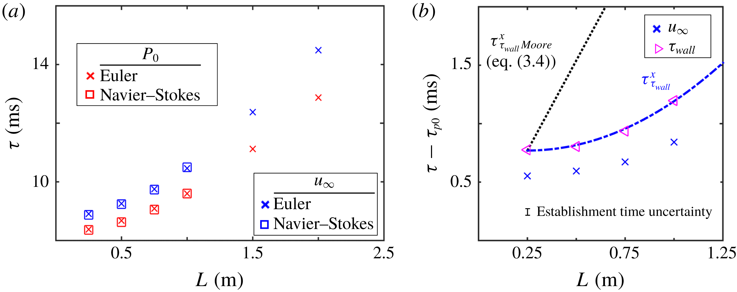
Figure 10(a) depicts the effect of the flat plate length on the establishment time of the mean flow conditions, the total pressure and free stream velocity. URANS and Euler simulations show that both methods reach the same results. Note that in the present study, the plate length is also the distance between inlet and outlet boundary condition. Thus any increase in length implies a further separation between boundaries. Larger lengths imply an increase in the distance travelled by the pressure waves.
Figure 10(b) depicts the effect of length on the referenced establishment process. The numerical establishment time data are compared against predictions obtained using the model of Moore (Moore Reference Moore1951) where the establishment time of the shear stress is directly proportionally to the plate length (
 $\unicode[STIX]{x1D70F}_{\unicode[STIX]{x1D70F}_{wall}}^{\ast }\propto x$
). In addition, we include a prediction based on a parabolic least squares fitting which reflects that the momentum boundary layer establishment should vary with the square of the plate length
 $\unicode[STIX]{x1D70F}_{\unicode[STIX]{x1D70F}_{wall}}^{\ast }\propto x^{2}$
. There are two main factors driving the increase in wall shear stress reference establishment time. First, there is a pure convective delay related with the longer distance between the leading edge and the trailing edge, increasing the boundary layer shape propagation along the plate. Additionally, the longer the plate, the thicker the boundary layer will be at the trailing edge. Hence, the diffusive propagation time across the boundary layer increases. The model of Moore describes the establishment process after the sudden start up of the plate. In this approach, the first process is the convective propagation of the information along the upstream section of the plate, followed then by the growth of the boundary to its established thickness, driven by the Reynolds number. Finally, the established main stream flow conditions diffuse across the plate. However, in the case of a sudden flow discharge over a flat plate, the boundary layer has already grown following the passage of the initial compression waves, and the adjustment of the boundary layer height required to meet the final flow velocity is significantly smaller. For this reason, the model of Moore overestimates the effect of the domain length on the referenced establishment time by a factor of 2 for a domain length of 500 mm.
Length effect: (a)
 $\unicode[STIX]{x1D70F}_{P_{0}}$
and
 $\unicode[STIX]{x1D70F}_{u_{\infty }}$
viscous versus inviscid; (b)
 $\unicode[STIX]{x1D70F}_{u_{\infty }}^{\ast }$
and
 $\unicode[STIX]{x1D70F}_{\unicode[STIX]{x1D70F}_{wall}}^{\ast }$
versus Moore.

3.5 Effect of Reynolds number and free stream temperature
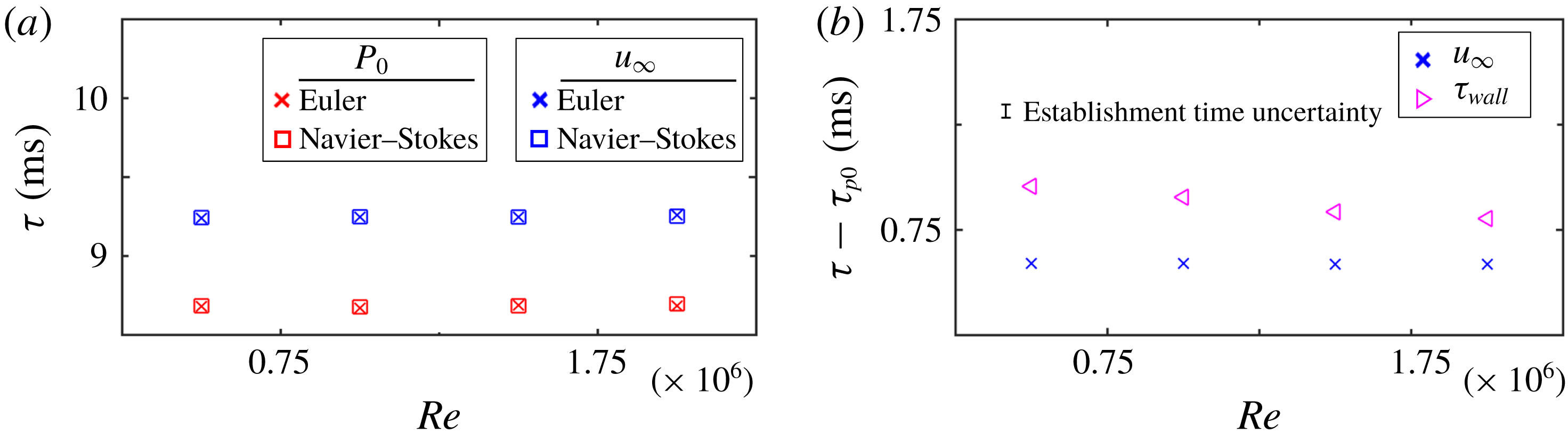
The change on the Reynolds number is achieved by modifying the static pressure level keeping constant the free stream velocity, hence isolating the effect of the free stream velocity from that of the Reynolds number. Figure 11(a) shows that there is no effect of the Reynolds number on the establishment of the mean flow conditions, pressure and free stream velocity, since it is a pure inviscid phenomenon.
Reynolds number effect: (a)
 $\unicode[STIX]{x1D70F}_{P_{0}}$
and
 $\unicode[STIX]{x1D70F}_{u_{\infty }}$
viscous versus inviscid; (b) free stream velocity referenced establishment
 $\unicode[STIX]{x1D70F}_{u_{\infty }}^{\ast }$
and wall shear stress referenced establishment
 $\unicode[STIX]{x1D70F}_{\unicode[STIX]{x1D70F}_{wall}}^{\ast }$
.

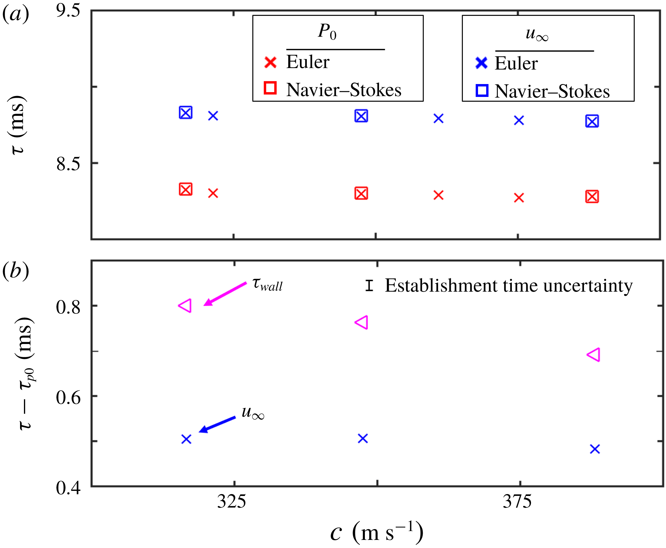
Regarding the viscous establishment, as the Reynolds number increases the boundary layer gets thinner and consequently the referenced establishment time is reduced. Figure 12(a) compares the free stream total pressure and velocity establishment based on the viscous and inviscid solver for different speeds of sound, which are achieved through free stream temperature variations. The higher the temperature the higher the speed of sound and hence the shorter the wave propagation time will be, which can be approached as
 $t_{wave\;propagation}=L/c$
.
Free stream temperature effect: (a)
 $\unicode[STIX]{x1D70F}_{P_{0}}$
and
 $\unicode[STIX]{x1D70F}_{u_{\infty }}$
viscous versus inviscid; (b)
 $\unicode[STIX]{x1D70F}_{u_{\infty }}^{\ast }$
and
 $\unicode[STIX]{x1D70F}_{\unicode[STIX]{x1D70F}_{wall}}^{\ast }$
.

Figure 12(b) represents the referenced establishment time for the wall shear stress and free stream velocity at several free stream flow temperatures. The establishment of the boundary layer is affected due to the variation of the molecular viscosity. The higher the temperature, the higher the molecular viscosity (Sutherland’s law equation (2.10)). Consequently, the diffusive process is enhanced, reducing the establishment time.
4 Thermal boundary layer establishment
The design of high speed aerospace components, including turbomachinery, nozzles, intakes, etc., requires a precise estimation of the heat flux and convective heat transfer coefficient along the surface. Short-duration facilities are cost-effective solutions to test such components at engine representative conditions. However, recent work of Johnson, Clark & Flanagan (Reference Johnson, Clark and Flanagan2007) questions the validity of such data, and in particular whether the testing is long enough to ensure the establishment of the thermal boundary layer.
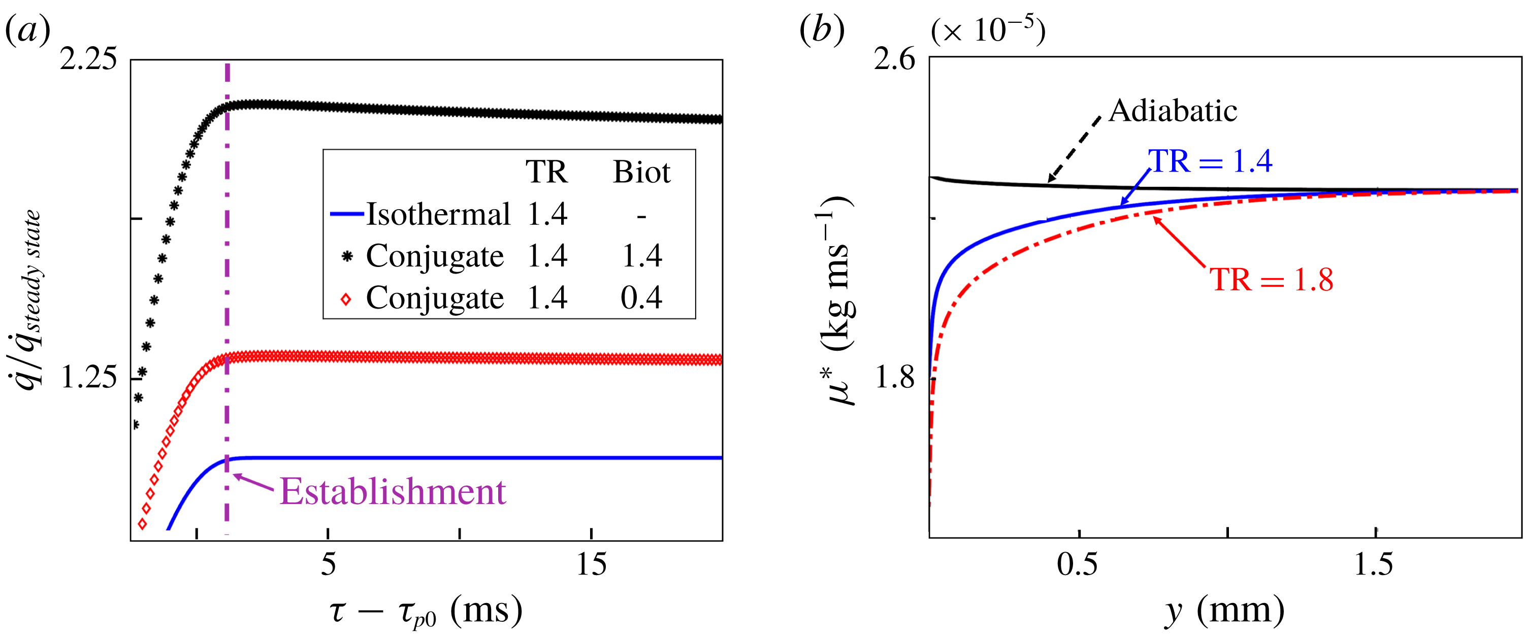
Figure 13(a) represents the evolution of the heat transfer during the blowdown predicted by a conjugate simulation. The calculations were run for two different Biot numbers and compared against a simulation run with an isothermal wall boundary condition. The Biot number expresses the ratio between the conductive heat transfer through the solid and the heat convection at its surface, equation (4.1). Hence, the Biot number describes the temperature gradient developed within the solid while being submitted to a thermal gradient at the surface exposed to contact with the gas.
 $$\begin{eqnarray}Biot=\frac{Lh}{\unicode[STIX]{x1D705}}.\end{eqnarray}$$
The heat transfer establishment takes place once the temperature distribution inside the solid reaches its steady status. This phenomena is determined by the thermal properties of the material, its conductivity, heat capacity and density effects, which could be gathered in the Fourier number.
 $$\begin{eqnarray}Fo=\frac{\unicode[STIX]{x1D6FC}t}{L^{2}}.\end{eqnarray}$$
The solid conduction is a rather slow process which delays the global establishment of the heat flux. As an example, for an aluminium slab 80 cm thick (
 $\unicode[STIX]{x1D6FC}=7.24\times 10^{-5}~\text{m}^{2}~\text{s}^{-1}$
) the mono-dimensional thermal penetration time is approximately 6.3 s. Figure 13(a) shows that, even if the internal temperature profile is far away from its steady state, the instant where they reach their maximum value coincides with the establishment time for the isothermal approach. This means that the heat transfer coefficient is established at the local wall temperature of the solid, at the same instant as if the process was isothermal. Then, the heat flux magnitude decays, in agreement with the warming up of the material. The variation of the heat flux because of a wall temperature increase takes place instantaneously due to the continuity in the surface temperature and heat flux across both domains. It can be concluded that the wall heat flux and heat transfer coefficient in a conjugate problem reaches the local steady-state condition at the same rate as was found for the isothermal approach. This is a consequence of the weak dependence of the heat transfer coefficient on the wall temperature being mainly driven by the near wall aerodynamics.
(a) Heat transfer evolution, conjugate approach; (b) molecular viscosity distribution in the boundary layer.

The effect of the temperature ratio
 $T_{0,\infty }/T_{wall}$
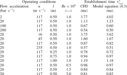
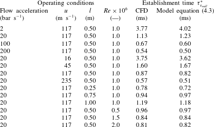
on the wall shear stress and heat flux establishment is derived from its effect on the temperature distribution, which affects the waves propagation and the molecular viscosity profile across the boundary layer. Figure 13(b) represents the molecular viscosity across the boundary layer for an adiabatic case and for two different temperature ratios, with a constant free stream temperature. It was observed that for a 40 % variation of molecular viscosity the establishment time varies by only 2 %. Considering the independent analysis performed in the previous sections and described in the figures 7(b), 9(b), 10(b), 11(b) and 12(b), and using a least square fit, we could derive an expression to estimate the momentum boundary layer reference establishment time.
 $$\begin{eqnarray}\unicode[STIX]{x1D70F}_{\unicode[STIX]{x1D70F}_{wall}}^{\ast }=\sqrt{\unicode[STIX]{x1D707}}\frac{4.2}{Re^{1/8}TR}\frac{1}{(u_{\infty }/c)^{3/4}}\frac{1}{\sqrt{\unicode[STIX]{x0394}P_{0}/\unicode[STIX]{x1D6E5}_{start\text{-}up}}}\left(1+0.15\left(\frac{L^{2}}{L_{ref}^{2}}\right)\right),\end{eqnarray}$$
where the reference length (
 $L_{ref}$
) is 0.5 m. The accuracy of the given expression is tested against the establishment times found in current research. The range of conditions are:
 $$\begin{eqnarray}\displaystyle & 5\times 10^{5}<Re<2\times 10^{6}; & \displaystyle\end{eqnarray}$$
 $$\begin{eqnarray}\displaystyle & 0.7<TR<1.4; & \displaystyle\end{eqnarray}$$
 $$\begin{eqnarray}\displaystyle & 2<\unicode[STIX]{x0394}P_{0}/\unicode[STIX]{x1D6E5}_{start\text{-}up}<200; & \displaystyle\end{eqnarray}$$
 $$\begin{eqnarray}\displaystyle & 0.01<M<0.75. & \displaystyle\end{eqnarray}$$
The maximum deviation of the referenced establishment predictions based on (4.3) from the numerical blowdown results are below 10 % and the confidence level is 92 %. Table 4 summarizes all of the investigated test cases, the flow operating conditions as well as a comparison of the CFD with the predicted establishment using (4.3).
Comparison of thermal and momentum boundary layer establishment times.

Establishment time for all investigated cases predicted by CFD and by the proposed model, equation (4.3).
Regarding the thermal boundary layer, the ratio between the thermal and momentum boundary layer height is related to the Prandtl number, for air
 $Pr\approx 0.72$
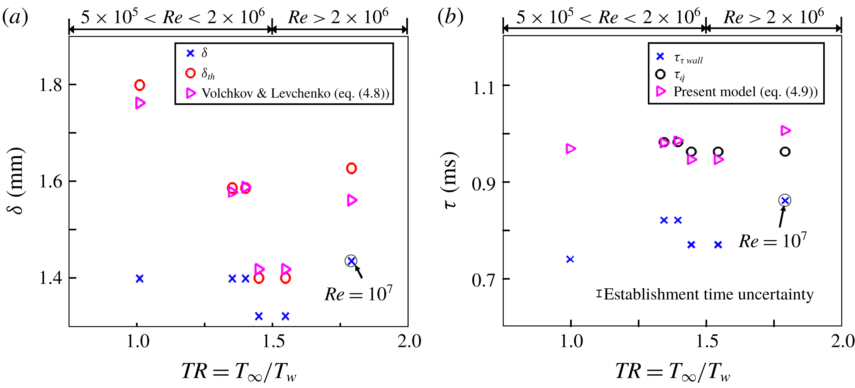
the thermal boundary layer is thicker than the momentum one. Figure 14(a) represents the CFD momentum and thermal boundary layer thickness for a variety of wall-to-fluid temperature ratios and Reynolds numbers. The URANS results are compared with the correlation proposed by Volchkov & Levchenko (Reference Volchkov and Levchenko1965) (4.8).
 $$\begin{eqnarray}\unicode[STIX]{x1D6FF}_{th}=\frac{\unicode[STIX]{x1D6FF}}{\left({\displaystyle \frac{Re^{0.25}Pr^{0.75}}{0.1115}}St\right)^{7}}.\end{eqnarray}$$
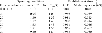
Figure 14(b) reports the establishment times of the wall shear stress and of the heat flux as a function of the temperature ratio between the free stream and the wall. This figure shows that the establishment time of the thermal boundary layer is approximately one millisecond slower than the establishment of the momentum boundary layer, over a wide range of Reynolds number and temperature ratios. Inspired by the model of Volchkov and Levchenko (4.8), we have determined a new expression to predict the thermal boundary layer establishment using a power law least-square fitting of the current blowdown CFD-based data. The prediction of the thermal boundary layer establishment time is based on four principal parameters:
(i) the establishment of the momentum,
$\unicode[STIX]{x1D70F}_{\unicode[STIX]{x1D70F}_{wall}}^{\ast }$
;(ii) the Reynolds number (
$Re$
, based on the axial position and the free stream velocity);(iii) Prandtl number, (
$Pr$
);(iv) local Nusselt number, (
$Nu$
, based on the local heat transfer coefficient and fluid properties near the wall).


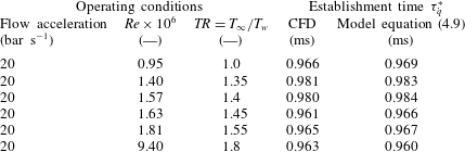
Table 5 summarizes the different temperature ratios analysed with their flow operating conditions and it presents a comparison of the CFD establishment times with the prediction equation (4.9). The working fluid in all the cases was dry air and the free stream temperature ranged from 250 K up to 380 K. Consequently, the range of Prandtl number considered in this study remains between 0.69 and 0.72. In terms of Nusselt numbers, we explored cases from a few hundred up to 5000.
 $$\begin{eqnarray}\unicode[STIX]{x1D70F}_{\dot{q}}^{\ast }=\frac{\unicode[STIX]{x1D70F}_{\unicode[STIX]{x1D70F}_{wall}}^{\ast }}{\left({\displaystyle \frac{Nu}{0.1115Re^{0.78}Pr^{0.25}}}\right)^{7}}.\end{eqnarray}$$
Thermal establishment time for several cases predicted by CFD and by the proposed model, equation (4.9).
5 Conclusions
The inception of the thermal boundary layer and its dynamic response edicts the performance of heat exchangers and constrains the operational envelope of fluid machinery. Aiming the characterization of the near wall flow region under sudden flow start ups this paper presents a study of the establishment times of the turbulent momentum and thermal boundary layer under adiabatic, isothermal and full conjugate conditions. The establishment of the turbulent boundary layer during a subsonic blowdown process was analysed by performing parametric studies of the main factors describing the flow conditions and the transient evolution. Over 80 different blowdown processes were run using unsteady Reynolds averaged Navier–Stokes simulations, which required more than 20 months of CPU time.
The establishment sequence is described and compared to previously proposed analytical approaches valid for laminar flows. The different factors comprised: total pressure slope of the transient evolution, Reynolds number, free stream velocity, free stream temperature and wall-to-fluid temperature ratio. Each one of these parameters has multiple implications for the establishment. Through their isolated analysis we could determine a general equation to predict the overall establishment time after a sudden start up of the flow. The establishment of the momentum boundary layer could range from 5 ms down to fractions of a millisecond after the settlement of the mean flow for different start-up cases. A procedure to study the establishment of both thermal and momentum boundary layers in a subsonic blowdown process is described. In addition to the general referenced establishment approximation, we propose a new way to assess the turbulent boundary layer establishment which improves the current tools available in the literature for subsonic operation.
The establishment times of the mean flow boundary conditions, total pressure and core flow velocity were analysed using URANS and Euler simulations. The agreement between the URANS and Euler simulations indicates that the mean flow establishment is a purely inviscid phenomenon; so viscous effects can be neglected when analysing the mean flow establishment. After the establishment of the mean flow, the new free stream conditions are diffused across the boundary layer height. This paper provides a correlation that predicts the establishment time of the thermal boundary layer over a wide range of flow conditions. This establishment time is required to select the adequate time window for deriving the heat flux from experimental data obtained in short-duration facilities. Heat flux data obtained from time windows prior to the full establishment of the thermal boundary layer, will result in an overestimation of the heat flux compared to the steady CFD evaluation, which was previously observed by Johnson et al. (Reference Johnson, Clark and Flanagan2007). Unfortunately this may be the case in numerous short duration facilities, where the test duration may be too brief to ensure the establishment of the thermal boundary layer. Therefore, the data presented in this paper can be used to design heat transfer facilities, as well as to select the correct time window for post-processing of the heat flux data. Furthermore, in turbomachinery flows the boundary layer is periodically disrupted by relatively high frequency events, with typical blade passing frequencies of the order of kHz. In turbine flows, the wall shear stress and heat flux can deviate considerably from steady mean flow predictions
For the range of Reynolds numbers explored in this research the thermal boundary layer will require around
 $300~\unicode[STIX]{x03BC}\text{s}$
more than the momentum boundary layer establishment to reach its final status for air Prandtl numbers around 0.72. Accounting for the thermal establishment delay, we propose an equation to predict the thermal boundary layer establishment time based on the momentum boundary layer establishment and various mean flow properties. Finally, making use of conjugate simulations, it is confirmed that, independently of the final mono-dimensional temperature profile inside of the solid, the heat transfer coefficient will be established at the same rate as for an isothermal condition. This is significant because it reveals the capability of measuring accurate heat transfer properties without requiring full thermal equilibrium. This manuscript is of relevance to aero-thermal designers concerned with convective heat fluxes. The strategy and results presented here can be used to develop effective control of the time-dependent dynamics of attached boundary layers and allow heat transfer enhancement or abatement.
Acknowledgements
This material is based upon work supported by the Air Force Office of Scientific Research, Air Force Material Command, USAF under Award no. FA9550-16-1-0120.
Symbol
-
$A\,=$
Cst. heat transfer equation Volchkov
-
$avg\,=$
Averaged
-
$b\,=$
Plate thickness
-
$Bi\,=$
Euler number
$={\displaystyle \frac{h}{l\unicode[STIX]{x1D705}}}$
-
$c\,=$
Speed of sound
$(\text{m}~\text{s}^{-1})$
-
$c_{p}\,=$
Heat capacity
$(\text{J}~\text{kg}^{-1}~\text{K}^{-1})$
-
$e\,=$
Total Energy
$(\text{m}^{2}~\text{s}^{-2})$
-
$Eu\,=$
Euler number
$={\displaystyle \frac{\unicode[STIX]{x0394}P}{\unicode[STIX]{x1D70C}u_{\infty }^{2}}}$
-
$Fo\,=$
Fourier number
$={\displaystyle \frac{\unicode[STIX]{x1D6FC}}{b^{2}}}$
-
$F\,=$
Navier–Stokes equations inviscid flux vectors
-
$G\,=$
Navier–Stokes equations viscous flux vectors
-
$h\,=$
Heat transfer coefficient
$(\text{W}~\text{m}^{-2}~\text{K}^{-1})$
-
$L\,=$
Length (m)
-
$l_{t}\,=$
Turbulent length scale (m)
-
$M\,=$
Mach number
-
$P\,=$
Pressure (Pa)
-
$Pr\,=$
Prandtl number,
$Pr={\displaystyle \frac{\unicode[STIX]{x1D707}c_{p}}{\unicode[STIX]{x1D705}}}$
-
$\dot{q}\,=$
Heat transfer
$(\text{W}~\text{m}^{-2})$
-
$Re\,=$
Reynolds number
$Re={\displaystyle \frac{ux}{\unicode[STIX]{x1D708}}}$
-
$St\,=$
Stanton
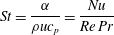
$St={\displaystyle \frac{\unicode[STIX]{x1D6FC}}{\unicode[STIX]{x1D70C}uc_{p}}}={\displaystyle \frac{Nu}{Re\,Pr}}$
-
$T\,=$
Temperature (K)
-
$Tu\%\,=$
Turbulence intensity (—)
-
$TR\,=$
Temperature ratio
${\displaystyle \frac{T_{\infty }}{T_{w}}}$
-
$u\,=$
Velocity (
$\text{m}~\text{s}^{-1}$
)-
$V_{1}\,=$
Euler equations inviscid flux vector
-
$x\,=$
Axial position (m)
-
$y\,=$
Normal position (m)
-
$W\,=$
Euler equation dependent variable vector




Greek symbols
-
$\unicode[STIX]{x1D6FC}\,=$
Thermal diffusivity
$(\text{m}^{2}~\text{s}^{-1})$
-
$\unicode[STIX]{x1D6FF}\,=$
Boundary layer thickness (m)
-
$\unicode[STIX]{x1D6FF}^{\ast }\,=$
Boundary layer displacement thickness (m)
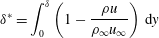
$\unicode[STIX]{x1D6FF}^{\ast }=\displaystyle \int _{0}^{\unicode[STIX]{x1D6FF}}\left(1-{\displaystyle \frac{\unicode[STIX]{x1D70C}u}{\unicode[STIX]{x1D70C}_{\infty }u_{\infty }}}\right)\,\text{d}y$
-
$\unicode[STIX]{x1D6FF}_{th}\,=$
Thermal boundary layer thickness (m)
-
$\unicode[STIX]{x1D702}\,=$
Boundary layer similarity variable
$\unicode[STIX]{x1D702}=y\sqrt{u_{\infty }/(\unicode[STIX]{x1D708}x)}$
-
$\unicode[STIX]{x1D703}\,=$
Boundary layer momentum thickness (m)
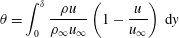
$\unicode[STIX]{x1D703}=\displaystyle \int _{0}^{\unicode[STIX]{x1D6FF}}{\displaystyle \frac{\unicode[STIX]{x1D70C}u}{\unicode[STIX]{x1D70C}_{\infty }u_{\infty }}}\left(1-{\displaystyle \frac{u}{u_{\infty }}}\right)\,\text{d}y$
-
$\unicode[STIX]{x1D6FE}\,=$
Heat capacity ratio
-
$\unicode[STIX]{x1D705}\,=$
Thermal conductivity
$(\text{W}~\text{m}^{-1}~\text{K}^{-1})$
-
$\unicode[STIX]{x1D6F7}\,=$
dilatation
$(\text{s}^{-1})$
-
$\unicode[STIX]{x1D707}\,=$
Kinematic viscosity
$(\text{kg}~\text{m}^{-1}~\text{s}^{-1})$
-
$\unicode[STIX]{x1D708}\,=$
Dynamic viscosity
$(\text{m}^{2}~\text{s}^{-1})$
-
$\unicode[STIX]{x1D70C}\,=$
Density
$(\text{kg}~\text{m}^{-3})$
-
$\unicode[STIX]{x1D70F}\,=$
Establishment time (s)
-
$\unicode[STIX]{x1D70F}_{wall}\,=$
Wall shear stress (Pa)






Subscripts and superscripts
-
$0\,=$
Total or stagnant quantity
-
$b\,=$
Solid bottom wall
-
$c\,=$
Characteristic time
-
$\infty \,=$
Free stream conditions
-
$w\,=$
Wall conditions
-
$s\,=$
Solid
-
$LE\,=$
Leading edge
-
$TE\,=$
Trailing edge