1 Introduction
The mixing of convected contaminants is an essential characteristic of a turbulent flow, in which the large-scale structures play an important role in transporting the passive scalar, while small scales act to mix the scalar with the ambient fluid (Tennekes & Lumley Reference Tennekes and Lumley1972). Small-scale mixing is an important process in several applications, including turbulent combustion, air pollution dissipation, water processing, etc. (e.g. Shraiman & Siggia Reference Shraiman and Siggia2000; Warhaft Reference Warhaft2000). An improved knowledge of the mean scalar dissipation rate is essential for the comprehension of passive scalar mixing. The mean dissipation rate of a passive scalar (or temperature in the present study) is defined as
 $\overline{\unicode[STIX]{x1D712}}\equiv \unicode[STIX]{x1D705}\overline{\unicode[STIX]{x1D703}_{,i}\,\unicode[STIX]{x1D703}_{,i}}~(=\unicode[STIX]{x1D705}(\overline{\unicode[STIX]{x1D703}_{,1}\unicode[STIX]{x1D703}_{,1}}+\overline{\unicode[STIX]{x1D703}_{,2}\unicode[STIX]{x1D703}_{,2}}+\overline{\unicode[STIX]{x1D703}_{,3}\unicode[STIX]{x1D703}_{,3}}))$
, where an overbar indicates a time-averaged quantity. Here,
 $\unicode[STIX]{x1D705}$
is the thermal diffusivity;
 $\unicode[STIX]{x1D703}$
denotes the temperature fluctuation, and
 $\unicode[STIX]{x1D703}_{,i}\equiv \unicode[STIX]{x2202}\unicode[STIX]{x1D703}/\unicode[STIX]{x2202}x_{i}$
,
 $i=1,2$
and 3 representing the streamwise, lateral and spanwise directions respectively, which are used interchangeably with
 $x$
,
 $y$
and
 $z$
.
The dissipation process of the scalar variance is closely related to that of the turbulent kinetic energy of the transporting velocity field. Antonia et al. (Reference Antonia, Ould-Rouis, Anselmet and Zhu1997) generalized Kolmogorov’s ‘
 $4/5$
law’ and showed that the third-order moments
 $\overline{\unicode[STIX]{x1D6FF}u(\unicode[STIX]{x1D6FF}q)^{2}}$
and
 $\overline{\unicode[STIX]{x1D6FF}u(\unicode[STIX]{x1D6FF}\unicode[STIX]{x1D703})^{2}}$
, where
 $(\unicode[STIX]{x1D6FF}q)^{2}=(\unicode[STIX]{x1D6FF}u)^{2}+(\unicode[STIX]{x1D6FF}v)^{2}+(\unicode[STIX]{x1D6FF}w)^{2}$
and
 $\unicode[STIX]{x1D6FF}\unicode[STIX]{x1D6FC}=\unicode[STIX]{x1D6FC}(x_{1}+r_{1})-\unicode[STIX]{x1D6FC}(x_{1})$
(
 $\unicode[STIX]{x1D6FC}$
stands for either velocity fluctuations
 $u$
,
 $v$
,
 $w$
or
 $\unicode[STIX]{x1D703}$
, and
 $r_{1}$
is the separation distance in the streamwise direction), have similar forms in the inertial range, i.e. the length scale range of turbulent motions which resides between the energy containing range and the dissipation range (Pope Reference Pope2001), namely
 $$\begin{eqnarray}\displaystyle & \displaystyle \overline{\unicode[STIX]{x1D6FF}u(\unicode[STIX]{x1D6FF}q)^{2}}=-{\textstyle \frac{4}{3}}\overline{\unicode[STIX]{x1D716}}r_{1}, & \displaystyle\end{eqnarray}$$
 $$\begin{eqnarray}\displaystyle & \displaystyle \overline{\unicode[STIX]{x1D6FF}u(\unicode[STIX]{x1D6FF}\unicode[STIX]{x1D703})^{2}}=-{\textstyle \frac{4}{3}}\overline{\unicode[STIX]{x1D712}}r_{1}. & \displaystyle\end{eqnarray}$$
Here,
 $\overline{\unicode[STIX]{x1D716}}$
is the mean turbulent kinetic energy dissipation rate. In the dissipation range, the transport equations for
 $\overline{(\unicode[STIX]{x1D6FF}q)^{2}}$
and
 $\overline{(\unicode[STIX]{x1D6FF}\unicode[STIX]{x1D703}^{2})}$
reduce, in the limit of
 $r_{1}\rightarrow 0$
, to
 $$\begin{eqnarray}\displaystyle & \displaystyle \overline{\frac{\unicode[STIX]{x2202}u}{\unicode[STIX]{x2202}x_{1}}\left(\frac{\unicode[STIX]{x2202}q}{\unicode[STIX]{x2202}x_{1}}\right)^{\!2}}=-\frac{2}{3}\unicode[STIX]{x1D708}\overline{\left(\frac{\unicode[STIX]{x2202}^{2}q}{\unicode[STIX]{x2202}x_{1}^{2}}\right)^{\!2}}, & \displaystyle\end{eqnarray}$$
 $$\begin{eqnarray}\displaystyle & \displaystyle \overline{\frac{\unicode[STIX]{x2202}u}{\unicode[STIX]{x2202}x_{1}}\left(\frac{\unicode[STIX]{x2202}\unicode[STIX]{x1D703}}{\unicode[STIX]{x2202}x_{1}}\right)^{\!2}}=-\frac{2}{3}\unicode[STIX]{x1D705}\overline{\left(\frac{\unicode[STIX]{x2202}^{2}\unicode[STIX]{x1D703}}{\unicode[STIX]{x2202}x_{1}^{2}}\right)^{\!2}}, & \displaystyle\end{eqnarray}$$
where
 $\unicode[STIX]{x1D708}$
is the kinematic viscosity. The similarity between (1.3) and (1.4) (and also (1.1) and (1.2)), which is underpinned by the Navier–Stokes and heat transport equations as well as experimental results in a plane wake (Antonia et al.
Reference Antonia, Ould-Rouis, Anselmet and Zhu1997), implies a possible similarity between the two dissipative processes. Antonia, Djenidi & Danaila (Reference Antonia, Djenidi and Danaila2014) showed that the collapse of the dissipative range on Kolmogorov scales does not require either of the two major assumptions (the Reynolds number is very large and local isotropy is satisfied) in Kolmogorov’s first similarity hypothesis. Further, the transport equations of the scalar gradient variance
 $\overline{\unicode[STIX]{x1D703}_{,i}\,\unicode[STIX]{x1D703}_{,i}}$
and enstrophy
 $\overline{\unicode[STIX]{x1D714}_{i}\unicode[STIX]{x1D714}_{i}}$
(
 $\equiv \overline{\unicode[STIX]{x1D714}_{1}\unicode[STIX]{x1D714}_{1}}+\overline{\unicode[STIX]{x1D714}_{2}\unicode[STIX]{x1D714}_{2}}+\overline{\unicode[STIX]{x1D714}_{3}\unicode[STIX]{x1D714}_{3}}$
, where
 $\unicode[STIX]{x1D714}_{i}$
is the vorticity fluctuation in the
 $i$
direction) are similar in form (Corrsin Reference Corrsin1953; Abe, Antonia & Kawamura Reference Abe, Antonia and Kawamura2009), where
 $\overline{\unicode[STIX]{x1D703}_{,i}\,\unicode[STIX]{x1D703}_{,i}}$
is hereafter referred to as the mean scalar dissipation rate since
 $\unicode[STIX]{x1D705}$
, like
 $\unicode[STIX]{x1D708}$
, is constant and
 $\overline{\unicode[STIX]{x1D714}_{i}\unicode[STIX]{x1D714}_{i}}$
is a good surrogate for the turbulent energy dissipation rate since
 $\unicode[STIX]{x1D708}\overline{\unicode[STIX]{x1D714}_{i}\unicode[STIX]{x1D714}_{i}}$
is a good approximation to the dissipation rate of the turbulent kinetic energy in a plane wake, at least for
 $x/d\geqslant 20$
(Lefeuvre et al.
Reference Lefeuvre, Thiesset, Djenidi and Antonia2014). This surrogacy is exact for homogeneous turbulence (e.g. Antonia, Kim & Browne Reference Antonia, Kim and Browne1991). Unfortunately, it is a challenge to measure simultaneously the three components of the vorticity vector (Antonia & Rajagopalan Reference Antonia and Rajagopalan1990; Marasli, Nguyen & Wallace Reference Marasli, Nguyen and Wallace1993; Wallace & Foss Reference Wallace and Foss1995) and especially to capture experimentally this vector simultaneously with the temperature gradient vector. As a result, previous data on the correlation between the enstrophy and the scalar dissipation rate have been obtained mainly numerically. Using direct numerical simulation data, Abe et al. (Reference Abe, Antonia and Kawamura2009) studied the correlation between the scalar dissipation field and the vorticity field of a fully developed turbulent channel flow and uncovered a close similarity between different components of
 $\unicode[STIX]{x1D703}_{,i}$
and
 $\unicode[STIX]{x1D714}_{i}$
in the inner region of the flow, which results from the almost perfect correspondence between momentum and thermal streaks near the wall. Using the same database, Antonia, Abe & Kawamura (Reference Antonia, Abe and Kawamura2009) noticed a reasonable similarity between spectra corresponding to the enstrophy and scalar dissipation rate as well as between velocity and temperature spectra; the latter similarity was not unexpected given the importance of the mean velocity and temperature gradients, as in the boundary layer flow first considered by Fulachier & Dumas (Reference Fulachier and Dumas1971, Reference Fulachier and Dumas1976).
With the exception of Antonia et al. (Reference Antonia, Abe and Kawamura2009), very little has been reported in the literature on the relationship between the scalar dissipation rate and the enstrophy. This is in contrast to the similarity between the scalar variance and the turbulent kinetic energy, which has drawn considerable attention from researchers. The temperature fluctuation
 $\unicode[STIX]{x1D703}$
is lamellar in nature, while the velocity fluctuation vector
 $\boldsymbol{q}$
is solenoidal. Therefore, a direct similarity between
 $\unicode[STIX]{x1D703}$
and
 $\boldsymbol{q}$
may not exist. Nevertheless, it is reasonable to explore the similarity between the scalar variance
 $\overline{\unicode[STIX]{x1D703}^{2}}$
and the mean turbulent kinetic energy
 $\overline{q^{2}}$
, which are both scalar quantities. This similarity should be as plausible as the Reynolds analogy from a physical point of view. Fulachier & Dumas (Reference Fulachier and Dumas1971, Reference Fulachier and Dumas1976) first observed the similarity between the
 $\unicode[STIX]{x1D703}$
and
 $\boldsymbol{q}$
spectra across most of the turbulent flat-plate boundary layer. Fulachier & Antonia (Reference Fulachier and Antonia1984) further established that the transport equations for
 $\overline{\unicode[STIX]{x1D703}^{2}}$
and
 $\overline{q^{2}}$
are formally analogous when the Prandtl number
 $Pr=1$
, except for the pressure term in the equation for
 $\overline{q^{2}}$
, and verified this similarity in other turbulent shear flows, including the plane far wake of a cylinder, and nearly homogeneous turbulence with uniform mean velocity and mean temperature gradients. It should be noted that the spectral similarity can provide useful insight into the flow physics. For example, Antonia et al. (Reference Antonia, Abe and Kawamura2009) observed near the wall of a turbulent channel flow that the spanwise wavenumber
 $(k_{z})$
or wavenumber of the peak in both of the spectra
 $k_{z}F_{q}(k_{z})$
and
 $k_{z}F_{\unicode[STIX]{x1D703}}(k_{z})$
, which make the major contributions to
 $\overline{q^{2}}$
and
 $\overline{\unicode[STIX]{x1D703}^{2}}$
, corresponds to a spanwise wavelength of
 $l_{z}^{\dagger }=104.7$
, where
 $\dagger$
denotes normalization with wall units. This wavelength coincides closely with the averaged spanwise separation, i.e.
 $\unicode[STIX]{x1D706}_{z}^{\dagger }\approx 100$
, between the low-speed streaks (e.g. Tomkins & Adrian Reference Tomkins and Adrian2003). It is worth pointing out that the production of
 $\overline{\unicode[STIX]{x1D703}^{2}}$
and
 $\overline{q^{2}}$
, for example via the interaction between
 $\overline{uv}$
and
 $\unicode[STIX]{x2202}\overline{U}/\unicode[STIX]{x2202}y$
or between
 $\overline{v\unicode[STIX]{x1D703}}$
and
 $\unicode[STIX]{x2202}\overline{\unicode[STIX]{x1D6E9}}/\unicode[STIX]{x2202}y$
(Fulachier & Antonia Reference Fulachier and Antonia1984), must be maintained for this spectral similarity to be valid; otherwise, the similarity breaks down, as, for example, in grid turbulence (see chap. 7 of Chassaing et al.
Reference Chassaing, Antonia, Anselmet, Joly and Sarkar2002). In general, the production of
 $\overline{\unicode[STIX]{x1D703}^{2}}$
and
 $\overline{q^{2}}$
(or ‘forcing’) at low wavenumbers will allow (1.1) and (1.2) to be valid at lower Reynolds numbers than in the absence of ‘forcing’ (see, for example, Watanabe & Gotoh Reference Watanabe and Gotoh2004 and Antonia & Burattini Reference Antonia and Burattini2006). One expects a similar behaviour for the spectra. In a boundary layer or a channel flow, the wall, if heated, acts as a source of
 $\overline{\unicode[STIX]{x1D703}^{2}}$
and
 $\overline{q^{2}}$
, and the spectral similarity is well supported (Antonia & Kim Reference Antonia and Kim1991; Antonia et al.
Reference Antonia, Abe and Kawamura2009). In free shear flows, such as circular and plane jets and the far wake at some distance away from the centreline, the mean velocity and temperature gradients provide sufficient forcing for the similarity to work reasonably well (e.g. Fulachier & Antonia Reference Fulachier and Antonia1983; Chua & Antonia Reference Chua and Antonia1991).
In all previous studies, the similarity between either the small scales
 $\overline{\unicode[STIX]{x1D714}_{i}\unicode[STIX]{x1D714}_{i}}$
and
 $\overline{\unicode[STIX]{x1D703}_{,i}\,\unicode[STIX]{x1D703}_{,i}}$
or the energy containing scales
 $\overline{q^{2}}$
and
 $\overline{\unicode[STIX]{x1D703}^{2}}$
has been examined in approximately self-preserving or fully developed turbulent flows (e.g. Fulachier & Dumas Reference Fulachier and Dumas1976; Fulachier & Antonia Reference Fulachier and Antonia1984; Antonia et al.
Reference Antonia, Abe and Kawamura2009). There has been no attempt to date to carry out such a study in the turbulent intermediate wake (
 $10\leqslant x/d\leqslant 40$
) of a circular cylinder of diameter
 $d$
, which is developing and features the formation, decay and subsequent disappearance of the strong coherent structures (the Kármán vortex street and the streamwise ribs). Thiesset, Danaila & Antonia (Reference Thiesset, Danaila and Antonia2014) revealed that the dynamical influence of these coherent motions is perceptible even at the smallest scales whose energy is enhanced when the coherent strain is maximum. Matsumura & Antonia (Reference Matsumura and Antonia1993) showed that heat is mostly contained within the Kármán vortex in the intermediate wake (
 $x/d=10$
to 40), which is quite different from the picture of the flow near a wall, in which there is an almost perfect correspondence between velocity and thermal streaks (Abe et al.
Reference Abe, Antonia and Kawamura2009). As such, several fundamental and interesting questions emerge. Is the similarity between
 $\overline{\unicode[STIX]{x1D714}_{i}\unicode[STIX]{x1D714}_{i}}$
and
 $\overline{\unicode[STIX]{x1D703}_{,i}\unicode[STIX]{x1D703}_{,i}}$
, as well as that between
 $\overline{q^{2}}$
and
 $\overline{\unicode[STIX]{x1D703}^{2}}$
, still valid in the present flow? What is the effect of the highly coherent structures on the similarity? How does the quality of the similarity vary as the coherent structures undergo substantial changes as the distance from the cylinder increases? These questions are as yet unanswered. The present work aims at providing answers to these questions, in the context of two types of comparison between the turbulent velocity field and the passive scalar field, one between
 $\overline{\unicode[STIX]{x1D703}_{,i}\,\unicode[STIX]{x1D703}_{,i}}$
and
 $\overline{\unicode[STIX]{x1D714}_{i}\unicode[STIX]{x1D714}_{i}}$
, representing the small-scale structures, and the other between
 $\overline{\unicode[STIX]{x1D703}^{2}}$
and
 $\overline{q^{2}}$
, mainly due to the large-scale structures. Use is made of a multiple hot wire probe (Zhou, Antonia & Chua Reference Zhou, Antonia and Chua2002a
; Chen, Zhou & Zhou Reference Chen, Zhou, Zhou and Antonia2016) to measure simultaneously the three components of velocity and vorticity as well as the full temperature gradient vector at nominally the same point. This allows the scalar dissipation rate and enstrophy to be estimated without assuming isotropy.
The paper is organized as follows. Experimental details are given in § 2. Section 3 introduces the phase-averaging technique used to extract the coherent structures from the flow. The mean velocity and temperature field is shown in § 4. The similarity between the scalar dissipation rate and the enstrophy is examined in both the spectral and physical spaces in § 5, and so is that between the passive scalar variance and the turbulent kinetic energy in § 6. The latter is done by separately considering the contributions from the large-scale coherent structures and those of the remaining scales to
 $\overline{\unicode[STIX]{x1D714}_{i}\unicode[STIX]{x1D714}_{i}}$
,
 $\overline{\unicode[STIX]{x1D703}_{,i}\,\unicode[STIX]{x1D703}_{,i}}$
as well as
 $\overline{q^{2}}$
and
 $\overline{\unicode[STIX]{x1D703}^{2}}$
. The ratio of the time scales
 $\overline{\unicode[STIX]{x1D703}^{2}}/(\unicode[STIX]{x1D705}\overline{\unicode[STIX]{x1D703}_{,i}\,\unicode[STIX]{x1D703}_{,i}})$
and
 $\overline{q^{2}}/(\unicode[STIX]{x1D708}\overline{\unicode[STIX]{x1D714}_{i}\unicode[STIX]{x1D714}_{i}})$
associated with the scalar and velocity fields as well as the behaviour of the turbulent Prandtl number
 $Pr_{t}$
are examined in § 7, and the major conclusions are outlined in § 8.
2 Experimental details
Experiments were conducted in an open-loop wind tunnel with a working section of 1.2 (width)
 $\times$
0.8 m (height) and of 2.0 m length. The free-stream longitudinal turbulence intensity was smaller than 0.5 %, and the flow was uniform to within 0.2 % in the working section in the absence of the cylinder. A circular cylinder with a diameter of
 $d=12.7~\text{mm}$
was used to generate the wake. The cylinder was aligned horizontally at the centre of the test section and was supported rigidly by two aluminium sharp edged end plates. The cylinder was made of a 110 cm long smooth brass tube with an outer diameter of 12.7 mm, i.e. with an aspect ratio of approximately 87 and a blockage ratio of 1.6 %. A coiled heating wire with a diameter of approximately 0.5 mm was inserted into a ceramic tube, which was put inside the cylinder as a heating element. The free-stream velocity
 $U_{1}$
was
 $3.0~\text{m}~\text{s}^{-1}$
, corresponding to a Reynolds number
 $Re~(\equiv U_{1}d/\unicode[STIX]{x1D708})$
of
 $2.5\times 10^{3}$
. Measurements were conducted within the cylinder mid-span plane at downstream locations of
 $x/d=10,20$
and 40, where
 $x$
is the streamwise distance from the cylinder axis. The unheated cylinder wake has been shown to be statistically symmetrical about the centreline, e.g. by Zhou et al. (Reference Zhou, Razali, Zhou, Chua and Cheng2009). As a result, the present measurements were made only on one side of the centreline, i.e.
 $y/d=-0.2{-}2.8$
at
 $x/d=10$
and 20 and
 $-0.2$
–4.3 at
 $x/d=40$
, with a transverse measurement increment of approximately
 $0.2d$
for all
 $x/d$
locations, except the region near the free stream at
 $x/d=40$
where the increment was
 $0.4d$
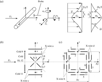
. The coordinate system and some symbols are defined in figure 1(a). The average temperature of the cylinder surface was estimated to be roughly
 $28\,^{\circ }\text{C}$
and the maximum mean temperature excess
 $\unicode[STIX]{x1D6E9}_{0}$
, relative to the ambient fluid, was approximately
 $1.6\,^{\circ }\text{C}$
,
 $1.5\,^{\circ }\text{C}$
and
 $1.3\,^{\circ }\text{C}$
on the centreline for
 $x/d=10$
, 20 and 40 respectively. This excess was small enough to avoid any buoyancy effects, and hence to allow the temperature to be treated as a passive scalar.
(a) Experimental arrangement, coordinate system and definition sketch; (b) and (c) side and front views of the vorticity probe (
 $\unicode[STIX]{x1D6FD}=50^{\circ }$
).

A probe consisting of four X-wires (figure 1
b) and four cold wires was used to measure simultaneously the velocity and temperature fluctuations. Two of the X-wires, b and d, were aligned in the
 $x{-}y$
plane and separated by
 $\unicode[STIX]{x0394}z=2.7~\text{mm}$
in the
 $z$
direction; the other two, a and c, were in the
 $x{-}z$
plane and separated by
 $\unicode[STIX]{x0394}y=2.0~\text{mm}$
in the
 $y$
direction. Four cold wires were orientated orthogonally to the plane of the cross-wire and placed approximately 1 mm upstream of the vorticity probe. The separations
 $\unicode[STIX]{x0394}y$
and
 $\unicode[STIX]{x0394}z$
between the opposite cold wires were 2.5 mm and 2.2 mm respectively. The fluctuations
 $u$
,
 $v$
,
 $w$
and
 $\unicode[STIX]{x1D703}$
captured by this probe may be considered to be obtained at nominally the same point in space.
Both hot and cold wires were etched from Wollaston (Pt–10 % Rh) wires, with active lengths of approximately
 $200d_{w}$
and
 $800d_{w}$
respectively, where
 $d_{w}$
is the diameter of the wires, namely
 $2.5~\unicode[STIX]{x03BC}\text{m}$
for the hot wires and
 $1.27~\unicode[STIX]{x03BC}\text{m}$
for the cold wires. The hot wires were operated on constant-temperature circuits, built in-house, at an overheat ratio of 1.5. The cold wires were operated with constant-current (0.1 mA) circuits. The probe was calibrated at the centreline of the tunnel using a Pitot static tube connected to an MKS Baratron pressure transducer. The yaw calibration was performed over
 $\pm 20^{\circ }$
. The output signals from the anemometers were passed through buck and gain circuits and low-pass filtered at a cutoff frequency
 $f_{c}$
of 1250 Hz. The filtered signals were subsequently sampled at a frequency of
 $f_{s}=2f_{c}$
(2500 Hz) using a 16 bit analogue-to-digital converter. The duration of each digital record was approximately 45 s; 4096 data points were used for every spectrum in the present study, leading to a frequency linewidth of approximately 0.61 Hz; the spectra were averaged over at least 20 data sets. Considering the uncertainty in the mean velocity of approximately
 $\pm 2\,\%$
, using a propagation of errors approach, the Strouhal number
 $St$
(
 $\equiv f_{shedding}d/U_{1}$
, where
 $f_{shedding}$
is the vortex shedding frequency, as identified from the most pronounced peak in the
 $v$
spectrum) was 0.21 with an uncertainty of approximately
 $\pm 2.5\,\%$
.
The energy dissipation rate, Kolmogorov length scale, Batchelor length scale and probe resolution for velocity and temperature on the centreline.

It is recognized from the outset that there are at least three major types of errors that can affect the velocity and temperature derivatives measured by this probe. One is associated with the frequency response of the
 $1.27~\unicode[STIX]{x03BC}\text{m}$
cold wire. At
 $U_{1}=3.0~\text{ m}~\text{s}^{-1}$
, the
 $-3~\text{dB}$
response of this wire was estimated to be approximately 1.6 kHz. This is comparable to the Kolmogorov frequency (
 $\equiv \overline{U}/2\unicode[STIX]{x03C0}\unicode[STIX]{x1D702}$
, approximately 1.7 kHz at
 $x/d=10$
and 1.3 kHz at
 $x/d=40$
at the centreline) and is therefore unlikely to have degraded the measurement of temperature derivatives. The other two major errors are related to the spatial resolution of the probe. The first is caused by the finite wire lengths. The active lengths,
 $l_{hot}^{\ast }$
and
 $l_{cold}^{\ast }$
, of the hot and cold wires range from 2.8 to 1.6 and 5.7 to 3.3 respectively, as
 $x/d$
increases from 10 to 40, where ‘
 $\ast$
’ denotes a quantity normalized by the Kolmogorov length scale
 $\unicode[STIX]{x1D702}\equiv (\unicode[STIX]{x1D708}^{3}/\overline{\unicode[STIX]{x1D716}})^{1/4}$
. The estimation of
 $\overline{\unicode[STIX]{x1D716}}$
follows the method of Yiu et al. (Reference Yiu, Zhou, Zhou and Cheng2004), who assumed transverse (
 $y$
–
 $z$
plane) homogeneity of the flow instead of isotropy, and Lefeuvre et al. (Reference Lefeuvre, Thiesset, Djenidi and Antonia2014) proved that this method can provide a more accurate estimation of
 $\overline{\unicode[STIX]{x1D716}}$
than that using an isotropic assumption in the intermediate wake. The error related to the active wire length should be small compared with the error associated with the relatively large values of
 $\unicode[STIX]{x0394}y^{\ast }$
and
 $\unicode[STIX]{x0394}z^{\ast }$
(table 1). Zhu & Antonia (Reference Zhu and Antonia1996) investigated the influence of the probe resolution on the spectra of vorticity measured using a four-X-wire probe (no cold wires), with a similar geometry to that used here. They found that the vorticity spectra were attenuated mainly at large wavenumbers (say
 $k_{1}^{\ast }>0.3$
, where
 $k_{1}^{\ast }=2\unicode[STIX]{x03C0}f/U_{1}\unicode[STIX]{x1D702}$
, in which
 $f$
is the frequency). The attenuation of the temperature derivative spectra exhibits a similar feature (Antonia & Mi Reference Antonia and Mi1993). For the vorticity spectra, the attenuation is approximately 15 %
 $k_{1}^{\ast }=0.15$
, and the attenuation becomes even smaller when
 $k_{1}^{\ast }<0.15$
(Zhu & Antonia Reference Zhu and Antonia1996). For the temperature derivative spectra, the attenuation is smaller than 18 % when
 $k_{1}^{\ast }<0.2$
(Antonia & Mi Reference Antonia and Mi1993). In the present case, the most energetic scale for both vorticity and temperature derivative spectra resides near
 $k_{1}^{\ast }\approx 0.1{-}0.15$
. We estimate that the attenuation of these spectra at most wavenumbers (
 $k_{1}^{\ast }<0.15$
) is smaller than 15 % and 18 % respectively. The attenuation of the mean enstrophy
 $\overline{\unicode[STIX]{x1D714}_{i}\unicode[STIX]{x1D714}_{i}}$
, which is the sum of the integrals of the spectra of the three vorticity components, is estimated to be approximately 15 %, while the attenuation of the mean scalar dissipation rate
 $\overline{\unicode[STIX]{x1D703}_{,i}\,\unicode[STIX]{x1D703}_{,i}}$
, which is the sum of the integrals of the three temperature derivative spectra, is approximately 18 %.
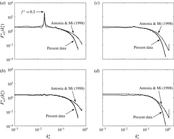
Comparison on the centreline between the present spectra (solid line) of
 $\unicode[STIX]{x1D714}_{3}$
and
 $\unicode[STIX]{x1D714}_{2}$
and those of Antonia & Mi (Reference Antonia and Mi1998) (dashed line) at (a,b)
 $x/d=10$
and (c,d)
 $x/d=40$
.

In order to confirm the above spectral attenuation estimates, the present spectra of
 $\unicode[STIX]{x1D714}_{2}$
and
 $\unicode[STIX]{x1D714}_{3}$
on the centreline at
 $x/d=10$
and 40 are compared in figure 2 with the measurements of Antonia & Mi (Reference Antonia and Mi1998) (only
 $\unicode[STIX]{x1D714}_{2}$
and
 $\unicode[STIX]{x1D714}_{3}$
were measured by these authors). The spatial resolution of their probe was better than that of the present probe. In their probe,
 $\unicode[STIX]{x0394}y~(=\unicode[STIX]{x0394}z)$
was approximately
 $6\unicode[STIX]{x1D702}$
and
 $4\unicode[STIX]{x1D702}$
at
 $x/d=10$
and 40 respectively (The corresponding present values are
 $11.2\unicode[STIX]{x1D702}$
and
 $6.4\unicode[STIX]{x1D702}$
for
 $\unicode[STIX]{x0394}y$
, and
 $15.1\unicode[STIX]{x1D702}$
and
 $8.6\unicode[STIX]{x1D702}$
for
 $\unicode[STIX]{x0394}z$
). The present spectra start to deviate from those of Antonia & Mi (Reference Antonia and Mi1998) at
 $k_{1}^{\ast }\approx 0.18(x/d=10)$
and
 $k_{1}^{\ast }\approx 0.22(x/d=40)$
. The spectral comparison of figure 2 confirms our earlier estimation that the attenuation of the present spectra occurs at wavenumbers larger than those that contribute most significantly to the mean enstrophy. Since the spatial resolution of temperature derivatives is better than that of the vorticity probe (the smallest scale of the scalar field, i.e. the Batchelor scale
 $\unicode[STIX]{x1D702}_{B}\equiv (\unicode[STIX]{x1D708}\unicode[STIX]{x1D705}^{2}/\unicode[STIX]{x1D716})^{1/4}=\unicode[STIX]{x1D702}/Pr^{1/2}$
, is slightly larger than
 $\unicode[STIX]{x1D702}$
for
 $Pr=0.7$
), it is reasonable to assume that the attenuation of the scalar derivative spectra is, at worst, comparable to that of the vorticity spectra.
3 Phase and structural averaging
3.1 Phase averaging
A phase-averaging technique is used to extract the coherent structures. The technique is an improvement over that used by Zhou, Zhang & Yiu (Reference Zhou, Zhang and Yiu2002b
) and Zhou & Yiu (Reference Zhou and Yiu2006). Briefly, the transverse velocity fluctuation signal
 $v$
, which is used as the reference phase, from the probe at each lateral measurement location is filtered using a fourth-order Butterworth filter with the centre frequency set at
 $f_{shedding}$
. A cross-correlation between the measured signal
 $v$
and the filtered signal
 $v_{f}$
is carried out to determine the average phase shift between
 $v_{f}$
and the measured
 $v$
. This shift is then applied to
 $v_{f}$
and a new reference signal
 $v_{f}^{\prime }$
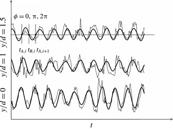
is formed. Figure 3 illustrates the
 $v$
signals at three typical lateral locations at
 $x/d=10$
and the corresponding shifted
 $v_{f}^{\prime }$
signals.
Comparison of the measured signal
 $v$
(the thin line) and the shifted filtered signal
 $v_{f}^{\prime }$
(the thicker line) at
 $x/d=10$
.

Two phases of particular interest are identified on
 $v_{f}^{\prime }$
, namely
 $$\begin{eqnarray}\displaystyle & \displaystyle \text{phase A: }v_{f}^{\prime }=0\quad \text{and}\quad \frac{\text{d}v_{f}^{\prime }}{\text{d}t}>0, & \displaystyle\end{eqnarray}$$
and
 $$\begin{eqnarray}\displaystyle & \displaystyle \text{phase B: }v_{f}^{\prime }=0\quad \text{and}\quad \frac{\text{d}v_{f}^{\prime }}{\text{d}t}<0. & \displaystyle\end{eqnarray}$$
The two phases correspond to instants
 $t_{A,i}$
and
 $t_{B,i}$
respectively. The origin of time is arbitrary. The phase of the measured fluctuation signals is then determined as
 $$\begin{eqnarray}\displaystyle & \displaystyle \unicode[STIX]{x1D719}=\unicode[STIX]{x03C0}\frac{t-t_{A,i}}{t_{B,i}-t_{A,i}},\quad t_{A,i}<t<t_{B,i} & \displaystyle\end{eqnarray}$$
and
 $$\begin{eqnarray}\displaystyle \unicode[STIX]{x1D719}=\unicode[STIX]{x03C0}\frac{t-t_{B,i}}{t_{A,i+1}-t_{B,i}}+\unicode[STIX]{x03C0},\quad t_{B,i}<t<t_{A,i+1}. & & \displaystyle\end{eqnarray}$$
The interval between phases A and B is made equal to
 $0.5T_{s}=0.5/f_{s}$
by compressing or stretching and is further divided into 20 equal intervals. The total number of detections is approximately 1980, 1700 and 1050 for
 $x/d=10,20$
and 40 respectively.
The instantaneous quantity
 $\unicode[STIX]{x1D6E4}$
may be viewed as the sum of the time-averaged component
 $\overline{\unicode[STIX]{x1D6E4}}$
and the fluctuating component
 $\unicode[STIX]{x1D6FD}$
, which can be further decomposed into a coherent fluctuation
 $\widetilde{\unicode[STIX]{x1D6FD}}$
and a remainder
 $\unicode[STIX]{x1D6FD}_{r}$
, namely
 $$\begin{eqnarray}\displaystyle & \unicode[STIX]{x1D6FD}=\widetilde{\unicode[STIX]{x1D6FD}}+\unicode[STIX]{x1D6FD}_{r}. & \displaystyle\end{eqnarray}$$
The coherent part
 $\widetilde{\unicode[STIX]{x1D6FD}}\equiv \langle \unicode[STIX]{x1D6FD}\rangle$
reflects the effect from the large-scale coherent structures, while the remainder
 $\unicode[STIX]{x1D6FD}_{r}$
reflects largely the random incoherent motions in the flow. After multiplying (3.5) by
 $\unicode[STIX]{x1D6FE}=\widetilde{\unicode[STIX]{x1D6FE}}+\unicode[STIX]{x1D6FE}_{r}$
, we obtain
 $$\begin{eqnarray}\displaystyle & \unicode[STIX]{x1D6FD}\unicode[STIX]{x1D6FE}=\widetilde{\unicode[STIX]{x1D6FD}}\widetilde{\unicode[STIX]{x1D6FE}}+\widetilde{\unicode[STIX]{x1D6FD}}\unicode[STIX]{x1D6FE}_{r}+\widetilde{\unicode[STIX]{x1D6FE}}\unicode[STIX]{x1D6FD}_{r}+\unicode[STIX]{x1D6FD}_{r}\unicode[STIX]{x1D6FE}_{r}. & \displaystyle\end{eqnarray}$$
By phase averaging (3.6) and assuming a zero correlation between coherent and remainder fluctuations, i.e.
 $\langle \widetilde{\unicode[STIX]{x1D6FD}}\unicode[STIX]{x1D6FE}_{r}\rangle =0$
and
 $\langle \widetilde{\unicode[STIX]{x1D6FE}}\unicode[STIX]{x1D6FD}_{r}\rangle =0$
, we obtain
 $$\begin{eqnarray}\langle \unicode[STIX]{x1D6FD}\unicode[STIX]{x1D6FE}\rangle =\widetilde{\unicode[STIX]{x1D6FD}}\widetilde{\unicode[STIX]{x1D6FE}}+\langle \unicode[STIX]{x1D6FD}_{r}\unicode[STIX]{x1D6FE}_{r}\rangle ,\end{eqnarray}$$
where
 $\unicode[STIX]{x1D6FD}$
and
 $\unicode[STIX]{x1D6FE}$
represent either
 $u_{i}$
,
 $\unicode[STIX]{x1D703}$
,
 $\unicode[STIX]{x1D714}_{i}$
or
 $\unicode[STIX]{x1D703}_{,i}$
.
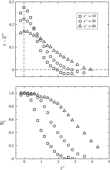
Distribution of mean streamwise velocity and temperature at
 $x^{+}=10$
, 20 and 40. Dashed lines are drawn in the mean velocity plot to mark out the positions
 $y^{+}=0$
and
 $1-\overline{U}^{+}=0$
respectively.

3.2 Structural averaging
Once the coherent components are extracted from the examined quantities, the averaged coherent contributions to the products of fluctuating components within one period can be given in terms of the structural average. The conditionally averaged structure begins at
 $n_{1}$
samples (corresponding to
 $\unicode[STIX]{x1D719}=-\unicode[STIX]{x03C0}$
) before
 $\unicode[STIX]{x1D719}=0$
and ends at
 $n_{2}$
samples (corresponding to
 $\unicode[STIX]{x1D719}=\unicode[STIX]{x03C0}$
) after
 $\unicode[STIX]{x1D719}=0$
. The structural average, denoted by a double overbar, is defined by
 $$\begin{eqnarray}\overline{\overline{\widetilde{\unicode[STIX]{x1D6FD}}\widetilde{\unicode[STIX]{x1D6FE}}}}=\frac{1}{n_{1}+n_{2}+1}\mathop{\sum }_{-n_{1}}^{n_{2}}\widetilde{\unicode[STIX]{x1D6FD}}\widetilde{\unicode[STIX]{x1D6FE}}.\end{eqnarray}$$
4 Time-averaged mean velocity and temperature
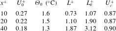
Figure 4 shows the time-averaged mean velocity defect
 $1-\overline{U}^{+}$
and temperature
 $\overline{\unicode[STIX]{x1D6E9}}^{+}$
distributions measured at
 $x^{+}=10,20$
and 40, where the ‘
 $+$
’ indicates normalization by
 $U_{1},d$
and
 $\unicode[STIX]{x1D6E9}_{0}$
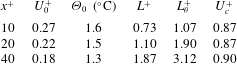
. This normalization is used only for convenience since the velocity and temperature fields in the present flow are not self-preserving. Table 2 lists the maximum mean velocity defect
 $U_{0}^{+}$
, temperature excess
 $\unicode[STIX]{x1D6E9}_{0}$
, mean velocity half-width
 $L^{+}$
and mean temperature half-width
 $L_{\unicode[STIX]{x1D703}}^{+}$
extracted from figure 4, along with the convection velocity
 $U_{c}^{+}$
of vortices, which is estimated as
 $\overline{U}+\widetilde{u}$
at the phase-averaged vortex centre, as used by Zhou & Antonia (Reference Zhou and Antonia1992). Here,
 $U_{0}^{+}$
is 0.27, 0.22 and 0.18 at
 $x^{+}=10$
, 20 and 40 respectively. These values are slightly larger than their counterparts (0.22, 0.19, 0.16) reported by Antonia & Mi (Reference Antonia and Mi1998) at
 $Re=3000$
. The non-dimensional momentum thickness
 $\unicode[STIX]{x1D6FF}_{M}/d$
(
 $\equiv \int _{-\infty }^{\infty }U/U_{1}(1-U/U_{1})\,\text{d}y$
, e.g. Tennekes & Lumley Reference Tennekes and Lumley1972) at
 $x^{+}=40$
is 0.49, which is quite close to that estimated by Antonia & Rajagopalan (Reference Antonia and Rajagopalan1990), approximately 0.45 at
 $Re=5600$
. The spanwise vortices decay downstream. So does their ability to retain heat (e.g. Matsumura & Antonia Reference Matsumura and Antonia1993). As a result,
 $\unicode[STIX]{x1D6E9}_{0}$
diminishes. The mean velocity half-width
 $L^{+}$
is smaller than
 $L_{\unicode[STIX]{x1D703}}^{+}$
, suggesting a more efficient transport of heat than momentum. The ratio
 $L^{+}/L_{\unicode[STIX]{x1D703}}^{+}$
is 0.68, 0.58 and 0.60 at
 $x^{+}=10,20$
and 40 respectively, in reasonable agreement with their counterparts (0.76, 0.56, 0.56) reported by Zhou et al. (Reference Zhou, Zhang and Yiu2002b
) at
 $Re=5800$
.
Maximum mean velocity defect, mean temperature excess, mean velocity half-width, mean temperature half-width and vortex convection velocity.
5 Similarity between scalar dissipation rate and enstrophy
5.1 Spectral similarity between enstrophy and scalar dissipation rate
Corrsin (Reference Corrsin1953) was the first to point out the similarity between the transport equations for the mean enstrophy
 $\overline{\unicode[STIX]{x1D714}_{i}\unicode[STIX]{x1D714}_{i}}$
and the mean scalar dissipation rate
 $\overline{\unicode[STIX]{x1D703}_{,i}\,\unicode[STIX]{x1D703}_{,i}}$
, which underpins a possible similarity between
 $\overline{\unicode[STIX]{x1D714}_{i}\unicode[STIX]{x1D714}_{i}}$
and
 $\overline{\unicode[STIX]{x1D703}_{,i}\,\unicode[STIX]{x1D703}_{,i}}$
in either spectral or physical space. The similarity in spectral space is examined in this section, while the similarity in physical space will be considered in the next section.
The power spectrum density function of a quantity
 $\unicode[STIX]{x1D6FC}$
is defined such that
 $\int _{0}^{\infty }E_{\unicode[STIX]{x1D6FC}}(k)\,\text{d}k=\overline{\unicode[STIX]{x1D6FC}^{2}}$
, i.e. the area under the curve
 $E_{\unicode[STIX]{x1D6FC}}(k)$
represents the variance
 $\overline{\unicode[STIX]{x1D6FC}^{2}}$
. It should be noted that
 $kE_{\unicode[STIX]{x1D6FC}}(k)$
is plotted using a linear scale along the ordinate and log
 $k$
along the abscissa so that the area under the curve is still proportional to
 $\overline{\unicode[STIX]{x1D6FC}^{2}}$
, and thus the wavenumber corresponding to the peak of the spectrum is related to the most energetic scale. Following Fulachier & Dumas (Reference Fulachier and Dumas1976), Fulachier & Antonia (Reference Fulachier and Antonia1984) and Antonia et al. (Reference Antonia, Abe and Kawamura2009), we use the normalized spectra such that
 $\int _{0}^{\infty }F_{\unicode[STIX]{x1D6FC}}(k)\,\text{d}k=\int _{0}^{\infty }E_{\unicode[STIX]{x1D6FC}}(k)/\overline{\unicode[STIX]{x1D6FC}^{2}}\,\text{d}k=1$
.
The spectra of
 $\overline{\unicode[STIX]{x1D714}_{i}\unicode[STIX]{x1D714}_{i}}$
and
 $\overline{\unicode[STIX]{x1D703}_{,i}\,\unicode[STIX]{x1D703}_{,i}}$
are defined as
 $$\begin{eqnarray}F_{\unicode[STIX]{x1D714}}=(\overline{\unicode[STIX]{x1D714}_{1}\unicode[STIX]{x1D714}_{1}}/\overline{\unicode[STIX]{x1D714}_{i}\unicode[STIX]{x1D714}_{i}})F_{\unicode[STIX]{x1D714}_{1}}+(\overline{\unicode[STIX]{x1D714}_{2}\unicode[STIX]{x1D714}_{2}}/\overline{\unicode[STIX]{x1D714}_{i}\unicode[STIX]{x1D714}_{i}})F_{\unicode[STIX]{x1D714}_{2}}+(\overline{\unicode[STIX]{x1D714}_{3}\unicode[STIX]{x1D714}_{3}}/\overline{\unicode[STIX]{x1D714}_{i}\unicode[STIX]{x1D714}_{i}})F_{\unicode[STIX]{x1D714}_{3}}\end{eqnarray}$$
and
 $$\begin{eqnarray}F_{\unicode[STIX]{x1D712}}=(\overline{\unicode[STIX]{x1D703}_{,1}\unicode[STIX]{x1D703}_{,1}}/\overline{\unicode[STIX]{x1D703}_{,i}\,\unicode[STIX]{x1D703}_{,i}})F_{\unicode[STIX]{x1D703},1}+(\overline{\unicode[STIX]{x1D703}_{,2}\unicode[STIX]{x1D703}_{,2}}/\overline{\unicode[STIX]{x1D703}_{,i}\,\unicode[STIX]{x1D703}_{,i}})F_{\unicode[STIX]{x1D703},2}+(\overline{\unicode[STIX]{x1D703}_{,3}\unicode[STIX]{x1D703}_{,3}}/\overline{\unicode[STIX]{x1D703}_{,i}\,\unicode[STIX]{x1D703}_{,i}})F_{\unicode[STIX]{x1D703},3},\end{eqnarray}$$
where
 $F_{\unicode[STIX]{x1D714}i}$
and
 $F_{\unicode[STIX]{x1D703},i}$
are the power spectral density functions of the
 $i$
components of
 $\overline{\unicode[STIX]{x1D714}_{i}\unicode[STIX]{x1D714}_{i}}$
and
 $\overline{\unicode[STIX]{x1D703}_{,i}\,\unicode[STIX]{x1D703}_{,i}}$
respectively, and are normalized to a unity integral, i.e.
 $\int _{0}^{\infty }F_{\unicode[STIX]{x1D714}i}\,\text{d}k_{1}^{\ast }=1$
and
 $\int _{0}^{\infty }F_{\unicode[STIX]{x1D703},i}\,\text{d}k_{1}^{\ast }=1$
.
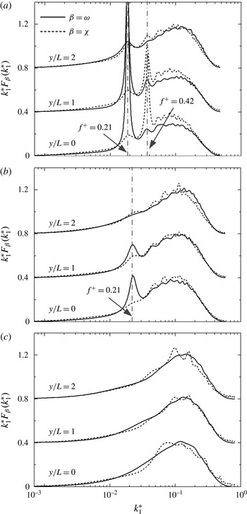
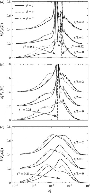
The distributions of
 $k_{1}^{\ast }F_{\unicode[STIX]{x1D714}}$
and
 $k_{1}^{\ast }F_{\unicode[STIX]{x1D712}}$
(figure 5) follow each other closely at all three typical transverse positions, i.e.
 $y/L=0$
, 1 and 2, especially at
 $x^{+}=20$
and 40. The departures at small wavenumbers, particularly evident at
 $x^{+}=10$
and 20, are related to the organized Kármán vortices that occur at the Strouhal number
 $St=0.21$
. At
 $x^{+}=10$
,
 $F_{\unicode[STIX]{x1D714}}$
displays a pronounced peak at
 $f^{+}~(\equiv fU_{1}/d)=St$
. However, the most pronounced peak in
 $F_{\unicode[STIX]{x1D712}}$
occurs at a wavenumber corresponding to
 $f^{+}=2St$
. It will be shown and discussed later that the
 $\widetilde{\unicode[STIX]{x1D703}}_{,i}^{+}\widetilde{\unicode[STIX]{x1D703}}_{,i}^{+}$
contours are characterized by twin peaks caused by the entrainment of cold fluid into the heated wake from both sides of the free stream. As a result, the predominant frequency of
 $F_{\unicode[STIX]{x1D712}}$
is twice that of
 $F_{\unicode[STIX]{x1D714}}$
. At
 $x^{+}=20$
, a peak is still evident at
 $f^{+}=St$
for
 $F_{\unicode[STIX]{x1D714}}$
when
 $y/L\leqslant 1$
, although it is much less pronounced than at
 $x^{+}=10$
. However, the peak at
 $f^{+}=2St$
is hardly discernible in
 $F_{\unicode[STIX]{x1D712}}$
at
 $f^{+}=2St$
. By
 $x^{+}=40$
, the peaks
 $f^{+}=0.21$
or 0.42 have virtually disappeared in both
 $F_{\unicode[STIX]{x1D712}}$
and
 $F_{\unicode[STIX]{x1D714}}$
, and the two spectra follow each other more closely than at
 $x^{+}=10$
or 20. The streamwise evolution of the spectra at low wavenumbers suggests that the contribution from the coherent structures to
 $\overline{\unicode[STIX]{x1D703}_{,i}\,\unicode[STIX]{x1D703}_{,i}}$
and
 $\overline{\unicode[STIX]{x1D714}_{i}\unicode[STIX]{x1D714}_{i}}$
plays a crucial role in degrading the spectral similarity. This is, in fact, substantiated by
 $F_{\unicode[STIX]{x1D712}}$
and
 $F_{\unicode[STIX]{x1D714}}$
at
 $y/L=2$
, where the coherent motion is rather weak and there is no evident peak at either
 $f^{+}=0.21$
or 0.42 even for
 $x^{+}=10$
and 20. As such,
 $F_{\unicode[STIX]{x1D712}}$
and
 $F_{\unicode[STIX]{x1D714}}$
follow each other well at low wavenumbers.
Spectral density functions, multiplied by
 $k_{1}^{\ast }$
, of
 $\unicode[STIX]{x1D714}$
and
 $\unicode[STIX]{x1D712}$
measured at
 $y/L=0$
, 1 and 2, where
 $L$
is the wake half-width: (a)
 $x^{+}=10$
, (b) 20, (c) 40. It should be noted that the origins for the spectra at
 $y/L=1$
and 2 are shifted by 0.4 and 0.8 for the ordinate respectively.

The similarity between
 $F_{\unicode[STIX]{x1D712}}$
and
 $F_{\unicode[STIX]{x1D714}}$
is more tenable at
 $y/L=1$
than at
 $y/L=0$
or 2 over the high-wavenumber range. This is especially evident at
 $x^{+}=20$
and 40. Antonia et al. (Reference Antonia, Abe and Kawamura2009) found that in the outer region of a channel flow the spectral similarity between
 $\overline{\unicode[STIX]{x1D703}_{,i}\,\unicode[STIX]{x1D703}_{,i}}$
and
 $\overline{\unicode[STIX]{x1D714}_{i}\unicode[STIX]{x1D714}_{i}}$
is not as good as near the wall due to the higher mean velocity and temperature gradients in this region. This improved similarity at
 $y/L=1$
(figure 5
b–c) suggests that the higher mean shear at
 $y/L=1$
may act to promote the similarity between
 $F_{\unicode[STIX]{x1D712}}$
and
 $F_{\unicode[STIX]{x1D714}}$
. This effect is more evident at high wavenumbers since the influence of the coherent motion may overwhelm that due to
 $\unicode[STIX]{x2202}\overline{U}/\unicode[STIX]{x2202}y$
and
 $\unicode[STIX]{x2202}\overline{\unicode[STIX]{x1D6E9}}/\unicode[STIX]{x2202}y$
at low wavenumbers. One way of quantifying the similarity between spectra is to calculate the ratio of the two spectra. For wavenumbers that contribute most to
 $\overline{\unicode[STIX]{x1D703}_{,i}\,\unicode[STIX]{x1D703}_{,i}}$
and
 $\overline{\unicode[STIX]{x1D714}_{i}\unicode[STIX]{x1D714}_{i}}$
,
 $F_{\unicode[STIX]{x1D712}}/F_{\unicode[STIX]{x1D714}}$
is approximately 1 within an error of approximately
 $\pm 10\,\%$
at
 $y/L=1$
at
 $x^{+}=20$
and 40.
Spectral density functions, multiplied by
 $k_{1}^{\ast }$
, of
 $\unicode[STIX]{x1D712},\unicode[STIX]{x1D714}$
, and their components at
 $y/L=1$
: (a,d)
 $x^{+}=10$
, (b,e)
 $x^{+}=20$
, (c,f)
 $x^{+}=40$
.

Probability density function of
 $\cos (\unicode[STIX]{x1D719})$
, where
 $\unicode[STIX]{x1D719}$
is the angle between the vorticity vector
 $\unicode[STIX]{x1D74E}$
and the scalar gradient vector
 $\unicode[STIX]{x1D735}\unicode[STIX]{x1D703}$
, and
 $\cos (\unicode[STIX]{x1D719})=\unicode[STIX]{x1D74E}\boldsymbol{\cdot }\unicode[STIX]{x1D735}\unicode[STIX]{x1D703}/(|\unicode[STIX]{x1D74E}||\unicode[STIX]{x1D735}\unicode[STIX]{x1D703}|)$
: (a)
 $x^{+}=10$
, (b)
 $x^{+}=20$
, (c)
 $x^{+}=40$
.

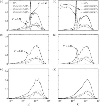
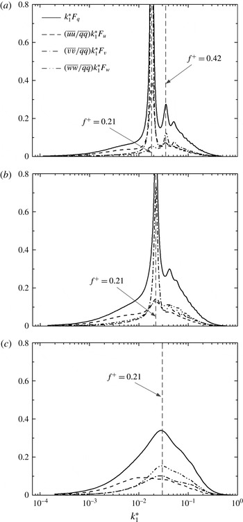
Figure 6 presents the spectra of the scalar dissipation rate, the enstrophy and their components. The peak at
 $f^{+}=St$
in
 $F_{\unicode[STIX]{x1D714}}$
results mainly from the contribution of the spanwise vorticity component, i.e. from
 $F_{\unicode[STIX]{x1D714}3}$
, while that at
 $f^{+}=0.42$
in
 $F_{\unicode[STIX]{x1D712}}$
is mostly contributed by
 $F_{\unicode[STIX]{x1D703},1}$
. Since none of the components of
 $F_{\unicode[STIX]{x1D712}}$
or
 $F_{\unicode[STIX]{x1D714}}$
can be neglected, the spectral similarity is a reflection of the summation of all three components. There is a difference between the contribution of
 $F_{\unicode[STIX]{x1D703},i}$
to
 $F_{\unicode[STIX]{x1D712}}$
and that of
 $F_{\unicode[STIX]{x1D714}_{i}}$
to
 $F_{\unicode[STIX]{x1D714}}$
. The most energetic wavenumbers, excluding the most pronounced peak, of
 $F_{\unicode[STIX]{x1D703},2}$
and
 $F_{\unicode[STIX]{x1D703},3}$
are comparable but lower than those of
 $F_{\unicode[STIX]{x1D703},1}$
; however, the most energetic wavenumbers of
 $F_{\unicode[STIX]{x1D714}2}$
and
 $F_{\unicode[STIX]{x1D714}3}$
are higher than those of
 $F_{\unicode[STIX]{x1D714}1}$
. The difference is especially evident at
 $x^{+}=40$
. Antonia et al. (Reference Antonia, Abe and Kawamura2009) made a similar observation in the outer region of a turbulent channel flow and suggested that this difference in the occurrence of the most energetic wavenumbers between
 $F_{\unicode[STIX]{x1D714}_{i}}$
and
 $F_{\unicode[STIX]{x1D703}_{,i}}$
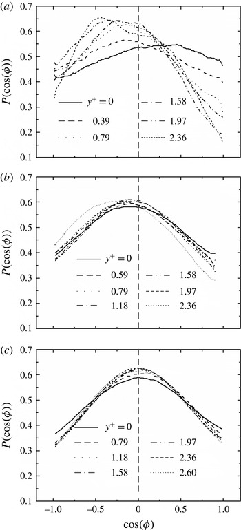
is linked to the different structures between the scalar dissipation rate and the enstrophy, i.e. the tubular structures in the enstrophy field and the sheet-like structures in the scalar dissipation rate field. The same explanation applies here. The presence of sheet-like structures in this flow is corroborated by the probability density function (p.d.f.) of
 $\cos (\unicode[STIX]{x1D719})~(=\unicode[STIX]{x1D74E}\boldsymbol{\cdot }\unicode[STIX]{x1D735}\unicode[STIX]{x1D703}/(|\unicode[STIX]{x1D74E}||\unicode[STIX]{x1D735}\unicode[STIX]{x1D703}|))$
(figure 7). In the presence of sheet-like structures in
 $\unicode[STIX]{x1D712}$
, the vorticity and scalar gradient vectors tend to be aligned with the directions of the intermediate and compressive principal rates of strain respectively (Abe & Antonia Reference Abe and Antonia2009; Antonia et al.
Reference Antonia, Abe and Kawamura2009). Then, one may expect that
 $\unicode[STIX]{x1D74E}$
and
 $\unicode[STIX]{x1D735}\unicode[STIX]{x1D703}$
should be statistically orthogonal to each other, as is shown in figure 7(b,c), where the peaks in the p.d.f.s of
 $\cos (\unicode[STIX]{x1D719})$
occur almost at
 $\cos (\unicode[STIX]{x1D719})=0$
for
 $x^{+}=20$
and 40. The p.d.f. of
 $\cos (\unicode[STIX]{x1D719})$
displays significant scatter at
 $x^{+}=10$
across the wake, suggesting that the scalar at this location does not yet feel the strain associated with the velocity field. This is not surprising since heat is mostly contained within the Kármán vortex rollers at
 $x^{+}=10$
, as observed by Matsumura & Antonia (Reference Matsumura and Antonia1993) and confirmed by the present phase-averaged data (figure 8
a), while the maximum strain rate occurs near the saddle points along the divergent separatrix (Hussain & Hayakawa Reference Hussain and Hayakawa1987; Thiesset, Danaila & Antonia Reference Thiesset, Danaila and Antonia2013). This is also internally consistent with the earlier observations from the spectra; that is, the mean shear has little effect in promoting the similarity between
 $F_{\unicode[STIX]{x1D714}}$
and
 $F_{\unicode[STIX]{x1D712}}$
at
 $x^{+}=10$
, and the departure between
 $F_{\unicode[STIX]{x1D712}}$
and
 $F_{\unicode[STIX]{x1D714}}$
is larger at
 $x^{+}=10$
than
 $x^{+}=20$
or 40. Evidently, when the passive scalar is more stretched due to the rate of strain at
 $x^{+}=40$
,
 $\unicode[STIX]{x1D714}$
and
 $\unicode[STIX]{x1D735}\unicode[STIX]{x1D703}$
are statistically orthogonal to each other (figure 7
c) and the similarity between
 $F_{\unicode[STIX]{x1D714}}$
and
 $F_{\unicode[STIX]{x1D712}}$
is also best (figure 5
c). Observation indicates that the more the passive scalar is stretched, or more effectively mixed by the rate of strain, the better the similarity between
 $F_{\unicode[STIX]{x1D714}}$
and
 $F_{\unicode[STIX]{x1D712}}$
will be.
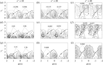
Isocontours of phase-averaged (a–c) coherent temperature (contour intervals
 $=0.089$
, 0.018, 0.020), (d–f) scalar dissipation rate (0.18, 0.010, 0.004) and (g–i) enstrophy (0.11, 0.043, 0.005). Hereafter,
 $+$
indicates centres of vortices and
 $\times$
indicates saddle points. The thicker dashed lines denote the periphery of the coherent spanwise vorticity
 $\widetilde{\unicode[STIX]{x1D714}}_{z}^{+}$
. The dash-dotted line through the saddle point represents the diverging separatrix. The flow is from left to right.

5.2 Phase-averaged scalar dissipation rate and enstrophy
5.2.1 Coherent scalar dissipation rate and enstrophy
The intermediate wake is associated with strong anisotropic coherent structures, in distinct contrast to the weak large-scale coherent structures in the far wake. Significant physical insight may be gained by understanding the topological features of the structures associated with the enstrophy and scalar dissipation rate. To this end, the isocontours of their phase-averaged quantities and remainders (§ 3) will be examined and discussed, along with their contributions to the Reynolds-averaged quantities. Hereafter, in all of the isocontour figures, the phase
 $\unicode[STIX]{x1D719}$
in the range
 $-2\unicode[STIX]{x03C0}$
to
 $2\unicode[STIX]{x03C0}$
will be interpreted in terms of a longitudinal distance, with
 $\unicode[STIX]{x1D719}=2\unicode[STIX]{x03C0}$
corresponding to the averaged vortex wavelength. The same scale is used for the longitudinal and lateral directions in the contour plots in an effort to minimize any possible distortion in the physical space. The symbols ‘
 $+$
’ and ‘
 $\times$
’ denote the centres and saddle points respectively. The thick dashed lines give an approximate idea of the periphery of the spanwise vortex, defined rather arbitrarily by a contour level corresponding to approximately 25 % of the maximum value of
 $\widetilde{\unicode[STIX]{x1D714}}_{z}^{+}$
. The dash-dotted line through the saddle point represents the diverging separatrix.
The isocontours of
 $\widetilde{\unicode[STIX]{x1D703}}_{,i}^{+}\widetilde{\unicode[STIX]{x1D703}}_{,i}^{+}$
and
 $\widetilde{\unicode[STIX]{x1D714}}_{i}^{+}\widetilde{\unicode[STIX]{x1D714}}_{i}^{+}$
(figure 8
d–i) exhibit a significant difference from each other, conforming to the departures at the low wavenumbers in
 $F_{\unicode[STIX]{x1D714}}$
and
 $F_{\unicode[STIX]{x1D712}}$
. Two concentrations of
 $\widetilde{\unicode[STIX]{x1D703}}_{,i}^{+}\widetilde{\unicode[STIX]{x1D703}}_{,i}^{+}$
occur about each vortex centre, evident at
 $x^{+}=10$
and 20 (figure 8
d,e), originating from the temperature gradients between the free-stream cold fluid engulfed by the coherent motion and the warm fluid in the central region of the wake. Specifically, as may be inferred from the
 $\widetilde{\unicode[STIX]{x1D703}}^{+}$
contours (figure 8
a–c), the downstream concentration within one structure results from an interaction between the warm fluid in the wake and the cold fluid engulfed from the free stream on the same side of the vortex, while the upstream concentration is due to an interaction between the warm fluid in the wake and the cold fluid from the free stream on the other side of the vortex. In contrast, the concentration of
 $\widetilde{\unicode[STIX]{x1D714}}_{i}^{+}\widetilde{\unicode[STIX]{x1D714}}_{i}^{+}$
(figure 8
g–i) is closely linked to the vortex, and thus its contours resemble those of the coherent spanwise vorticity (cf. figure 11 in Zhou, Zhou & Yiu Reference Zhou, Zhou, Yiu and Chua2003) and the maximum coincides with the vortex centre. These differences between the coherent structures of the scalar dissipation rate and the enstrophy underpin our earlier assertion that it is the coherent motion of the flow that degrades the similarity between
 $F_{\unicode[STIX]{x1D714}}$
and
 $F_{\unicode[STIX]{x1D712}}$
at low wavenumbers. It should be noted that some elongated sheet-like structures of
 $\widetilde{\unicode[STIX]{x1D703}}_{,i}^{+}\widetilde{\unicode[STIX]{x1D703}}_{,i}^{+}$
occur along the divergent separatrix at
 $x^{+}=20$
and 40 (figure 8
e,f) but not at
 $x^{+}=10$
(figure 8
d), corroborating our suggestion, based on figure 7, that the scalar is not yet fully stretched at
 $x^{+}=10$
by the strain rate imposed by the velocity field, and the presence of sheet-like structures is not evident until
 $x^{+}=20$
.
5.2.2 Incoherent scalar dissipation rate and enstrophy
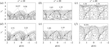
The contours of the remainders
 $\langle \unicode[STIX]{x1D703}_{r,i}^{+}\unicode[STIX]{x1D703}_{r,i}^{+}\rangle$
and
 $\langle \unicode[STIX]{x1D714}_{ri}^{+}\unicode[STIX]{x1D714}_{ri}^{+}\rangle$
(figure 9) are closely similar to each other, in distinct contrast to the difference between
 $\widetilde{\unicode[STIX]{x1D703}}_{,i}^{+}\widetilde{\unicode[STIX]{x1D703}}_{,i}^{+}$
and
 $\widetilde{\unicode[STIX]{x1D714}}_{i}^{+}\widetilde{\unicode[STIX]{x1D714}}_{i}^{+}$
. At
 $x^{+}=10$
and 20, the concentrations of
 $\langle \unicode[STIX]{x1D703}_{r,i}^{+}\unicode[STIX]{x1D703}_{r,i}^{+}\rangle$
and
 $\langle \unicode[STIX]{x1D714}_{ri}^{+}\unicode[STIX]{x1D714}_{ri}^{+}\rangle$
occur mostly within the spanwise vortex, and their maxima almost coincide with the vortex centre. The result is consistent with the observation that the maximum incoherent turbulent intensity coincides with the spanwise vortex centre (Hussain & Hayakawa Reference Hussain and Hayakawa1987), and the scalar dissipation process is highly correlated with the turbulent motions or small-scale vorticity (Warhaft Reference Warhaft2000). The similar behaviour between
 $\langle \unicode[STIX]{x1D703}_{r,i}^{+}\unicode[STIX]{x1D703}_{r,i}^{+}\rangle$
and
 $\langle \unicode[STIX]{x1D714}_{ri}^{+}\unicode[STIX]{x1D714}_{ri}^{+}\rangle$
provides an explanation for the relatively good similarity between
 $F_{\unicode[STIX]{x1D712}}$
and
 $F_{\unicode[STIX]{x1D714}}$
at the high wavenumbers (figure 5). It should be noted that the similarity between
 $\langle \unicode[STIX]{x1D703}_{r,i}^{+}\unicode[STIX]{x1D703}_{r,i}^{+}\rangle$
and
 $\langle \unicode[STIX]{x1D714}_{ri}^{+}\unicode[STIX]{x1D714}_{ri}^{+}\rangle$
deteriorates at
 $x^{+}=40$
since heat has been transported out of the spanwise vortex, as indicated by the
 $\widetilde{\unicode[STIX]{x1D703}}^{+}$
contours (figure 8
a–c), and consequently the maximum of
 $\langle \unicode[STIX]{x1D703}_{r,i}^{+}\unicode[STIX]{x1D703}_{r,i}^{+}\rangle$
moves away from the vortex centre towards the free stream.
Isocontours of the remainder of (a–c) the scalar dissipation rate (contour intervals
 $=0.68$
, 0.09, 0.15) and (d–f) the enstrophy (0.25, 0.09, 0.029).

Averaged contributions from the coherent structures to the mean enstrophy and the mean scalar dissipation rate. The percentages are all calculated based the values of the corresponding
 $S_{c}$
and
 $S_{g}$
before they are rounded.

5.2.3 Coherent contribution to the scalar dissipation rate and enstrophy
The contributions from the coherent motion to the Reynolds-averaged quantities may be quantified by comparing the Reynolds and structural averages of
 $\unicode[STIX]{x1D703}_{,i}^{+}\unicode[STIX]{x1D703}_{,i}^{+}$
and
 $\unicode[STIX]{x1D714}_{i}^{+}\unicode[STIX]{x1D714}_{i}^{+}$
. In order to quantify the coherent contribution to the scalar dissipation rate and enstrophy across the wake, we follow Matsumura & Antonia (Reference Matsumura and Antonia1993) and define the coherent contribution to the Reynolds-averaged quantity as
 $$\begin{eqnarray}\unicode[STIX]{x1D6FC}=S_{c}/S_{g},\end{eqnarray}$$
where
 $S_{c}=\int _{0}^{y}|\overline{\overline{\widetilde{\unicode[STIX]{x1D6FD}}\widetilde{\unicode[STIX]{x1D6FE}}}}|\,\text{d}y$
,
 $S_{g}=\int _{0}^{Y}|\overline{\unicode[STIX]{x1D6FD}\unicode[STIX]{x1D6FE}}|\,\text{d}y$
and
 $Y$
is the position at which
 $|\overline{\unicode[STIX]{x1D6FD}\unicode[STIX]{x1D6FE}}|$
is nearly zero. The following observations can be made from the values of
 $\unicode[STIX]{x1D6FC}$
in table 3. First, the coherent contribution to the scalar dissipation rate is smaller than that to the enstrophy, regardless of
 $x^{+}$
, and decreases more rapidly with increasing
 $x^{+}$
. From
 $x^{+}=10$
to 40, the value of
 $\unicode[STIX]{x1D6FC}$
drops by a factor of 2.4 for
 $\overline{\unicode[STIX]{x1D714}_{i}^{+}\unicode[STIX]{x1D714}_{i}^{+}}$
but 11 for
 $\overline{\unicode[STIX]{x1D703}_{,i}^{+}\unicode[STIX]{x1D703}_{,i}^{+}}$
, suggesting that the structures of the temperature dissipation rate break up into small scales more rapidly downstream than the enstrophy. Second, the coherent contributions to
 $\overline{\unicode[STIX]{x1D714}_{i}^{+}\unicode[STIX]{x1D714}_{i}^{+}}$
and
 $\overline{\unicode[STIX]{x1D703}_{,i}^{+}\unicode[STIX]{x1D703}_{,i}^{+}}$
never exceed 20 %, irrespective of
 $x^{+}$
, implying that both the scalar dissipation rate and the enstrophy reside mostly in small-scale turbulent structures.
It is worth pointing out that a close correspondence between spectra does not necessarily mean a large correlation coefficient. Despite a good similarity between
 $F_{\unicode[STIX]{x1D712}}$
and
 $F_{\unicode[STIX]{x1D714}}$
(figure 5), the correlation coefficients between vorticity components (
 $\unicode[STIX]{x1D714}_{i}$
) and temperature derivatives (
 $\unicode[STIX]{x1D703}_{,i}$
) are generally quite small, with a maximum magnitude of
 $-0.2$
between
 $\unicode[STIX]{x1D714}_{z}$
and
 $\unicode[STIX]{x1D703}_{,1}$
at
 $x/d=10$
. This is mainly because the correlation between
 $u_{i}$
and
 $\unicode[STIX]{x1D703}$
in the present flow is not as good as that, for example, in the flow near a wall, where the almost perfect correspondence between thermal streaks (
 $\unicode[STIX]{x1D703}$
) and velocity streaks (
 $u_{1}$
) results in a correlation coefficient of almost 1 between
 $\unicode[STIX]{x1D714}_{z}\,({\approx}-u_{1,2})$
and
 $\unicode[STIX]{x1D703}_{,2}$
or
 $\unicode[STIX]{x1D714}_{y}\,({\approx}u_{1,3})$
and
 $\unicode[STIX]{x1D703}_{,3}$
(Abe et al.
Reference Abe, Antonia and Kawamura2009). In fact, the phase-averaged
 $\unicode[STIX]{x1D703}$
-contours show that the
 $\unicode[STIX]{x1D703}$
concentration lies mostly within the Kármán vortex, at least for
 $x^{+}=10$
and 20 (figure 8
a,b), which is consistent with the observation of Mi & Antonia (Reference Mi and Antonia1994) that the theoretical distributions of vorticity and temperature are almost identical in a diffusing line vortex. This is why the correlation coefficient between
 $\unicode[STIX]{x1D703}$
and
 $\unicode[STIX]{x1D714}_{z}$
is larger, approximately
 $-0.3$
to
 $0.4$
at
 $x^{+}=10$
and 20, than that between
 $\unicode[STIX]{x1D714}_{i}$
and
 $\unicode[STIX]{x1D703}_{,i}$
, even though the correlation coefficient between
 $\unicode[STIX]{x1D703}$
and
 $\unicode[STIX]{x1D714}_{z}$
could be underestimated since the entrained cold fluid (
 $\unicode[STIX]{x1D703}<0$
; see the dashed-line contours in figure 8
a–c) can act to partially cancel or reduce the correlation coefficient.
6 Similarity between turbulent kinetic energy and temperature variance
6.1 Spectral similarity
The similarity between turbulent kinetic energy and temperature variance is explored in both the spectral and phase-averaged physical domains. The spectrum of
 $q$
is defined following Fulachier & Dumas (Reference Fulachier and Dumas1976), Fulachier & Antonia (Reference Fulachier and Antonia1984) and Antonia et al. (Reference Antonia, Abe and Kawamura2009), namely
 $$\begin{eqnarray}F_{q}=\overline{u^{2}}/\overline{q^{2}}F_{u}+\overline{v^{2}}/\overline{q^{2}}F_{v}+\overline{w^{2}}/\overline{q^{2}}F_{w},\end{eqnarray}$$
where
 $q^{2}=u^{2}+v^{2}+w^{2}$
is the turbulent kinetic energy, and
 $F_{u},F_{v}$
and
 $F_{w}$
are the power spectral density functions of
 $u$
,
 $v$
and
 $w$
respectively, which are normalized so that
 $\int _{0}^{\infty }F_{u_{i}}\,\text{d}k_{1}^{\ast }=1$
. Fulachier & Antonia (Reference Fulachier and Antonia1984) studied the similarity between
 $F_{q}$
and
 $F_{\unicode[STIX]{x1D703}}$
in a turbulent far wake, where a comparison between
 $F_{u}$
and
 $F_{\unicode[STIX]{x1D703}}$
was also included as a reference. The similarity between
 $F_{q}$
and
 $F_{\unicode[STIX]{x1D703}}$
in the far wake is better than that between
 $F_{u}$
and
 $F_{\unicode[STIX]{x1D703}}$
. We also include
 $F_{u}$
in order to allow a comparison between the present results in the intermediate wake and the results in the far wake.
Figure 10 shows distributions of
 $k_{1}^{\ast }F_{q}$
,
 $k_{1}^{\ast }F_{u}$
and
 $k_{1}^{\ast }F_{\unicode[STIX]{x1D703}}$
at
 $y/L=0,1$
and 2 for
 $x^{+}=10$
, 20 and 40. A pronounced peak occurs at a wavenumber close to
 $St=0.21$
in all of the spectra for
 $x^{+}\leqslant 20$
. At
 $x^{+}=40$
, as the Kármán vortices break up, the peaks corresponding to
 $St=0.21$
almost disappear in
 $k_{1}^{\ast }F_{u}$
and
 $k_{1}^{\ast }F_{\unicode[STIX]{x1D703}}$
but are discernible in
 $k_{1}^{\ast }F_{q}$
, which is largely due to the contribution from
 $k_{1}^{\ast }F_{v}$
. It should be noted that a rather pronounced peak occurs at a wavenumber corresponding to
 $f^{+}=2St=0.42$
in
 $k_{1}^{\ast }F_{\unicode[STIX]{x1D703}}$
at
 $x^{+}=10$
. This is because heat is associated with both positive and negative vortices, which occur alternately near the centreline (figure 8
a–c). When advected downstream, the vortices move away from the centreline; the peak at
 $f^{+}=0.42$
is weak at
 $x^{+}=20$
and cannot be detected at
 $x^{+}=40$
.
Spectral density functions, multiplied by
 $k_{1}^{\ast }$
, of
 $\boldsymbol{q}$
,
 $u$
and
 $\unicode[STIX]{x1D703}$
measured at
 $y/L=0$
, 1, and 2: (a)
 $x^{+}=10$
, (b)
 $x^{+}=20$
, (c)
 $x^{+}=40$
.

It should be noted that the comparison between
 $k_{1}^{\ast }F_{\unicode[STIX]{x1D703}}$
and
 $k_{1}^{\ast }F_{q}$
is not particularly good, with
 $k_{1}^{\ast }F_{\unicode[STIX]{x1D703}}$
following
 $k_{1}^{\ast }F_{u}$
more closely than
 $k_{1}^{\ast }F_{q}$
almost everywhere, except near
 $y/L=2$
at
 $x^{+}=10$
and 20. Further,
 $k_{1}^{\ast }F_{\unicode[STIX]{x1D703}}$
exhibits a closer similarity to
 $k_{1}^{\ast }F_{u}$
at
 $y/L=1$
than at
 $y/L=0$
, independently of
 $x^{+}$
, due to the larger mean gradients of both velocity and temperature near
 $y/L=1$
. Observation suggests that the mean shear acts to enhance the spectral similarity between
 $k_{1}^{\ast }F_{\unicode[STIX]{x1D703}}$
and
 $k_{1}^{\ast }F_{u}$
. The mean shear, however, does not affect to a significant extent the similarity between
 $k_{1}^{\ast }F_{\unicode[STIX]{x1D703}}$
and
 $k_{1}^{\ast }F_{q}$
. As
 $x^{+}$
increases from 10 to 40, the difference between
 $k_{1}^{\ast }F_{\unicode[STIX]{x1D703}}$
and
 $k_{1}^{\ast }F_{u}$
diminishes over almost the entire range of wavenumbers, especially near
 $k^{+}$
corresponding to
 $f^{+}=0.42$
; on the other hand, the difference between
 $k_{1}^{\ast }F_{\unicode[STIX]{x1D703}}$
and
 $k_{1}^{\ast }F_{q}$
grows at high wavenumbers. In figure 11, we plot the spectra of
 $q$
at the three
 $x^{+}$
positions together with the weighted spectra of
 $u$
,
 $v$
and
 $w$
. At
 $x^{+}=10$
and 20, both
 $F_{u}$
and
 $F_{v}$
show a pronounced peak at or near
 $St=0.21$
. As
 $x^{+}$
reaches 40, the peak in
 $F_{u}$
retreats, as observed in the far wake (Fulachier & Antonia Reference Fulachier and Antonia1984). The peak of
 $F_{v}$
(also
 $F_{w}$
) remains at
 $St=0.21$
. As a result, the spectra of
 $q$
show a peak at
 $St=0.21$
(figure 10
a–c) (It should be noted that the value of
 $k_{1}^{\ast }$
corresponding to
 $St=0.21$
for all spectra increases from
 $x^{+}=10$
to 40, due to the normalization of the wavenumber (
 $k_{1}^{\ast }=2\unicode[STIX]{x03C0}f/U_{1}\unicode[STIX]{x1D702}$
), where
 $\unicode[STIX]{x1D702}$
increases for larger
 $x^{+}$
.) The similarity between
 $F_{\unicode[STIX]{x1D703}}$
and
 $F_{u}$
indicates that the scalar variance in this flow is dictated by
 $u$
, which is different from the far wake, where the velocity vector dictates the behaviour of the scalar fluctuation (Fulachier & Antonia Reference Fulachier and Antonia1984).
6.2 Coherent turbulent kinetic energy and temperature variance, and remainders
Figure 12 displays the coherent turbulent kinetic energy
 $\widetilde{q}^{+2}$
, streamwise velocity fluctuation variance
 $\widetilde{u}^{+2}$
and temperature variance
 $\widetilde{\unicode[STIX]{x1D703}}^{+2}$
at
 $x^{+}=10$
, 20 and 40. At each
 $x^{+},\widetilde{v}^{+2}$
overwhelms the other two components of
 $\widetilde{q}^{+2}$
. As a consequence, the contours of
 $\widetilde{q}^{+2}$
largely reflect those of
 $\widetilde{v}^{+2}$
(not shown), and the maximum concentration of
 $\widetilde{q}^{+2}$
is almost the same as that of
 $\widetilde{v}^{+2}$
, as also suggested by the most pronounced peak in
 $F_{q}$
and
 $F_{v}$
at a wavenumber corresponding to
 $St=0.21$
(figure 11). For both
 $\widetilde{\unicode[STIX]{x1D703}}^{+2}$
and
 $\widetilde{u}^{+2}$
, the maximum concentrations are at
 $\unicode[STIX]{x1D719}=0$
or
 $\pm 2\unicode[STIX]{x03C0}$
(e.g. figures 12
d,g and 12
e,h), where the minimum concentrations occur for
 $\widetilde{q}^{+2}$
(figure 12
a,b). As
 $x^{+}$
increases, the concentrations of both
 $\widetilde{\unicode[STIX]{x1D703}}^{+2}$
(figure 12
g–i) and
 $\widetilde{u}^{+2}$
(figure 12
d–f) drift away, following the Kármán vortices, from the centreline. On the other hand, the contours of
 $\widetilde{q}^{+2}$
(figure 12
a–c) remain symmetrical about the vortex centre for all
 $x^{+}$
. The above observations imply a closer connection between
 $\unicode[STIX]{x1D703}$
and
 $u$
than between
 $\unicode[STIX]{x1D703}$
and
 $q$
.
Spectral density functions, multiplied by
 $k_{1}^{\ast }$
, of
 $q$
and its three components at
 $y/L=1$
: (a)
 $x^{+}=10$
, (b)
 $x^{+}=20$
, (c)
 $x^{+}=40$
.

Averaged contributions from the coherent structures to the mean turbulent kinetic energy, variances of velocity fluctuations and scalar variance. The percentages are all calculated based the values of the corresponding
 $S_{c}$
and
 $S_{g}$
before they are rounded.

(a–c) Isocontours of the phase-averaged coherent turbulent kinetic energy
 $\widetilde{q}^{+}\widetilde{q}^{+}$
(contour intervals: 0.0076, 0.0016, 0.0003), (d–f) variance of the velocity fluctuations
 $\widetilde{u}^{+}\widetilde{u}^{+}$
(0.0020, 0.0003, 0.00003) and (g–i) scalar variance
 $\widetilde{\unicode[STIX]{x1D703}}^{+}\widetilde{\unicode[STIX]{x1D703}}^{+}$
(0.028, 0.002, 0.001).

The coherent contributions to the turbulent kinetic energy and scalar variance are compared in table 4. A number of observations can be made. First, the coherent contribution
 $\unicode[STIX]{x1D6FC}$
to
 $\overline{u^{+2}}$
or
 $\overline{\unicode[STIX]{x1D703}^{+2}}$
is small, compared with that to
 $\overline{v^{+2}}$
. Second, the coherent contribution to
 $\overline{q^{+2}}$
greatly exceeds that to
 $\overline{\unicode[STIX]{x1D703}^{+2}}$
because of the highly organized
 $v$
component. Finally,
 $\unicode[STIX]{x1D6FC}$
across the wake of
 $\overline{u^{+2}}$
is comparable to that of
 $\overline{\unicode[STIX]{x1D703}^{+2}}$
, which explains at least partially why
 $F_{\unicode[STIX]{x1D703}}$
follows
 $F_{u}$
closely, rather than
 $F_{q}$
.
7 Relationship between turbulent kinetic energy and temperature variance
Two important parameters associated with the temperature and velocity fields are considered in this section, i.e. the dissipation time scale ratio
 $R$
and the turbulent Prandtl number
 $Pr_{t}$
. The quantity
 $\unicode[STIX]{x1D70F}_{\unicode[STIX]{x1D703}}=\overline{\unicode[STIX]{x1D703}^{2}}/(\unicode[STIX]{x1D705}\overline{\unicode[STIX]{x1D703}_{,i}\,\unicode[STIX]{x1D703}_{,i}})$
defines a characteristic time scale of the passive scalar field. Similarly,
 $\unicode[STIX]{x1D70F}_{q}=\overline{q^{2}}/(\unicode[STIX]{x1D708}\overline{\unicode[STIX]{x1D714}_{i}\unicode[STIX]{x1D714}_{i}})$
is a characteristic time scale of the velocity field. The ratio
 $R$
of these time scales is given by
 $$\begin{eqnarray}R=\frac{\unicode[STIX]{x1D70F}_{\unicode[STIX]{x1D703}}}{\unicode[STIX]{x1D70F}_{q}}=\frac{\overline{\unicode[STIX]{x1D703}^{2}}}{\overline{q^{2}}}\frac{\unicode[STIX]{x1D708}\overline{\unicode[STIX]{x1D714}_{i}\unicode[STIX]{x1D714}_{i}}}{\unicode[STIX]{x1D705}\unicode[STIX]{x1D703}_{,\,j}\unicode[STIX]{x1D703}_{,\,j}}.\end{eqnarray}$$
Clearly, this ratio features all four quantities
 $\overline{\unicode[STIX]{x1D703}^{2}}$
,
 $\overline{q^{2}}$
,
 $\overline{\unicode[STIX]{x1D703}_{,j}\unicode[STIX]{x1D703}_{,j}}$
and
 $\overline{\unicode[STIX]{x1D714}_{i}\unicode[STIX]{x1D714}_{i}}$
, which have been examined in detail in §§ 5 and 6 in terms of their distributions in the spectral domain. The degree of similarity between these spectra therefore has a bearing on how their corresponding integrals, over all wavenumbers, will affect the way in which
 $R$
changes, with respect to both
 $x^{+}$
and
 $y^{+}$
. The constancy of
 $R$
, if present, indicates a proportional relationship between the dissipation of the scalar variance and that of the turbulent kinetic energy, and avoids involving the transport equation of the mean scalar variance dissipation rate (Newman, Launder & Lumley Reference Newman, Launder and Lumley1981; Antonia et al.
Reference Antonia, Abe and Kawamura2009; Berajeklian & Mydlarski Reference Berajeklian and Mydlarski2011). Here,
 $Pr_{t}$
is the ratio between the turbulent momentum diffusivity
 $\overline{\unicode[STIX]{x1D700}}_{M}~(\equiv -\overline{uv}/(\unicode[STIX]{x2202}\overline{U}/\unicode[STIX]{x2202}y))$
and the thermal diffusivity
 $\overline{\unicode[STIX]{x1D700}}_{H}~(\equiv -\overline{\unicode[STIX]{x1D703}v}/(\unicode[STIX]{x2202}\overline{\unicode[STIX]{x1D6E9}}/\unicode[STIX]{x2202}y))$
, defined by
 $$\begin{eqnarray}Pr_{t}=\frac{\overline{\unicode[STIX]{x1D700}}_{M}}{\overline{\unicode[STIX]{x1D700}}_{H}}=\frac{\overline{uv}}{\overline{v\unicode[STIX]{x1D703}}}\frac{\unicode[STIX]{x2202}\overline{\unicode[STIX]{x1D6E9}}/\unicode[STIX]{x2202}y}{\unicode[STIX]{x2202}\overline{U}/\unicode[STIX]{x2202}y}.\end{eqnarray}$$
Distributions of
 $R$
and
 $Pr_{t}$
: (a)
 $x^{+}=10$
, (b)
 $x^{+}=20$
, (c)
 $x^{+}=40$
.

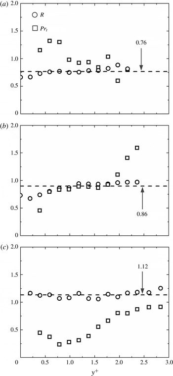
The distributions of
 $R$
and
 $Pr_{t}$
at all three
 $x^{+}$
positions are shown in figure 13. Because
 $y^{+}=0$
is a singular point of
 $Pr_{t}$
, the centreline values are not shown. Here,
 $Pr_{t}$
is of the order of one at
 $x^{+}=10$
, as reported by Antonia, Zhou & Matsumura (Reference Antonia, Zhou and Matsumura1993) and Zhou et al. (Reference Zhou, So, Liu and Zhang2000b
) for the same flow. Further downstream, the value of
 $Pr_{t}$
drops. By
 $x^{+}=40$
,
 $Pr_{t}$
shows more variation in the range of 0.20–0.75, which is consistent with Reynolds’ (Reference Reynolds1976) and Antonia et al.’s (Reference Antonia, Zhou and Matsumura1993) observations. The streamwise decrease in
 $Pr_{t}$
is mainly due to the fact that
 $\unicode[STIX]{x2202}\overline{\unicode[STIX]{x1D6E9}}/\unicode[STIX]{x2202}y$
diminishes more rapidly than
 $\unicode[STIX]{x2202}\overline{U}/\unicode[STIX]{x2202}y$
(Zhou et al.
Reference Zhou, So, Liu and Zhang2000b
), which is also evident in figure 4. This is also in agreement with Matsumura & Antonia’s (Reference Matsumura and Antonia1993) observation that Kármán vortices transport heat more effectively than momentum. It should be noted that
 $Pr_{t}$
is also
 $Re$
-dependent and increases with increasing
 $Re$
(Reynolds Reference Reynolds1976). That is why Berajeklian & Mydlarski (Reference Berajeklian and Mydlarski2011) observed a larger
 $Pr_{t}$
(ranging from 0.74 to 1.4) at
 $x^{+}=40$
of a cylinder wake, as their Re is as high as 24 300.
Relative to
 $Pr_{t}$
,
 $R$
does not vary appreciably across the wake, having an approximate mean value of 0.76, 0.86 and 1.12 at
 $x^{+}=10$
, 20 and 40 respectively. Béguier et al. (Reference Béguier, Dekeyser and Launder1978) reported a value of
 $R\approx 0.5$
in a self-preserving far wake, based on the isotropic mean scalar dissipation rate
 $\overline{\unicode[STIX]{x1D716}}_{\unicode[STIX]{x1D703}}=3\unicode[STIX]{x1D705}\overline{(\unicode[STIX]{x2202}\unicode[STIX]{x1D703}_{1}/\unicode[STIX]{x2202}x_{1})^{2}}$
and the isotropic mean turbulent kinetic energy dissipation rate
 $\overline{\unicode[STIX]{x1D716}}=15\unicode[STIX]{x1D708}\overline{(\unicode[STIX]{x2202}u_{1}/\unicode[STIX]{x2202}x_{1})^{2}}$
. The assumed isotropy may account for the difference in
 $R$
between the intermediate and far wakes. Under the effect of the large-scale coherent motions, the present flow is far from isotropic in the context of both
 $\overline{\unicode[STIX]{x1D700}}$
and
 $\overline{\unicode[STIX]{x1D712}}$
for both the enstrophy and the scalar dissipation rate. In particular, the scalar dissipation field is largely anisotropic even in the far wake. Antonia & Browne (Reference Antonia and Browne1986) demonstrated that the departure of the scalar dissipation rate from isotropy is in the range 50 %–100 % between the centreline and the free stream in the self-preserving far wake. Analytically, the time scale of a passive scalar fluctuation destroyed by the molecular motion in the fine scale is
 $$\begin{eqnarray}T_{\unicode[STIX]{x1D703}}=\frac{\unicode[STIX]{x1D702}_{B}^{2}}{\unicode[STIX]{x1D705}},\end{eqnarray}$$
and is equal to the time scale of the turbulent kinetic energy dissipated in the smallest scale,
 $$\begin{eqnarray}T_{q}=\frac{\unicode[STIX]{x1D702}^{2}}{\unicode[STIX]{x1D708}},\end{eqnarray}$$
since
 $$\begin{eqnarray}\frac{T_{\unicode[STIX]{x1D703}}}{T_{q}}=\frac{\unicode[STIX]{x1D702}_{B}^{2}\unicode[STIX]{x1D708}}{\unicode[STIX]{x1D702}^{2}\unicode[STIX]{x1D705}}=\frac{(\unicode[STIX]{x1D708}\unicode[STIX]{x1D705}^{2}/\overline{\unicode[STIX]{x1D716}})^{1/2}\unicode[STIX]{x1D708}}{(\unicode[STIX]{x1D708}^{3}/\overline{\unicode[STIX]{x1D716}})^{1/2}\unicode[STIX]{x1D705}}=1.\end{eqnarray}$$
This is fully consistent with the observation that
 $R$
approaches unity between
 $x^{+}=10$
and 20, and then slightly exceeds unity at
 $x^{+}=40$
, as the mixing between the shedded warm fluid and the entrained cold fluid is continuously improved, as is the homogeneity of the temperature field (e.g. figure 4 in Matsumura & Antonia (Reference Matsumura and Antonia1993)) between
 $x^{+}=10$
and
 $x^{+}=40$
. One may expect that
 $R$
will reach unity provided that heat is homogeneously mixed, as observed in homogeneous grid turbulence by Yeh & Atta (Reference Yeh and Atta1973), Warhaft & Lumley (Reference Warhaft and Lumley1978) and Zhou et al. (Reference Zhou, Antonia, Danaila and Anselmet2000a
).
8 Conclusions
The similarity between the enstrophy and the temperature dissipation rate, as well as that between the turbulent kinetic energy and the passive scalar variance, have been examined in the turbulent intermediate wake of a circular cylinder at a Reynolds number of
 $2.5\times 10^{3}$
, in both spectral and physical spaces. Three major conclusions can be drawn from this investigation.
(i) There is a reasonably close similarity between
 $F_{\unicode[STIX]{x1D712}}$
and
 $F_{\unicode[STIX]{x1D714}}$
, especially at
 $x^{+}=20$
and 40. Departures between the two spectra occur mainly at or near the wavenumber corresponding to the Kármán vortex frequency, namely
 $St=0.21$
. These departures, clearly caused by the Kármán vortices, diminish as
 $y/L$
increases from 0 to 2 or
 $x^{+}$
increases from 10 to 40. Although the isocontours of the phase-averaged enstrophy are distinctly different from those of the phase-averaged scalar dissipation rate (figure 8), the contribution from the coherent structures to
 $\overline{\unicode[STIX]{x1D714}_{i}^{+}\unicode[STIX]{x1D714}_{i}^{+}}$
and
 $\overline{\unicode[STIX]{x1D703}_{,i}^{+}\unicode[STIX]{x1D703}_{,i}^{+}}$
is small (table 3), especially at
 $x^{+}=20$
and 40. Consequently, the remainder or relatively small-scale motions dominate the dissipation process. The isocontours of
 $\langle \unicode[STIX]{x1D714}_{ri}^{+}\unicode[STIX]{x1D714}_{ri}^{+}\rangle$
resemble those of
 $\langle \unicode[STIX]{x1D703}_{r,i}^{+}\unicode[STIX]{x1D703}_{r,i}^{+}\rangle$
(figure 9). As such, the similarity between
 $F_{\unicode[STIX]{x1D714}}$
and
 $F_{\unicode[STIX]{x1D712}}$
is only marginally affected by the highly coherent motions, particularly at
 $x^{+}=40$
. Nonetheless, the similarity between
 $F_{\unicode[STIX]{x1D714}}$
and
 $F_{\unicode[STIX]{x1D712}}$
is improved at
 $y/L=1$
, where the mean shear is large, by comparison with the centreline or the outer region of the wake where
 $\unicode[STIX]{x2202}\overline{U}/\unicode[STIX]{x2202}y$
is essentially zero or negligibly small. One may expect that the similarity between
 $F_{\unicode[STIX]{x1D714}}$
and
 $F_{\unicode[STIX]{x1D712}}$
may be further enhanced as
 $x^{+}$
increases beyond 40 due to the complete eradication of the Kármán vortex street.
(ii) The similarity between
 $F_{q}$
and
 $F_{\unicode[STIX]{x1D703}}$
is not good, especially in comparison with that between
 $F_{\unicode[STIX]{x1D714}}$
and
 $F_{\unicode[STIX]{x1D712}}$
. Clearly, the former similarity relates to energy containing scales (
 $\overline{q^{2}}$
and
 $\overline{\unicode[STIX]{x1D703}^{2}}$
) of turbulence, whereas the latter pertains to the small scales (
 $\overline{\unicode[STIX]{x1D714}_{i}\unicode[STIX]{x1D714}_{i}}$
and
 $\overline{\unicode[STIX]{x1D703}_{,i}\,\unicode[STIX]{x1D703}_{,i}}$
), which are not significantly affected by the large-scale organization even at the relatively low
 $Re$
of this study. The terms
 $F_{\unicode[STIX]{x1D703}}$
and
 $F_{u}$
exhibit a much better similarity than
 $F_{\unicode[STIX]{x1D703}}$
and
 $F_{q}$
, irrespective of
 $x^{+}$
. This observation is largely ascribed to the presence of a highly coherent
 $v$
fluctuation, since
 $F_{v}$
makes a large contribution to
 $F_{q}$
at a wavenumber corresponding approximately to
 $St=0.21$
, where
 $F_{\unicode[STIX]{x1D703}}$
differs greatly from
 $F_{q}$
. This assertion is supported by the fact that in physical space the coherent contributions to
 $\overline{u^{2}}$
and
 $\overline{\unicode[STIX]{x1D703}^{2}}$
are comparable but substantially smaller than that to
 $\overline{q^{2}}$
. The similarity between
 $F_{\unicode[STIX]{x1D703}}$
and
 $F_{u}$
is excellent around
 $y/L=1$
but deteriorates either at the centreline or as the free stream is approached. This suggests that the large magnitudes of the mean velocity and temperature gradients at
 $y/L=1$
also act to provide forcing to promote the similarity between
 $F_{\unicode[STIX]{x1D703}}$
and
 $F_{u}$
, although this forcing remains inadequate to influence the similarity between
 $F_{\unicode[STIX]{x1D703}}$
and
 $F_{q}$
to a significant extent. The situation is quite different in the far wake, where the similarity between
 $F_{\unicode[STIX]{x1D703}}$
and
 $F_{q}$
is quite good in the region where
 $\unicode[STIX]{x2202}\overline{U}/\unicode[STIX]{x2202}y$
and
 $\unicode[STIX]{x2202}\overline{\unicode[STIX]{x1D6E9}}/\unicode[STIX]{x2202}y$
are important. These terms, through their interactions with
 $\overline{uv}$
and
 $\overline{v\unicode[STIX]{x1D703}}$
, are source or production terms for
 $\overline{q^{2}}$
and
 $\overline{\unicode[STIX]{x1D703}^{2}}$
(Fulachier & Antonia Reference Fulachier and Antonia1984). This extra contribution to
 $\overline{q^{2}}$
and
 $\overline{\unicode[STIX]{x1D703}^{2}}$
is effective since the large-scale organized structures in the far wake, identified by Antonia, Browne & Bisset (Reference Antonia, Browne, Bisset and Fulachier1987) and Bisset, Antonia & Browne (Reference Bisset, Antonia and Browne1990), provide only weak contributions to
 $\overline{q^{2}}$
and
 $\overline{\unicode[STIX]{x1D703}^{2}}$
.
(iii) The dissipation time scale ratio
 $R$
does not vary significantly across the wake, compared with the turbulent Prandtl number; this disparity is especially large at
 $x^{+}=40$
. The magnitude of
 $R$
increases gradually from 0.76 at
 $x^{+}=10$
to 1.12 at
 $x^{+}=40$
, approaching the analytical value, i.e. 1, for a scalar homogeneously mixed by the turbulent motion. The difference between the present distribution of
 $R$
and that reported by Béguier et al. (Reference Béguier, Dekeyser and Launder1978) in the far wake can possibly be ascribed to the anisotropy of the scalar dissipation rate in the far wake (Antonia & Browne Reference Antonia and Browne1986). This is consistent with Sreenivasan’s (Reference Sreenivasan1991) argument that local isotropy is not a natural concept for scalars in turbulent shear flows.
The present study indicates that the processes that underpin the dissipations of the turbulent kinetic energy and scalar variance are intrinsically linked. The major contributions to these dissipations reside approximately over the same scales despite the presence of the coherent motion. This is in accord with the first similarity hypotheses enunciated by Kolmogorov (Reference Kolmogorov1941) and Obukhov (Reference Obukhov1949) for the small-scale velocity and temperature fields respectively. The similarity observed here at small
 $Re$
is expected to further improve as
 $Re$
increases. When
 $Re$
becomes sufficiently large for an inertial range to hold, (1.1) and (1.2) will apply, and the similarity between the passive scalar and velocity fields will extend to scales up to the end of the inertial range. On the other hand, as observed, at the small
 $Re$
of our study, the similarity between the two fields will hold over the dissipative scales; that is, the first similarity hypotheses of Kolmogorov (Reference Kolmogorov1941) and Obukhov (Reference Obukhov1949) are validated; the second hypotheses, which will lead, inter alia, to (1.1) and (1.2), will only hold at much larger
 $Re$
.
Acknowledgements
Y.Z. wishes to acknowledge financial support from the Scientific Research Fund of Shenzhen Government through grant JCYJ20140417172417119 and from the National Science Foundation of China through grant 11632006. R.A.A. acknowledges the support of ARC.