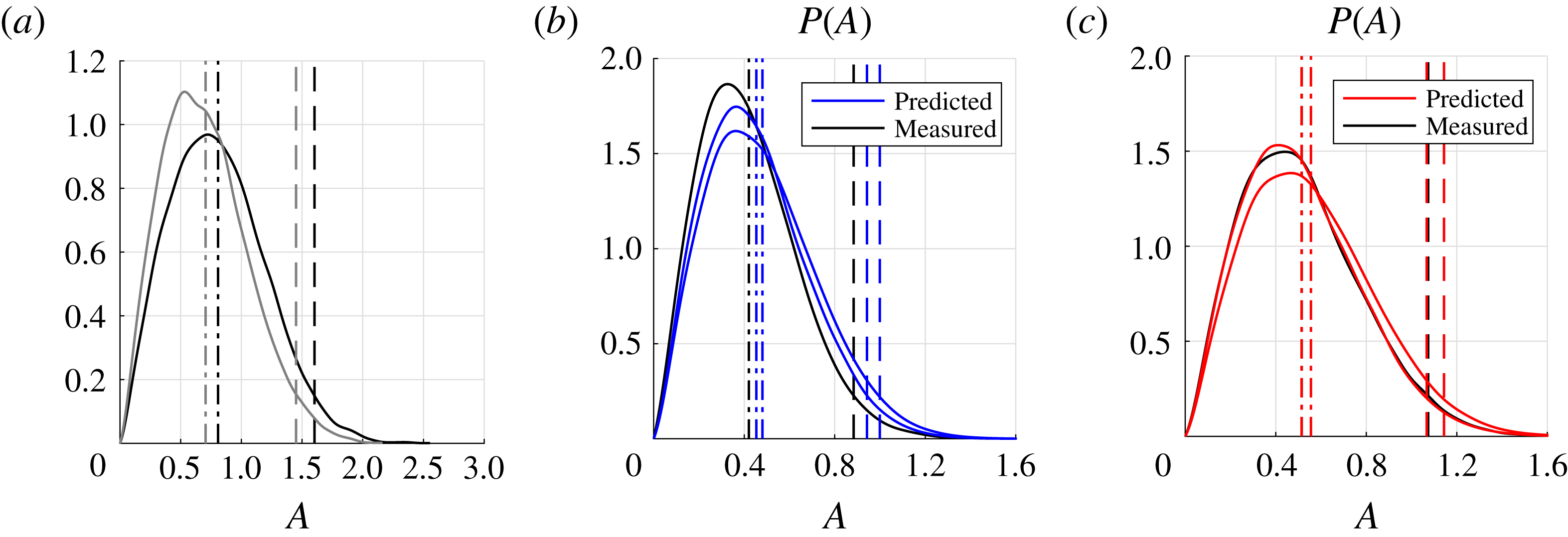
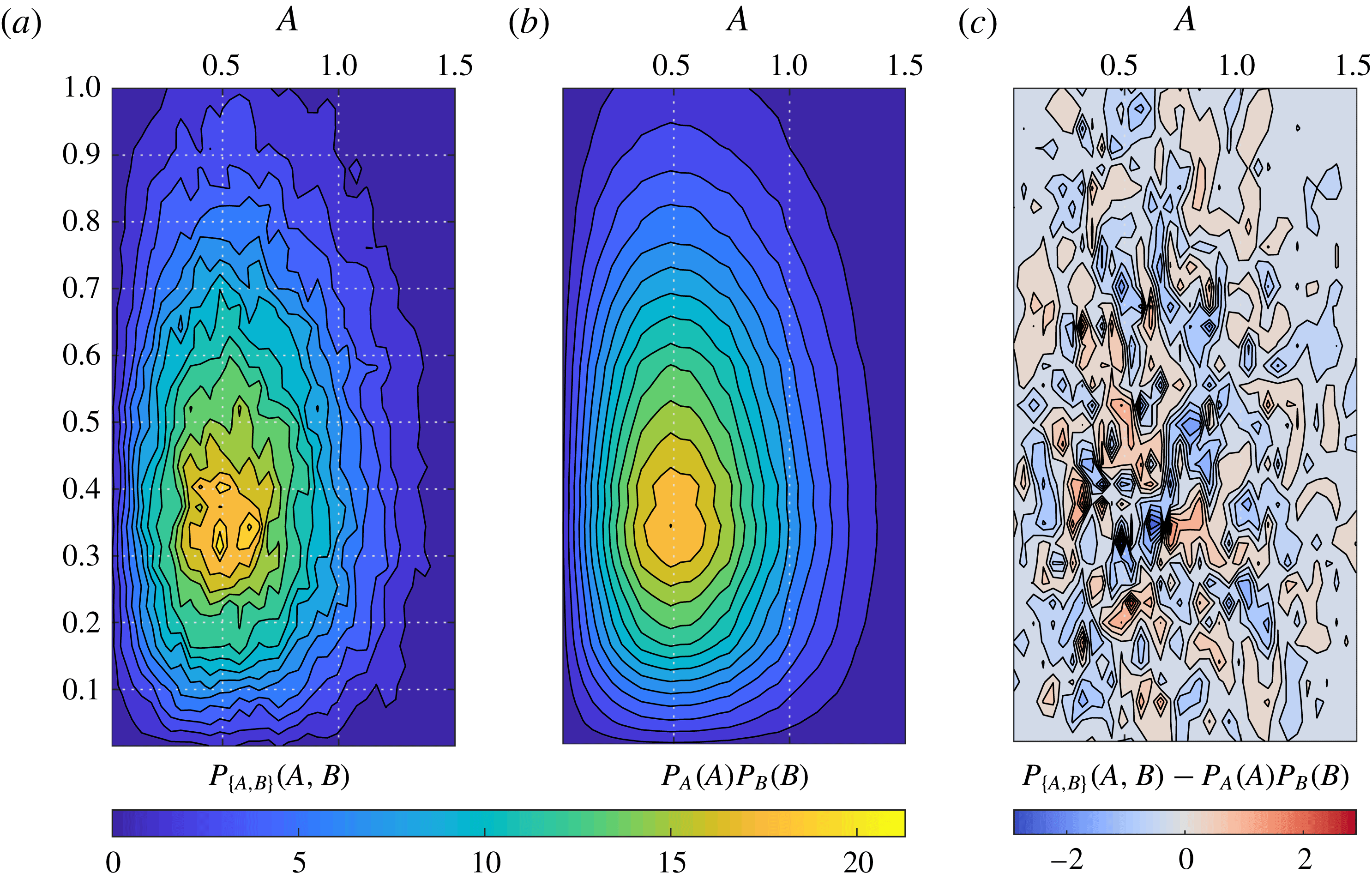
1 Introduction
A thermoacoustic instability can occur because of the feedback loop between an acoustic field and a fluctuating heat release rate response to it. It often converges to an attractor solution that exhibits a narrowband spectrum centred around a frequency
 $\unicode[STIX]{x1D714}$
plus its harmonics, as a result of the dynamic balance of acoustic energy between the flame response and the acoustic losses of the system.
One can model the flame response and the acoustic losses with linear transfer functions and predict the stability boundary of the linearized system with a stability analysis. This analysis can be extended to the nonlinear regime by making use of describing functions (Gelb & Vander Velde Reference Gelb and Vander Velde1968), which allow one to predict the amplitude and frequency of oscillations in the unstable regions (Dowling Reference Dowling1999; Noiray et al. Reference Noiray, Durox, Schuller and Candel2008; Boudy et al. Reference Boudy, Durox, Schuller, Jomaas and Candel2011b ). With this approach, the coherent response of the flame to a sinusoidal acoustic field is modelled as a function of the amplitude of pulsation, while the incoherent background combustion noise is discarded. A whole body of work (Culick et al. Reference Culick, Paparizos, Sterling and Burnley1992, Lieuwen Reference Lieuwen2003b , and references therein) has investigated how this background noise has an important role both in affecting the temporal dynamics of the system and in determining the amplitude of oscillation.
Wagner, Christoph & Sattelmayer (Reference Wagner, Christoph and Sattelmayer2013), Mejia, Miguel-Brebion & Selle (Reference Mejia, Miguel-Brebion and Selle2016) and Noiray (Reference Noiray2016) analysed the measured time series of a thermoacoustic system exhibiting a noisy attractor solution with a dominant frequency peak. They reviewed different techniques to estimate the linear growth rate that the system would manifest if the noisy term was artificially shut off from the equations. Other recent studies have compared the linear growth rates estimated from time series of an experiment with the numerical linear growth rate predictions of a low-order model; see, e.g., Bothien, Noiray & Schuermans (Reference Bothien, Noiray and Schuermans2015), Stadlmair et al. (Reference Stadlmair, Wagner, Hirsch and Sattelmayer2015), Hummel et al. (Reference Hummel, Berger, Schuermans and Sattelmayer2016). We show in this paper that it is possible and easier to predict the full nonlinear behaviour of the system instead of focusing on the linear behaviour that the system would manifest in the non-physical scenario of setting the background noise to zero. In particular, one can predict the probability density functions (PDFs) of the amplitudes of oscillation instead of characterizing linear growth rates. The predicted PDFs of the amplitude of acoustic pressure can be directly compared with the experimental PDFs. This new perspective shifts the focus from eigenvalue problems and respective growth rates in the linear and nonlinear regimes to stochastic differential equations and PDFs.
The theory is presented in § 2, the experimental validation in § 3 and the conclusions in § 4.
2 Theory
We introduce the governing equations and key assumptions on the problem in § 2.1 and the heat release rate model in § 2.2. In §§ 2.3 and 2.4, we briefly apply a well-known perturbation technique to the problem, to obtain in § 2.5 a single oscillator model, which is further simplified in § 2.6. In § 2.7, we apply stochastic averaging and obtain the expression for the PDF of the acoustic pressure amplitude in the combustor. In § 2.8, we discuss how one can use these results to identify the flame response from time series data, and in § 2.9, how to predict the new state of a thermoacoustic system when a change is applied to it, e.g. the installation of Helmholtz dampers.
2.1 Governing equations
We study the problem in terms of the pressure
 $p$
, the density
 $\unicode[STIX]{x1D70C}$
, the entropy
 $s$
and the three-dimensional velocity field
 $\boldsymbol{u}$
. We express each variable
 $f$
as the sum of a steady component
 $f_{0}$
and a fluctuating time-dependent acoustic component
 $f_{1}$
,

where
 $\boldsymbol{x}$
and
 $t$
are respectively a three-dimensional coordinate and the time variable.
In (2.1), we assume that the steady velocity field
 $\boldsymbol{u}_{0}$
is zero, i.e. make a zero-Mach-number
 $M$
assumption, which we discuss next. The Mach number affects the frequencies and mode shapes of the thermoacoustic modes and causes jumps in the acoustic pressure mode shapes at sudden changes of cross section area and across the flame. In particular, (1) the effect on the frequencies scales like
 $O(M^{2})$
(Dowling & Stow Reference Dowling and Stow2003), (2) the jump of the acoustic pressure at area changes is related to the steady pressure loss/recovery due to the change of cross section area and scales like
 $O(M)$
(Paschereit & Polifke Reference Paschereit and Polifke1998), (3) the jump of the acoustic pressure across the flame scales like
 $O(M)$
(Lieuwen Reference Lieuwen2001c
, equation (8)). In land-based gas turbine combustors, the Mach number is low and these effects are negligible. In particular, the jumps on the acoustic pressure mentioned earlier cannot be observed in the measured burner transfer matrices of industrial burners (Paschereit & Polifke Reference Paschereit and Polifke1998; Bellucci et al.
Reference Bellucci, Schuermans, Nowak, Flohr and Paschereit2005), validating the hypothesis of a zero-Mach-number assumption in (2.1).
Under the zero-Mach-number assumption, one can prove from the momentum equation that the steady acoustic pressure
 $p_{0}$
does not depend on space. We also assume that the unburnt and burnt gas mixtures are perfect gases, i.e. the equation of state
 $p=\unicode[STIX]{x1D70C}RT$
applies, where the specific gas constant
 $R$
of the gas mixture and the adiabatic ratio
 $\unicode[STIX]{x1D6FE}=C_{p}/C_{v}$
are independent of the temperature
 $T$
.
We linearize the equations of conservation of mass, momentum, energy, the transport equation of entropy and the gas state equation around the steady fields
 $\{p_{0},\unicode[STIX]{x1D70C}_{0},s_{0}\}$
, assuming that the fluctuations
 $\{p_{1},\unicode[STIX]{x1D70C}_{1},s_{1},\boldsymbol{u}_{1}\}$
are small. For example, the fluctuations of the pressure
 $p_{1}$
are of the order of 1 %–2 % of
 $p_{0}$
, as found by Scarinci (Reference Scarinci, Lieuwen and Yang2005, § II) in a land-based aeroderivative gas turbine. Neglecting viscous losses and heat diffusion, one obtains the equations governing the evolution of the acoustic pressure
 $p_{1}$
and the acoustic velocity
 $\boldsymbol{u}_{1}$
, as reviewed, e.g., by Clavin, Kim & Williams (Reference Clavin, Kim and Williams1994, § A),
 $$\begin{eqnarray}\displaystyle \frac{1}{c^{2}}\frac{\unicode[STIX]{x2202}p_{1}}{\unicode[STIX]{x2202}t} & = & \displaystyle -\unicode[STIX]{x1D70C}_{0}\unicode[STIX]{x1D735}\boldsymbol{\cdot }\boldsymbol{u}_{1}+\frac{\unicode[STIX]{x1D6FE}-1}{c^{2}}q_{1},\end{eqnarray}$$
 $$\begin{eqnarray}\displaystyle \unicode[STIX]{x1D70C}_{0}\frac{\unicode[STIX]{x2202}\boldsymbol{u}_{1}}{\unicode[STIX]{x2202}t} & = & \displaystyle -\unicode[STIX]{x1D735}p_{1}.\end{eqnarray}$$
 $q_{1}$
is the fluctuating heat release rate of the combustion process which is discussed in the next subsection. The fields
 $\unicode[STIX]{x1D70C}_{0}=p_{0}/RT_{0}$
and
 $c=\unicode[STIX]{x1D6FE}RT_{0}$
are functions of the temperature field
 $T_{0}(\boldsymbol{x})$
and depend on space. In particular, they vary considerably between the two regions of unburnt and burnt gases, upstream and downstream of the flame. However, the product
 $\unicode[STIX]{x1D70C}_{0}c^{2}=\unicode[STIX]{x1D6FE}p_{0}$
is constant, so we decide to multiply (2.2a
) by
 $c^{2}$
and obtain
 $$\begin{eqnarray}\displaystyle \frac{\unicode[STIX]{x2202}p_{1}}{\unicode[STIX]{x2202}t} & = & \displaystyle -\unicode[STIX]{x1D6FE}p_{0}\unicode[STIX]{x1D735}\boldsymbol{\cdot }\boldsymbol{u}_{1}+(\unicode[STIX]{x1D6FE}-1)q_{1},\end{eqnarray}$$
 $$\begin{eqnarray}\displaystyle \unicode[STIX]{x1D70C}_{0}\frac{\unicode[STIX]{x2202}\boldsymbol{u}_{1}}{\unicode[STIX]{x2202}t} & = & \displaystyle -\unicode[STIX]{x1D735}p_{1},\end{eqnarray}$$
 $\unicode[STIX]{x1D6FA}$
of the combustor, with boundary
 $\unicode[STIX]{x2202}\unicode[STIX]{x1D6FA}$
.
We now discuss the boundary conditions. On all walls of the combustor, we have that
 $\boldsymbol{u}_{1}\boldsymbol{\cdot }\boldsymbol{n}=0$
, where
 $\boldsymbol{n}$
is the unit vector orthogonal to the boundary
 $\unicode[STIX]{x2202}\unicode[STIX]{x1D6FA}$
, pointing outwards. At the compressor outlet and the turbine inlet, we impose an incoming acoustic velocity
 $u_{\bot }$
,
 $$\begin{eqnarray}\displaystyle \boldsymbol{u}_{1}\boldsymbol{\cdot }\boldsymbol{n}=-u_{\bot }\quad \text{at inlet and outlet}, & & \displaystyle\end{eqnarray}$$
where the sign convention on
 $u_{\bot }$
is such that
 $u_{\bot }(\boldsymbol{x},t)$
is positive when mass is added to the domain
 $\unicode[STIX]{x1D6FA}$
. We then relate the incoming velocity
 $u_{\bot }$
to the local value of the pressure through the reduced admittance
 ${\mathcal{Y}}$
,
 $$\begin{eqnarray}\displaystyle {\mathcal{Y}}\equiv \frac{u_{\bot }}{p/(\unicode[STIX]{x1D70C}_{0}c)}=\frac{{\mathcal{R}}-1}{{\mathcal{R}}+1}, & & \displaystyle\end{eqnarray}$$
where
 ${\mathcal{R}}$
is the reflection coefficient of an acoustic wave travelling in the outer direction being reflected inside the domain on the boundary
 $\unicode[STIX]{x2202}\unicode[STIX]{x1D6FA}$
. Because the flow is nearly choked at inlet and outlet (Lieuwen & Yang Reference Lieuwen and Yang2005), the boundary condition is largely reflective (Marble & Candel Reference Marble and Candel1977), i.e. the gain of the reflection coefficient
 ${\mathcal{R}}$
on the boundary is close to unity at the low frequencies of interest, as discussed for a realistic configuration by Bauerheim et al. (Reference Bauerheim, Duran, Livebardon, Wang, Moreau and Poinsot2016). Under these conditions of strong reflection on the upstream and downstream boundaries, Hoeijmakers et al. (Reference Hoeijmakers, Kornilov, Lopez Arteaga, de Goey and Nijmeijer2014), Emmert, Bomberg & Polifke (Reference Emmert, Bomberg and Polifke2015), Silva et al. (Reference Silva, Emmert, Jaensch and Polifke2015) and Poinsot (Reference Poinsot2016) find that the thermoacoustic modes are manifested as a perturbation of acoustic modes. We assume that the thermoacoustic modes are manifested as a perturbation of acoustic modes, rather being the recently identified intrinsic modes associated only with the flame response.
Combining (2.3), we obtain the inhomogeneous wave equation
 $$\begin{eqnarray}\displaystyle \frac{\unicode[STIX]{x2202}^{2}p_{1}}{\unicode[STIX]{x2202}t^{2}}-\unicode[STIX]{x1D6FE}p_{0}\unicode[STIX]{x1D735}\boldsymbol{\cdot }\left(\frac{\unicode[STIX]{x1D735}p_{1}}{\unicode[STIX]{x1D70C}_{0}}\right)=(\unicode[STIX]{x1D6FE}-1)\frac{\unicode[STIX]{x2202}q_{1}}{\unicode[STIX]{x2202}t}. & & \displaystyle\end{eqnarray}$$
2.2 Heat release rate model
We model the heat release rate
 $q_{1}$
coming from the flame as the sum of two contributions (Chiu & Summerfield Reference Chiu and Summerfield1974; Rajaram & Lieuwen Reference Rajaram and Lieuwen2009),
 $$\begin{eqnarray}\displaystyle q_{1}=q_{d}+q_{s}, & & \displaystyle\end{eqnarray}$$
where the subscripts
 $d$
and
 $s$
stand for deterministic and stochastic respectively. In (2.7), we distinguish between
 $q_{d}$
, which will be modelled as a function of the acoustic field at the excited thermoacoustic frequency, and
 $q_{s}$
, which represents the fluctuations of the heat release which are caused by physics that we neglect in the model. We discuss the two contributions in the following two subsections.
2.2.1 Deterministic part
The model for the deterministic heat release rate
 $q_{d}$
is the same as that presented in greater detail in Ghirardo, Juniper & Moeck (Reference Ghirardo, Juniper and Moeck2016), and is summarized here. The source term
 $q_{d}$
appearing on the right-hand side of (2.3a
) depends on the axial acoustic velocity at the burner (Fleifil et al.
Reference Fleifil, Annaswamy, Ghoneim and Ghoniem1996; Ducruix, Durox & Candel Reference Ducruix, Durox and Candel2000; Preetham & Lieuwen Reference Preetham and Lieuwen2008; Palies et al.
Reference Palies, Durox, Schuller and Candel2010) and/or at the fuel injection location (Lieuwen & Zinn Reference Lieuwen and Zinn1998; Bellucci et al.
Reference Bellucci, Schuermans, Paschereit and Flohr2001; Polifke, Kopitz & Serbanoviv Reference Polifke, Kopitz and Serbanoviv2001; Krebs et al.
Reference Krebs, Flohr, Prade and Hoffmann2002). For a review of both mechanisms, see Lieuwen (Reference Lieuwen2003a
), Schuermans et al. (Reference Schuermans, Bellucci, Güthe, Meili, Flohr and Paschereit2004) and Candel et al. (Reference Candel, Durox, Schuller, Bourgouin and Moeck2014).
One can express these acoustic velocities as the admittances of the whole part of the combustor upstream of their location multiplied by the local acoustic pressure, as long as only one axial mode or only a couple of azimuthal modes are excited. This is carried out in the modelling of one annular experimental rig by Ghirardo et al. (Reference Ghirardo, Juniper and Moeck2016, § 5.1), where the admittance of the whole part of the system upstream of the burner is modelled. We decide to lump the flame response
 $q_{1}$
as a nonlinear time-invariant operator
 ${\mathcal{Q}}$
of the acoustic pressure
 $p_{f}(t)$
at the flame location, noting that the acoustic pressure is the same both upstream and downstream of the flame,
 $$\begin{eqnarray}\displaystyle q_{d}(t)={\mathcal{Q}}[p_{f}(t)]. & & \displaystyle\end{eqnarray}$$
The operator
 ${\mathcal{Q}}$
is a nonlinear time-invariant operator and has memory of the past history of
 $p_{f}(t)$
. For example, Ghirardo et al. (Reference Ghirardo, Ćosić, Juniper and Moeck2015) choose a Hammerstein model for the operator
 ${\mathcal{Q}}$
. Equation (2.8) allows us later to consider a set of equations where everything depends on the pressure. The describing function
 $Q(A,\unicode[STIX]{x1D714})$
of the operator
 ${\mathcal{Q}}$
is defined as
 $$\begin{eqnarray}\displaystyle Q(A,\unicode[STIX]{x1D714})\equiv \frac{1}{A}\frac{1}{\unicode[STIX]{x03C0}/\unicode[STIX]{x1D714}}\int _{0}^{2\unicode[STIX]{x03C0}/\unicode[STIX]{x1D714}}{\mathcal{Q}}[A\cos (\unicode[STIX]{x1D714}t)]\text{e}^{-\text{i}\unicode[STIX]{x1D714}t}\,\text{d}t. & & \displaystyle\end{eqnarray}$$
The describing function
 $Q(A,\unicode[STIX]{x1D714})$
calculates the transfer function between one sinusoidal input
 $p(t)=A\cos (\unicode[STIX]{x1D714}t)$
and the respective output
 ${\mathcal{Q}}[p(t)]$
at a fixed level of the acoustic pressure amplitude
 $A$
. The dependence of
 $Q$
on the frequency
 $\unicode[STIX]{x1D714}$
is typical of transfer functions, while the dependence on the amplitude
 $A$
of acoustic pressure accounts for flames whose response depends nonlinearly on
 $A$
. This sets a describing function apart from a simpler transfer function, which can be used only for linear operators. In fact, if
 ${\mathcal{Q}}$
is linear, one can take
 $A$
out of the square brackets in (2.9) and simplify it, so that
 $Q$
would not depend on
 $A$
in the linear case. The real part of
 $Q$
describes the part of the heat release that is in phase with the input pressure, and in a combustor leads to a positive Rayleigh contribution if it is positive. Instead, the imaginary part of
 $Q$
is in quadrature with the input and is responsible for a shift of the thermoacoustic frequency. Both aspects will be covered in § 2.7.
We observe that the describing function
 $Q(A,\unicode[STIX]{x1D714})$
defined as in (2.9) does not fully describe the original operator
 ${\mathcal{Q}}[p]$
in two ways. First, it does not capture the additional response of
 ${\mathcal{Q}}$
at frequencies that are multiples of
 $\unicode[STIX]{x1D714}$
. Under the assumption that no system resonance is found at these frequencies, this additional response can be typically neglected in a broad class of systems exhibiting low-pass filter behaviour above
 $\unicode[STIX]{x1D714}$
(Gelb & Vander Velde Reference Gelb and Vander Velde1968), as often assumed in thermoacoustics. Second, the definition (2.9) describes the response to steady sinusoidal input with real valued
 $\unicode[STIX]{x1D714}$
, without capturing transients. For example, when the input amplitude
 $A$
grows from one value
 $A_{1}$
to a second value
 $A_{2}$
, the operator
 ${\mathcal{Q}}[p(t)]$
will show correctly a delayed response, where the internal state of
 ${\mathcal{Q}}$
keeps memory of
 $A_{1}$
for some time. However, the describing function
 $Q(A(t),\unicode[STIX]{x1D714})$
will show a sudden change as soon as
 $A$
changes from
 $A_{1}$
. This deficiency of the describing function is not noticeable when the system is at a steady amplitude, typical of stable limit cycles in deterministic systems. It has, however, an effect on the dynamics when stochastic noise is considered, because physically noise pushes the system away from the limit cycle and leads to transient system response. We will reconsider this assumption in the conclusions.
2.2.2 Stochastic part
In this subsection, we discuss the heat release rate fluctuations
 $q_{s}$
that occur regardless of the coherent acoustic field. These are sometimes referred to as background noise of the flame, are always present in turbulent flames and are the only observed fluctuations of flames studied in open flame configurations (Chiu & Summerfield Reference Chiu and Summerfield1974), where the classical acoustic feedback loop is not present (and we assume that no intrinsic instabilities occur, for simplicity). Strahle (Reference Strahle1971, Reference Strahle1972) discusses how this component typically has a spectrum with most of the energy in the low frequencies. Hedge, Reuter & Zinn (Reference Hedge, Reuter and Zinn1987) are probably the first to make use of the measured spectrum
 $q_{s}$
of the heat release rate of a stable flame to make predictions of the same flame in an unstable configuration. Rajaram & Lieuwen (Reference Rajaram and Lieuwen2009) review and discuss the spectra of open premixed flames, which emit only the component
 $q_{s}$
. They show that the non-dimensional spectra of
 $q_{s}$
collapse well for various cases and conditions. One then considers modelling of
 $q_{s}$
as a stochastic process that has no dependence on the state of the system. Culick et al. (Reference Culick, Paparizos, Sterling and Burnley1992) propose to model a generic additional stochastic source term as a white Gaussian noise
 $\tilde{\unicode[STIX]{x1D70E}}\unicode[STIX]{x1D709}(t)$
with autocovariance function
 $C_{\unicode[STIX]{x1D709}\unicode[STIX]{x1D709}}(\unicode[STIX]{x1D70F})=\tilde{\unicode[STIX]{x1D70E}}^{2}\unicode[STIX]{x1D6FF}(\unicode[STIX]{x1D70F})$
. This assumption is very convenient because of the analytical properties that white Gaussian noise has in the context of stochastic differential equations. It is also effective. In fact, recently, Bonciolini, Boujo & Noiray (Reference Bonciolini, Boujo and Noiray2017) studied the effect on a thermoacoustic problem of choosing two different additive sources of coloured noise, which in principle can mimic the same spectra of
 $q_{s}$
. They showed that these coloured noises lead to the same results of an equivalent additive white noise source. We then assume in the following that the noise is white, Gaussian and with unit variance, and will denote it with the symbol
 $\unicode[STIX]{x1D709}$
. Later in the paper,
 $q_{s}$
will appear in a spatial integral together with the eigenmode
 $\unicode[STIX]{x1D713}$
of interest,
 $$\begin{eqnarray}\displaystyle q_{s,pr}(t)\equiv \frac{\unicode[STIX]{x1D6FE}-1}{\unicode[STIX]{x1D6EC}}\int _{\unicode[STIX]{x1D6FA}}q_{s}(\boldsymbol{x},t)\unicode[STIX]{x1D713}(\boldsymbol{x})\,\text{d}V=\unicode[STIX]{x1D70E}\unicode[STIX]{x1D709}(t), & & \displaystyle\end{eqnarray}$$
where
 $\unicode[STIX]{x1D713}$
is a function of space and
 $\unicode[STIX]{x1D6EC}$
is a constant. We assume that the source term on the right-hand side of (2.10) is white Gaussian noise, with standard deviation
 $\unicode[STIX]{x1D70E}$
. We will discuss the effect of the stochastic part of the fluctuating heat release rate in § 2.7.
2.3 The conservative equations
In this section, we discuss the homogeneous problem, obtained by setting source terms to zero in the governing equations. By doing this, we recover a self-adjoint problem, for which a set of orthogonal eigenmodes exist. These modes, so-called Galerkin modes, allow a series expansion of the solution, which is employed later in § 2.4.
By setting
 $q_{1}=0$
in (2.6), we obtain the homogeneous wave equation
 $$\begin{eqnarray}\displaystyle {\mathcal{L}}[p]\equiv \frac{\unicode[STIX]{x2202}^{2}p}{\unicode[STIX]{x2202}t^{2}}-\unicode[STIX]{x1D6FE}p_{0}\unicode[STIX]{x1D735}\boldsymbol{\cdot }\left(\frac{\unicode[STIX]{x1D735}p}{\unicode[STIX]{x1D70C}_{0}}\right)=0. & & \displaystyle\end{eqnarray}$$
Despite having a first-order spatial derivative, the operator
 ${\mathcal{L}}$
is self-adjoint, as discussed by Morse & Feshback (Reference Morse and Feshback1953a
, chap. 8, p. 874). The problem is separable in the space and time coordinates, and one can look for a solution with structure
 $p(\boldsymbol{x},t)=\unicode[STIX]{x1D702}(t)\unicode[STIX]{x1D713}(\boldsymbol{x})$
,
 $$\begin{eqnarray}\displaystyle \ddot{\unicode[STIX]{x1D702}}(t)+\unicode[STIX]{x1D714}^{2}\unicode[STIX]{x1D702}(t) & = & \displaystyle 0,\end{eqnarray}$$
 $$\begin{eqnarray}\displaystyle \unicode[STIX]{x1D6FE}p_{0}\unicode[STIX]{x1D735}\boldsymbol{\cdot }\left(\frac{\unicode[STIX]{x1D735}\unicode[STIX]{x1D713}(\boldsymbol{x})}{\unicode[STIX]{x1D70C}_{0}}\right)+\unicode[STIX]{x1D714}^{2}\unicode[STIX]{x1D713}(\boldsymbol{x}) & = & \displaystyle 0,\end{eqnarray}$$
 $\unicode[STIX]{x1D714}$
such that (2.12b
) admits a solution. We choose the boundary condition
 $\unicode[STIX]{x1D735}\unicode[STIX]{x1D713}\boldsymbol{\cdot }\boldsymbol{n}=0$
on the boundary
 $\unicode[STIX]{x2202}\unicode[STIX]{x1D6FA}$
for the Helmholtz equation (2.12b
) because the flow is nearly choked at the inlet and outlet. We detail why this choice is appropriate in appendix A. Equation (2.12b
) is the eigenproblem
 $$\begin{eqnarray}\displaystyle {\mathcal{H}}[\unicode[STIX]{x1D713}]=\unicode[STIX]{x1D706}\unicode[STIX]{x1D713}, & & \displaystyle\end{eqnarray}$$
 $$\begin{eqnarray}\displaystyle \left.\begin{array}{@{}rcl@{}}{\mathcal{H}}[\unicode[STIX]{x1D713}]\,\, & \equiv \,\, & \unicode[STIX]{x1D6FE}p_{0}\unicode[STIX]{x1D735}\boldsymbol{\cdot }(\unicode[STIX]{x1D735}\unicode[STIX]{x1D713}/\unicode[STIX]{x1D70C}_{0}),\\ \unicode[STIX]{x1D706}\,\, & \equiv \,\, & -\unicode[STIX]{x1D714}^{2},\end{array}\right\} & & \displaystyle\end{eqnarray}$$
 $\unicode[STIX]{x1D706}$
. Because the domain is finite and boundary conditions are reflective, there is a countable set
 $\{(\unicode[STIX]{x1D714}_{n},\unicode[STIX]{x1D713}_{n}),n=1,2,\ldots \}$
of solutions of (2.13).
Since the problem is self-adjoint, the spectral theorem guarantees that the eigenfrequencies
 $\unicode[STIX]{x1D714}_{n}$
are real valued, that we can choose the eigenmodes
 $\unicode[STIX]{x1D713}_{n}$
to be real valued and that the set of eigenmodes are orthogonal,
 $$\begin{eqnarray}\displaystyle & \displaystyle \left.\begin{array}{@{}c@{}}\displaystyle \unicode[STIX]{x1D713}_{m}=\unicode[STIX]{x1D713}_{m}^{\ast },\\ \displaystyle \unicode[STIX]{x1D714}_{m}=\unicode[STIX]{x1D714}_{m}^{\ast },\end{array}\right\}\quad m=1,2,\ldots , & \displaystyle\end{eqnarray}$$
 $$\begin{eqnarray}\displaystyle & \displaystyle \int _{\unicode[STIX]{x1D6FA}}\unicode[STIX]{x1D713}_{m}(\boldsymbol{x})\unicode[STIX]{x1D713}_{n}^{\ast }(\boldsymbol{x})\,\text{d}V=\unicode[STIX]{x1D6EC}_{m}\unicode[STIX]{x1D6FF}_{mn},\quad m,n=1,2,\ldots , & \displaystyle\end{eqnarray}$$
 $$\begin{eqnarray}\displaystyle \int _{0}^{t}p_{1}(\boldsymbol{x},t^{\prime })\,\text{d}t^{\prime }=\mathop{\sum }_{m=1}^{\infty }\unicode[STIX]{x1D702}_{m}(t)\unicode[STIX]{x1D713}_{m}(\boldsymbol{x}), & & \displaystyle\end{eqnarray}$$
where
 $\unicode[STIX]{x1D702}_{m}(t)$
are the time-dependent coefficients, and we express with
 $t^{\prime }$
the time variable inside the integral. We then obtain the series expansions for the acoustic pressure and acoustic velocity fields,
 $$\begin{eqnarray}\displaystyle p_{1}(\boldsymbol{x},t) & = & \displaystyle \mathop{\sum }_{m=0}^{\infty }\dot{\unicode[STIX]{x1D702}}_{n}(t)\unicode[STIX]{x1D713}_{m}(\boldsymbol{x}),\end{eqnarray}$$
 $$\begin{eqnarray}\displaystyle \boldsymbol{u}_{1}(\boldsymbol{x},t) & = & \displaystyle -\mathop{\sum }_{m=0}^{\infty }\unicode[STIX]{x1D702}_{m}(t)\frac{\unicode[STIX]{x1D735}\unicode[STIX]{x1D713}_{m}(\boldsymbol{x})}{\unicode[STIX]{x1D70C}_{0}},\end{eqnarray}$$
where (2.15b
) is obtained by deriving (2.15a
) with respect to the time
 $t$
and (2.15c
) is obtained by substituting (2.15b
) in (2.3b
) and integrating by
 $t$
.
In this subsection, we have obtained a series expansion of the acoustic pressure
 $p_{1}$
and acoustic velocity
 $\boldsymbol{u}_{1}$
in (2.15) which is used in the following as ansatz for the original equation (2.6). The mode
 $\unicode[STIX]{x1D713}_{m}(\boldsymbol{x})$
is the
 $m$
th Galerkin mode, and
 $\unicode[STIX]{x1D702}_{m}(t)$
is the corresponding time-dependent amplitude.
2.4 Galerkin projection
In this subsection, we project the governing equations (2.6) on the Galerkin modes introduced in the previous subsection. This allows us to map the dynamics from a partial differential equation to a set of ordinary differential equations.
We multiply (2.12b
) calculated for the
 $n$
th eigenmode by
 $\int _{0}^{t}p_{1}(\boldsymbol{x},t^{\prime })\,\text{d}t^{\prime }$
, and sum it to (2.3a
) multiplied by
 $\unicode[STIX]{x1D713}_{n}$
,
 $$\begin{eqnarray}\displaystyle & \displaystyle \unicode[STIX]{x1D6FE}p_{0}\unicode[STIX]{x1D735}\boldsymbol{\cdot }\left(\frac{\unicode[STIX]{x1D735}\unicode[STIX]{x1D713}_{n}}{\unicode[STIX]{x1D70C}_{0}}\right)\int _{0}^{t}p_{1}\,\text{d}t^{\prime }+\unicode[STIX]{x1D714}^{2}\unicode[STIX]{x1D713}_{n}\int _{0}^{t}p_{1}\,\text{d}t^{\prime }+\frac{\unicode[STIX]{x2202}p_{1}}{\unicode[STIX]{x2202}t}\unicode[STIX]{x1D713}_{n} & \displaystyle \nonumber\\ \displaystyle & \displaystyle +\,\unicode[STIX]{x1D6FE}p_{0}\unicode[STIX]{x1D735}\boldsymbol{\cdot }\boldsymbol{u}_{1}\unicode[STIX]{x1D713}_{n}=(\unicode[STIX]{x1D6FE}-1)q_{1}\unicode[STIX]{x1D713}_{n}. & \displaystyle\end{eqnarray}$$
We reorder the terms in the equation,
 $$\begin{eqnarray}\displaystyle & \displaystyle \frac{\unicode[STIX]{x2202}p_{1}}{\unicode[STIX]{x2202}t}\unicode[STIX]{x1D713}_{n}+\unicode[STIX]{x1D714}^{2}\unicode[STIX]{x1D713}_{n}\int _{0}^{t}p_{1}\,\text{d}t^{\prime }=(\unicode[STIX]{x1D6FE}-1)q_{1}\unicode[STIX]{x1D713}_{n}-\unicode[STIX]{x1D6FE}p_{0} & \displaystyle \nonumber\\ \displaystyle & \displaystyle \times ~\underbrace{\left[\unicode[STIX]{x1D735}\boldsymbol{\cdot }\left(\frac{\unicode[STIX]{x1D735}\unicode[STIX]{x1D713}_{n}}{\unicode[STIX]{x1D70C}_{0}}\right)\int _{0}^{t}p_{1}\,\text{d}t^{\prime }+\unicode[STIX]{x1D735}\boldsymbol{\cdot }\boldsymbol{u}_{1}\unicode[STIX]{x1D713}_{n}\right]}_{T}. & \displaystyle\end{eqnarray}$$
We integrate (2.17) over the whole domain
 $\unicode[STIX]{x1D6FA}$
,
 $$\begin{eqnarray}\displaystyle \int _{\unicode[STIX]{x1D6FA}}\frac{\unicode[STIX]{x2202}p_{1}}{\unicode[STIX]{x2202}t}\unicode[STIX]{x1D713}_{n}\,\text{d}V+\int _{\unicode[STIX]{x1D6FA}}\unicode[STIX]{x1D714}^{2}\unicode[STIX]{x1D713}_{n}\int _{0}^{t}p_{1}\,\text{d}t^{\prime }\,\text{d}V=\int _{\unicode[STIX]{x1D6FA}}(\unicode[STIX]{x1D6FE}-1)q_{1}\unicode[STIX]{x1D713}_{n}\,\text{d}V-\unicode[STIX]{x1D6FE}p_{0}\int _{\unicode[STIX]{x1D6FA}}T\,\text{d}V. & & \displaystyle\end{eqnarray}$$
We rewrite the last integral on the right-hand side of (2.18) as
 $$\begin{eqnarray}\displaystyle \int _{\unicode[STIX]{x1D6FA}}T\,\text{d}V & = & \displaystyle \int _{\unicode[STIX]{x1D6FA}}\unicode[STIX]{x1D735}\boldsymbol{\cdot }\left(\frac{\unicode[STIX]{x1D735}\unicode[STIX]{x1D713}_{n}}{\unicode[STIX]{x1D70C}_{0}}\right)\int _{0}^{t}p_{1}\,\text{d}t^{\prime }+\unicode[STIX]{x1D735}\boldsymbol{\cdot }\boldsymbol{u}_{1}\unicode[STIX]{x1D713}_{n}\,\text{d}V\nonumber\\ \displaystyle & = & \displaystyle \int _{\unicode[STIX]{x1D6FA}}\unicode[STIX]{x1D735}\boldsymbol{\cdot }\left(\frac{\unicode[STIX]{x1D735}\unicode[STIX]{x1D713}_{n}}{\unicode[STIX]{x1D70C}_{0}}\int _{0}^{t}p_{1}\,\text{d}t^{\prime }+\boldsymbol{u}_{1}\unicode[STIX]{x1D713}_{n}\right)\text{d}V\nonumber\\ \displaystyle & & \displaystyle -\,\int _{\unicode[STIX]{x1D6FA}}\frac{\unicode[STIX]{x1D735}\unicode[STIX]{x1D713}_{n}}{\unicode[STIX]{x1D70C}_{0}}\boldsymbol{\cdot }\unicode[STIX]{x1D735}\left(\int _{0}^{t}p_{1}\,\text{d}t^{\prime }\right)+\boldsymbol{u}_{1}\boldsymbol{\cdot }\unicode[STIX]{x1D735}\unicode[STIX]{x1D713}_{n}\,\text{d}V.\end{eqnarray}$$
The second volume integral in (2.19) is zero because we substitute
 $\unicode[STIX]{x1D735}(\int _{0}^{t}p_{1}\,\text{d}t^{\prime })=-\unicode[STIX]{x1D70C}_{0}\boldsymbol{u}_{1}$
from (2.3b
) and the two terms in the argument of the integral cancel out. We apply the Green theorem to the first integral of (2.19),
 $$\begin{eqnarray}\displaystyle \int _{\unicode[STIX]{x1D6FA}}T\,\text{d}V=\int _{\unicode[STIX]{x2202}\unicode[STIX]{x1D6FA}}\left[\frac{1}{\unicode[STIX]{x1D70C}_{0}}\unicode[STIX]{x1D735}\unicode[STIX]{x1D713}_{n}\boldsymbol{\cdot }\boldsymbol{n}\int _{0}^{t}p_{1}\,\text{d}t^{\prime }+\boldsymbol{u}_{1}\boldsymbol{\cdot }\boldsymbol{n}\,\unicode[STIX]{x1D713}_{n}\right]\text{d}S. & & \displaystyle\end{eqnarray}$$
The integral of the first term in (2.20) is zero because we impose by construction
 $\unicode[STIX]{x1D735}\unicode[STIX]{x1D713}_{n}\boldsymbol{\cdot }\boldsymbol{n}=0$
on the boundary
 $\unicode[STIX]{x2202}\unicode[STIX]{x1D6FA}$
just before (2.12). We are left with
 $$\begin{eqnarray}\displaystyle \int _{\unicode[STIX]{x1D6FA}}T\,\text{d}V=\int _{\unicode[STIX]{x2202}\unicode[STIX]{x1D6FA}}\boldsymbol{u}_{1}\boldsymbol{\cdot }\boldsymbol{n}\,\unicode[STIX]{x1D713}_{n}\,\text{d}S=-\int _{\substack{ inlet \\ outlet}}u_{\bot }\unicode[STIX]{x1D713}_{n}\,\text{d}S. & & \displaystyle\end{eqnarray}$$
We substitute (2.15) and (2.21) in (2.18), exploit (2.14) and divide by
 $\unicode[STIX]{x1D6EC}_{n}$
,
 $$\begin{eqnarray}\displaystyle \ddot{\unicode[STIX]{x1D702}}_{n}+\unicode[STIX]{x1D714}_{n}^{2}\unicode[STIX]{x1D702}_{n}=\frac{\unicode[STIX]{x1D6FE}-1}{\unicode[STIX]{x1D6EC}_{n}}\int _{\unicode[STIX]{x1D6FA}}q_{1}\unicode[STIX]{x1D713}_{n}\,\text{d}V+\frac{\unicode[STIX]{x1D6FE}p_{0}}{\unicode[STIX]{x1D6EC}_{n}}\int _{\substack{ inlet \\ outlet}}u_{\bot }\unicode[STIX]{x1D713}_{n}\,\text{d}S\quad n=0,1,\ldots . & & \displaystyle\end{eqnarray}$$
We find in (2.22) that the amplitudes
 $\unicode[STIX]{x1D702}_{n}(t)$
of the eigenmodes
 $\unicode[STIX]{x1D713}_{n}(\boldsymbol{x})$
of the solution (2.15) are a set of oscillators. Each
 $n$
th oscillator is forced by two source terms, projected on the mode
 $\unicode[STIX]{x1D713}_{n}$
. The problem (2.22) is nonlinear because the operator
 ${\mathcal{Q}}$
appearing in the expressions (2.7) and (2.8) for the heat release rate response
 $q_{1}$
is nonlinear, and the oscillators
 $\unicode[STIX]{x1D702}_{n}$
interact with each other only via
 $q_{1}$
and the boundary conditions.
Similar equations are obtained by Morse & Feshback (Reference Morse and Feshback1953a
, p. 849) in terms of the Green function, and similarly reviewed by Culick (Reference Culick2006, chap. 4.3). There are, however, two differences from these references. First, we account for a spatial dependence of
 $c$
,
 $\unicode[STIX]{x1D70C}_{0}$
and
 $T_{0}$
, which makes the set of eigenmodes
 $\{\unicode[STIX]{x1D713}_{m},\unicode[STIX]{x1D714}_{m}\}$
very close to the thermoacoustic modes, except for the volume source
 $q_{1}\neq 0$
in (2.3) and the boundary source
 $u_{\bot }$
, which will be treated as a perturbation in the next subsection. In particular, the Galerkin modes account for the sudden jump in the acoustic velocity at the flame interface due to the temperature jump. Second, we choose in (2.15b
) the structure of the pressure as
 $\sum (\unicode[STIX]{x2202}\unicode[STIX]{x1D702}_{m}(t)/\unicode[STIX]{x2202}t)\unicode[STIX]{x1D713}_{m}$
instead of a structure like
 $\sum \unicode[STIX]{x1D712}_{m}(t)\unicode[STIX]{x1D713}_{m}$
, where
 $\unicode[STIX]{x1D712}_{m}$
is without time derivative. We then carry out the projection on the fluctuating pressure equation (2.3a
) instead of the usual wave equation. This leads to the set of dynamic equations (2.22), where the source term
 $q_{1}$
is present, instead of its time derivative
 $\unicode[STIX]{x2202}q_{1}/\unicode[STIX]{x2202}t$
, as presented, e.g., in Dowling & Stow (Reference Dowling and Stow2003, equation (36)) or in Schuermans, Paschereit & Monkewitz (Reference Schuermans, Paschereit and Monkewitz2006, equation (16)). This simplifies the physical interpretation of the equations later in § 2.7.
To achieve convergence of the series expansion (2.15b
) to the solution, one must formally consider all of the infinite modes
 $\unicode[STIX]{x1D702}_{n}(t),n=1,2,\ldots ,\infty$
in (2.22). However, each
 $n$
th oscillator responds little at frequencies far from its natural frequency
 $\unicode[STIX]{x1D714}_{n}$
, and self-excited thermoacoustic oscillations often have a very narrowband spectrum. Then, in certain applications, when the behaviour of a system is predicted over a certain frequency range, one truncates the set of equations to all of the modes with frequencies
 $\unicode[STIX]{x1D714}_{n}$
within that range. For example, Zinn & Lores (Reference Zinn and Lores1971) found that 10 eigenmodes were sufficient for time domain accuracy of a nonlinear simulation of an axial combustion instability in a rocket. The next section focuses instead on another application, when a self-excited thermoacoustic response is identified (as opposed to predicted), where a single mode is often sufficient.
2.5 The single oscillator model
In this subsection, we reduce the set of ordinary differential equations (2.22) obtained in the previous section to a single oscillator model because it is easier to manipulate analytically for the thermoacoustic system. This will be analysed later in § 2.7.
We substitute in (2.22) the heat release rate model from (2.7) and (2.8) and the boundary admittance
 $A$
introduced in (2.5),
 $$\begin{eqnarray}\displaystyle \ddot{\unicode[STIX]{x1D702}}_{n}+\unicode[STIX]{x1D714}_{n}^{2}\unicode[STIX]{x1D702}_{n} & = & \displaystyle \frac{\unicode[STIX]{x1D6FE}-1}{\unicode[STIX]{x1D6EC}_{n}}\int _{\unicode[STIX]{x1D6FA}}{\mathcal{Q}}\left[\mathop{\sum }_{m=0}^{\infty }\dot{\unicode[STIX]{x1D702}}_{m}\unicode[STIX]{x1D713}_{m}(\boldsymbol{x}_{f})\right]\unicode[STIX]{x1D713}_{n}\,\text{d}V+\frac{\unicode[STIX]{x1D6FE}-1}{\unicode[STIX]{x1D6EC}_{n}}\int _{\unicode[STIX]{x1D6FA}}q_{s}\unicode[STIX]{x1D713}_{n}\,\text{d}V\nonumber\\ \displaystyle & & \displaystyle +\,\frac{c}{\unicode[STIX]{x1D6EC}_{n}}\int _{\substack{ inlet \\ outlet}}{\mathcal{Y}}\left[\mathop{\sum }_{m=0}^{\infty }\dot{\unicode[STIX]{x1D702}}_{m}\unicode[STIX]{x1D713}_{m}\right]\unicode[STIX]{x1D713}_{n}\,\text{d}S\quad n=0,1,\ldots .\end{eqnarray}$$
The right-hand side of (2.23) is a regular perturbation of the homogeneous problem discussed in § 2.3, which modulates the amplitude of each oscillator. Morse & Feshback (Reference Morse and Feshback1953b
, chap. 9.1) present three iterative algorithms in the frequency domain that allow one to track how each eigenmode
 $\unicode[STIX]{x1D713}_{n}$
is perturbed, by fixing at the first iteration
 $\hat{p}^{(0)}(\boldsymbol{x},\unicode[STIX]{x1D714})=\unicode[STIX]{x1D713}_{n}(\boldsymbol{x})$
in the perturbation term, and calculate the resulting
 $\hat{p}^{(1)}$
iteratively from an integral formulation of the problem. In the frequency domain, each Galerkin mode is perturbed to a non-zero growth rate
 $\unicode[STIX]{x1D70E}$
and to a new frequency
 $\overline{\unicode[STIX]{x1D714}}_{n}$
shifted from the
 $\unicode[STIX]{x1D714}_{n}$
. The smallness of the perturbation term, which is the whole right-hand side of (2.23), can be discussed indirectly in terms of the non-dimensional growth rate
 $\unicode[STIX]{x1D70E}/\unicode[STIX]{x1D714}$
and the frequency shift
 $|\overline{\unicode[STIX]{x1D714}}_{n}-\unicode[STIX]{x1D714}_{n}|$
. A literature review of typical growth rates and frequency shifts caused by the flame is discussed in Ghirardo, Juniper & Bothien (Reference Ghirardo, Juniper and Bothien2017).
Culick (Reference Culick1988, § 4.3, and citations therein) reviews this method in detail for thermoacoustic applications. In particular, after his equation (4.10), he discusses how one can truncate the iterative procedure at the first step, i.e. approximate
 $p$
with just one Galerkin mode, and carry out only the first step of the derivation. In the time domain equation (2.23), this corresponds to ignoring all Galerkin modes except the one we want to identify. This approximation is often reasonable in thermoacoustic applications at low Mach numbers because the perturbation term is usually small. However, the shape of the Galerkin mode does not capture the sudden physical jump in acoustic velocity across the flame interface due to the flame response that is instead present in the exact thermoacoustic mode. Since in the following we will consider only this one mode, for convenience, we denote its eigenvector and amplitude as
 $\unicode[STIX]{x1D713}$
and
 $\unicode[STIX]{x1D702}$
respectively, so that
 $p(\boldsymbol{x},t)\approx \dot{\unicode[STIX]{x1D702}}(t)\unicode[STIX]{x1D713}(\boldsymbol{x})$
, and its eigenfrequency as
 $\unicode[STIX]{x1D714}_{0}$
. We also scale the mode
 $\unicode[STIX]{x1D713}$
so that
 $\unicode[STIX]{x1D713}(\boldsymbol{x}_{f})=1$
, and
 $\dot{\unicode[STIX]{x1D702}}(t)$
is then the acoustic pressure at the flame location
 $\boldsymbol{x}_{f}$
. By keeping only this mode in (2.23), and after substituting (2.10), we obtain
 $$\begin{eqnarray}\displaystyle & \displaystyle \ddot{\unicode[STIX]{x1D702}}+\unicode[STIX]{x1D714}_{0}^{2}\unicode[STIX]{x1D702}=\frac{\unicode[STIX]{x1D6FE}-1}{\unicode[STIX]{x1D6EC}}\int _{\unicode[STIX]{x1D6FA}}{\mathcal{Q}}[\dot{\unicode[STIX]{x1D702}}\unicode[STIX]{x1D713}(\boldsymbol{x}_{f})]\unicode[STIX]{x1D713}\,\text{d}V+\frac{\unicode[STIX]{x1D6FE}-1}{\unicode[STIX]{x1D6EC}_{n}}\int _{\unicode[STIX]{x1D6FA}}q_{s}\unicode[STIX]{x1D713}_{n}\,\text{d}V & \displaystyle \nonumber\\ \displaystyle & \displaystyle +\,\frac{c}{\unicode[STIX]{x1D6EC}_{n}}\int _{\substack{ inlet \\ outlet}}{\mathcal{Y}}[\dot{\unicode[STIX]{x1D702}}\unicode[STIX]{x1D713}]\unicode[STIX]{x1D713}\,\text{d}S. & \displaystyle\end{eqnarray}$$
Equation (2.24) is the fundamental equation that is discussed in § 2.7 and used in the experimental validation in § 3. The next subsection opens a parenthesis where (2.24) is simplified for some common applications.
2.6 Additional simplifications
In this subsection, we further simplify the source terms in (2.24), exploiting some features of the specific validation case discussed later in § 3. It should be noticed that these features add insight to the specific case at hand, but are not necessary for the following to hold. We assume a single acoustically compact flame, so that the first integral in (2.24) simplifies to
 $$\begin{eqnarray}\displaystyle \frac{\unicode[STIX]{x1D6FE}-1}{\unicode[STIX]{x1D6EC}}\int _{\unicode[STIX]{x1D6FA}}{\mathcal{Q}}[\dot{\unicode[STIX]{x1D702}}\unicode[STIX]{x1D713}]\unicode[STIX]{x1D713}\,\text{d}V=\frac{\unicode[STIX]{x1D6FE}-1}{\unicode[STIX]{x1D6EC}}{\mathcal{Q}}[\dot{\unicode[STIX]{x1D702}}\unicode[STIX]{x1D713}(\boldsymbol{x}_{f})]\unicode[STIX]{x1D713}(\boldsymbol{x}_{f}), & & \displaystyle\end{eqnarray}$$
where
 $\boldsymbol{x}_{f}$
is the flame position. We observe that the hypothesis of acoustic compactness regards only the direction of the acoustic pressure gradient. For example, for a purely azimuthal mode
 $\unicode[STIX]{x1D713}$
, which is constant in the axial direction, the acoustic compactness is required only in the direction where the mode varies, i.e. the azimuthal direction. Since we fixed
 $\unicode[STIX]{x1D713}(\boldsymbol{x}_{f})=1$
, (2.25) simplifies to
 $$\begin{eqnarray}\displaystyle \frac{\unicode[STIX]{x1D6FE}-1}{\unicode[STIX]{x1D6EC}}\int _{\unicode[STIX]{x1D6FA}}{\mathcal{Q}}[\dot{\unicode[STIX]{x1D702}}\unicode[STIX]{x1D713}]\unicode[STIX]{x1D713}\,\text{d}V=\frac{\unicode[STIX]{x1D6FE}-1}{\unicode[STIX]{x1D6EC}}{\mathcal{Q}}[\dot{\unicode[STIX]{x1D702}}]={\mathcal{Q}}_{pr}[\dot{\unicode[STIX]{x1D702}}], & & \displaystyle\end{eqnarray}$$
where we have introduced
 ${\mathcal{Q}}_{pr}$
for brevity. Of the second integral in (2.24), we consider only the outlet boundary, with the inlet boundary following similarly. Assuming that the admittance
 ${\mathcal{Y}}$
does not depend on the amplitude, the operator is linear and we can take the argument out of the square brackets. By also substituting (2.5) for
 ${\mathcal{Y}}$
, we obtain
 $$\begin{eqnarray}\displaystyle \frac{c}{\unicode[STIX]{x1D6EC}_{n}}\int _{outlet}{\mathcal{Y}}[\dot{\unicode[STIX]{x1D702}}\unicode[STIX]{x1D713}]\unicode[STIX]{x1D713}\,\text{d}S=-\left[\frac{c}{\unicode[STIX]{x1D6EC}_{n}}\frac{1-R}{1+R}\int _{outlet}\unicode[STIX]{x1D713}^{2}\,\text{d}S\right]\dot{\unicode[STIX]{x1D702}}. & & \displaystyle\end{eqnarray}$$
Because the flow is nearly choked at both compressor outlet and turbine inlet, the value of the gain of
 $R$
is close to unity (Marble & Candel Reference Marble and Candel1977). We also assume that
 $R$
is real valued by making a zero-Helmholtz-number approximation, since the first vane at the turbine inlet is axially acoustically compact compared with the acoustic wavelength of interest. It follows that the term between square brackets in (2.27) does not depend on frequency and is an equivalent damping coefficient
 $\unicode[STIX]{x1D6FC}>0$
,
 $$\begin{eqnarray}\displaystyle \frac{c}{\unicode[STIX]{x1D6EC}_{n}}\int _{\substack{ inlet \\ outlet}}{\mathcal{Y}}[\dot{\unicode[STIX]{x1D702}}\unicode[STIX]{x1D713}]\unicode[STIX]{x1D713}\,\text{d}S=-\unicode[STIX]{x1D6FC}\dot{\unicode[STIX]{x1D702}}. & & \displaystyle\end{eqnarray}$$
By substituting (2.26), (2.28) and (2.10) in (2.24), we obtain
 $$\begin{eqnarray}\displaystyle \ddot{\unicode[STIX]{x1D702}}+\unicode[STIX]{x1D714}_{0}^{2}\unicode[STIX]{x1D702}={\mathcal{Q}}_{pr}[\dot{\unicode[STIX]{x1D702}}]-\unicode[STIX]{x1D6FC}\dot{\unicode[STIX]{x1D702}}+\unicode[STIX]{x1D70E}\unicode[STIX]{x1D709}(t). & & \displaystyle\end{eqnarray}$$
One can account for a finite Helmholtz number at the turbine inlet by artificially extending the domain in the axial direction to account for a first-order Helmholtz number correction, as proposed by Stow, Dowling & Hynes (Reference Stow, Dowling and Hynes2002), or apply more accurate reflection models (Duran & Moreau Reference Duran and Moreau2013; Duran & Morgans Reference Duran and Morgans2015). The reflection of entropy waves can be included too. One would add a boundary term depending on the convected entropy fluctuations generated by the flame (Duran & Moreau Reference Duran and Moreau2013; Duran & Morgans Reference Duran and Morgans2015). The convection and diffusion of entropy waves can be modelled separately, since entropy and acoustic fluctuations are independent (Dowling & Stow Reference Dowling and Stow2003, p. 752). The acoustic waves at the flame position would act as a source in the entropy equations, and the entropy waves at the turbine inlet would act as a source in the acoustic equations, as presented, e.g., by Motheau, Nicoud & Poinsot (Reference Motheau, Nicoud and Poinsot2014).
In the more general case, the boundary term would appear in (2.29) as an operator
 $\unicode[STIX]{x1D6FC}[\dot{\unicode[STIX]{x1D702}}]$
instead of the linear term
 $-\unicode[STIX]{x1D6FC}\dot{\unicode[STIX]{x1D702}}$
. This operator would not necessarily be linear or in phase with
 $\dot{\unicode[STIX]{x1D702}}$
. We also notice that other sources of acoustic damping are not modelled in the governing equations in § 2.1 but have a global damping effect on the acoustic mode. These are manifested as an additional damping term on the right-hand side of (2.29), and include effects that are linear in the Mach number
 $M$
, like the acoustic losses at abrupt area changes that occur due to the loss of total mean pressure (Paschereit & Polifke Reference Paschereit and Polifke1998).
In this subsection, we have obtained the oscillator model (2.29) that describes the temporal evolution of the acoustic pressure
 $\dot{\unicode[STIX]{x1D702}}$
at the burner position as a function of the acoustic losses and the flame response, both projected on the shape of the dominant acoustic mode. This is tackled analytically next.
2.7 Stochastic averaging
In this subsection, we apply time averaging to the single oscillator model (2.29), and obtain a new set of equations describing the dynamics of the slowly varying amplitude
 $A$
and phase
 $\unicode[STIX]{x1D711}$
of the acoustic pressure. In these equations, we highlight in particular the effect of the background noise and its role with respect to the deterministic linear growth rate. We then discuss how to predict the PDF of the acoustic pressure amplitude of the single oscillator model.
We rewrite (2.29) for brevity as
 $$\begin{eqnarray}\displaystyle \ddot{\unicode[STIX]{x1D702}}(t)+\unicode[STIX]{x1D714}_{0}^{2}\unicode[STIX]{x1D702}(t) & = & \displaystyle {\mathcal{S}}[\dot{\unicode[STIX]{x1D702}}(t)]+\unicode[STIX]{x1D70E}\unicode[STIX]{x1D709}(t),\end{eqnarray}$$
 $$\begin{eqnarray}\displaystyle {\mathcal{S}}[p] & \equiv & \displaystyle {\mathcal{Q}}_{pr}[p]-\unicode[STIX]{x1D6FC}p,\end{eqnarray}$$
 ${\mathcal{S}}$
describes the balance between energy gains from the flame response and acoustic losses. We choose this ansatz for the pressure at the burner location,
 $$\begin{eqnarray}\displaystyle p(t)=\dot{\unicode[STIX]{x1D702}}(t)=A(t)\cos (\unicode[STIX]{x1D714}t+\unicode[STIX]{x1D711}(t)), & & \displaystyle\end{eqnarray}$$
and substitute it in (2.30). Here,
 $A$
and
 $\unicode[STIX]{x1D711}$
are the slowly varying amplitude and phase of the oscillation, and
 $\unicode[STIX]{x1D714}$
is the frequency of the nonlinear eigenmode. Time averaging is then applied to the system (2.29), as discussed by Ghirardo et al. (Reference Ghirardo, Juniper and Bothien2017), for all terms except
 $\unicode[STIX]{x1D709}(t)$
, obtaining a new stochastic system in terms of
 $(A,\unicode[STIX]{x1D711})$
,
 $$\begin{eqnarray}\displaystyle \dot{\unicode[STIX]{x1D711}}+\frac{\unicode[STIX]{x1D714}}{2}-\frac{\unicode[STIX]{x1D714}_{0}^{2}}{2\unicode[STIX]{x1D714}} & = & \displaystyle -\frac{1}{2}\,\text{Im}[S(A)]+\frac{\unicode[STIX]{x1D70E}}{A\sqrt{2}}\unicode[STIX]{x1D709}_{1}(t),\end{eqnarray}$$
 $$\begin{eqnarray}\displaystyle {\dot{A}} & = & \displaystyle +\frac{1}{2}\,\text{Re}[S(A)]A+\frac{\unicode[STIX]{x1D70E}^{2}}{4A}+\frac{\unicode[STIX]{x1D70E}}{\sqrt{2}}\unicode[STIX]{x1D709}_{2}(t).\end{eqnarray}$$
 ${\mathcal{S}}$
appearing in (2.30a
) to the respective describing function
 $$\begin{eqnarray}\displaystyle S(A)=Q_{pr}(A)-\unicode[STIX]{x1D6FC} & & \displaystyle\end{eqnarray}$$
in (2.32). The last term of (2.32a
) and the last two terms of (2.32b
) have been obtained by applying stochastic averaging to the noise term
 $\unicode[STIX]{x1D709}(t)$
, as discussed by Lieuwen (Reference Lieuwen2003b
), and
 $\unicode[STIX]{x1D709}_{1,2}$
are two stochastic processes as
 $\unicode[STIX]{x1D709}(t)$
. One can refer to the appendix of Noiray (Reference Noiray2016) for an intuitive derivation and to Roberts & Spanos (Reference Roberts and Spanos1986) for a more formal one.
Under the assumption that the frequency of oscillation
 $\unicode[STIX]{x1D714}$
varies with time sufficiently slowly compared with
 $\dot{\unicode[STIX]{x1D711}}$
, we find from (2.32a
) that
 $\unicode[STIX]{x1D714}$
is solution of
 $$\begin{eqnarray}\displaystyle \frac{\unicode[STIX]{x1D714}}{2}-\frac{\unicode[STIX]{x1D714}_{0}^{2}}{2\unicode[STIX]{x1D714}}=-\frac{1}{2}\,\text{Im}[S(A)]. & & \displaystyle\end{eqnarray}$$
Equation (2.34) governs how the flame response and the acoustic losses affect the frequency of oscillation
 $\unicode[STIX]{x1D714}$
. We refer to Ghirardo et al. (Reference Ghirardo, Juniper and Bothien2017) for a more detailed analysis of this effect. When analysing experimental data, one does not have access to
 $\unicode[STIX]{x1D714}_{0}$
and can calculate
 $\unicode[STIX]{x1D714}$
as the mean frequency of oscillation in the observation period, because of the weak dependence on the amplitude in (2.34). When making a prediction, one can calculate
 $\unicode[STIX]{x1D714}$
as the frequency at the limit cycle with zero growth rate (Dowling Reference Dowling1997). This can be done, for example, with a three-dimensional wave equation solver (Walz et al.
Reference Walz, Krebs, Hoffmann and Judith2002; Laera, Campa & Camporeale Reference Laera, Campa and Camporeale2017), neglecting the stochastic terms appearing last on the right-hand sides of (2.32). We substitute (2.34) into (2.32) and obtain
 $$\begin{eqnarray}\displaystyle A\dot{\unicode[STIX]{x1D711}} & = & \displaystyle \frac{\unicode[STIX]{x1D70E}}{\sqrt{2}}\unicode[STIX]{x1D709}_{1},\end{eqnarray}$$
 $$\begin{eqnarray}\displaystyle {\dot{A}} & = & \displaystyle F(A)+\frac{\unicode[STIX]{x1D70E}}{\sqrt{2}}\unicode[STIX]{x1D709}_{2},\end{eqnarray}$$
where
 $$\begin{eqnarray}\displaystyle F(A)=\frac{1}{2}\text{Re}[S(A)]A+\frac{\unicode[STIX]{x1D70E}^{2}}{4A}. & & \displaystyle\end{eqnarray}$$
Equations (2.35) describe the evolution of slowly varying variables exposed to Gaussian noise, the so-called Langevin equations. Equation (2.35a
) shows that
 $A\dot{\unicode[STIX]{x1D711}}$
is a white Gaussian process with standard deviation
 $\unicode[STIX]{x1D70E}/\sqrt{2}$
. The fact that
 $A\dot{\unicode[STIX]{x1D711}}$
and not
 $\dot{\unicode[STIX]{x1D711}}$
is a Gaussian white process explains the small discrepancies between
 $\unicode[STIX]{x1D711}$
and a sum of a Wiener and white Gaussian process in the pioneering studies of Lieuwen & Zinn (Reference Lieuwen and Zinn2000) and Lieuwen (Reference Lieuwen2001b
).
Equation (2.35b
) describes the dynamics of the amplitude
 $A$
, which is decoupled from (2.35a
) and independent of
 $\unicode[STIX]{x1D711}$
. In the deterministic case,
 $\unicode[STIX]{x1D70E}=0$
, and we have limit-cycle solutions at the amplitudes
 $A_{lc}$
such that
 $F(A_{lc})=0$
, i.e. such that
 $S(A_{lc})=0$
. Deterministic limit-cycle amplitudes are determined by a balance between the energy gains coming from the flame and the acoustic losses coming from the acoustic damping, as observed in (2.33). In the stochastic case,
 $\unicode[STIX]{x1D70E}\neq 0$
, and stable limit-cycle solutions
 $A_{lc}$
such that
 $F(A_{lc})=0$
are pushed to larger amplitudes by the term
 $\unicode[STIX]{x1D70E}^{2}/4A$
in (2.35c
). Moreover, since this additional term goes to infinity at the origin, the system will always present a certain level of pulsation due to background noise. This effect is somewhat expected, but has non-trivial consequences. For example, systems that are globally stable in the absence of noise, with deterministic negative linear growth rates, can exhibit large pulsation amplitudes. Conversely, thermoacoustic systems with large pulsation amplitudes can also have negative deterministic growth rates.
In the deterministic case, typical thermoacoustic systems undergo a supercritical Hopf bifurcation, and under the often valid reasonable approximations of a weakly nonlinear expansion and a third-order cubic truncation of the heat release rate response, we find that saturated limit-cycle amplitudes scale with the square root of the linear growth rates at the Hopf point, i.e.
 $A_{lc}\propto \sqrt{\unicode[STIX]{x1D70E}_{det,lin}}$
. This is why growth rates are often representative also of the nonlinear behaviour of the system in the deterministic case. This does not hold anymore in the stochastic case when noise is considered, because they are not linked with the amplitudes of oscillation, which are affected by the noise level.
We now succinctly apply known results reviewed by Roberts & Spanos (Reference Roberts and Spanos1986). We consider an equivalent formulation of (2.35b
) which, instead of studying the evolution of the process
 $A(t)$
, studies the evolution of the transition density function of
 $A$
, denoted as
 $\tilde{P}(A,t|A_{1},t_{1})$
. This is the probability that the stochastic process will assume value
 $A$
at time
 $t$
under the condition that it had value
 $A_{1}$
at a previous instant of time
 $t_{1}<t$
almost surely. The equation governing
 $\tilde{P}$
is called the Fokker–Planck equation,
 $$\begin{eqnarray}\displaystyle \frac{\unicode[STIX]{x2202}\tilde{P}}{\unicode[STIX]{x2202}t}=-\frac{\unicode[STIX]{x2202}}{\unicode[STIX]{x2202}A}[F(A)\tilde{P}]+\frac{\unicode[STIX]{x1D70E}^{2}}{4}\frac{\unicode[STIX]{x2202}^{2}\tilde{P}}{\unicode[STIX]{x2202}A^{2}}. & & \displaystyle\end{eqnarray}$$
Since the stochastic forcing
 $\unicode[STIX]{x1D709}$
is stationary, with time, the transition density function
 $\tilde{P}(A,t|A_{1},t_{1})$
converges to the stationary density function
 $P(A)$
which does not depend on the previous value
 $A_{1}$
at time
 $t_{1}$
. We focus on stationary solutions in the following, and refer to
 $P(A)$
by the more familiar PDF. By definition of stationarity,
 $P(A)$
does not depend on time, and the term on the left-hand side of (2.36) is zero. We then integrate from
 $A$
to
 $\infty$
, and, under reasonable assumptions on the behaviour of
 $P(A)$
for
 $A\rightarrow \infty$
, we obtain
 $$\begin{eqnarray}\displaystyle F(A)P(A)=\frac{\unicode[STIX]{x1D70E}^{2}}{4}\frac{\text{d}P(A)}{\text{d}A}. & & \displaystyle\end{eqnarray}$$
Noiray & Denisov (Reference Noiray and Denisov2017) discuss how to extract the linear growth rate of the deterministic part of the system. To isolate this quantity, one sets to zero the stochastic term
 $\unicode[STIX]{x1D70E}^{2}/4A$
term in (2.35c
) and then observes that in the linear regime, the governing equation of
 $A$
of the deterministic part of the system is simplified to
 ${\dot{A}}=(1/2)\text{Re}[S(A)]A$
. It follows that
 $\lim _{A\rightarrow 0^{+}}(1/2)\text{Re}[S(A)]$
is the linear growth rate of the amplitude equation in the absence of noise, which is also the linear growth rate of the pressure
 $\dot{\unicode[STIX]{x1D702}}$
. One can then calculate this deterministic linear growth rate from (2.35c
) and (2.37),
 $$\begin{eqnarray}\displaystyle \unicode[STIX]{x1D70E}_{\substack{ det \\ lin}}=\lim _{A\rightarrow 0^{+}}\frac{1}{2}\,\text{Re}[S(A)]=\lim _{A\rightarrow 0^{+}}\frac{F(A)}{A}-\frac{\unicode[STIX]{x1D70E}^{2}}{4A^{2}}=\lim _{A\rightarrow 0^{+}}\frac{\unicode[STIX]{x1D70E}^{2}}{4A}\left[\frac{\text{d}\ln P(A)}{\text{d}A}-\frac{1}{A}\right]. & & \displaystyle\end{eqnarray}$$
It is apparent how this is difficult to estimate accurately: mathematically, because one needs to estimate numerically the tail for
 $A\rightarrow 0^{+}$
of
 $P(A)$
, its derivative, and estimate the limit, which takes on an indeterminate form; physically, because this linear regime of the system when the term is shut off is just a mathematical abstraction, the system is never at
 $A=0$
, and we can characterize the system only where we observe it, with higher accuracy wherever we have longer observation.
We apply separation of variables on (2.37), integrate, and calculate the exponential on both sides, and obtain
 $$\begin{eqnarray}\displaystyle & \displaystyle P(A)=k_{c}\exp \left(\frac{4}{\unicode[STIX]{x1D70E}^{2}}\int ^{A}F(A^{\prime })\,\text{d}A^{\prime }\right), & \displaystyle\end{eqnarray}$$
 $$\begin{eqnarray}\displaystyle & \displaystyle \text{where}~k_{c}~\text{is such that}~\int _{0}^{\infty }P(A)\,\text{d}A=1. & \displaystyle\end{eqnarray}$$
 $k_{c}$
is an integration constant such that (2.39b
) holds. As discussed by Roberts & Spanos (Reference Roberts and Spanos1986), the solution (2.39) accounts also for systems with hysteretic behaviour, i.e. that would be multistable in the absence of the noise term (Lieuwen Reference Lieuwen2002; Moeck et al.
Reference Moeck, Bothien, Schimek, Lacarelle and Paschereit2008; Boudy et al.
Reference Boudy, Durox, Schuller and Candel2011a
), and to the case where the noise is not white. The solution (2.39) was presented in thermoacoustics in a slightly different form by both Lieuwen (Reference Lieuwen2001a
, Reference Lieuwen2003b
) and Noiray & Schuermans (Reference Noiray and Schuermans2013a
). In these articles, the projection reviewed by Culick (Reference Culick1976) is used, which leads to the time derivative
 $\unicode[STIX]{x2202}q[p(t)]/\unicode[STIX]{x2202}t=(\unicode[STIX]{x2202}q[p]/\unicode[STIX]{x2202}p)(\unicode[STIX]{x2202}p/\unicode[STIX]{x2202}t)$
of the fluctuating heat release rate appearing in the equations instead of the fluctuating heat release rate
 $q[p(t)]$
itself, as we detailed at the end of § 2.4. In the form presented here, the describing functions of the flame response and the acoustic losses, both projected on the mode shape, appear directly in the expression of
 $F$
in (2.35c
), which ultimately contributes to the PDF in (2.39).
In this subsection, we have presented how to calculate the PDF
 $P(A)$
of the slowly varying acoustic pressure amplitude
 $A$
for a thermoacoustic system that is oscillating with a single dominant peak. We have shown how deterministic linear growth rates are hard to estimate based on
 $P(A)$
and are less representative of the nonlinear state of the system when noise is considered. When predicting
 $P(A)$
, one needs the describing functions of the flame and of the losses, the level of background combustion noise
 $\unicode[STIX]{x1D70E}$
and the acoustic pressure mode shape
 $\unicode[STIX]{x1D713}$
to calculate
 $F$
using (2.35c
) and (2.30a
), and substitute it in (2.39). The problem can also be approached the other way round, i.e. one can reconstruct
 $F$
from the time series of an acoustic pressure sensor measuring a self-excited thermoacoustic system, which is discussed next.
2.8 System identification
This subsection drives the experimental validation presented in § 3 and discusses how one can identify the projected flame and acoustic losses describing functions.
Given a thermoacoustic system oscillating at
 $\unicode[STIX]{x1D714}$
, one can first estimate the PDF
 $P(A)$
from the slowly varying acoustic pressure amplitude
 $A(t)$
and estimate
 $\unicode[STIX]{x1D70E}/\sqrt{2}$
as the standard deviation of the process
 $A(t)\dot{\unicode[STIX]{x1D711}}(t)$
. The function
 $F(A)$
can then be calculated from (2.37) as
 $$\begin{eqnarray}\displaystyle F(A)=\frac{\unicode[STIX]{x1D70E}^{2}}{4}\frac{\text{d}\ln P(A)}{\text{d}A}. & & \displaystyle\end{eqnarray}$$
Since
 $\unicode[STIX]{x1D70E}$
has been identified, one can calculate
 $S(A)$
from (2.35c
). Assuming that the acoustic damping is linear, one observes from (2.33) that the nonlinear part of
 $S$
matches the nonlinear part of the projected flame response that contributes to the Rayleigh criterion. One can then judge the type of nonlinear saturation response due to the flame, e.g. smooth, cubic, strongly nonlinear/abrupt, decreasing and then increasing, etc.
2.9 Prediction for a change in the system
A design change that does not affect the flame response is now considered. As long as this design change is small, we can assume that the effect of the change will appear on the right-hand sides of (2.23) and (2.24) as a perturbation term. For example, the effect of a change in the geometry of the combustor is discussed by Morse & Feshback (Reference Morse and Feshback1953b , p. 1052). As a mitigation strategy for pulsations, one often considers the addition of acoustic damping elements, e.g. acoustic liners or Helmholtz resonators. To drive the experimental validation of § 3, we focus here on the addition of a Helmholtz resonator on the wall of the combustor.
The resonator consists of a cavity connected to the combustor with a duct, called the neck of the damper. On the combustor wall, the damper neck occupies a surface
 $S_{d}$
on the boundary
 $\unicode[STIX]{x2202}\unicode[STIX]{x1D6FA}$
. The damper has a much smaller neck diameter than the wavelength of the thermoacoustic mode it is tuned for, so that the acoustic mode
 $\unicode[STIX]{x1D713}$
is approximately constant on the surface
 $S_{d}$
, and one can express the acoustic velocity
 $u_{\bot }$
orthogonal to
 $S_{d}$
in terms of the reduced admittance of the whole damper, in the same way as the outlet boundary condition discussed after (2.4). Then, there is one extra term on the right-hand side of (2.29),
 $$\begin{eqnarray}\displaystyle \frac{c}{\unicode[STIX]{x1D6EC}_{n}}\int _{\substack{ damper \\ neck}}{\mathcal{Y}}[\dot{\unicode[STIX]{x1D702}}\unicode[STIX]{x1D713}]\unicode[STIX]{x1D713}\,\text{d}S=\frac{cS_{d}}{\unicode[STIX]{x1D6EC}}{\mathcal{Y}}[\dot{\unicode[STIX]{x1D702}}\unicode[STIX]{x1D713}(\boldsymbol{x}_{d})]\unicode[STIX]{x1D713}(\boldsymbol{x}_{d})={\mathcal{Y}}_{pr}[\dot{\unicode[STIX]{x1D702}}\unicode[STIX]{x1D713}(\boldsymbol{x}_{d})]\unicode[STIX]{x1D713}(\boldsymbol{x}_{d}), & & \displaystyle\end{eqnarray}$$
where we have introduced
 ${\mathcal{Y}}_{pr}$
for brevity, and
 $\boldsymbol{x}_{d}$
is the location of the centre of the damper neck on the boundary
 $\unicode[STIX]{x2202}\unicode[STIX]{x1D6FA}$
. This leads to an additional term in (2.35c
),
 $$\begin{eqnarray}\displaystyle F^{\sharp }(A)={\textstyle \frac{1}{2}}\,\text{Re}[Y_{pr}[A|\unicode[STIX]{x1D713}(\boldsymbol{x}_{d})|]]A\unicode[STIX]{x1D713}(\boldsymbol{x}_{d})^{2}, & & \displaystyle\end{eqnarray}$$
where
 $Y_{pr}$
is the describing function of
 ${\mathcal{Y}}_{pr}$
. Properly tuned dampers have a negative
 $\text{Re}[Y]$
(Bothien, Noiray & Schuermans Reference Bothien, Noiray and Schuermans2013, p. 6), so that
 $\text{Re}[Y_{pr}[A|\unicode[STIX]{x1D713}(\boldsymbol{x}_{d})|]]<0$
. It follows that (2.42) leads, as expected, to a damping term in (2.35b
). The predicted PDF after the design change is
 $$\begin{eqnarray}\displaystyle P^{\sharp }(A)=k_{c}^{\sharp }\exp \left(\frac{4}{\unicode[STIX]{x1D70E}^{2}}\int F(A^{\prime })+F^{\sharp }(A^{\prime })\,\text{d}A^{\prime }\right), & & \displaystyle\end{eqnarray}$$
where
 $k_{c}^{\sharp }$
is a new normalization constant such that (2.39b
) holds on
 $P^{\sharp }$
. One can then evaluate from
 $P^{\sharp }(A)$
the expected mean value and the expected value for which the cumulative distribution function of the new system reaches a fixed percentile, say 98 %. These values can be used to approve or reject the damper design. The prediction is fully nonlinear and only assumes that the background noise is additive and that the mode shape does not change after the addition of the damper.
3 Experimental validation
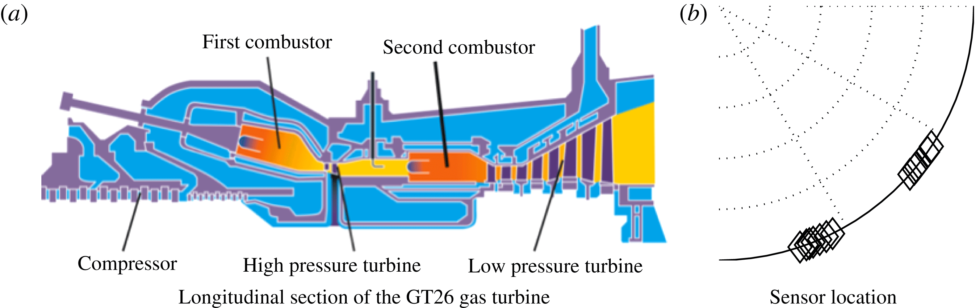
To validate the theory, we analyse the pulsation data of two tests of the Ansaldo GT26 engine before and after the installation of a set of acoustic dampers, at the same operating conditions. We present in figure 1(a) a sketch of the longitudinal section of the engine, showing a first annular combustor connected to a second annular sequential combustor through a high-pressure (HP) turbine. Güthe, Hellat & Flohr (Reference Güthe, Hellat and Flohr2009) discuss how sequential combustion systems operate compared with conventional systems with only one combustor. This paper focuses on the second combustor, which has inlet and outlet boundary conditions approximately choked, from now onwards referred to simply as the combustor. During the first test, the combustor exhibits a third-order
 $n=3$
azimuthal thermoacoustic mode that is linearly unstable and saturates nonlinearly to a stochastic attractor. Dampers are then installed in a second test. We use the pulsation data of the first test and the design of the dampers to predict the amplitude PDFs of the second test and compare them with the measurements.
(a) Sketch of the gas turbine. This paper discusses thermoacoustic instabilities in the second annular combustor only, referred to simply as the combustor, before and after the installation of
 $N_{d}=13$
Helmholtz resonators. (b) Zoom on a quarter of the cross section of the combustor showing the azimuthal location of the sensors (diamonds).

The fact that we first present the theory for an axial instability and then validate the theory for an azimuthal instability should not worry the reader. The formal analogies in the linear and nonlinear regimes of the low-order models of axial and azimuthal low-frequency instabilities were mentioned first by Crocco (Reference Crocco1969), and recently rediscussed by Ghirardo et al. (Reference Ghirardo, Juniper and Bothien2017). The validation on an azimuthal test case will actually shed light on the strength of the nonlinear interaction between azimuthal modes. The study of azimuthal thermoacoustic instabilities has been discussed in a stochastic framework by Noiray & Schuermans (Reference Noiray and Schuermans2013b ) with a simpler flame model, while similar equations discussing a rotational symmetric turbulent wake have been presented by Rigas et al. (Reference Rigas, Morgans, Brackston and Morrison2015), Brackston et al. (Reference Brackston, García de la Cruz, Wynn, Rigas and Morrison2016) and Rigas, Morgans & Morrison (Reference Rigas, Morgans and Morrison2017).
We need, however, an additional assumption regarding the flame model as compared with § 2.2. A thermoacoustic instability of azimuthal type has an acoustic velocity in the azimuthal direction that sweeps the flame in the transverse direction, i.e. orthogonally to the mean flow field through the burner (Fanaca et al. Reference Fanaca, Alemela, Hirsch and Sattelmayer2010; Hauser, Lorenz & Sattelmayer Reference Hauser, Lorenz and Sattelmayer2011). Under the assumption that the burners and the mean flow field close to the burner are rotationally symmetric, the effect on the heat release rate is zero in the linear regime, i.e. is only a nonlinear function of the azimuthal velocity amplitude. This has been observed experimentally (O’Connor & Acharya Reference O’Connor and Acharya2013; Saurabh et al. Reference Saurabh, Steinert, Moeck and Paschereit2014) and proved theoretically (Acharya, Shin & Lieuwen Reference Acharya, Shin and Lieuwen2013; Acharya & Lieuwen Reference Acharya and Lieuwen2014). Saurabh, Moeck & Paschereit (Reference Saurabh, Moeck and Paschereit2017) and Saurabh & Paschereit (Reference Saurabh and Paschereit2017) have shown that this effect is present at large amplitude of transverse velocity. If this nonlinear effect leads to a reduced heat release rate response, the nature of the azimuthal limit-cycle solution is found to change from a spinning to a standing solution (Ghirardo & Juniper Reference Ghirardo and Juniper2013). In the particular case at hand, the sequential burner is symmetrical with respect to the azimuthal direction, so that the effect can only be nonlinear. Existing numerical studies on this flame (Kulkarni et al. Reference Kulkarni, Bunkute, Biagioli, Duesing and Polifke2014; Yang et al. Reference Yang, Noiray, Scarpato, Schulz, Düsing and Bothien2015; Scarpato et al. Reference Scarpato, Zander, Kulkarni and Schuermans2016) have not specifically studied the dependence of the flame response to transverse acoustic excitation. We assume that this effect is not present and that the heat release rate model discussed in § 2.2 is valid.
In § 3.1, we discuss the reconstruction of the two azimuthal thermoacoustic modes. In § 3.2, the configuration of the dampers is presented and we justify why we study the two modes separately. In § 3.3, we discuss the pulsation amplitude statistics and compare them with the theoretical prediction.
3.1 Azimuthal mode reconstruction
To avoid systematic errors, we use only sensors of the same type, with the same microphone holder design and that were acquired through the same acquisition chain. Details of the sensors are discussed by Singla, Noiray & Schuermans (Reference Singla, Noiray and Schuermans2012) and their azimuthal positions are sketched in figure 1(b). Some sensors are located at the same azimuthal position but slightly different axial position and overlap in the figure. A first study ascertained that the different axial locations of the sensors do not reflect in different amplitudes of pulsation at this frequency. We then conclude that as a first approximation the mode amplitude is constant in the axial direction. In the azimuthal direction, the farthest two sensors span
 ${\approx}0.66$
rad. This distance is sufficient to reconstruct an
 $n=3$
azimuthal mode because a quarter wave of the mode spans a smaller angle,
 $2\unicode[STIX]{x03C0}/4n\approx 0.53$
rad.
The pressure field is written as the sum of two modes with amplitudes
 $\dot{\unicode[STIX]{x1D702}}_{1}(t)$
and
 $\dot{\unicode[STIX]{x1D702}}_{2}(t)$
,
 $$\begin{eqnarray}\displaystyle p(\boldsymbol{x},t)=\dot{\unicode[STIX]{x1D702}}_{1}\unicode[STIX]{x1D713}_{1}(\boldsymbol{x})+\dot{\unicode[STIX]{x1D702}}_{2}\unicode[STIX]{x1D713}_{2}(\boldsymbol{x}). & & \displaystyle\end{eqnarray}$$
We choose the two modes to be real valued and orthogonal, and such that their maximum value in the azimuthal direction at the axial coordinate of the burners is 1. This leads to two standing modes, such that one mode has the pressure antinodes where the other has the pressure nodes. We choose to study the pressure field as the sum of two standing waves with pressure nodes and antinodes fixed in space, albeit one can also carry out the study in terms of two counter-rotating spinning waves. At the burner outlet, the pressure field is
 $$\begin{eqnarray}\displaystyle p(\unicode[STIX]{x1D703},t) & = & \displaystyle \dot{\unicode[STIX]{x1D702}}_{1}(t)\cos (3\unicode[STIX]{x1D703}-\unicode[STIX]{x1D6FF})+\dot{\unicode[STIX]{x1D702}}_{2}(t)\sin (3\unicode[STIX]{x1D703}-\unicode[STIX]{x1D6FF}),\end{eqnarray}$$
 $$\begin{eqnarray}\displaystyle p_{k}(t) & = & \displaystyle p(t,\unicode[STIX]{x1D703}_{k})\quad k=1,2,\ldots ,N_{sensors},\end{eqnarray}$$
 $\unicode[STIX]{x1D6FF}$
is the orientation angle of the two modes and
 $n=3$
is the azimuthal order of the instability. The temporal evolution of the instantaneous values of the pressure amplitudes
 $\dot{\unicode[STIX]{x1D702}}_{1}(t)$
and
 $\dot{\unicode[STIX]{x1D702}}_{2}(t)$
determines whether the whole pressure field
 $p(t,\unicode[STIX]{x1D703})$
is a standing wave, a spinning wave or a mix of both types of mode at each instant of time. This aspect is discussed in detail by Ghirardo et al. (Reference Ghirardo, Juniper and Moeck2016) for a symmetric combustor without accounting for the background noise. We, however, focus here only on the amplitudes of the individual modes,
 $\dot{\unicode[STIX]{x1D702}}_{j}(t)$
.
To extract the values
 $\dot{\unicode[STIX]{x1D702}}_{j}(t),j=1,2$
, from the pressure readings
 $p_{k}(t)$
, we apply a multi-microphone method in the azimuthal direction and solve the overdetermined system (3.2b
) for
 $\dot{\unicode[STIX]{x1D702}}_{1,2}(t)$
in a least-squares sense (Seybert & Ross Reference Seybert and Ross1977; Åbom Reference Åbom1992). We do so for
 $\unicode[STIX]{x1D6FF}=0$
in a first step, and, in a second step, we calculate with a singular value decomposition the value of
 $\unicode[STIX]{x1D6FF}$
that minimizes the cross-correlation between the two time series
 $\dot{\unicode[STIX]{x1D702}}_{1}(t)$
and
 $\dot{\unicode[STIX]{x1D702}}_{2}(t)$
. The two modes, shaped like
 $\cos (n\unicode[STIX]{x1D703})$
and
 $\sin (n\unicode[STIX]{x1D703})$
in the frame of reference with the origin at
 $\unicode[STIX]{x1D703}=\unicode[STIX]{x1D6FF}$
, correspond to the two singular values of the singular value decomposition. In particular,
 $\unicode[STIX]{x1D6FF}$
is the angle for which the mode shaped like
 $\cos (n\unicode[STIX]{x1D703})$
has the largest amount of energy and the other mode shaped like
 $\sin (n\unicode[STIX]{x1D703})$
has the least amount of energy. The two modes before the installation of the dampers were rather close in frequency, with
 $$\begin{eqnarray}\displaystyle \unicode[STIX]{x0394}f_{ndim}\equiv \frac{|f_{1}-f_{2}|}{(f_{1}+f_{2})/2}\approx 9.52\times 10^{-4}, & & \displaystyle\end{eqnarray}$$
consistent with the assumed approximate rotational symmetry of the system before the installation of the dampers. After the installation of the dampers, the mean frequency of oscillation
 $(f_{1}+f_{2})/2$
was less than 2 % off from the value before their installation, and the two modes were slightly off in frequency, but not significantly, with
 $\unicode[STIX]{x0394}f_{ndim}\approx 1.49\times 10^{-2}$
. We assume that these differences are negligible, and approximate the oscillation frequency
 $f$
of the modes before and after the installation of the dampers with the mean frequency before their installation, and refer to this as the oscillation frequency in the following. We present results in non-dimensional units, by first applying a change of time variable so that the frequency
 $\unicode[STIX]{x1D714}=2\unicode[STIX]{x03C0}f$
becomes unity. We rescale the amplitudes by a fixed factor because we cannot disclose the physical values of pulsation.
3.2 Governing equations
This subsection briefly recalls the governing equations for two degenerate azimuthal modes in a rotationally symmetric combustor with a discrete number of flames. We motivate why it is convenient and reasonable to model each mode separately and then discuss how the installation of the dampers affects the equations.
The combustion chamber consists of
 $N_{s}=24$
sectors, with one flame in each sector. The equations for the two azimuthal modes before the installation of the dampers are
 $$\begin{eqnarray}\displaystyle \ddot{\unicode[STIX]{x1D702}}_{1}+\unicode[STIX]{x1D714}_{0}^{2}\unicode[STIX]{x1D702}_{1} & = & \displaystyle \mathop{\sum }_{j=1}^{N_{s}}{\mathcal{Q}}_{pr}[\dot{\unicode[STIX]{x1D702}}_{1}c_{j}+\dot{\unicode[STIX]{x1D702}}_{2}s_{j}]c_{j}-\unicode[STIX]{x1D6FC}\dot{\unicode[STIX]{x1D702}}_{1}+\unicode[STIX]{x1D70E}\unicode[STIX]{x1D709}_{1},\end{eqnarray}$$
 $$\begin{eqnarray}\displaystyle \ddot{\unicode[STIX]{x1D702}}_{2}+\unicode[STIX]{x1D714}_{0}^{2}\unicode[STIX]{x1D702}_{2} & = & \displaystyle \mathop{\sum }_{j=1}^{N_{s}}{\mathcal{Q}}_{pr}[\dot{\unicode[STIX]{x1D702}}_{1}c_{j}+\dot{\unicode[STIX]{x1D702}}_{2}s_{j}]s_{j}-\unicode[STIX]{x1D6FC}\dot{\unicode[STIX]{x1D702}}_{2}+\unicode[STIX]{x1D70E}\unicode[STIX]{x1D709}_{2},\end{eqnarray}$$
 $c_{j}=\cos (n\unicode[STIX]{x1D703}_{j})$
and
 $s_{j}=\sin (n\unicode[STIX]{x1D703}_{j})$
, with
 $\unicode[STIX]{x1D703}_{j}$
being the azimuthal positions of the
 $N_{s}=24$
sectors, and
 $n=3$
is the order of the azimuthal instability. Equations (3.4) are the equivalent of (2.30) for a rotationally symmetric annular system. They can be obtained by applying the same method as discussed in §§ 2.4–2.6, by accounting for two dominant degenerate modes
 $\unicode[STIX]{x1D713}_{1,2}$
instead of one and exploiting the fact that they are orthogonal.
One can, in principle, proceed similarly to § 2, apply temporal averaging and consider the corresponding Fokker–Planck equation for the coupled oscillators. However, we do not have an analytical nonlinear deterministic solution that extends the work of Ghirardo et al. (Reference Ghirardo, Juniper and Moeck2016) to non-rotationally symmetric systems, or an analytical solution for the resulting Fokker–Planck equations when stochastic noise is considered. The difficulty in expressing this solution arises because the equations depend now on three variables, the two amplitudes and the phase between the two oscillators. However, we notice that the interaction between the modes is only nonlinear, i.e. absent in the linear regime (Schuermans et al. Reference Schuermans, Paschereit and Monkewitz2006, p. 8), and then weaker than the response of each oscillator to itself. We then decide to ignore this interaction, leading to an uncoupled equation for each mode. We will discuss this hypothesis further in § 3.4.
After the first test,
 $N_{d}=13$
multivolume Helmholtz resonators with the same design are installed in the combustion chamber. Each damper is placed on the combustor walls, and azimuthally in the middle of each sector, like the burners. The contribution to the dynamics of each damper is described by (2.41) and (2.42). We assume that the mode shape is not substantially affected by the addition of the dampers. A posteriori, this is in line with the finding in § 3.1 that the frequencies of the two modes are indeed negligibly affected, suggesting that the same applies to the mode shapes too. This is also consistent with previous studies on industrial combustors, where the frequency was not affected by the addition of Helmholtz dampers (Bellucci et al.
Reference Bellucci, Flohr, Paschereit and Magni2004, Reference Bellucci, Schuermans, Nowak, Flohr and Paschereit2005). We, however, point out that the mode shape can be affected by the addition of the dampers. For example, Helmholtz dampers with a much larger size, not representative of industrial configurations, can lead to a significant change of the acoustic mode shape (Zahn et al.
Reference Zahn, Schulze, Hirsch and Sattelmayer2016, figure 14).
The admittance
 $Y$
appearing in (2.42) is then calculated at the oscillating frequency of the first test and is modelled accounting for the nonlinear amplitude response, the mean bias flow through the neck and the acoustic end corrections (Bellucci et al.
Reference Bellucci, Flohr, Paschereit and Magni2004; Bellucci Reference Bellucci2009). The damper design is not discussed in detail here because it does not constitute an element of novelty as compared with the existing literature. We refer the reader to Bothien et al. (Reference Bothien, Noiray and Schuermans2013) and Bothien & Wassmer (Reference Bothien and Wassmer2015), where the methodology is discussed and tested in the linear and nonlinear regimes on experimentally measured reflection coefficients of dampers mounted on impedance tubes.
Since the mode shape is constant in the axial and radial directions, both modes have the same value at the flame and at the damper neck in each sector, i.e.
 $\dot{\unicode[STIX]{x1D702}}_{1}c_{j}$
and
 $\dot{\unicode[STIX]{x1D702}}_{2}s_{j}$
respectively for the two modes at the
 $j$
th damper. This means that the argument of
 ${\mathcal{Y}}_{pr}$
in (2.41) is
 $\dot{\unicode[STIX]{x1D702}}_{1}c_{j}$
or
 $\dot{\unicode[STIX]{x1D702}}_{2}s_{j}$
, while the term
 $\unicode[STIX]{x1D713}(\boldsymbol{x}_{d})$
outside the square brackets is
 $c_{j}$
or
 $s_{j}$
, depending on whether we are considering the equation for
 $\{\dot{\unicode[STIX]{x1D702}}_{1},\unicode[STIX]{x1D713}_{1}\}$
or
 $\{\dot{\unicode[STIX]{x1D702}}_{2},\unicode[STIX]{x1D713}_{2}\}$
. We then consider the equation for the first mode, and notice that after the installation of the dampers there is an extra term in the equations which is the contribution of the changed boundary conditions at the damper necks. In particular, there is an extra term like (2.41) for each of the dampers in (3.4a
),
 $$\begin{eqnarray}\displaystyle \ddot{\unicode[STIX]{x1D702}}_{1}+\unicode[STIX]{x1D714}_{0}^{2}\unicode[STIX]{x1D702}_{1} & = & \displaystyle {\mathcal{S}}[\dot{\unicode[STIX]{x1D702}}_{1}]+\unicode[STIX]{x1D70E}\unicode[STIX]{x1D709}_{1},\end{eqnarray}$$
 $$\begin{eqnarray}\displaystyle {\mathcal{S}}[\dot{\unicode[STIX]{x1D702}}_{1}] & = & \displaystyle \mathop{\sum }_{j=1}^{N_{s}}{\mathcal{Q}}_{pr}\left[\dot{\unicode[STIX]{x1D702}}_{1}c_{j}\right]c_{j}-\unicode[STIX]{x1D6FC}\dot{\unicode[STIX]{x1D702}}_{1}+\mathop{\sum }_{k}{\mathcal{Y}}_{pr}\left[\dot{\unicode[STIX]{x1D702}}c_{k}\right]c_{k},\end{eqnarray}$$
 $k$
is summed only over the sectors where the dampers are mounted, and a second equation for the other azimuthal mode follows similarly. One observes trivially that dampers positioned where the coefficient
 $c_{k}=\cos (n\unicode[STIX]{x1D703}_{k})$
is small or zero have little or no damping effect. We choose to orient the frame of reference so that one of the two modes is maximally damped by the last summation term in (3.5b
) and the other oscillator is the least damped. The two modes are differently damped because the azimuthal pattern of the Helmholtz dampers is not uniform, i.e. some sectors have a Helmholtz damper and some others do not. In this optimal frame of reference, the orientation of the least damped mode is presented in figure 2(a).
(a) Positions of the pressure antinodes of only one of the two standing modes that we decompose the pressure field in (the other mode is rotated by
 $\unicode[STIX]{x03C0}/6$
). The mode with the largest amplitude reconstructed from the time series (squares) and the mode predicted to be least damped (crosses) have approximately the same orientation. (b) Damping functions
 $F^{\sharp }(A)$
characterizing the effects of the dampers on each of the two modes, in the linear approximation (dashed lines) and the fully nonlinear (continuous lines) case. The damping functions are different for the two modes because the azimuthal pattern of the dampers is not uniform. The quantity
 $\lim _{A\rightarrow 0^{+}}-F^{\sharp }(A)/A$
is the linear deterministic growth rate reduction gained by the application of the dampers on each mode, respectively 3 % and 4.8 % of
 $2\unicode[STIX]{x03C0}f$
for the least and most damped modes.

Finally, the extra terms described in (2.42) for the two azimuthal modes are
 $$\begin{eqnarray}\displaystyle F_{c}^{\sharp }(A) & = & \displaystyle \mathop{\sum }_{k=1}^{N_{d}}\frac{1}{2}\,\text{Re}[Y_{pr}[A|c_{k}|]]Ac_{k}^{2},\end{eqnarray}$$
 $$\begin{eqnarray}\displaystyle F_{s}^{\sharp }(A) & = & \displaystyle \mathop{\sum }_{k=1}^{N_{d}}\frac{1}{2}\,\text{Re}[Y_{pr}[A|s_{k}|]]As_{k}^{2}.\end{eqnarray}$$
First test case, before damper installation. (a) Estimated PDFs of the acoustic pressure amplitudes
 $A_{1}$
and
 $A_{2}$
of the two azimuthal modes. The two PDFs are rather close, consistent with the system being axisymmetric before the damper installation. The vertical dot-dashed and dashed lines are the mean and 98th percentile values of the PDF. We present in (b,c) with black dots the histograms of the processes
 $A_{1}\dot{\unicode[STIX]{x1D711}}_{1}$
(b) and
 $A_{2}\dot{\unicode[STIX]{x1D711}}_{2}$
(c). The magenta lines are the normal distributions with estimated standard deviation
 $\unicode[STIX]{x1D70E}/\sqrt{2}$
that best fit the histograms.

3.3 Amplitude statistics
Each of the two azimuthal modes
 $\dot{\unicode[STIX]{x1D702}}_{j}$
is treated as a stationary ergodic process (Lin Reference Lin1967). We reasonably assume stationarity because the engine was operated at fixed conditions during the acoustic pressure time series acquisition, and we then expect the statistics of the process to not change over time. We assume ergodicity so that we can estimate the statistical moments
 $E[\dot{\unicode[STIX]{x1D702}}_{j}^{n}P(\dot{\unicode[STIX]{x1D702}}_{j})]$
of the process from the time averages of the moments of a sufficiently long time series. We tested this by carrying out a statistical bootstrapping procedure on the statistics discussed in this section, showing very good convergence of the estimated PDF. We note that it is harder to obtain convergence for cases like transients and the occurrence of strong pulsations over a observation time that is very short because of the danger of structural damage in the engine/experiment. Moreover, noisy systems that would be stable but exhibit bursts of oscillations with intermittent behaviour (Kabiraj et al.
Reference Kabiraj, Saurabh, Wahi and Sujith2012; Kabiraj & Sujith Reference Kabiraj and Sujith2012) when noise is considered are a challenge. The signals
 $\dot{\unicode[STIX]{x1D702}}_{j}$
are band pass filtered in the range
 $[3\unicode[STIX]{x1D714}/4,5\unicode[STIX]{x1D714}/4]$
to isolate the oscillating mode. The analytic signals are calculated and from them the slowly varying amplitudes
 $A_{j}(t)$
and slowly varying phases
 $\unicode[STIX]{x1D711}_{j}(t)$
are extracted. We then apply kernel density estimation (Botev, Grotowski & Kroese Reference Botev, Grotowski and Kroese2010) on the statistical sample
 $\{A_{j,n},n=1,2,\ldots ,N\}$
and present the two estimated PDFs in figure 3(a). The application of bootstrapping on the sample population revealed negligible deviations from the PDFs, so that we conclude that the time series are long enough to guarantee good convergence. For each PDF of figure 3(a), we plot with vertical lines the mean value
 $E(A)$
and the 98 % percentile value. These values characterize respectively the level of average pulsation and the level of rare pulsation, which are useful for industrial applications.
We present in figure 3(b) with black dots the histogram of the two processes
 $A_{1}\dot{\unicode[STIX]{x1D711}}_{1}$
and
 $A_{2}\dot{\unicode[STIX]{x1D711}}_{2}$
with a bin size that is optimal, as discussed by Shimazaki & Shinomoto (Reference Shimazaki and Shinomoto2007), together with the normal distribution that best fits the histogram points in a least-squares sense. The identified standard deviations
 $\unicode[STIX]{x1D70E}_{1}/\sqrt{2}$
and
 $\unicode[STIX]{x1D70E}_{2}/\sqrt{2}$
of the two distributions are then used in (2.40) to calculate
 $F_{1}(A)$
and
 $F_{2}(A)$
.
The two sets of objects
 $\{F_{1}(A),\unicode[STIX]{x1D70E}_{1}\}$
and
 $\{F_{2}(A),\unicode[STIX]{x1D70E}_{2}\}$
presented in figure 3 characterize the state of the system before damper installation and are very similar, suggesting rotational symmetry of the system in the first test, often assumed in low-order models of azimuthal instabilities. Ideally, we would like to have only one set
 $\{F(A),\unicode[STIX]{x1D70E}\}$
describing the state of the system in the first test, and then use (2.43) on this state with each of the two damping functions
 $F^{\sharp }(A)$
presented in figure 2(b) to predict the amplitude of each of the two modes after damper installation in the second test. Since it is hard to decide how one would best average the two sets, we prefer to make two predictions, each based individually on one of the two sets. We present in figure 4(a) the comparison of the two predicted
 $P(A)$
curves for the least damped mode with the measurements. The installation of the dampers leads to a significant reduction of pulsation amplitudes. The agreement of the PDFs between the two predictions and the measurements is good. The predicted integral quantities of the PDFs, i.e. the mean values (dash-dotted lines) and the 98th percentile values (dashed lines), have in the worst case 30 % accuracy and overpredict the measured ones, suggesting that the damper design is conservative.
After damper installation, observed in the optimal frame of reference. (a) Comparison between predictions (grey) and measurement (black) for the more damped mode. The line styles have the same legend as figure 3(a). We find a slight overprediction of the predictions compared with the measurements in terms of PDFs, mean values and 98th percentile values. (b) The same as (a) for the least damped mode, which is oriented as in figure 2(a). The blue and red colours correspond to the lines of figure 2(b).

The same method was applied also to a second test case, based on another two comparable time series before and after the damper addition. This second test case was at different operating conditions from the first test case presented in figures 3 and 4. The amplitudes of pulsation before damper installation are presented in figure 5(a). Compared with the first test case in figure 3(a), the two azimuthal modes oscillate at a smaller amplitude and the two PDFs differ quantitatively between each other, implying that the system is less rotationally symmetric in this second test case. Nonetheless, we find that after the damper installation, the reconstructed mode orientation matches the predicted orientation. The orientation figure is very similar to the one presented in figure 2(b) and is thus not reported. The comparison of the predicted amplitudes with the measured amplitudes after the damper installation is presented in figure 5(b,c). The maximum error drops to 13 %.
This is the first time that a comparison between predictions and measurements of PDFs of acoustic pressure amplitudes has been presented in thermoacoustics, and we believe that this level of accuracy is still remarkable. In particular, the predicted shape of the distribution resembles strongly the measured one in both test cases, and in each test case, the error is similar between the least and most damped modes. Among the factors that may contribute to a systematic overprediction, we mention that the second test was carried out at an operating mean pressure in the combustion chamber that was a few per cent off from the first test. Another possible reason relates to the saturation of the damper response in the nonlinear regime. A gentler saturation would lead to steeper functions
 $F^{\sharp }$
in figure 2(b) and ultimately to lower predicted amplitudes.
Second test case. (a) The PDFs of the two azimuthal modes before the damper installation. (b) Comparison between predictions (blue) and measurements (black) for the more damped azimuthal mode. The line styles have the same legend as figure 3(a). We find quite a good agreement between predictions and measurements in terms of PDFs, mean values and 98th percentile values. (c) The same as (b) but for the least damped azimuthal mode.

3.4 Weak interaction of the two modes
Upon request of a referee, we further discuss the nonlinear interaction between the two azimuthal modes. We consider the case presented in figure 4, where the system is asymmetric, i.e. after damper installation. We present in figure 6 the joint PDF (JPDF)
 $P_{\{A,B\}}(A,B)$
, similarly to previous studies (Noiray & Schuermans Reference Noiray and Schuermans2013b
; Worth & Dawson Reference Worth and Dawson2013). We present in figure 6(b) the product of the two marginal PDFs
 $P(A)$
and
 $P(B)$
of the two processes (black lines of figure 4). This product would be the JPDF of the system in the case where the two processes
 $A$
and
 $B$
were independent. We present in figure 6(c) the difference between the two bidimensional functions and observe how the two functions are really close. There is no clear pattern in the difference between the two, and the non-exact match can probably be attributed to the fine grid size of the histogram compared with the time series length. This suggests that the JPDF of figure 6(a) is indeed factorable, i.e. can be expressed in terms of the marginal PDFs as in figure 6(b). We cannot, however, take this evidence to imply that the two processes are independent, because the factorability of the JPDF of two processes as the product of the marginal PDFs of the two is only a necessary condition for the independence of the processes (it is also sufficient in the case where one considers two random variables instead of two stochastic processes). Indeed, we know that a thorough independence test of the two processes would prove them not to be independent, because of the nonlinear interaction in (3.4). We can, however, take figure 6 as additional evidence that the interaction between the two azimuthal modes is indeed weak. This suggests that the marginal PDFs of the amplitudes of the two azimuthal modes can be characterized by a model where such interaction is neglected, as done in this paper.
Factorability of the JPDF of the test case of figure 4. (a) The JPDF of the two-dimensional stochastic process
 $\{A,B\}$
, estimated with a
 $50\times 50$
bidimensional histogram. (b) The product of the two marginal PDFs of the two processes
 $A$
and
 $B$
. (c) The difference between (a) and (b): no clear pattern is observed in the error, suggesting that the JPDF is indeed factorable.

4 Conclusions
We study thermoacoustic instabilities where only one dominant frequency of oscillation is excited in the system and with a zero-Mach-number assumption, which is reasonable in land-based gas turbine combustors. In particular, we model the thermoacoustic oscillation with one Galerkin mode, neglecting the change in the mode shape due to the flame response. We model the heat release rate fluctuations coming from the flame as the sum of a deterministic and a stochastic component. The deterministic component is a nonlinear time-invariant operator of the acoustic pressure at the flame location in the time domain, then mapped to a describing function in the frequency domain. The stochastic component is the background combustion noise that is present regardless of the acoustic excitation of the flame and is modelled as an additive white Gaussian stochastic process. From the governing equations, we obtain a Galerkin series that accounts for spatially varying temperature and density fields. We treat the thermoacoustic equations as a weak perturbation of the fluctuating pressure equation and truncate the Galerkin series to a single-mode approximation. We obtain a single oscillator model governing the acoustic pressure amplitude of the perturbed Galerkin mode. In the oscillator equations, the heat release rate appears directly in the equations, as opposed to the current literature where its time derivative usually appears. We show how one can predict the probability density functions (PDFs) of the acoustic pressure amplitude, and also recover the projected describing function driving the instability, from experimental time series of a self-excited combustor. We show that the linear growth rates of the system when noise is not considered are hard to estimate from time series data based on mathematical and physical arguments. We show also that linear growth rates are less representative of the nonlinear state of the stochastic system compared with the case of deterministic systems, where noise is absent.
The theory is then tested on an azimuthal thermoacoustic instability in a full scale annular combustor, under the assumption that the interaction between the two azimuthal modes is negligible because it is only a nonlinear effect. We measure the state of the system before the installation of a set of Helmholtz resonators and then make a prediction accounting for the response of the dampers in the linear and nonlinear regimes, assuming that only the orientation of the thermoacoustic modes, and not their shape, is affected by the dampers. We find good agreement between predictions and measurements, in terms of both the orientation of the azimuthal modes and the PDFs. This suggests that the nonlinear interaction between the two modes may indeed be neglected for the purpose of amplitude prediction. Numerical simulations of stochastic low-order models can further substantiate this experimental finding on the strength of this nonlinear interaction.
Future work should focus on a heat release rate model that is able to capture the effect of transients. In the simplest case, the heat release rate response model that captures this effect would depend on the acoustic pressure or velocity only via a delay operator. Crawford, Verriest & Lieuwen (Reference Crawford, Verriest and Lieuwen2013) predict the statistics of an oscillator forced by a delayed term and Gaussian noise, but in the linear regime only. Ghirardo et al. (Reference Ghirardo, Juniper and Bothien2017) discuss the effect of a delayed flame response on the system in the nonlinear regime, but do not discuss the effect of additive white Gaussian noise. There is a need to study the effect of this delay in the nonlinear regime and accounting for additive white Gaussian noise. The theoretical prediction of exact statistics of self-excited oscillations with a delayed forcing term may prove difficult, but the strength of this effect on selected points of the parameter space should be reasonably easy to investigate numerically.
Appendix A. Choice of boundary conditions for the Galerkin modes
In § 2.3, we impose that
 $\unicode[STIX]{x1D735}\unicode[STIX]{x1D713}\boldsymbol{\cdot }\boldsymbol{n}=0$
on the boundary
 $\unicode[STIX]{x2202}\unicode[STIX]{x1D6FA}$
. This matches the boundary condition of the original problem (2.3) on the wall of the combustor, but does not match the boundary conditions at the inlet and outlet.
The boundary conditions are usually chosen such that the homogeneous problem in § 2.3 is self-adjoint, and then the resulting eigenmodes
 $\{\unicode[STIX]{x1D713}_{n}\}$
are orthogonal and can used as a basis. Morse & Feshback (Reference Morse and Feshback1953b
, § 9.2) showed that a sufficient condition to do so is to choose Dirichlet or Neumann boundary conditions on the boundary
 $\unicode[STIX]{x2202}\unicode[STIX]{x1D6FA}$
. Nicoud et al. (Reference Nicoud, Benoit, Sensiau and Poinsot2007, Appendix B, equation (B8)) more recently pointed out that the choice of a complex reduced impedance
 $Z=\text{i}R_{0}\unicode[STIX]{x1D714},R_{0}\in \mathbb{R}$
, also guarantees orthogonal eigenmodes. One chooses among these options the one that best resembles the boundary condition of the original problem. On the walls of the combustor, the choice is trivial, because Neumann boundary conditions match the boundary conditions of the problem exactly. At the inlet and the outlet of the domain, the choice depends on the actual boundary conditions of the problem at hand. Taking the Fourier transform of (2.4), and substituting on the left-hand side the expression for
 $\hat{\boldsymbol{u}}_{1}$
from the Fourier transform of (2.3b
) and on the right-hand side
 $u_{\bot }={\mathcal{Y}}p$
with
 ${\mathcal{Y}}$
defined in (2.5), we obtain
 $$\begin{eqnarray}\displaystyle \frac{-\unicode[STIX]{x1D735}\hat{p}_{1}\boldsymbol{\cdot }\boldsymbol{n}}{\unicode[STIX]{x1D70C}\text{i}\unicode[STIX]{x1D714}}=-\frac{{\mathcal{R}}-1}{{\mathcal{R}}+1}\frac{\hat{p}}{\unicode[STIX]{x1D70C}_{0}c}. & & \displaystyle\end{eqnarray}$$
Multiplying both sides by
 $\unicode[STIX]{x1D70C}_{0}i\unicode[STIX]{x1D714}$
and moving the terms, we obtain
 $$\begin{eqnarray}\displaystyle \unicode[STIX]{x1D735}\hat{p}_{1}\boldsymbol{\cdot }\boldsymbol{n}+\text{i}\frac{1-{\mathcal{R}}}{1+{\mathcal{R}}}k\hat{p}_{1}=0, & & \displaystyle\end{eqnarray}$$
where we have introduced the wavenumber
 $k=\unicode[STIX]{x1D714}/c$
. This expression matches equation (9.2.1) of Morse & Feshback (Reference Morse and Feshback1953b
),
 $$\begin{eqnarray}\displaystyle \unicode[STIX]{x1D735}\hat{p}_{1}\boldsymbol{\cdot }\boldsymbol{n}+f\hat{p}_{1}=0, & & \displaystyle\end{eqnarray}$$
where
 $f\equiv \text{i}((1-{\mathcal{R}})/(1+{\mathcal{R}}))k$
. We observe that the absolute value of the factor
 $f$
depends on the value of the reflection coefficient on the boundary and the wavenumber
 $k$
. For the application of this paper,
 ${\mathcal{R}}$
is very close to unity because the flow field is close to choked (Marble & Candel Reference Marble and Candel1977), and
 $f$
is small. It follows that (A 3) is a perturbation of the Neumann boundary condition
 $\unicode[STIX]{x1D735}\hat{p}_{1}\boldsymbol{\cdot }\boldsymbol{n}=0$
, which is then chosen as the boundary condition for the homogeneous problem. For
 $f$
large, one would instead impose Dirichlet boundary conditions. We refer the reader to Morse & Feshback (Reference Morse and Feshback1953b
, § 9.2) for a discussion of the convergence rate of either option. A discussion of how a linear combination of Galerkin modes can approximate the solution, despite the fact that each Galerkin mode does not respect the actual boundary condition, can be found in Culick (Reference Culick2006, Annex F).