


1. Introduction
Traditional auto insurance ratemaking relies primarily on static driver and vehicle characteristics, which are typically evaluated at discrete points in time (e.g., annually). Accordingly, pricing is typically conducted at the driver level and remains largely static over time. These covariates are informative for grouping drivers into classes within which the inherent risk is assumed to be relatively homogeneous. However, substantial heterogeneity may still remain among drivers even in the same group. Since such covariates do not directly reflect trip-level driving styles or dynamic driving environment, they are limited in their ability to capture heterogeneity arising from differences in individual behavioral risk.
With recent technological advances enabling high-frequency data collection, telematics has emerged as a means to address the limitations of traditional ratemaking. This shift supports behavior-derived risk assessment and can provide inputs for usage-based insurance (UBI) frameworks, provided that the resulting behavioral measures are validated against external outcomes such as claims or collisions. In this context, telematics signals are used to refine risk prediction by directly measuring how a vehicle is operated at high temporal resolution. Their value lies in providing a behavior-derived basis for reducing the remaining heterogeneity among policyholders and, consequently, for improving actuarial fairness. When traditional covariates leave residual heterogeneity within rating groups, a telematics-based behavioral risk index can support a pay-how-you-drive perspective by aligning risk assessment more closely with realized driving behavior. This data-driven orientation is important for fairness because it shifts the risk assessment toward observed driving behavior and away from indirect proxy covariates, while still requiring future validation against claim outcomes and contextual driving information before being used directly for ratemaking.
The actuarial telematics literature has rapidly evolved, providing a variety of methods to manage this rich information for insurance applications. The first strand focuses on “representation and feature construction” to turn high-frequency driving records into actuarial covariates. This includes early work that constructs telematics observables at multiple driving scales for individualized risk pricing (Weidner et al. Reference Weidner, Transchel and Weidner2016), covariate selection and engineered summaries from telematics signals (Wüthrich Reference Wüthrich2017), low-dimensional representations such as speed–acceleration heatmaps and related feature extraction frameworks (Gao and Wüthrich Reference Gao and Wüthrich2018; Gao et al. Reference Gao, Meng and Wüthrich2019), as well as broader data mining approaches that uncover common driving patterns from telematics records (Chan et al. Reference Chan, Tseung, Badescu and Lin2025b). The second strand develops “actuarial modeling and pricing frameworks” that incorporate telematics information into insurance models and rating systems, ranging from credibility-style multivariate formulations and model-based integration (Denuit et al. Reference Denuit, Guillén and Trufin2019), to assessments of the incremental value of dynamic telematics updates (Henckaerts and Antonio Reference Henckaerts and Antonio2022), bonus–malus style scoring for sequential ratemaking (Yáñez et al. Reference Yáñez, Guillén and Nielsen2025), as well as empirical studies on how telematics improves claims prediction and classification (Meng et al. Reference Meng, Wang, Shi and Gao2022; Duval et al. Reference Duval, Boucher and Pigeon2022; Duval et al. Reference Duval, Boucher and Pigeon2024). Many approaches essentially reduce high-frequency telematics time series to engineered features or summary statistics, but a large portion of the temporal structure in the signals has remained unexploited. This compression has limitations in detecting risk-relevant patterns that are localized in time. This motivated the third strand “driving dynamics and state evolution” that leverages the temporal structure of the signals by using sequential or latent state models to describe how risk-relevant behavior unfolds over time and how deviations from typical behavior can be identified (Meng et al. Reference Meng, Wang, Shi and Gao2022; Jiang and Shi Reference Jiang and Shi2024; Chan et al. Reference Chan, Badescu and Lin2025a). In particular, Chan et al. (Reference Chan, Badescu and Lin2025a) propose a multivariate Continuous-Time Hidden Markov Model (CTHMM) to model a trivariate response comprising speed, longitudinal acceleration, and lateral acceleration. They construct an anomaly index that quantifies the number of behavioral outliers observed during a trip.
Within this line of telematics research, a natural question arose: can behavioral risk be more informative if we also know how severe an observed behavioral pattern is? Most telematics-based risk assessments remain fundamentally frequency-oriented: those approaches primarily emphasize how often abnormal behavior occurs but pay comparatively limited attention to how severe those behaviors are. As a natural extension, this paper proposes to incorporate signal severity as an additional dimension to the telematics-based risk assessment.
In a conventional frequency–severity ratemaking study, “severity” usually refers to the loss amount conditional on a claim. In this paper, however, no claim size is being modeled. The severity is associated with the magnitude and rarity of a localized acceleration or braking pattern relative to a portfolio-anchored baseline distribution. After the signal is transformed into the multi-scale coefficient representation, large magnitude coefficients, which are produced by sharper localized acceleration or braking behavior, tend to lie farther in the tails. Values near the fitted Gaussian core are interpreted as typical patterns, whereas large magnitude values far into the left or right tail are interpreted as rarer and more severe behavioral deviations. Thus, severity is not an observed insurance loss outcome, but a signal-derived measure that combines the magnitude of a localized telematics pattern with its rarity relative to the portfolio baseline.
1.1. Data and preliminary analysis
This section describes the data that will be used in this paper and presents a preliminary analysis to justify the introduction of behavioral severity to risk assessment. The analysis shows how frequency-based summaries can miss important risk-relevant patterns and how severity-based summaries can help identify those patterns more accurately. This preliminary example motivates the proposed frequency–severity framework by illustrating why tail depth provides useful information beyond tail frequency.
1.1.1. Data
The UAH-DriveSet introduced by Romera et al. (Reference Romera, Bergasa and Arroyo2016) is a public smartphone-sensor dataset for driver behavior analysis. In this paper, we use the controlled dataset, which was recorded using the DriveSafe application. The dataset includes recordings from six different drivers with their own vehicles under three instructed behavioral states: normal, aggressive, and drowsy. Normal driving reflects typical everyday behavior, aggressive driving shows impatience and abrupt maneuvers such as overspeeding or tailgating, and drowsy driving simulates mild sleepiness with occasional inattention.
Data were collected on two prespecified routes near Alcalá de Henares in the Community of Madrid, Spain: a secondary road route and a motorway route. Each driver repeats these routes under the three instructed behavioral states, yielding 5 or 7 trips per driver on each road type. On the secondary road, each of Drivers 1–5 contributes four trips (normal1, normal2, aggressive, and drowsy), whereas on the motorway each driver contributes one trip per instructed state (normal, aggressive, drowsy). The only exception is Driver 6 who completes the motorway set but provides only normal and drowsy on the secondary road due to limited vehicle autonomy. Consequently, there are 40 trips, and each operated about 8–20 minutes. Table 1 summarizes the trips in the dataset. In this paper, we solely focus on longitudinal acceleration recorded at 10 Hz (every 0.1 seconds) in units of G (
 $9.8\,\mathrm{m/s^2}$
), where positive values indicate acceleration and negative values indicate braking. Since this controlled dataset has also been analyzed by Chan et al. (Reference Chan, Badescu and Lin2025a), it allows us to contrast the proposed frequency–severity framework with their frequency-oriented framework.
1.1.2. Preliminary analysis
For a comparison of the distributional profiles of different behavioral states, the empirical densities for longitudinal acceleration of Driver 1’s three motorway trips are displayed in Panel (a) in Figure 1. In the panel, we can see that normal and drowsy trips both concentrate near zero, and drowsy places even more mass around zero than normal. This illustrates the difficulty of identifying risk-relevant patterns of the drowsy or inattentive driving profile because it looks even safer than normal from a distributional perspective. In the following, we call this normal-looking profile. This normal-looking profile implies that risk-relevant differences may be hidden in the tails rather than in the bulk of the distribution, so there is a need to conduct a closer examination of the structural difference among the behavioral states by inspection of their tail behaviors.
Summary of the UAH-DriveSet controlled dataset: driver demographics, vehicle information, and the number of available trips by road type (secondary vs. motorway).

Table 1. Long description
The table presents data on six drivers, detailing their gender, age, vehicle, fuel type, and the number of trips made on secondary roads and motorways. The table has six rows and seven columns. Column headers are Driver, Gender, Age, Vehicle, Fuel, Sec. trips, Mot. trips, and Total. Row 1: Driver D1, Male, Age 40-50, Vehicle Audi Q5 (2014), Fuel Diesel, Sec. trips 4, Mot. trips 3, Total 7. Row 2: Driver D2, Male, Age 20-30, Vehicle Mercedes B180 (2013), Fuel Diesel, Sec. trips 4, Mot. trips 3, Total 7. Row 3: Driver D3, Male, Age 20-30, Vehicle Citroen C4 (2015), Fuel Diesel, Sec. trips 4, Mot. trips 3, Total 7. Row 4: Driver D4, Female, Age 30-40, Vehicle Kia Picanto (2004), Fuel Gasoline, Sec. trips 4, Mot. trips 3, Total 7. Row 5: Driver D5, Male, Age 30-40, Vehicle Opel Astra (2007), Fuel Gasoline, Sec. trips 4, Mot. trips 3, Total 7. Row 6: Driver D6, Male, Age 40-50, Vehicle Citroen C-Zero (2011), Fuel Electric, Sec. trips 2, Mot. trips 3, Total 5.
We apply simple quantile layers to examine the tail structure. These quantile layers here are only a descriptive proxy to illustrate tail depth, while later sections define the signal severity formally using our proposed framework. We compute the pooled lower tail quantiles based on the three trips and then commonly apply them to all the trips, as shown in Panel (b) in Figure 1. Specifically, we combine all acceleration observations across the trips into one sample and compute its
 $0.5\%$
,
 $0.1\%$
, and
 $0.05\%$
lower tail quantiles, denoted by
 $q_{0.5\%}$
,
 $q_{0.1\%}$
, and
 $q_{0.05\%}$
. Values below these thresholds represent increasingly extreme deceleration-relevant magnitude, and Table 2 reports the corresponding layer counts.
Driver 1 motorway example: counts of lower-tail observations in the pooled distribution, grouped into three severity layers defined by empirical left-tail quantiles (0.5%, 0.1%, and 0.05%).

Table 2. Long description
The table presents counts of lower-tail observations in a pooled distribution, grouped into three severity layers defined by empirical left-tail quantiles (0.5%, 0.1%, and 0.05%). It has three rows and four columns. The columns are labeled as Driving state, #(q0.1% < q ≤ q0.5%), #(q0.05% < q ≤ q0.1%), and #(q ≤ q0.05%). The row labels are Normal, Drowsy, and Aggressive. Row 1: Driving state, Normal; #(q0.1% < q ≤ q0.5%), 41; #(q0.05% < q ≤ q0.1%), 0; #(q ≤ q0.05%), 0. Row 2: Driving state, Drowsy; #(q0.1% < q ≤ q0.5%), 21; #(q0.05% < q ≤ q0.1%), 3; #(q ≤ q0.05%), 7. Row 3: Driving state, Aggressive; #(q0.1% < q ≤ q0.5%), 39; #(q0.05% < q ≤ q0.1%), 10; #(q ≤ q0.05%), 6.
Driver 1 motorway example: longitudinal acceleration densities (left) and trip trajectories with pooled left-tail thresholds marked at the 0.5%, 0.1%, and 0.05% quantiles (right).

The result shows that multiple depths in the tails carry information that frequency-based summaries can miss. For example, if one only counts exceedances beyond
 $q_{0.5\%}$
, normal would appear riskier than drowsy (the sum of exceedances is 41 vs.
 $21+3+7=31$
) from Table 2. In contrast, deeper layers reveal that drowsy places more mass in the extreme tail: drowsy has 3 exceedances in
 $(q_{0.05\%},q_{0.1\%}]$
and 7 exceedances below
 $q_{0.05\%}$
, while normal has none in either layer, which makes it separable once the severity-based summaries are taken into account.
This mechanism is consistent with the frequency-based approach in Chan et al. (Reference Chan, Badescu and Lin2025a), under which drowsy in the same controlled dataset was not flagged as risky by their CTHMM framework. In the same controlled dataset, Chan et al. (Reference Chan, Badescu and Lin2025a) report that the drowsy trip had a lower anomaly index than normal by their CTHMM framework. Our preliminary analysis helps explain why this can happen: the drowsy trip has fewer shallow exceedances than the normal trip, but it places more observations in deeper tail layers. Thus, the drowsy trip is not necessarily more frequent in abnormal behavior, but it is more severe in the tail-depth sense. This preliminary analysis provides concrete evidence that incorporating severity structure based on multiple tail layers enables a more refined evaluation of driving behavior in telematics signals. Therefore, this motivates the proposed frequency–severity joint behavioral risk index, whose overall signal-to-index construction is summarized in the “Methodology Overview” section before the technical details are introduced.
1.2. Methodology overview: from telematics signals to a behavioral risk index
The main idea of the framework is to convert a raw telematics signal into an interpretable measure of risky driving behavior. We first decompose the signal into wavelet-based components so that localized driving patterns, such as harsh acceleration or braking, can be detected at different time scales. We then pool the important signal coefficients across all trips to create a portfolio-level baseline and use this baseline to identify which patterns are rare and extreme. These extreme regions are interpreted as severity layers: the farther a coefficient lies in the tail, the more severe the driving pattern is. For each trip, we then count how often the signal falls into each severity layer. The final risk index is not just a count of extreme events; it gives more weight to rarer and more severe patterns so that a trip with fewer but very harsh events can be distinguished from a trip with many milder deviations. This signal-to-index construction is unsupervised with respect to insurance outcomes because it does not require claims or collisions. Instead, it evaluates behavioral risk directly from telematics signals, which is useful in practical settings where claims are sparse.
Overview of the proposed framework. Panel (a): how the telematics signal is transformed into a wavelet-based representation. Panel (b): the fitted severity model where the Gaussian component describes typical patterns, while Uniform layers represent increasingly extreme patterns. Panel (c): an example of trip-level index for each behavioral state and sequentially updated driver-level index.

Figure 2. Long description
The image contains three panels. Panel A: A line graph shows the transformation of a telematics signal into a wavelet-based coefficient series. The x-axis represents time, and the y-axis represents the signal. The graph illustrates the process of converting the telematics signal into finer and coarser scales using MODWT and across-level aggregation. Panel B: A density plot displays the portfolio severity baseline. The x-axis represents the coefficient, and the y-axis represents density. The plot shows typical behavior in the center with severity layers on either side, labeled as Lv2-, Lv1-, Lv1+, and Lv2+. Panel C: A bar and line graph combination shows the behavioral risk index. The x-axis represents different trips (normal1, drowsy, normal2, aggressive), and the y-axis represents the index. The bar graph shows the trip-level index, while the line graph shows the updated driver-level index, indicating how the index changes sequentially across trips.
The proposed framework integrates three components. The overview in Figure 2 shows the main structure of the framework before the details are introduced. It illustrates how a raw telematics signal is first transformed into a representation based on the signal’s pattern, how the retained coefficients define a portfolio severity baseline, and how the resulting layer-wise counts are converted into trip- and driver-level behavioral risk indices.
-
• Panel (a): Signal representation via wavelet transform. A telematics signal is transformed using the Maximal Overlap Discrete Wavelet Transform (MODWT) (Percival and Walden Reference Percival and Walden2013). The red wavelet filters in Panel (a) act as a moving local pattern detector. A filter that represents a particular time scale scans the signal at every available time point and produces large coefficients when the signal contains a harsh acceleration or braking pattern that stands out from its local background. Repeating this scan at multiple time scales allows the representation to capture both shorter and longer localized patterns that are detected by a finer and coarser filter, respectively. The coefficients from multiple scales are then aggregated into a single trip-level series that summarizes the multi-scale representation over the trip.
-
• Panel (b): Portfolio baseline and severity layers. Before constructing the portfolio baseline, the aggregated coefficient series is thinned to reduce the temporal dependence. The retained coefficients after thinning from all trips are then pooled to form a portfolio baseline. The central part of this baseline represents typical driving patterns, while the tails represent rare and extreme patterns. We fit a Gaussian–Uniform mixture model to this baseline, where Gaussian components fit the central part and Uniform components fit the tail regions. From an actuarial perspective, these Uniform components serve as severity layers, as shown in Panel (b): severity does not mean claim size here, but how rare and extreme a telematics pattern is relative to the portfolio baseline.
-
• Panel (c): Trip-level scoring and driver-level updating. For each trip, we count how often the coefficient series falls into each severity layer. The behavioral risk index combines these layer-wise counts with severity weights based on portfolio-level rarity, after normalizing by trip exposure, defined as the number of retained coefficients. Thus, a trip receives a higher index when the extreme pattern occurs more frequently or falls into more severe tail layers. Panel (c) illustrates how normal, aggressive, and drowsy can receive different trip-level indices and how the driver-level behavioral risk profile is sequentially updated.
In Sections 2–4, these three steps are formalized using the MODWT representation, a Gaussian–Uniform mixture model with multiple Uniform components, and a Poisson–Gamma conjugate model.
1.3. Practical value of the proposed index
The main goal of the proposed index is to provide a behavior-derived measure of driving risk without directly relying on claims or traditional rating covariates. In other words, the index recovers behavioral information from raw driving signals by converting high-frequency telematics signals into an interpretable numerical index.
This signal-to-risk view is closely connected to the scale-sensitive telematics perspective of Weidner et al. (Reference Weidner, Transchel and Weidner2016), who emphasize that risk-relevant information can appear at different degrees of granularity, ranging from maneuver-level behavior to segment-level, trip-level, and insurance-period summaries. Our framework adapts this principle through the proposed signal-to-index construction. The maneuver- and segment-level ideas are represented here through wavelet-based pattern-level information because the wavelet transform extracts localized patterns from the telematics signal across multiple time scales. A difference is that the finest scale considered by Weidner et al. (Reference Weidner, Transchel and Weidner2016) is the maneuver level, whereas our framework considers the pattern level. These localized patterns provide the basis for the trip-level behavioral risk index, while the insurance-period perspective is reflected through the driver-level risk-updating mechanism: as trips accumulate, the layer-wise posterior intensities are sequentially updated to produce a driver-level profile that summarizes long-term behavioral risk.
The key additional dimension for improving behavioral risk assessment is the introduction of an explicit portfolio-anchored notion of signal severity into the multi-scale driving information extracted from telematics signals. In Weidner et al. (Reference Weidner, Transchel and Weidner2016), scale-wise driving information is used to construct scoreable telematics observables for risk-individual pricing. In our framework, after localized multi-scale patterns are extracted, we quantify how rare and extreme those patterns are relative to a portfolio baseline and then combine this severity information with their frequency. This frequency–severity construction allows an aggregate trip-level index to recover behavioral states, such as fatigue or inattentive driving, even when the overall signal profile appears relatively quiet from a frequency-only viewpoint. Thus, the proposed index goes beyond extracting multi-scale observables: it converts localized telematics patterns into a portfolio-anchored risk measure with both frequency and severity components.
This makes the present study a bridge toward signal-to-risk representation: the index summarizes raw telematics signals into structured behavioral information that can later serve as an input to supervised pricing models. In this paper, we examine whether this signal-derived index captures risk-relevant driving patterns and separates instructed behavioral states using the controlled dataset. A natural next step is to use larger real-world claim-labeled telematics data to quantify the relationship between the proposed index and collisions or claims. Once this relationship is established, the index may be used more directly in insurance pricing models, including for trips with no observed claims or for new policyholders whose driving histories are limited.
Another practical value comes from the localized nature of the signal representation. Weidner et al. (Reference Weidner, Transchel and Weidner2016) use Fourier-based representations to extract frequency-domain features from telematics signals. Both Fourier and wavelet approaches can represent multi-scale structure, but they differ in how temporal information is localized. Fourier-based representations describe frequency structure over an entire signal trajectory, whereas wavelet filters operate over local time windows. This locality is important for telematics risk assessment because abrupt maneuvers such as harsh acceleration or harsh braking are often short-lived. The MODWT representation consequently helps the proposed index capture not only the scale of a risk-relevant pattern but also where it occurs within a trip.
Finally, the proposed framework is signal-agnostic. It can be applied to other telematics responses and can be extended to a multivariate setting by combining signal-specific indices into a composite risk measure. This paper uses a univariate analysis as an interpretable starting point for introducing the notion of signal severity in actuarial science. In particular, we use longitudinal acceleration because previous telematics studies have established its relevance for detecting risky driving behavior (Chan et al. Reference Chan, Badescu and Lin2025a; Yáñez et al. Reference Yáñez, Guillén and Nielsen2025; Mao et al. Reference Mao, Guo, Deng and Doerzaph2021). We therefore demonstrate the framework using a univariate signal and leave multivariate and contextual extensions for future work.
The remainder of the paper is organized as follows. Section 2 reviews the MODWT representation and across-level aggregation. Section 3 introduces the Gaussian–Uniform mixture severity model and its estimation procedure. Section 4 develops the Poisson–Gamma frequency model and defines the trip- and driver-level frequency–severity indices. Section 5 presents the empirical application to the UAH-DriveSet controlled dataset, including portfolio construction, fitted severity layers, trip- and driver-level behavioral risk indices, binary classification validation, and robustness and sensitivity analyses. Section 6 concludes and discusses future directions. Additional technical details for Multi-Uniform Multiple Expectation–Maximization Run (MU-MEMR) estimation and the classification procedure are provided in the Online Supplementary Material.
2. Discrete wavelet transform for telematics signals
In this section, we develop a trip-level representation that will serve as input to our proposed framework. For each trip, we transform the signal into some coefficients across multiple time scales and then aggregate these coefficients into a single series that summarizes the multi-scale driving patterns. The resulting aggregated series is used to form a portfolio sample, which is a key ingredient of the proposed risk index in the subsequent sections.
For representation, we employ a wavelet transform (Percival and Walden Reference Percival and Walden2013), which is particularly well suited to detect driving patterns in telematics signals across multiple time scales. Telematics signals typically exhibit abrupt, short-lived events (e.g., harsh braking or acceleration), making global or overly smooth representations less effective. For example, as discussed in Section 1, Fourier bases (Weidner et al. Reference Weidner, Transchel and Weidner2016) have global support over the entire observation window and B-spline bases impose smoothness. In contrast, wavelets are explicitly designed to capture localized features in time: wavelet bases are localized in time and operate through filters of varying duration, from short to long scales, that concentrate around points of change. The resulting wavelet coefficients are therefore associated with specific time intervals and scales, enabling precise identification of local changes. This localization property makes the wavelet transform a natural and effective representation for analyzing telematics signals and extracting risk-relevant driving patterns.
In this paper, we use the MODWT rather than a regular discrete wavelet transform (DWT) because it is a better choice for telematics signals when our goal is to detect risk-relevant patterns while retaining all possible features that could later be identified as risk-relevant patterns. Since the regular DWT does downsampling, it critically depends on where we “break into” the series, that is, what we take as a starting point or origin for analysis. In other words, the regular DWT is sensitive to shifts, so its filter might not line up well with interesting features in a time series (Percival and Walden Reference Percival and Walden2013). In contrast, as implied by the term “maximal overlap,” the MODWT applies the wavelet and scaling filters at every time point through circular shifts, considering all possible placements of the filters with the signal. This prevents missing important driving behaviors that occur at arbitrary times within a trip because the MODWT produces coefficients at every time point without downsampling.
We now formalize this representation by defining the MODWT filters and the corresponding wavelet and scaling coefficients for each trip. These coefficients will be aggregated to form the input portfolio sample for severity and frequency modeling.
2.1. Signal representation
A regular DWT is defined by two filters: a wavelet filter
 $\{h_\ell\}_{\ell=0}^{L-1}$
and a scaling filter
 $\{g_\ell\}_{\ell=0}^{L-1}$
, where L is the number of terms of the filters. In this paper, we use the Daubechies D4 wavelet filter, with
 $L=4$
terms, given by:
 \begin{align*}h_0=\frac{1-\sqrt{3}}{4\sqrt{2}}, \quad h_1=\frac{-3+\sqrt{3}}{4\sqrt{2}}, \quad h_2=\frac{3+\sqrt{3}}{4\sqrt{2}}, \quad h_3=\frac{-1-\sqrt{3}}{4\sqrt{2}}. \end{align*}
The corresponding scaling filter is obtained by
 \begin{align*}g_\ell = (\!-1)^{\ell+1}\,h_{L-1-\ell},\qquad \ell=0,1,2,3, \end{align*}
that is,
 \begin{align*}g_0=-h_3,\quad g_1=h_2,\quad g_2=-h_1,\quad g_3=h_0. \end{align*}
To see how these filters are utilized for signal representation, consider a telematics signal for a trip i:
 \begin{align*}\mathbf{X}_i=(X_{i,0},\ldots,X_{i,T_i-1}). \end{align*}
At the first wavelet level, the MODWT wavelet and scaling filters are applied as local weighted sums of nearby signal values:
 \begin{equation}\widetilde W_{i,1,t}=\sum_{\ell=0}^{L-1} \frac{h_\ell}{\sqrt{2}}\,X_{i,(t-\ell)\,\textrm{mod}\, T_i},\qquad\widetilde V_{i,1,t}=\sum_{\ell=0}^{L-1} \frac{g_\ell}{\sqrt{2}}\,X_{i,(t-\ell)\,\textrm{mod}\, T_i},\end{equation}
where the filters
 $h_{\ell}, g_{\ell}$
are rescaled by
 $1/\sqrt{2}$
to ensure the variance contributions across levels are comparable. Without scaling, the contribution would be inflated simply because the MODWT produces coefficients at every time point. Here, the wavelet coefficient
 $\widetilde W_{i,1,t}$
measures a localized change in the signal around time t, while the scaling coefficient
 $\widetilde V_{i,1,t}$
captures the corresponding local trend. The modulo operation implements circular indexing so that the filter can be applied at every time point of the trip. Thus, the filters
 $h_\ell$
and
 $g_\ell$
serve as local scanning weights applied to the signal.
A key feature of the wavelet transform is its multi-resolution decomposition: it represents a time series using components that capture changes over different time scales. We index these scales by a level j, which corresponds to changes in the original time series on a scale of
 $2^{j-1}$
. At finer levels (small j), the transform captures short-lived, localized changes, while at coarser levels (large j), it captures smoother changes that persist over longer durations.
To account for the multi-scale view, we denote by
 $\{h_{j,\ell}\}_{\ell=0}^{L_j-1}$
and
 $\{g_{j,\ell}\}_{\ell=0}^{L_j-1}$
the filters at level j obtained from the DWT filters
 $\{h_\ell\}$
and
 $\{g_\ell\}$
by dyadic dilation (i.e., by inserting
 $2^{j-1}-1$
zeros between successive terms). For the MODWT, we denote the multi-scale filters as
 \begin{equation} \widetilde{h}_{j,\ell} = \frac{h_{j,\ell}}{\sqrt{2}},\qquad \widetilde{g}_{j,\ell} = \frac{g_{j,\ell}}{\sqrt{2}},\qquad \ell=0,\ldots,L_j-1,\end{equation}
where the filter width at level j is
 \begin{equation*} L_j = (2^j-1)(L-1)+1,\end{equation*}
that is, the number of lags of the original signal references when computing MODWT coefficients at level j. The level-1 filtering formula in (1) generalizes naturally to multiple wavelet levels. At level j, the MODWT uses the rescaled filters
 $\{\widetilde h_{j,\ell}\}_{\ell=0}^{L_j-1}$
and
 $\{\widetilde g_{j,\ell}\}_{\ell=0}^{L_j-1}$
defined in (2). The corresponding wavelet and scaling coefficients are
 \begin{equation}\widetilde{W}_{i,j,t} \, :\!= \, \sum_{\ell=0}^{L_j-1}\widetilde{h}_{j,\ell}\,X_{i,(t-\ell)\,\textrm{mod}\, T_i},\qquad\widetilde{V}_{i,j,t} \, :\!= \, \sum_{\ell=0}^{L_j-1}\widetilde{g}_{j,\ell}\,X_{i,(t-\ell)\,\textrm{mod}\, T_i},\qquad t=0,\ldots,T_i-1.\end{equation}
The same circular indexing convention allows each level-j filter to scan the entire trip without downsampling.
For any integer
 $J\ge 1$
, the vectors have the following interpretations:
-
• a vector
 $\widetilde{\mathbf{W}}_{i,j}$
contains the MODWT wavelet coefficients associated with changes in
$\mathbf{X}_i$
on a scale of
$2^{j-1}$
for
$j = 1, \dots, J$
,
-
• and a vector
$\widetilde{\mathbf{V}}_{i,J}$
contains the MODWT scaling coefficients associated with changes in
$\mathbf{X}_i$
on a scale
$2^{J}$
or higher,


where
 $\widetilde{\mathbf{W}}_{i,j} = (\widetilde{W}_{i,j,t})_{t=0}^{T_i-1}$
and
 $\widetilde{\mathbf{V}}_{i,J} = (\widetilde{V}_{i,J,t})_{t=0}^{T_i-1}$
(Percival and Walden Reference Percival and Walden2013) and J is the chosen maximum level of MODWT decomposition. Since the filter width
 $L_j$
increases with j, the coefficients at finer levels represent localized features and coarser levels represent milder features with longer duration. This multi-resolution structure across levels can capture both brief and sustained patterns, all of which are informative driving patterns.
The wavelet filters and coefficients in (3) provide a complete representation of the original time series
 $\mathbf{X}_i$
. For each level j, we extend the filters
 $\{\widetilde{h}_{j,\ell}\}_{\ell=0}^{L_j-1}$
and
 $\{\widetilde{g}_{j,\ell}\}_{\ell=0}^{L_j-1}$
to length
 $T_i$
by setting
 $\widetilde{h}_{j,\ell}=0$
and
 $\widetilde{g}_{j,\ell}=0$
for
 $\ell=L_j,\ldots,T_i-1$
. Then, we represent
 $\mathbf{X}_i$
using
 \begin{equation*} X_{i,t} \;=\; \sum_{j=1}^{J}\ \sum_{\ell=0}^{T_i-1}\widetilde{h}_{j,\ell}\,\widetilde{W}_{i,j,(t+\ell)\,\textrm{mod}\, T_i} \;+\; \sum_{\ell=0}^{T_i-1}\widetilde{g}_{J,\ell}\,\widetilde{V}_{i,J,(t+\ell)\,\textrm{mod}\, T_i},\end{equation*}
for a given
 $J\ge1$
. Under the circular indexing in (3), this representation holds for all
 $t = 0, \dots, T_i-1$
, so
 $\mathbf{X}_i$
can be reconstructed from
 $\{\widetilde{\mathbf{W}}_{i,j}\}_{j=1}^{J}$
and
 $\widetilde{\mathbf{V}}_{i,J}$
. This wavelet transform is particularly useful in UBI settings, where we need to focus on signal-based analysis rather than sparse claim counts, because this representation allows us to map each trip to a coefficient series that retains the full signal information and serves as the foundation for our proposed framework.
2.2. Energy decomposition and variance contributions
As the level j increases, coefficients beyond a certain level tend to represent only broad baseline movement, which is around zero, rather than meaningful risk-relevant patterns in a telematics signal. For this reason, choosing the maximum level of the decomposition J is a natural question to select a meaningful set of levels. We therefore quantify the variance contribution of each level j to trip i using the MODWT energy decomposition. For a fixed integer
 $J\ge1$
, Percival and Walden (Reference Percival and Walden2013) proved that the MODWT yields the energy decomposition
 \begin{equation*}\|\mathbf{X}_i\|^2 \;=\; \sum_{j=1}^{J}\|\widetilde{\mathbf{W}}_{i,j}\|^2 \;+\; \|\widetilde{\mathbf{V}}_{i,J}\|^2,\end{equation*}
because we have
 \begin{align*} \|\widetilde{\mathbf{W}}_{i,j}\|^2 + \|\widetilde{\mathbf{V}}_{i,j}\|^2 = \|\widetilde{\mathbf{V}}_{i,j-1}\|^2, \qquad j=1, 2, \dots \end{align*}
with the definition
 $\widetilde{\mathbf{V}}_{i,0}\, :\!= \,\mathbf{X}_i$
and
 $\|\cdot\|$
denotes the
 $\ell_2$
norm.
To quantify contributions for each level, we define a sample variance of
 $\mathbf{X}_i$
by
 \begin{align*}\widehat{\sigma}^2_{\mathbf{X}_i} \;\, :\!= \,\; \frac{1}{T_i}\|\mathbf{X}_i\|^2-\overline{X}_i^{\,2}, \end{align*}
where
 $\overline{X}_i \, :\!= \, T_i^{-1}\sum_{t=0}^{T_i-1} X_{it}$
. For each level j, define the energy component
 \begin{align*}\mathcal{V}_i(j) \;\, :\!= \,\; \frac{1}{T_i}\bigl\|\widetilde{\mathbf{W}}_{i,j}\bigr\|^2, \end{align*}
yielding the variance contribution given by
 \begin{equation*}\rho_{i,j} \;\, :\!= \,\; \frac{\mathcal{V}_i(j)}{\widehat{\sigma}^2_{\mathbf{X}_i}}, \qquad j=1,\ldots,J.\end{equation*}
where
 $\rho_{i,j}\in[0,1]$
and the cumulative sum typically increases as J increases.
This variance contribution
 $\rho_{i,j}$
will be used for a practical choice of the decomposition depth J in Section 5. In particular, since the incremental contribution
 $\rho_{i,j}$
typically decreases as j increases, we can identify a cutoff level beyond which additional scales contribute negligibly to the overall variance and are therefore treated as practically insignificant for the representation.
This choice is analogous to the use of explained variance in principal component analysis: each MODWT level contributes a portion of the signal variance, and the cumulative contribution across retained levels provides a practical criterion for selecting the representation depth. The difference is that MODWT levels are ordered by time scale rather than by eigenvalue magnitude, so retaining levels up to J corresponds to retaining localized patterns up to a chosen temporal scale.
2.3. Across-level aggregation
As Weidner et al. (Reference Weidner, Transchel and Weidner2016) emphasize, risk-relevant patterns in telematics signals do not occur on a single time scale within a trip. We therefore aggregate MODWT wavelet coefficients
 $\widetilde{\mathbf{W}}_{i,j}$
across levels into a single time series. This across-level aggregation summarizes multi-scale patterns and enables a per-exposure behavioral risk index normalized for the trip length via an exposure offset, as will be described in Section 4.
For a set of levels
 $\mathcal{J}\subset\{1,\ldots,J\}$
, we define the aggregated wavelet coefficient for a trip i at each time point t as
 \begin{equation*} C_{i,t} \;\, :\!= \,\; \mathfrak{g} \Bigl(\{\widetilde{W}_{i,j,t}\}_{j\in\mathcal{J}}\Bigr), \qquad t=0,\ldots,T_i-1,\end{equation*}
where
 $\{\widetilde{W}_{i,j,t}\}_{j\in\mathcal{J}}$
is the collection of the MODWT coefficients across levels at time point t and
 $\mathfrak{g}: \mathbb{R}^{|\mathcal{J}|}\to\mathbb{R}$
is the aggregation function. Possible choices of
 $\mathfrak{g}({\cdot})$
include single-level selection, average or weighted pooling, and maximum aggregation across levels. In this paper, we use the maximum rule
 \begin{align*}C_{i,t}=\widetilde{W}_{i,j^*(i,t),t}, \end{align*}
where
 $j^*(i,t)=\arg\max_{j\in\mathcal{J}}|\widetilde{W}_{i,j,t}|$
. This choice naturally preserves the direction of the coefficient, which is needed to distinguish left-tail and right-tail behavior, while retaining the largest localized response across the retained MODWT levels. A single-level representation may miss behaviors that appear at the other time scales, whereas average or weighted pooling can dilute large localized coefficients by combining them with milder coefficients from other levels. The maximum choice therefore provides a better representation that preserves both the magnitude and direction of the most pronounced localized feature at each time point.
This aggregation produces a single time series of the aggregated wavelet coefficients for trip i
 \begin{equation} \mathbf{C}_i=(C_{i,0},\ldots,C_{i,T_i-1}),\end{equation}
which summarizes
 $\{\widetilde{W}_{i,j,t}\}_{j \in \mathcal{J}}$
across J levels at each time point. Regardless of the choice of
 $\mathfrak{g}({\cdot})$
,
 $\mathbf{C}_i$
is designed to aggregate driving behaviors that may appear at different temporal scales into a time series. In Sections 3 and 4,
 $\mathbf{C}_i$
will be an ingredient to build a portfolio distribution that is an input for our proposed framework.
3. Severity model
In this section, we model the portfolio distribution using the Gaussian–Uniform mixture model where Uniform components absorb tail behavior, while Gaussian components preserve a stable representation of typical behavior. For a stable estimate of the severity anchored in the portfolio, it is important to have a stable portfolio baseline that is not overly sensitive to individual trips or dominant driving styles in the portfolio. The estimated severity model will be combined with frequency model in Section 4 to build the joint frequency–severity behavioral risk index.
This section is organized as follows. Section 3.1 constructs the portfolio sample used for severity fitting and explains the role of hierarchical sampling and thinning. Section 3.2 defines the Gaussian–Uniform mixture model, its parameter constraints, and its likelihood. Section 3.3 gives a high-level description of the MU-MEMR estimation procedure, with technical details deferred to the Online Supplementary Material.
3.1. Portfolio sample construction: hierarchical sampling and thinning
We define a portfolio distribution of aggregated wavelet coefficients (4) as input to the Gaussian–Uniform severity model. The estimation is affected by how coefficients are pooled across drivers and trips. One consideration here is representativeness: if all coefficients are naively pooled, drivers with more trips, longer trips, or over-represented driving styles can contribute disproportionately to the portfolio baseline. For example, if an aggressive driver has a large number of trips, aggressive behavior is over-represented in the portfolio, making the actually extreme patterns appear typical relative to the fitted baseline. The other consideration is temporal dependence because the aggregated coefficients within a trip form a time series. A naive pooling for all coefficients can violate the i.i.d. sampling assumption underlying likelihood fitting. We therefore construct the portfolio distribution using a sampling scheme that addresses both representativeness across drivers and trips and temporal dependence within trips.
Specifically, we propose a hierarchical sampling stage together with thinning within the trip. The hierarchical sampling stage is designed to improve representativeness: a driver is selected uniformly, and then a trip from that driver is selected uniformly. This gives drivers and trips comparable opportunity to contribute to the portfolio baseline, rather than weighting the baseline only by the number or length of available trips. In larger naturalistic portfolios, this helps prevent the baseline from being dominated by over-represented driver groups, routes, or driving styles. In the controlled empirical application in Section 5, we retain all available trips because the data are collected under a balanced experimental design with prespecified routes and instructed driving states.
The thinning stage then addresses the temporal dependence by retaining coefficients within each selected or available trip at time points that are spaced far enough apart so that the empirical autocorrelation is reduced below a chosen threshold. However, if the thinning lag is chosen separately for each trip, the exposure may reflect the signal complexity of that trip, rather than the observed amount of measurements only. To avoid this issue, we propose a common global thinning lag rather than using a different thinning lag for each trip. For each trip i, we first compute the sample autocorrelation function (ACF) of the aggregated coefficient series
 $\mathbf{C}_i$
and find the smallest lag
 $L_i$
such that the absolute autocorrelations for
 $K_{\mathrm{acf}}$
consecutive lags remain below a prespecified threshold. We then define the common thinning lag as
 $L_{\mathrm{global}} \, :\!= \, \max_i L_i.$
This conservative thinning lag ensures that all trips satisfy the ACF threshold criterion, because
 $L_{\mathrm{global}}$
is at least as large as every trip-specific thinning lag. This avoids making each trip’s exposure depend on its own signal complexity. Given
 $L_{\mathrm{global}}$
, each trip is thinned by retaining coefficients separated by this common lag. Specifically, for trip i, we randomly choose a starting offset
 $s_i\in\{0,1,\ldots,L_{\mathrm{global}}-1\}$
and define the retained time point set as
 \begin{align*}\mathcal{T}_i=\left\{s_i+qL_{\mathrm{global}}\,:\,q=0,1,\ldots,\left\lfloor\frac{T_i-1-s_i}{L_{\mathrm{global}}}\right\rfloor\right\}. \end{align*}
Pooling the retained coefficients yields the portfolio sample
 \begin{align*}\mathbf{C}\, :\!= \,\{C_r\}_{r=1}^n=\bigcup_i \{C_{i,t}\,:\,t\in\mathcal{T}_i\},\qquad n=\sum_i |\mathcal{T}_i|, \end{align*}
where r is a re-indexing of the retained (i, t) pairs. We treat the thinned portfolio sample
 $\mathbf{C}$
as an approximately i.i.d. input when fitting the Gaussian–Uniform severity model in the following sections. This approximate i.i.d. assumption is used as a working assumption for estimating the severity model. Although retained coefficients are still not exactly independent observations even after thinning, the thinning stage with a common lag provides a practical approximation to an i.i.d. portfolio sample while keeping exposure comparable across trips. This thinned portfolio sample
 $\mathbf{C}$
will be modeled by the Gaussian–Uniform mixture model in the following section.
3.2. Gaussian–Uniform severity model, parameter constraints, and likelihood function
3.2.1. Gaussian–Uniform severity model
A pure Gaussian fit can be distorted by tail values that inflate the fitted variance, although longitudinal acceleration is often modeled as Gaussian (Chan et al. Reference Chan, Badescu and Lin2025a). Moreover, residual-based outlier measures relative to a fitted model proposed by Chan et al. (Reference Chan, Badescu and Lin2025a) can be sensitive to how the “normal” reference is defined, because they implicitly assume the fitted model as normal driving, which may be biased when the training portfolio is dominated by a particular driving style.
In this paper, we adopt a Gaussian–Uniform mixture model (Coretto and Hennig Reference Coretto and Hennig2011) to separate the normal baseline from extreme tail behavior. The Gaussian component is dedicated to representing typical driving, whereas Uniform components absorb tail observations. Consequently, the Gaussian component remains stable against variance inflation, and the baseline used for severity modeling becomes less dependent on portfolio composition or some particular driving styles. This yields a more balanced reference distribution for the severity structure.
Given the portfolio sample
 $\mathbf{C}=\{C_r\}_{r=1}^n$
constructed in Section 3.1, we model
 $\mathbf{C}$
as an approximately i.i.d. sample from a Gaussian–Uniform mixture model. For
 $g = 1, \dots, G$
, define a family of Gaussian densities
 $\phi\bigl(c_r;\, \theta_g\bigr)$
with full support on
 $\mathbb{R}$
, where
 $\theta_g = (\mu_g, \sigma_g)\in\mathbb{R}\times(0, +\infty)$
represents the mean and standard deviation, respectively. Let
 $m = 1, \dots, M^+$
index a collection of Uniform densities
 $u\bigl(c_r;\, \theta^+_m\bigr)$
on the right tail of the mixture model, where
 $\theta^+_m = (u^+_m, u^+_{m+1}) \in \mathbb{R}^2$
denotes the uniform support. Let
 $m' = 1, \dots, M^-$
index Uniform densities
 $u\bigl(c_r;\, \theta^-_{m'}\bigr)$
on the left tail, with the support
 $\theta^-_{m'} = (u^-_{m'+1}, u^-_{m'}){\in\mathbb{R}^2}$
. Denote the membership probabilities by
 $\pi_g$
for each Gaussian,
 $\pi^+_m$
for each right-tail Uniform, and
 $\pi^-_{m'}$
for each left-tail Uniform component. These satisfy
 $\pi^-_{m'},\pi_g,\pi^+_m\in (0,1)$
and
 $\sum_{m'=1}^{M^-}\pi^-_{m'}+\sum_{g=1}^G \pi_g+\sum_{m=1}^{M^+}\pi^+_{m}=1.$
3.2.2. Parameter constraints
Several constraints are imposed so that the fitted mixture is both numerically well behaved and interpretable as a severity model. First, we impose a tail-separation constraint to preserve the intended bulk–tail roles of the Gaussian–Uniform mixture (Coretto and Hennig Reference Coretto and Hennig2011; Coretto Reference Coretto2022). The Gaussian components represent the central, typical part of the portfolio distribution, while the Uniform components are restricted to tail regions. After ordering the Gaussian means as
 $\mu_1\le\cdots\le\mu_G$
, we require
 \begin{align*}u^-_1 \le \mu_1-\delta\sigma_1,\qquad\mu_G+\delta\sigma_G \le u^+_1,\qquad \delta\gt0. \end{align*}
This keeps the closest Uniform tail endpoints sufficiently separated from the Gaussian core, preventing ordinary observations near the core from being absorbed by Uniform components.
Second, the Uniform supports are constrained to be ordered and non-overlapping within each tail. The left-tail and right-tail supports are consecutive intervals,
 \begin{align*}\theta^-_{m'}=(u^-_{m'+1},u^-_{m'}),\qquad m'=1,\ldots,M^-, \qquad \text{and} \qquad\theta^+_{m}=(u^+_{m},u^+_{m+1}),\qquad m=1,\ldots,M^+. \end{align*}
This ordering allows the fitted intervals to be interpreted as shallow-to-deep severity layers.
Third, the fitted tail-layer probabilities are constrained to be compatible with the severity ordering. With layers ordered from the Gaussian core toward the deeper tails, we impose
 \begin{align*}\pi^-_1\ge \pi^-_2\ge\cdots\ge \pi^-_{M^-},\qquad\pi^+_1\ge \pi^+_2\ge\cdots\ge \pi^+_{M^+}. \end{align*}
This ensures that deeper tail layers correspond to rarer portfolio behavior than shallower layers, which is important because the severity weights used later are constructed from the fitted layer probabilities.
Finally, component scales are bounded away from zero to avoid likelihood degeneracy in constrained mixture estimation (Tanaka and Takemura Reference Tanaka and Takemura2006). Denote the scales as
 \begin{align*}v_j = \begin{cases}(u^-_{m'} - u^-_{m'+1})/\sqrt{12} & \text{if } j \text{ indexes } m' = 1, \dots, M^-, \\[6pt]\sigma_g & \text{if } j \text{ indexes } g = 1,\dots,G, \\[6pt](u^+_{m+1} - u^+_{m})/\sqrt{12} & \text{if } j \text{ indexes } m = 1, \dots, M^+,\end{cases} \end{align*}
For a fixed
 $d\in(0,1)$
, we require
 $\exp(\!-n^d)\le v_j$
for all j, where n is the size of the portfolio sample. This constraint prevents Gaussian standard deviations and Uniform interval widths from collapsing to zero. More detailed information on these constraints is given in the Online Supplementary Material.
3.2.3. Likelihood function
The resulting finite mixture density is written as
 \begin{equation*} f(\!\bullet\,;\,\eta) \;\, :\!= \,\; \sum_{m'=1}^{M^-}\pi^-_{m'}\,u\!\left(\bullet\,;\,\theta^-_{m'}\right) \;+\; \sum_{g=1}^{G}\pi_g\,\phi\!\left(\bullet\,;\,\theta_g\right) \;+\; \sum_{m=1}^{M^+}\pi^+_{m}\,u\!\left(\bullet\,;\,\theta^+_{m}\right). \end{equation*}
where
 $\eta=(\boldsymbol{\pi},\boldsymbol{\Theta})$
is the vector of model parameters with
 \begin{align*}\boldsymbol{\pi}=\left(\{\pi^-_{m'}\}_{m'=1}^{M^-},\{\pi_g\}_{g=1}^{G},\{\pi^+_{m}\}_{m=1}^{M^+}\right) \quad \text{and} \quad\boldsymbol{\Theta}=\left(\{\theta^-_{m'}\}_{m'=1}^{M^-},\{\theta_g\}_{g=1}^{G},\{\theta^+_{m}\}_{m=1}^{M^+}\right). \end{align*}
Given the portfolio sample
 $\mathbf{C}$
, the observed-data log-likelihood is
 \begin{align*}l_n(\eta)=\sum_{r=1}^n \log f(C_r\,;\,\eta). \end{align*}
This likelihood serves as an objective function used to estimate the Gaussian core, the ordered Uniform tail layers, and the corresponding membership probabilities. For notational convenience, we combine and re-index those parameters, where
 $M=M^-+M^+$
, by
 \begin{align*}\pi_m =\begin{cases}\pi^-_{m}, & m=1,\ldots,M^-,\\[2pt]\pi^+_{m-M^-}, & m=M^-+1,\ldots,M,\end{cases}\qquad\Theta_m =\begin{cases}\theta^-_{m}=(u^-_{m+1},u^-_{m}), & m=1,\ldots,M^-,\\[2pt]\theta^+_{m-M^-}=(u^+_{m-M^-},u^+_{m-M^-+1}), & m=M^-+1,\ldots,M.\end{cases} \end{align*}
The Gaussian–Uniform mixture converts the continuous portfolio sample
 $\mathbf{C}$
into a common set of portfolio-anchored severity layers. The Gaussian components define the central region of typical behavior, while the fitted Uniform supports
 $\widehat{\Theta}_1,\ldots,\widehat{\Theta}_M$
partition the left and right tails into abnormal behavioral regions. For a trip i, a retained coefficient contributes to layer m when
 \begin{align*}C_{i,t}\in\widehat{\Theta}_m,\qquad m=1,\ldots,M. \end{align*}
Thus, the fitted supports determine where tail-layer counts are observed. Here, severity is interpreted as portfolio rarity of a telematics pattern, not as insurance claim size. The fitted Uniform mixture probabilities
 $\widehat{\pi}_m$
quantify this rarity: smaller
 $\widehat{\pi}_m$
corresponds to rarer tail behavior and therefore to a more severe behavioral deviation. These probabilities are later converted into severity weights so that the risk index combines how often a trip enters each fitted tail layer with how rare that layer is in the portfolio.
This construction connects the severity model to the behavioral risk index developed in Section 4. For each trip i, the fitted severity layers allow us to summarize the retained coefficient series
 $\{C_{i,t}\,:\,t\in\mathcal{T}_i\}$
by counting how many retained coefficients fall into each fitted severity layer. These layer-wise counts describe how often trip i enters each tail region, while the fitted probabilities
 $\widehat{\pi}_m$
describe how rare those regions are in the portfolio. The risk index then combines these two pieces of information: the frequency with which a trip visits the fitted tail layers and the severity implied by the rarity of those layers.
3.3. Parameter estimation by MU-MEMR
Uniform endpoints make the mixture likelihood discontinuous, so Coretto (Reference Coretto2022) proposed MEMR to make fitting feasible for a model with a single Uniform component. In this paper, we propose a MU-MEMR algorithm to extend the MEMR to multiple Uniform components. The purpose of MU-MEMR is to provide a feasible likelihood-based fitting procedure for a Gaussian–Uniform mixture with multiple ordered Uniform tail components. It does so by replacing the continuous endpoint-estimation problem with a finite, constrained search over candidate tail partitions, while using EM updates to the parameters and membership probabilities of components within each candidate configuration. This extension is central to our framework because it enables the fitted portfolio distribution to contain multiple thresholds for the severity of telematics patterns.
The MU-MEMR estimates the parameter vector
 $\eta=(\boldsymbol{\pi},\boldsymbol{\Theta})$
under a finite constrained likelihood search. The Gaussian core is initialized by trimmed k-means (Cuesta-Albertos et al. Reference Cuesta-Albertos, Gordaliza and Matrán1997) so that extreme tail observations do not dominate the central fit. Then, for a fixed
 $(M^-,G,M^+)$
, we use the trimmed observations to construct finite candidate grids for the left- and right-tail endpoints,
 \begin{align*}\mathcal U^-=\{b^-_{(1)},\ldots,b^-_{(q)}\},\qquad\mathcal U^+=\{b^+_{(1)},\ldots,b^+_{(p)}\}, \end{align*}
where
 $\mathcal U^-$
and
 $\mathcal U^+$
are finite grids of candidate cut points for the left- and right-tail Uniform endpoints. They are constructed from the trimmed tail observations by dividing the empirical left- and right-tail ranges into q and p ordered grid locations, respectively, and then snapping each grid location to a nearby observed coefficient. Thus, q and p control the resolution of the tail-endpoint search: larger values provide a finer approximation to the continuous endpoint space, at the cost of more candidate partitions. For a given
 $(M^-,G,M^+)$
, one candidate endpoint configuration is obtained by selecting
 \begin{align*}1\le \Delta^-_1\lt\cdots\lt\Delta^-_{M^-}\le q,\qquad1\le \Delta^+_1\lt\cdots\lt\Delta^+_{M^+}\le p, \end{align*}
which corresponds to choosing one of the
 $\binom{q}{M^-}$
left-tail endpoint combinations and one of the
 $\binom{p}{M^+}$
right-tail endpoint combinations. The selected grid points then determine the Uniform endpoints,
 \begin{align*}u^-_{M^-+1-m'} = b^-_{(\Delta^-_{m'})},\quad m'=1,\ldots,M^-,\qquad u^+_{m}=b^+_{(\Delta^+_{m})},\quad m=1,\ldots,M^+, \end{align*}
where the outer fixed tail endpoints are fixed at the tail extremes
 $u^-_{M^-+1}=c^-_{\min}$
and
 $u^+_{M^++1}=c^+_{\max}.$
For each candidate endpoint configuration, the Uniform supports are held fixed, and the remaining Gaussian parameters and membership probabilities are estimated. More specifically, for each retained coefficient
 $C_r$
, the E-step computes the posterior membership probability of component k,
 \begin{align*}\tau_k(C_r\,;\,\eta^{(h)})=\frac{\pi_k^{(h)} f_k(C_r\,;\,\theta_k^{(h)})}{\sum_{\ell}\pi_\ell^{(h)} f_\ell(C_r\,;\,\theta_\ell^{(h)})}, \end{align*}
where h indexes the iteration and k ranges over the
 $(M^-+G+M^+)$
components in the mixture model. In the M-step, these posterior memberships are used to update the component probabilities and the Gaussian parameters, while the candidate Uniform endpoints remain fixed for that run.
Thus, MU-MEMR is a constrained likelihood-based implementation of the Gaussian–Uniform mixture model, building on the MEMR idea of Coretto (Reference Coretto2022) and extending it to multiple ordered Uniform tail layers. Although this discrete candidate search procedure does not guarantee a global optimum over the continuous space of all possible Uniform endpoints, we can approximate the continuous space when the resolution q and p increase. The full algorithm is provided in the Online Supplementary Material.
4. Frequency model
This section builds trip- and driver-level behavioral risk indices by combining the portfolio-anchored severity model from Section 3 with the frequency model in this section. Because the severity is estimated at the portfolio level, all trips share the same layers and corresponding severity weights, which makes the resulting indices comparable across trips and drivers. For each trip, we propose to use Poisson–Gamma conjugacy to model how often its aggregated coefficients fall into each severity layer and use this frequency profile to form a joint frequency–severity risk index. The model admits sequential Bayesian updating as new trips arrive, which yields a driver-level index that evolves over time.
4.1. Trip-level behavioral risk index
In Section 2, we introduced the series of aggregated wavelet coefficients for trip i as
 $\mathbf{C}_i=\{C_{i,t}\}^{T_i-1}_{t=0}$
, where
 $t=0,\ldots,T_i-1$
indexes time points and
 $\mathcal{T}_i$
is the set of retained coefficients obtained by the proposed sampling scheme. In this section, we set
 $E_i\, :\!= \,|\mathcal{T}_i|$
to interpret as an exposure measure. For each individual trip i, we want to examine the frequency profile for each severity layer, so we define the trip-level multi-layer tail counts (MLTCs) by
 \begin{equation*} N_{im} \;\, :\!= \,\; \sum_{t=0}^{E_i-1}\mathbf{1}\{\,C_{i,t}\in\Theta_m\,\}, \qquad m=1,\ldots,M,\end{equation*}
where
 $N_{im}$
counts the number of coefficients that fall in layer
 $\Theta_m$
. The vector
 $\mathbf{N}_i=(N_{i1},\ldots,N_{iM})$
summarizes the tail profile across severity layers for the trip i. Because the layers
 ${\Theta_m}$
are disjoint,
 $\mathbf{N}_i$
captures not only how often tail patterns occur but also how the tail counts are distributed across depths.
A Poisson model with exposure offset
 $E_i$
provides a simple way to model MLTCs and to compare trips of different lengths through per-exposure intensities
 $\lambda_{im}$
. Conditional on the per-exposure intensities
 $\lambda_{im}\gt0$
, we therefore propose to model the MLTC by
 \begin{align*}N_{im}\mid \lambda_{im},E_i \;\sim\; \mathrm{Poisson}(E_i\,\lambda_{im}),\qquad m=1,\ldots,M. \end{align*}
To update the risk profile using a closed form, we propose to use independent Gamma priors on intensities
 $\lambda_{im}$
for each severity layer m as
 \begin{align*}\lambda_{im}\sim \mathrm{Gamma}(\alpha_{0m},\beta_{0m}),\qquad m=1,\ldots,M, \end{align*}
which yields conjugate posteriors and supports stable trip- and sequential driver-level risk evaluation. By Gamma–Poisson conjugacy, the intensity is updated with the information
 $(E_i, \mathbf{N}_i)$
of trip i:
 \begin{align*}\lambda_{im}\mid E_i,N_{im}\;\sim\;\mathrm{Gamma}(\alpha_{0m}+N_{im},\;\beta_{0m}+E_i),\qquad m=1,\ldots,M. \end{align*}
The layer-wise hyperparameters
 $(\alpha_{0m},\beta_{0m})$
are initialized by a winsorized-moment empirical Bayes step (Phipson et al. Reference Phipson, Lee, Majewski, Alexander and Smyth2016) to reduce the influence of extreme rates on the prior fit. For each layer m, we compute per-exposure rates
 $N_{im}/E_i$
across trips and replace the values outside the
 $[\Omega, 1-\Omega]$
range with the appropriate quantile cutoff
 $q_{\Omega,m}$
or
 $q_{1-\Omega,m}$
. We then initialize the hyperparameters
 $(\alpha_{0m}, \beta_{0m})$
by moment matching using the sample mean and variance of the winsorized rates.
The Poisson specification is used as a convenient working frequency model. Because MLTCs summarize visits of MODWT coefficients to severity layers rather than fully independent observations, residual dependence after thinning may induce overdispersion. Section 5.5 therefore compares the Poisson–Gamma model with a Negative Binomial–Beta alternative. Since the main classification and risk index conclusions are not materially changed, we use the simpler Poisson–Gamma model as an interpretable baseline frequency specification.
The MLTCs are penalized based on their portfolio-level rarity. For the penalty, we define severity weights by
 \begin{equation*}w_m\;\, :\!= \,\;\frac{(1/\pi_m)^{\gamma}}{\sum_{l=1}^M (1/\pi_l)^{\gamma}},\qquad m=1,\ldots,M,\end{equation*}
where the membership probabilities
 $\{\pi_m\}_{m=1}^M$
are estimated by the severity model and
 $\gamma \ge 0$
is selected over a fixed grid using leave-one-driver-out classification validation in the empirical validation in Section 5. In general, when a validation dataset is not available for choosing
 $\gamma$
, we suggest choosing a value which is able to balance between information contained in the shallower and deeper layers, for example,
 $\gamma = 1$
. The parameter
 $\gamma$
controls the dispersion of severity weights over the layers: smaller
 $\gamma$
spreads severity weights more uniformly across layers, while larger
 $\gamma$
puts more weight on deeper layers.
For the trip i, we now propose the trip-level behavioral risk index that summarizes severity-weighted layer-wise risk rates per exposure:
 \begin{align*}S_i \;\, :\!= \,\; \sum_{m=1}^M w_m\,\lambda_{im}. \end{align*}
This index aggregates the per-exposure intensities
 $\{\lambda_{im}\}_{m=1}^M$
of an individual trip, while using the portfolio-level severity weights
 $\{w_m\}_{m=1}^M$
that commonly penalize the layers across trips. Since we assume conditional independence of
 $N_{im}$
given
 $(\lambda_{im}, E_i)$
and independent Gamma priors across layers m, we can estimate
 $S_i$
by a sum of layer-wise posterior means:
 \begin{equation}\widehat{S}_i\;=\;\mathbb{E}[S_i\mid E_i,\mathbf{N}_i]\;=\;\sum_{m=1}^M w_m\, \frac{\alpha_{0m} + N_{im}}{\beta_{0m} + E_i},\end{equation}
where
 $\dfrac{\alpha_{0m}+N_{im}}{\beta_{0m}+E_i} = \mathbb{E}[\lambda_{im}\mid E_i,\mathbf{N}_i]$
. The estimated index
 $\widehat{S}_i$
admits the layer-wise decomposition, so each term
 $w_m\,\mathbb{E}[\lambda_{im}\mid E_i,\mathbf{N}_i]$
quantifies the contribution of severity layer m to the overall risk. Consequently,
 $\widehat{S}_i$
jointly combines the frequency information in the MLTC profile
 $\mathbf{N}_i$
with the portfolio-level severity weights
 $\{w_m\}^M_{m=1}$
on a common per-exposure scale through
 $E_i$
, yielding a frequency–severity joint trip-level behavioral risk index.
4.2. Driver-level behavioral risk index
Once the trip-level index is defined, we extend this to driver-level through sequential updating of
 $\lambda_{im}$
over a driver’s trips. Suppose trips of driver d are observed in time order
 $i=1,\ldots,k$
, and trip i provides exposure
 $E_i$
and MLTC
 $\mathbf{N}_{i} = (N_{i1}, \dots, N_{iM})$
. For each layer m, let
 $\lambda_{dm}$
denote the driver’s per-exposure intensity of tail layer m. After k trips, conjugacy gives
 \begin{align*}\lambda_{dm} \mid \mathcal{H}_d^{(k)} \sim \mathrm{Gamma}(\alpha_{dm}^{(k)},\beta_{dm}^{(k)}), \qquad \mathcal{H}_d^{(k)}=\{(E_i,\mathbf{N}_i) \, : \, i=1,\ldots,k\}, \end{align*}
with sequential updates
 \begin{align*}\alpha_{dm}^{(k)}=\alpha_{dm}^{(k-1)}+N_{km}, \qquad \beta_{dm}^{(k)}=\beta_{dm}^{(k-1)}+E_k, \end{align*}
where
 $\alpha_{dm}^{(0)}=\alpha_{0m}$
and
 $\ \beta_{dm}^{(0)}=\beta_{0m}$
initialized in the same way for the trip-level index.
To estimate a driver’s long-term risk profile, we summarize each layer intensity
 $\lambda_{dm}$
after k trips by its posterior mean. Under the Poisson–Gamma model, this model choice yields a closed-form update that can be implemented online as each new trip arrives. Moreover, the posterior mean admits a credibility representation because it blends the accumulated history
 $\widehat{\lambda}^{(k-1)}_{dm}$
with the new trip’s empirical rate
 $N_{km}/E_k$
through exposure-based weights. The posterior mean intensity after k trips is
 \begin{equation*}\widehat{\lambda}_{dm}^{(k)} \;\, :\!= \,\; \mathbb{E}\!\left[\lambda_{dm}\mid \mathcal{H}_d^{(k)}\right] \;=\; \frac{\alpha_{dm}^{(k)}}{\beta_{dm}^{(k)}} \;=\; \underbrace{\frac{\beta_{dm}^{(k-1)}}{\beta_{dm}^{(k-1)}+E_k}}_{\text{weight on past}}\,\widehat{\lambda}_{dm}^{(k-1)} \;+\; \underbrace{\frac{E_k}{\beta_{dm}^{(k-1)}+E_k}}_{\text{weight on new}} \,\frac{N_{km}}{E_k},\end{equation*}
where the weights depend on accumulated precision and exposure: larger
 $E_k$
increases the influence of the new trip, whereas small
 $E_k$
yields a more conservative update driven by the past through
 $\beta_{dm}^{(k-1)}$
.
Given the updated layer intensities, we estimate the driver-level behavioral risk index after k trips:
 \begin{equation*}\widehat{S}_d^{\,(k)} \;\, :\!= \,\; \sum_{m=1}^M w_m\,\widehat{\lambda}_{dm}^{(k)}= \sum_{m=1}^M w_m\,\frac{\alpha_{dm}^{(k)}} {\beta_{dm}^{(k)}}.\end{equation*}
This index provides a time-evolving summary of the driver’s overall risk profile, aggregating evidence accumulated across trips. The trip-level index is recovered as the special case
 $k=1$
, then
 $\alpha^{(1)}_{dm} = \alpha_{0m} + N_{1m}$
and
 $\beta^{(1)}_{dm} = \beta_{0m} + E_{1}$
, so
 $\hat{S}^{(1)}_d$
matches (5).
In Section 5, we will use these outputs: MLTC profiles
 $\mathbf{N}_i$
, trip-level indices
 $\widehat{S}_i$
, and sequentially updated driver-level indices
 $\widehat{S}^{(k)}_d$
, to examine how different behavioral states exhibit distinct profile in terms of both frequency and severity profiles and to evaluate how well the proposed behavioral risk index distinguishes risky from normal trips in classification.
5. Application to controlled experiments
This section applies the proposed framework to the UAH-DriveSet controlled data described in Section 1. We begin by selecting the MODWT decomposition depth J, constructing a portfolio sample by using the proposed sampling scheme discussed in Section 3, and specifying the model components and tuning grids needed for estimation. We then report the resulting fitted severity model and interpret it both visually and numerically, and we examine MLTC profiles for each trip together with the associated trip- and sequentially updated driver-level indices. Finally, we evaluate how well the proposed index improves the discrimination between normal and risky trips in a binary classification analysis and empirically demonstrate the stability of the proposed framework.
Selecting the decomposition depth J: the variance contributions across levels for aggressive trip of Driver 4 on Motorway, illustrating a sharp drop in the incremental variance contribution from level 6 to level 7 and motivating the choice of
 $J = 6$
.

5.1. Portfolio construction and model setup
We select the MODWT decomposition depth J using the variance contribution
 ${\rho_{i,j}}$
defined in Section 2 so that we retain as much risk-relevant information as possible while keeping the representation computationally efficient. We begin from a conservative reference trip by Driver 4, the aggressive trip on motorway, because it has the longest trip length and therefore admits the largest possible decomposition depth under the conventional rule for a full depth,
 $J_{\text{full}}=\lfloor \log_2(T_i)\rfloor$
. The cumulative variance of this trip is
 $99.2\%$
at
 $J_{\text{full}}=13$
, while truncation at
 $J=6$
and
 $J=7$
retains
 $87.8\%\ (\!=\sum^6_{j=1}\rho_{i,j})$
and
 $94.6\%\ (\!=\sum^7_{j=1}\rho_{i,j})$
of the sample variance
 $\mathbf{X}_i$
, respectively. Figure 3 shows a sharp drop in the incremental variance contribution when moving from level 6 to level 7. We therefore select
 $J=6$
as a conservative and efficient choice.
Following the sampling scheme proposed in Section 3, we construct the portfolio sample
 $\mathbf{C}$
from the aggregated coefficient series
 $\mathbf{C}_i=\{C_{it}\}_{t=0}^{T_i-1}$
. For each trip,
 $\mathbf{C}_i$
is obtained by applying the maximum aggregation rule over the retained MODWT levels
 $J=\{1,\ldots,6\}$
, as specified in Section 2.
At the hierarchical sampling stage, we select all 40 available trips, as discussed in Section 3.1. At the thinning stage, we set the ACF threshold as
 $0.1$
and require the threshold condition to hold for
 $K_{\mathrm{acf}}=3$
consecutive lags. For each trip i, we compute the candidate lag
 $L_i$
from the sample ACF of
 $\mathbf{C}_i$
and set
 $L_{\mathrm{global}}=\max_i L_i$
for thinning. The dataset gives
 $L_{\mathrm{global}}=15$
, so each trip is thinned by retaining coefficients every 15 time points. Using this common lag yields 20,759 retained coefficients for the portfolio sample
 $\mathbf{C}$
from the original 311,381 observations. We then define exposure as
 $E_i\, :\!= \,|\mathcal{T}_i|$
and compute the MLTC profiles and risk indices on this sample.
We now fit the severity model to the portfolio sample
 $\mathbf{C}$
constructed using the maximum aggregation rule,
 $J=6$
, and
 $L_{\text{global}} = 15.$
For the model tuning parameters, we set
 $(d,\alpha,\delta,q,p)=(0.5,\,0.05,\,1.96,\,12,\,10)$
and fit over
 $G \in \{1,2\}$
,
 $M^- \in \{1, 2, \dots,8\}$
, and
 $M^+ \in \{1, 2, \dots, 6\}$
. We set
 $d=0.5$
as recommended by Tanaka and Takemura (Reference Tanaka and Takemura2006) and
 $\alpha=0.05$
to use the outer 5% of the portfolio to form the base grid for candidate search for Uniform parameters. The grid (q, p) controls the tail partition resolution for the base grid, and
 $(M^-, M^+)$
controls the number of severity layers on each tail. We use finer resolution on the left tail by setting
 $q=12$
and allowing more layers
 $M^- \in \{1, 2, \dots,8\}$
because the portfolio sample has a longer left tail, while we set
 $p=10$
with
 $M^+ \in \{1, 2, \dots,6\}$
on the right tail.
5.2. Fitted severity model and portfolio-level severity weights
Under the model setup described above, we fit the proposed MU-MEMR severity model over
 $(M^-,G,M^+)$
and consider AIC/BIC/log-likelihood as the model selection criteria. In what follows, we report results under
 $(M^-,G,M^+)=(4,2,4)$
selected by BIC. Compared with AIC and log-likelihood, BIC discourages overly complex mixtures and reduces the chance of creating extremely sparse deep layers. This helps prevent the risk index from depending too heavily on the deepest severity layers only.
Using the estimated membership probabilities of the fitted severity layers, we define the severity weights
 $\mathbf{w}(\gamma)=(w_1(\gamma),\ldots,w_M(\gamma))$
. The tuning parameter
 $\gamma$
controls the dispersion of severity weights across layers and therefore directly affects risk assessment: if
 $\gamma$
is too small, the weights are nearly uniform and the severity component has little effect; if
 $\gamma$
is too large, the risk index may be driven by only a few observations in the most extreme layers, reducing the benefit of the multi-layer construction. To obtain the best severity scale for a robust risk assessment, we select
 $\gamma$
by maximizing the discrimination accuracy between normal and risky trips in the binary classification validation. The value is selected as
 $\gamma^\star=0.9$
, and thus we apply these severity weights
 $\mathbf{w}=\mathbf{w}(\gamma^\star)$
consistently to all trips as a common portfolio-level severity scale. This portfolio-anchored model makes the proposed index comparable across trips. More detailed information is described in the Online Supplementary Material.
The resulting fitted severity model, shown in Figure 4 and Table 3, illustrates how the Gaussian–Uniform mixture separates typical driving dynamics from rare tail deviations. The bulk–tail separation in Figure 4 shows that the Gaussian components stably capture the central portfolio baseline, while the Uniform components absorb abnormal tail behavior. Although the empirical distribution has a longer left tail, the two Gaussian components remain nearly symmetric around zero with similar variances, as reported in Table 3. This indicates that tail observations do not inflate the Gaussian scale because the Uniform components absorb the contaminated tail region. This separation is important for risk assessment: without Uniform absorption, the fitted baseline could treat the tail region as ordinary behavior and become undesirably generous for tail patterns. The fitted severity model therefore provides a stable portfolio-level reference for typical behavior and a set of ordered tail layers for quantifying signal severity.
Estimated parameters of the Gaussian–Uniform severity model based on BIC: Gaussian bulk components with their means
 $\mu_g$
, scales
 $\sigma_g$
, and membership probabilities
 $\pi_g$
, and Uniform tail layers with their intervals, layer probabilities
 $\pi_m$
, and severity weights
 $w_m$
. The severity weights are computed using the fixed value
 $\gamma^\star=0.9$
.

Table 3. Long description
A table titled Estimated parameters of the GaussianUniform severity model based on BIC. The table is divided into two main sections: Gaussian component and Uniform component. The Gaussian component section has two columns labeled g = 1 and g = 2, each with three rows for mean, scale, and membership probability. The Uniform component section has intervals, layer probabilities, and severity weights for left-tail and right-tail layers. The Gaussian component section shows values for means, scales, and membership probabilities for g = 1 and g = 2. The Uniform component section lists intervals, layer probabilities, and severity weights for left-tail layers with m’ values from 4 to 1 and right-tail layers with m values from 1 to 4.
Fitted Gaussian–Uniform mixture under BIC for the portfolio sample
 $\boldsymbol{C}$
of aggregated wavelet coefficients: the Gaussian bulk captures typical driving dynamics, while multi-layer Uniform tails define ordered severity layers; rug marks along the axis show the assignment of individual coefficients.

5.3. Trip- and driver-level behavioral risk indices
We estimate the proposed trip- and driver-level behavioral risk indices by combining the Poisson–Gamma frequency model in Section 4 with the portfolio-level severity layers and severity weights from the fitted Gaussian–Uniform mixture model in Section 3.
Numerical result on secondary road. Behavioral Risk Index: Trip (trip-level) and Updated (driver-level) with exposure given by the number of retained coefficients
 $E_i \, :\!= \,|\mathcal{T}_i|$
and MLTC counts in the left tail (Lv4-
 $\sim$
Lv1-) and right tail (Lv1+
 $\sim$
Lv4+) under the layers
 $(M^-{=}4,\,M^+{=}4)$
. The severity weights are computed using the fixed value
 $\gamma^\star=0.9$
. Zeros in the MLTC columns are left blank.

Table 4. Long description
The table presents numerical results on secondary roads, focusing on behavioral risk indices and MLTC counts for different drivers and trip conditions. It includes trip-level and driver-level behavioral risk indices, exposure values, and MLTC counts in the left and right tails under various layers. The table has 6 rows and 11 columns. Column headers are Exposure, Trip, Updated, Lv4, Lv3, Lv2, Lv1, Lv1+, Lv2+, Lv3+, and Lv4+. Row labels include Driver Label and specific conditions like normal1, aggressive, normal2, and drowsy. Row 1: D1, normal1, 411, 3.47, 3.47, 1, , , , , , . Row 1: D1, aggressive, 354, 15.64, 9.49, 4, 5, 9, 2, 2, 1. Row 1: D1, normal2, 435, 5.42, 7.75, 1, 1, 3, 3, , . Row 1: D1, drowsy, 335, 14.89, 9.75, 3, 3, 7, 4, 3, 2. Row 2: D2, normal1, 434, 4.32, 4.32, 2, 1, 1, , , . Row 2: D2, aggressive, 411, 34.84, 20.83, 4, 17, 27, 30, 9, 4. Row 2: D2, normal2, 458, 4.31, 15.01, 4, 3, 1, , , . Row 2: D2, drowsy, 434, 20.52, 17.52, 3, 5, 9, 8, 4, 4, 1. Row 3: D3, normal1, 466, 3.09, 3.09, 1, 1, , , , . Row 3: D3, aggressive, 452, 10.44, 6.21, 3, 14, 8, 4, 1, , . Row 3: D3, normal2, 446, 4.28, 4.99, 7, 2, , , , . Row 3: D3, drowsy, 442, 7.98, 5.51, 1, 3, 1, 3, , . Row 4: D4, normal1, 486, 3.14, 3.14, 2, 1, , , , . Row 4: D4, aggressive, 441, 11.09, 6.46, 1, 2, 13, 14, 4, , . Row 4: D4, normal2, 460, 3.69, 4.92, 5, 1, , , , . Row 4: D4, drowsy, 458, 6.41, 4.95, 1, 1, 1, 3, 1, 1. Row 5: D5, normal1, 467, 3.97, 3.97, 5, 1, 1, , , . Row 5: D5, aggressive, 282, 41.59, 19.93, 1, 3, 4, 5, 3, 3, 4, 1. Row 5: D5, normal2, 462, 6.27, 14.72, 1, 1, 6, 6, , . Row 5: D5, drowsy, 467, 6.43, 12.27, 1, 1, 4, 2, 1, , . Row 6: D6, normal, 519, 6.75, 6.75, 10, 8, 1, 1, , , . Row 6: D6, drowsy, 480, 11.20, 8.99, 3, 11, 4, 6, 1, , .
The frequency and severity models are fitted using the full set of 40 trips pooled across both secondary and motorway roads, so the estimated portfolio baseline and severity scale reflect the entire dataset. For exposition and interpretability, we focus on the secondary road when presenting MLTC profiles and risk indices. This focus can isolate behavioral differences and enable characterization of the resulting frequency–severity profiles across the three driving behavioral states by examining the trips on the same route and speed regime. Moreover, D1–D5 have four trips on secondary road for each (vs. three motorway trips), which provides a richer sequence within drivers and allows the sequential updating mechanism to be illustrated more clearly: normal trips tend to moderate the driver-level index, while risky trips tend to increase it.
From the estimated MLTC profiles and risk indices, we demonstrate both (i) how tail depth changes ranking of trip-level indices and (ii) how sequential updating aggregates evidence into a driver-level risk profile over time. Table 4 illustrates how the multi-layer tail structure shapes risk evaluation by accounting for which severity layers are reached, not only how many tail counts occur in total. Across drivers, normal trips are characterized by small MLTC totals concentrated in shallow layers (typically Lv1
 $\pm$
or Lv2
 $\pm$
), whereas the risky trips (i.e., aggressive and drowsy) tend to exhibit either higher MLTC totals and/or a broader spread of tail mass into deeper layers. For risky trips, aggressive trips typically distribute MLTC mass more heavily across multiple layers, whereas drowsy trips more often display a lighter overall mass but still reach deep layers.
This layer-wise structure characterizes interpretable frequency–severity profiles across different behavioral driving states. Here, a trip’s frequency profile refers to the overall MLTC mass, while its severity profile describes how that tail mass is distributed across layers. The normal trips tend to be low-frequency/low-severity because most of their MLTC mass is concentrated in the shallow layers. The aggressive trips tend to be high-frequency/high-severity because they show many tail counts that spread across layers and commonly reach deeper tail layers (e.g., Lv3
 $\pm$
or beyond). The drowsy trips often exhibit a distinct low-frequency/high-severity profile because their counts are often similar in shallow layers compared with normal, but the observed counts are more likely to appear in deeper layers. This is exactly where the proposed framework is most informative because drowsy driving can look “quiet” under the frequency-only perspective, while its high-severity profile reveals itself in the tails.
Once the frequency model estimates layer-wise risk rates
 $\lambda_{im}$
for a trip, we compute the trip-level behavioral risk index (Trip) by averaging these rates with the portfolio-level severity weights, that is, a severity-weighted average of risk rates. Table 4 shows that this construction yields a clear within-driver separation between normal and risky trips. For each driver, every risky trip has a larger trip-level index than the driver’s normal trips. That is, it consistently identifies the instructed risky trips as riskier than the corresponding normal trips within each driver. This is a meaningful property in the controlled setting because drivers and vehicles may have different baseline driving styles, creating heterogeneity across drivers. Even with this heterogeneity, the proposed index can recover the behavioral driving state within each driver by assigning higher trip-level indices to the risky trips than to the corresponding normal trips.
The MLTC profiles explain why this separation is obtained. For Drivers 1–5, the aggressive trip has the largest trip-level index within the driver, reflecting heavier and broader tail behavior. For instance, Driver 3’s aggressive trip has the largest index within Driver 3,
 $10.44$
, with tail mass spread across both left- and right-tail layers, including Lv2−
 $=3$
, Lv1−
 $=14$
, Lv1+
 $=8$
, Lv2+
 $=4$
, and Lv3+
 $=1$
. At the same time, the MLTC profile also demonstrates that the proposed index is not merely a frequency-based measure. For Driver 3, normal2 has more total MLTCs than drowsy (9 vs. 8) and both have similar exposures, but drowsy receives a larger index (
 $7.98$
vs.
 $4.28$
) because its tail counts reach deeper severity layers, including Lv3−
 $=1$
and Lv3+
 $=3$
, whereas normal2 is concentrated only in shallower layers (Lv1-
 $=7$
and Lv1+
 $=2$
). Similarly, this interpretation works even for the same label, Driver 2’s drowsy trip receives a much larger index than Driver 5’s drowsy trip (
 $20.52$
vs.
 $6.43$
), because Driver 2’s drowsy trip has substantially heavier and deeper tail-layer counts, including Lv3-
 $=3$
, Lv2-
 $=5$
, Lv1-
 $=9$
, Lv1+
 $=8$
, Lv2+
 $=4$
, Lv3+
 $=4$
, and Lv4+
 $=1$
. These examples show that the index provides an interpretable ordering not only across behavioral states but also within the same state by distinguishing relatively mild from more severe tail behavior.
The MLTC breakdown also reveals which side of the tail drives risk, linking back to the physical interpretation of longitudinal acceleration. For example, Driver 1’s aggressive has a stronger right-tail profile than left-tail profile: its left-tail counts are Lv2−
 $=4$
and Lv1−
 $=5$
(total 9), whereas its right-tail counts are Lv1+
 $=9$
, Lv2+
 $=2$
, Lv3+
 $=2$
, and Lv4+
 $=1$
(total 14). This indicates that abnormal acceleration patterns contribute more to this trip’s behavioral risk than deceleration patterns. Thus, the MLTC profile helps identify which type of maneuver is driving the trip-level risk.
As a long-term risk measure, it is essential to assess a driver’s overall risk profile. We compute a driver-level (Updated) behavioral risk index via sequential updating to quantify how a driver’s overall profile evolves as trips accumulate. We illustrate this sequential updating dynamic by assuming an illustrative order of trips for each driver. Specifically, we arrange the four secondary road trips as normal1
 $\rightarrow$
aggressive
 $\rightarrow$
normal2
 $\rightarrow$
drowsy because this alternating normal–risky pattern can demonstrate how the driver-level profile reacts as different risk evidence is incorporated over time.
Under this illustrative order, Table 4 shows that the updated index typically increases when a risky trip is incorporated and is moderated when a normal trip is incorporated. For example, Driver 1 changes from
 $3.47$
after normal1 to
 $9.49$
after aggressive, then to
 $7.75$
after normal2, and finally to
 $9.75$
after drowsy. Driver 2 similarly changes from
 $4.32$
to
 $20.83$
, then to
 $15.01$
, and finally to
 $17.52$
. These sequences show the credibility-style nature of the update: risky trips tend to increase the driver-level profile, while normal trips can moderate it by adding lower risk evidence.
To understand the updating mechanism at the layer level, consider Driver 5 around the transition normal2
 $\rightarrow$
drowsy. Let
 $\widehat{\lambda}_{D5,m}^{(k)}=\mathbb{E}\!\left(\lambda_{D5,m}\mid \mathcal{H}_{D5}^{(k)}\right)$
be Driver 5’s posterior mean intensity for severity layer m after the first k trips. Here,
 $k=3$
corresponds to the history
 $\{\texttt{normal1},\texttt{aggressive},\texttt{normal2}\}$
, and
 $k=4$
additionally includes the drowsy trip. The updated index decreases from
 $14.72$
to
 $12.27$
because the fourth trip reduces several posterior layer intensities that carry high severity weights. In units of
 $10^{-4}$
, the deepest left-tail intensity decreases from
 $\widehat{\lambda}_{D5,\mathrm{Lv4-}}^{(3)}=8.25$
to
 $\widehat{\lambda}_{D5,\mathrm{Lv4-}}^{(4)}=5.96$
, and the deepest right-tail intensity decreases from
 $\widehat{\lambda}_{D5,\mathrm{Lv4+}}^{(3)}=7.24$
to
 $\widehat{\lambda}_{D5,\mathrm{Lv4+}}^{(4)}=5.65$
. The Lv3+ intensity also decreases from
 $31.92$
to
 $29.31$
. Although Lv2+ increases slightly from
 $34.31$
to
 $36.42$
, this layer has a smaller severity weight than Lv4− and Lv4+, so the increase does not offset the reductions in the deeper, higher–weight layers. Consequently, the severity-weighted sum
 $\widehat{S}_{D5}^{(k)}=\sum_m w_m\widehat{\lambda}_{D5,m}^{(k)}$
moves downward after the drowsy trip. As more trips are accumulated, the driver-level index provides a more stable summary of the driver’s long-term behavioral risk profile.
5.4. Binary classification validation: normal versus risky
In this subsection, we demonstrate how effective the proposed severity weighting is at separating instructed behavioral states through a binary trip-level classification task (normal vs. risky). We use all 40 trips from the controlled datasets and compare three MLTC-based inputs under the same Poisson–Gamma classifier: Model (A) Threshold-count frequency (single layer) uses the scalar total MLTC count
 $N_{i1}^{\mathrm{total}}=\sum_{m=1}^M N_{im},$
with
 $M=1$
and
 $w_1\equiv 1$
. This model removes the layer-wise structure and severity weighting and therefore serves as a simple threshold-count benchmark that aggregates the counts of harsh braking or acceleration. Model (B) Layer-wise frequency (unweighted) uses the full MLTC vector
 $\mathbf{N}_i=(N_{i1},\ldots,N_{iM})$
with uniform weights
 $w_m\equiv 1/M$
, preserving the multi-layer structure without severity weighting. Model (C) Severity-weighted frequency (proposed) uses the same MLTC vector but applies rarity-based severity weights
 $w_m(\gamma)$
from the fitted severity model. The step (A)
 $\to$
(B) isolates the gain from moving beyond a single threshold-count benchmark to a multi-layer threshold representation, and the step (B)
 $\to$
(C) isolates the gain from incorporating portfolio-level severity weights into risk evaluation; see the Online Supplementary Material for algorithmic details.
We evaluate the three models using leave-one-driver-out cross-validation (LODO CV), where the test fold contains all trips from one held-out driver. This validation scheme is used to assess whether the proposed framework generalizes to an unseen driver by preventing driver leakage across trips from the same driver. The severity model is re-estimated by MU-MEMR within each training fold. In each LODO fold, the held-out driver is excluded before constructing the portfolio sample and before fitting the Gaussian–Uniform mixture. The fitted severity layers and membership probabilities are then applied to the held-out driver’s trips only for evaluation. In this setting, the portfolio baseline, severity layers, membership probabilities, and severity weights are learned from the training drivers only. The out-of-fold predictions from the six held-out drivers are then pooled to construct Figure 5 and to compute the reported balanced accuracy (BA).
The classification result gives the best
 $\gamma$
as
 $\gamma^\star=0.9$
over
 $\{0.1,0.2,\ldots,2.0\}$
under the BA. Figure 5 summarizes the performance of the three models: Model A uses only the total number of MLTCs and achieves BA
 $76.7\%$
; Model B preserves the layer-wise MLTC structure but does not use severity weights and achieves BA
 $76.0\%$
; Model C incorporates portfolio-level severity weights and achieves BA
 $92.7\%$
in these controlled datasets. The comparison between Models A and B shows that retaining the layer structure alone is not sufficient, whereas the improvement from Model B to Model C shows that severity weighting is crucial for improving discrimination beyond total frequency counting.
Binary classification (normal vs. risky) using MLTC-based inputs under leave-one-driver-out cross validation (LODO CV). The figure shows the out-of-fold distributions of
 $P(\texttt{risky})$
for Total frequency, Layer-wise frequency, and Severity-weighted frequency. For Model C, the severity weights use the best fixed value
 $\gamma^\star=0.9$
from the
 $\gamma$
grid under the Poisson–Gamma classifier. Dashed horizontal lines indicate the model-specific decision thresholds selected from the training folds.

Specifically, Figure 5 compares the out-of-fold distributions of
 $P(\texttt{risky})$
for all 40 trips and highlights both the between-class separation and the within-class concentration. Viewed from these two perspectives, Model A (BA
 $=76.7\%$
) shows weak separation on both fronts. Its predicted probabilities are highly polarized, but the polarization is not well aligned with the true labels: risky trips appear both near 0 and near 1, while normal trips are mostly near 0 but still include observations above the decision threshold. As a result, the two classes overlap at both low and high probability levels, and the risky class exhibits poor within-class concentration. Model B (BA
 $=76.0\%$
) improves the representation by retaining the layer-wise MLTC structure, and this yields a meaningful within-class concentration for normal trips. However, the risky trips remain widely dispersed from low to high
 $P(\texttt{risky})$
, so the between-class overlap is still substantial. This explains why Model B does not improve the overall discrimination relative to Model A despite using richer input information. Model C (BA
 $=92.7\%$
) shows the clearest improvement in both between-class separation and within-class concentration. After severity weighting is introduced, the normal trips form a relatively compact band below the threshold, whereas the risky trips are concentrated above the threshold, with many lying in the upper-probability region and only limited overlap near the boundary. Overall, the distributional view reinforces the BA results by showing that severity weighting is the key step that turns MLTC layer information into a more stable and more discriminative indicator for identifying the behavioral risk.
5.5. Robustness and sensitivity analysis
To assess the stability of the proposed framework, we examine how the index behaves under three implementation and modeling choices. First, because the thinning stage retains coefficients from a selected starting phase, changing the offset can alter the thinned portfolio sample and fitted severity model; we therefore examine thinning-phase sensitivity by refitting the severity model over all possible offsets. Second, because
 $\gamma$
controls the dispersion of severity weights across fitted tail layers, we examine the sensitivity of the proposed index to
 $\gamma$
. Third, because residual dependence after thinning may induce overdispersion in the MLTCs, we assess robustness to the frequency model specification by comparing a Negative Binomial–Beta alternative. Figure 6 summarizes these sensitivity and robustness checks.
Robustness and sensitivity diagnostics. Left: Model C BA over
 $\gamma\in\{0.1,\ldots,2.0\}$
under the Poisson–Gamma and Negative Binomial–Beta classifiers; the dashed line is the unweighted Model B baseline (BA
 $=76.0\%$
). Right: Spearman’s correlation of trip-level index rankings across thinning offsets relative to offset 0 under
 $L_{\mathrm{global}}=15$
.

We first assess the sensitivity of the severity model and resulting indices when the thinning phase changes. Because the common lag is
 $L_{\mathrm{global}}=15$
, there are 15 deterministic starting offsets,
 $s=0,\ldots,14$
. For each offset, we reconstruct the thinned portfolio sample, refit the Gaussian–Uniform severity model, and recompute the trip-level indices using the fixed value
 $\gamma^\star=0.9$
. The fitted layer complexity changes only mildly across offsets: the selected numbers of layers vary between
 $M^-\in\{4,5\}$
and
 $M^+\in\{4,5\}$
, corresponding to 8–9 total severity layers. More importantly, the downstream trip rankings are highly stable: using the offset-0 ranking as reference, the minimum Spearman rank correlation is
 $0.8972$
, and the average is
 $0.9468$
over the non-reference offsets. Thus, this empirically indicates that the relative ordering of the trip-level indices is not an artifact of a particular thinning phase.
We then assess whether the classification gain of Model C is sensitive to
 $\gamma$
or to the assumed frequency model. For each fixed
 $\gamma\in\{0.1,0.2,\ldots,2.0\}$
, we repeat the LODO CV under two classifiers. Figure 6 (left panel) shows that Model C remains at least as accurate as the Model B baseline for 17 of the 20 values under both the Poisson–Gamma and Negative Binomial–Beta classifiers. Under the Poisson–Gamma classifier, Model C reaches its maximum BA of
 $92.71\%$
at
 $\gamma=0.9$
. Under the Negative Binomial–Beta classifier, the maximum BA is
 $90.54\%$
at
 $\gamma=0.7,0.8,$
and
 $0.9$
. Hence, the discrimination improvement from severity weighting is not confined to a single tuning value and persists under an alternative frequency model that explicitly allows overdispersed counts.
The shape of the
 $\gamma$
curve is also informative. When
 $\gamma$
is very small, especially at
 $\gamma=0.1$
, the severity weights are nearly uniform, so the severity component is effectively muted and Model C essentially coincides with the unweighted Model B benchmark. As
 $\gamma$
increases into the intermediate range, rarity-based weighting becomes strong enough to make severe tail-layer behavior count more heavily without collapsing the signal to only the deepest layers; this is precisely the range in which the class distributions are most cleanly separated. By contrast, for very large values of
 $\gamma$
, the weights become too concentrated on only the deepest layers, and performance drops below the Model B baseline at
 $\gamma=1.8,1.9,$
and
 $2.0$
because shallower but still informative layers are underused. The selected value
 $\gamma^\star=0.9$
balances the use of the full layer-wise severity structure against the risk of over-concentration.
The comparison between the Poisson–Gamma and Negative Binomial–Beta classifiers leads to the same qualitative conclusion. Although the Negative Binomial–Beta specification allows overdispersion, it does not improve on the Poisson–Gamma maximum in this controlled dataset, and both frequency models produce the same broad sensitivity pattern across
 $\gamma$
. This suggests that the principal source of the gain is the portfolio-level severity weighting itself, not the particular distributional assumption used for the frequency model. In other words, the improvement comes from converting layer-wise MLTC counts into a severity-aware representation that better separates normal and risky driving while keeping predictions more concentrated within each class.
Taken together, these checks show that the proposed behavioral risk index is not driven by a particular thinning offset, an isolated value of
 $\gamma$
, or the Poisson–Gamma frequency model specification. The thinning-phase analysis supports the stability of the trip-level ranking, while the
 $\gamma$
and frequency model analyses show that severity weighting provides a robust improvement over the unweighted layer-wise benchmark. These findings strengthen the interpretation that the empirical performance of Model C reflects persistent portfolio-level severity information captured by the MLTC representation.
6. Conclusion and further work
This paper proposes a frequency–severity joint trip- and driver-level behavioral risk index for telematics signals, where severity is defined as the magnitude and rarity of telematics patterns relative to a portfolio-level baseline rather than as a claim size. Using a multi-scale MODWT representation of longitudinal acceleration, we learn a stable portfolio baseline and translate tail rarity into an interpretable severity scale that can be combined with trip-level tail frequencies.
Our main contributions are threefold. First, we formalize a portfolio-level notion of signal severity for telematics-based behavioral risk assessment by treating extreme tail behaviors as the risk-relevant events. Second, we extend the existing single-Uniform Gaussian–Uniform formulation to a multi-Uniform layered tail structure and develop the MU-MEMR fitting procedure to make likelihood-based estimation feasible under multiple tail layers. Third, the fitted layers induce MLTCs that admit a conjugate frequency model, yielding a closed-form per-exposure behavioral risk index and enabling sequential updating to construct dynamically evolving driver-level risk profiles.
In the UAH-DriveSet controlled study, the fitted severity model provides a robust separation between typical dynamics and abnormal tail behaviors, which makes it coherent to penalize the driving patterns based on their extremeness in risk evaluation. Empirically, MLTC layering clarifies why total tail counts alone can be misleading, while the severity-weighted index produces consistent separation between normal and risky trips and supports coherent ranking and updating at the driver level. The accompanying binary classification study further validates that incorporating portfolio-level severity weights improves discrimination, compared with the other two frequency-based models (Model A and B).
Looking ahead, several natural extensions can further strengthen and expand the proposed framework. First, rather than treating nearby tail observations as separate MLTCs, abnormal patterns could be clustered into event-level episodes, yielding an event-based representation of risk. Such an event formulation would create a more direct bridge to downstream outcomes (e.g., collision occurrence or accident severity), enabling the study of which types of abnormal driving episodes are most predictive of real-world risk. Second, temporal dependence within a trip can be modeled. Incorporating dynamic structure would allow the framework to capture regime shifts and persistence in driving behavior, rather than constructing the portfolio baseline solely through hierarchical aggregation and thinning steps. Third, the current univariate index based on longitudinal acceleration can be naturally extended to a multivariate setting. Applying the same portfolio-anchored frequency–severity construction to multiple telematics signals (e.g., speed, lateral acceleration, contextual features) and combining signal-specific indices into a unified composite measure would enable richer and more comprehensive driver risk profiling.
More broadly, the proposed index should be viewed not as a terminal model, but as a foundational building block for a broader class of signal-based risk assessment tools. By quantifying abnormal behavior as severity-weighted rarity at the portfolio level, the framework unlocks a range of potential applications. In insurance, it supports enriched telematics-based risk assessment, dynamic and usage-based pricing, and the construction of continuously updated driver risk profiles. It also opens the door to studying causal risk factors for hazardous driving, linking event-level behavior to accident propensity, and inferring collision severity from high-frequency telematics data.
Beyond insurance, aggregated trip-level scores can be used to construct spatial risk maps, identify high-risk road segments and intersections, and inform transportation safety interventions. With streaming telematics data, the framework can further be adapted to real-time and adaptive risk scoring, enabling instantaneous updating of trip-level risk as new observations arrive.
Taken together, these directions suggest that the proposed behavioral risk index represents an initial step toward a broader signal-based paradigm for risk quantification in actuarial science.
Supplementary material
The supplementary material for this article can be found at https://doi.org/10.1017/asb.2026.10112.
Competing interests
The authors declare that they have no competing interests. The authors have no financial or personal relationships that could have inappropriately influenced the work reported in this manuscript.
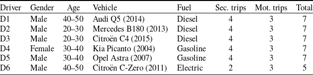

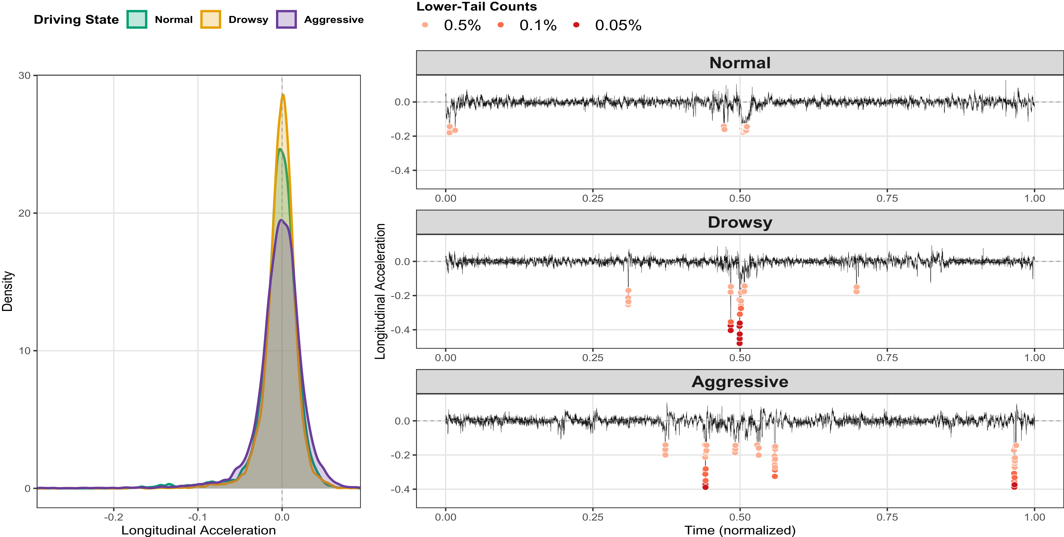
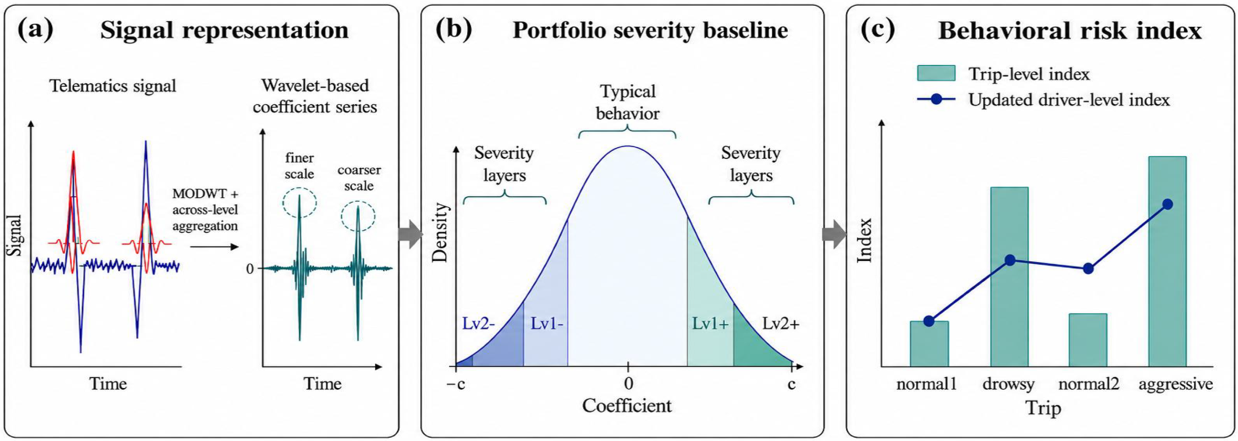
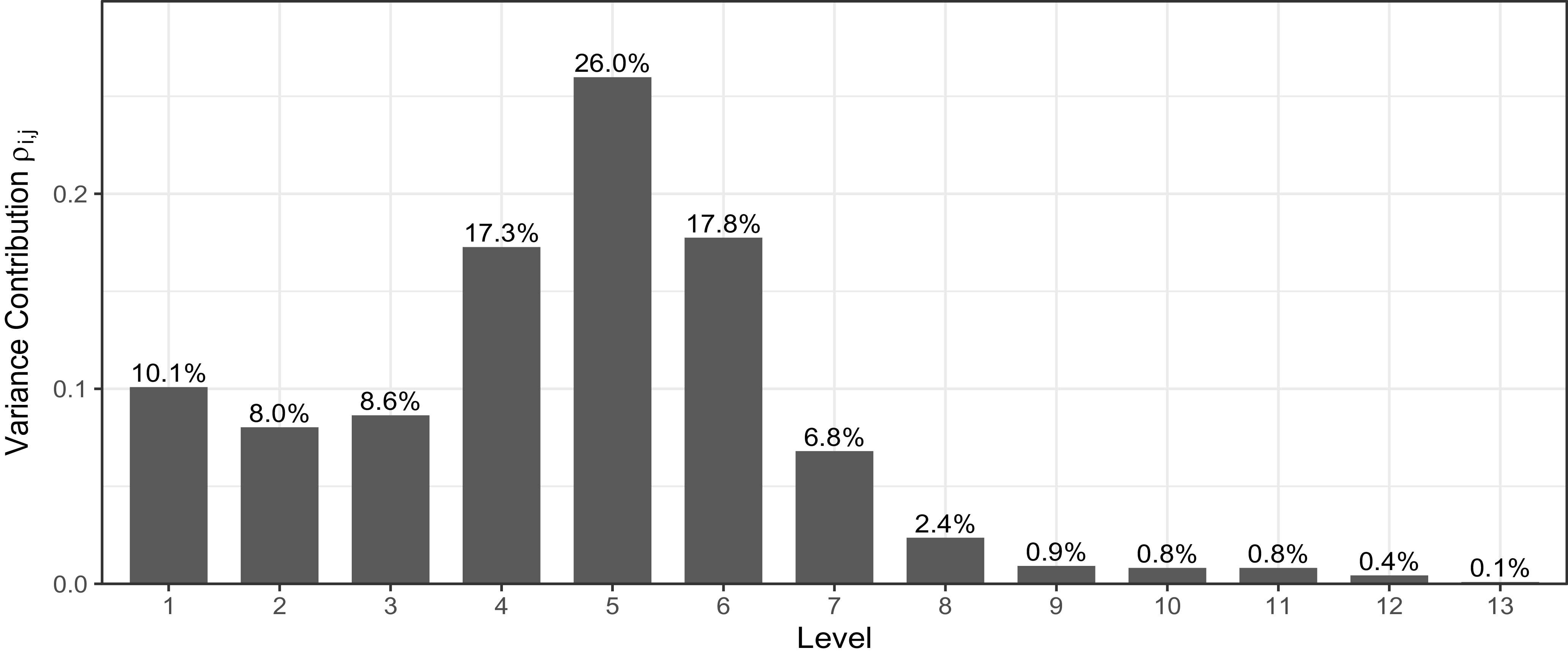
 J=6
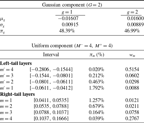
 μg
 σg
 πg
 πm
 wm
 γ⋆=0.9
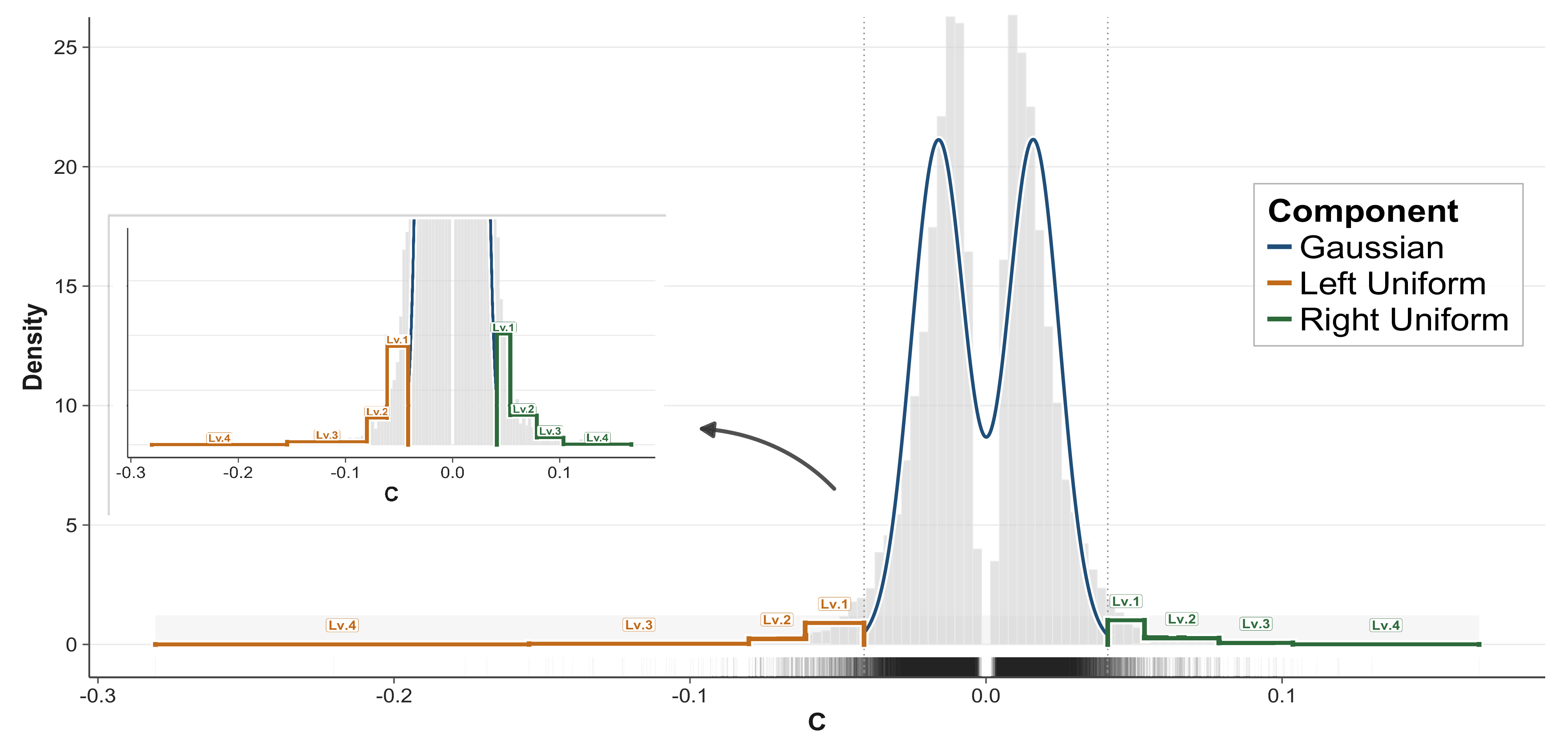
 C
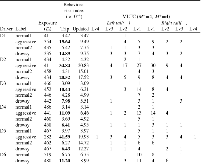
 Ei:=|Ti|
 ∼
 ∼
 (M−=4,M+=4)
 γ⋆=0.9
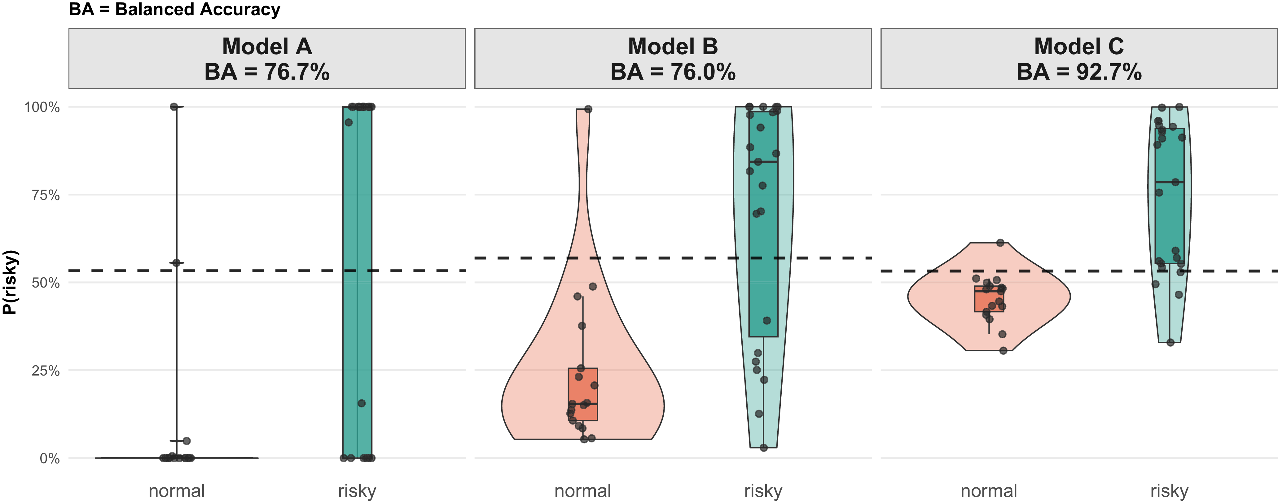
 P(risky)
 γ⋆=0.9
 γ
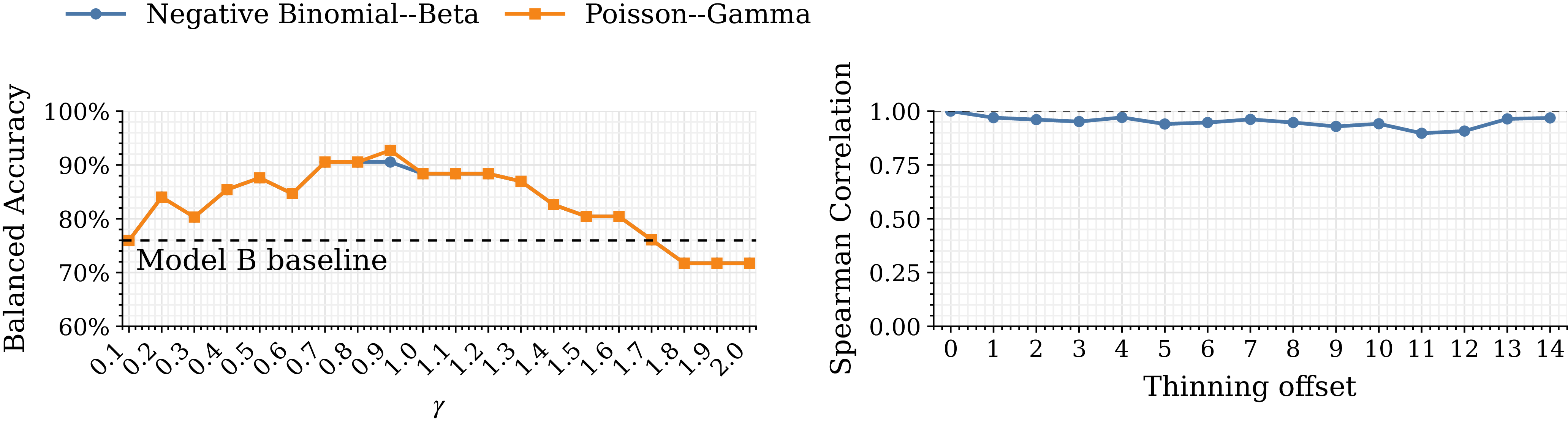
 γ∈{0.1,…,2.0}
 =76.0%
 Lglobal=15


 Open access

