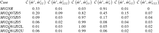
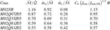
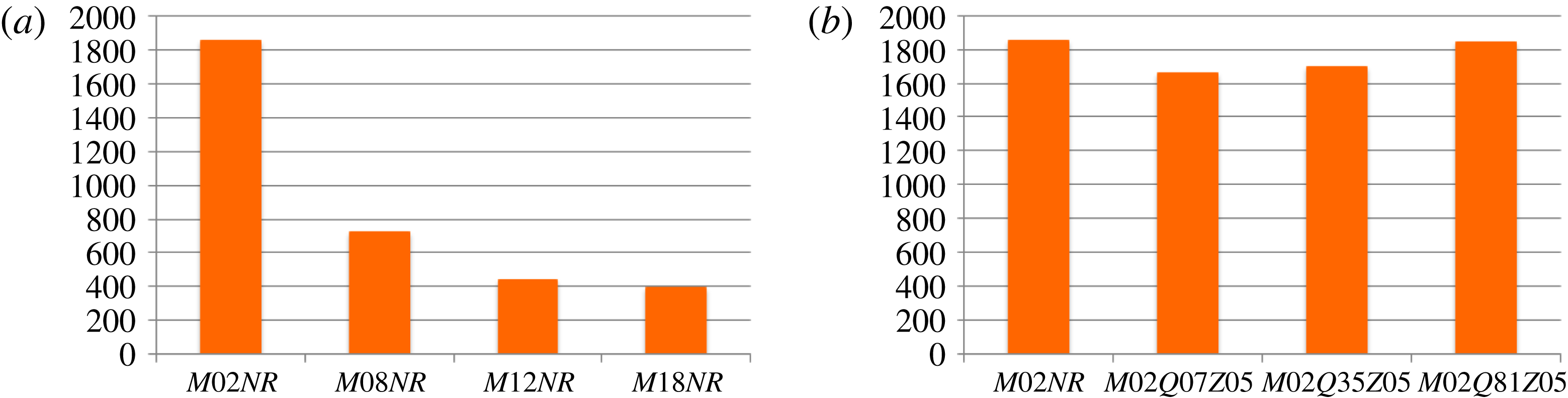
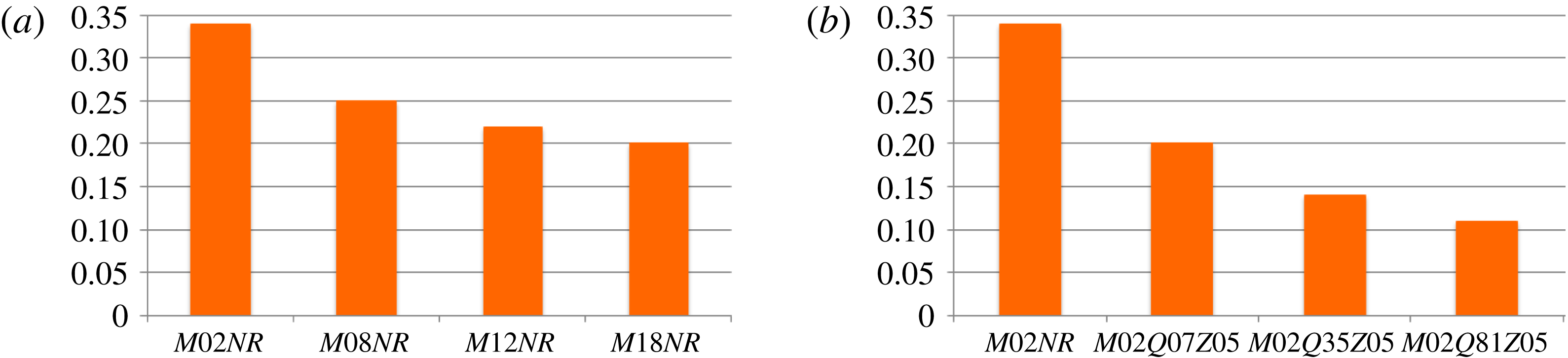
1 Introduction
The study of the turbulent flows which are surrounded by laminar regions of fluid motions is of great importance in many engineering applications. Examples of such flows are free shear flows (jets, plumes, wakes, mixing layers), turbulent boundary layers, many of the atmospheric and oceanic flows and gravity currents. The free shear flows are seen in many engineering and environmental applications which makes the fundamental study of this type of turbulent flows both practically demanding and theoretically intriguing. Furthermore, in most practical combustion applications, such as aircraft or car engines, the region of the flow in which combustion takes place is turbulent. In non-premixed reacting systems, mixing must bring reactants into the reaction zone fast enough for combustion to occur. The initial stage of this process is done by entrainment. Therefore, it is important to study the entrainment in turbulent reacting flows.
An important feature of the turbulent flows surrounded by irrotational regions is a sharp and highly convoluted interface that separates the fully turbulent and laminar regions (Corrsin & Kistler Reference Corrsin and Kistler1955). This interface is referred to as the turbulent/non-turbulent interface (TNTI) and is the surface on which entrainment occurs. In the present study, the term entrainment process is used to describe all the mechanisms that are responsible for the transfer of mass across the boundaries of the turbulent flow. This process, which is responsible for growth of the turbulent region into the irrotational region, is associated with two mechanisms: nibbling, which is considered to be carried out by small-scale eddies, and engulfment, which is mostly due to large-scale structures (Mathew & Basu Reference Mathew and Basu2002; Westerweel et al. Reference Westerweel, Fukushima, Pedersen and Hunt2005). The entrainment due to nibbling is related to the outward spreading of small vortices under the turbulent boundaries (Westerweel et al. Reference Westerweel, Fukushima, Pedersen and Hunt2005). On the other hand, the entrainment due to engulfment is done by digestion of pockets of the ambient flow into the turbulent region (Mathew & Basu Reference Mathew and Basu2002). Engulfment was generally considered to be the principle mechanism of entrainment for all turbulent free shear flows (Brown & Roshko Reference Brown and Roshko1974; Dimotakis & Brown Reference Dimotakis and Brown1976; Dahm & Dimotakis Reference Dahm and Dimotakis1987; Ferré et al. Reference Ferré, Mumford, Savill and Giralt1990; Mungal, Karasso & Lozano Reference Mungal, Karasso and Lozano1991; Dimotakis Reference Dimotakis2000; Bisset, Hunt & Rogers Reference Bisset, Hunt and Rogers2002). However, recent experimental and numerical works on non-reacting turbulent jets and mixing layers have shown that engulfing motions do not dominate the entrainment, as they only contribute to a small percentage of the total entrained mass flow rate (Westerweel et al. Reference Westerweel, Fukushima, Pedersen and Hunt2005, Reference Westerweel, Fukushima, Pedersen and Hunt2009; Hunt et al. Reference Hunt, Eames, da Silva and Westerweel2011; Taveira et al. Reference Taveira, Diogo, Lopes and da Silva2013; da Silva, Taveira & Borrell Reference da Silva, Taveira and Borrell2014b ; Jahanbakhshi & Madnia Reference Jahanbakhshi and Madnia2016).
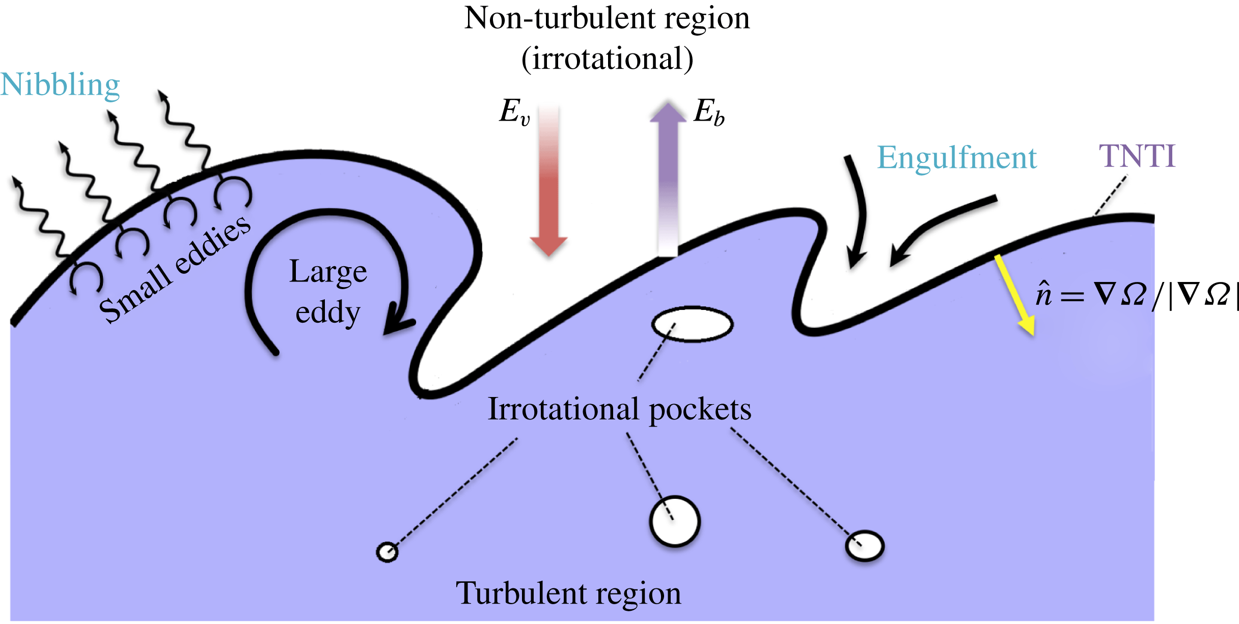
Figure 1 shows a schematic of the entrainment process. In order to study the entrainment of non-turbulent flow into the turbulent region, one must first find a quantifiable distinction between these two regions of flow. One of the physically quantitative differences between the laminar and turbulent regions is that turbulent flows are rotational, whereas, laminar ones are practically irrotational (Corrsin & Kistler Reference Corrsin and Kistler1955). Mathematically, the tendency of a fluid element to rotate is determined by the vorticity pseudo-vector. Therefore, the most distinctive feature between the flow regions separated by the TNTI consists of the strong contrast between the total absence of vorticity in the irrotational zone and the high vorticity content of the turbulent zone (Tsinober Reference Tsinober2000). Thus, the interface between the turbulent and the non-turbulent regions is found by a vorticity magnitude in the temporal mixing layers of the current work. It should be pointed out that in spatially developing shear flows, in which the laminar, the transitional, and the fully turbulent region exist at the same time in different locations in the flow, vorticity magnitude by itself cannot be used to detect the turbulent region. For example in a spatially evolving boundary layer, Lee & Zaki (Reference Lee and Zaki2016) suggested identifying the fully turbulent region and the turbulent spots in the transitional region using the vorticity magnitude excluding the spanwise component since it is large even in the laminar region.
In figure 1, nibbling is considered as the vorticity transport across the TNTI, which occurs on the entire TNTI isosurface. The mass flow rate associated with nibbling is computed as the surface area of the TNTI multiplied by the mass flux across it. The mass flux across the TNTI is proportional to the velocity of the fluid element relative to the TNTI referred to as local entrainment velocity. Therefore, the nibbling mechanism is usually studied by finding the local entrainment velocity (Holzner & Lüthi Reference Holzner and Lüthi2011; Wolf et al. Reference Wolf, Holzner, Lüthi, Krug, Kinzelbach and Tsinober2013; Chauhan et al. Reference Chauhan, Philip, de Silva, Hutchins and Marusic2014; Krug et al. Reference Krug, Holzner, Lüthi, Wolf, Kinzelbach and Tsinober2015; Philip et al. Reference Philip, Bermejo-Moreno, Chung and Marusic2015; Jahanbakhshi & Madnia Reference Jahanbakhshi and Madnia2016; Mistry et al. Reference Mistry, Philip, Dawson and Marusic2016; Holzner & van Reeuwijk Reference Holzner and van Reeuwijk2017; Krug et al. Reference Krug, Chung, Philip and Marusic2017; van Reeuwijk, Krug & Holzner Reference van Reeuwijk, Krug and Holzner2018). In these works, it is shown that the local entrainment on the TNTI is dependent on the local curvatures and local dilatation of the TNTI isosurface as well as local baroclinic torque in buoyant or compressible flows. In the past decade a number of other works have been devoted to the study of transport mechanisms across the TNTI in different types of turbulent flows which are related to nibbling (Westerweel et al. Reference Westerweel, Fukushima, Pedersen and Hunt2005; Hunt, Eames & Westerweel Reference Hunt, Eames and Westerweel2006; Holzner et al. Reference Holzner, Liberzon, Nikitin, Kinzelbach and Tsinober2007; da Silva & Pereira Reference da Silva and Pereira2008; Anand, Boersma & Agrawal Reference Anand, Boersma and Agrawal2009; Westerweel et al. Reference Westerweel, Fukushima, Pedersen and Hunt2009; Hunt et al. Reference Hunt, Eames, da Silva and Westerweel2011; Gampert et al. Reference Gampert, Narayanaswamy, Schaefer and Peters2013; Khashehchi et al. Reference Khashehchi, Ooi, Soria and Marusic2013; Taveira & da Silva Reference Taveira and da Silva2013; Jahanbakhshi, Vaghefi & Madnia Reference Jahanbakhshi, Vaghefi and Madnia2015; Vaghefi & Madnia Reference Vaghefi and Madnia2015). All of these works are specific to non-reacting turbulence. Investigating the local statistics of the turbulence in the regions near the TNTI helps to better understand the entrainment process. In order to do this, Bisset et al. (Reference Bisset, Hunt and Rogers2002) for the first time proposed the use of conditional statistics based on the distance from the TNTI. A detailed review of this type of analysis of entrainment can be found in the previous work by da Silva et al. (Reference da Silva, Hunt, Eames and Westerweel2014a ).
Schematic of the entrainment process. Included are:
 $\hat{n}$
the unit vector normal to the TNTI,
 $E_{b}$
the boundary entrainment velocity,
 $E_{v}$
the induced velocity, pockets of irrotational flow inside turbulent region and main physical mechanisms contributing to entrainment, nibbling and engulfment.
 $\unicode[STIX]{x1D6FA}=\unicode[STIX]{x1D714}_{i}\unicode[STIX]{x1D714}_{i}$
is the enstrophy.

In figure 1, engulfment is considered as the drawing of the pockets of outside irrotational fluid into the turbulent region (Mathew & Basu Reference Mathew and Basu2002; Taveira et al. Reference Taveira, Diogo, Lopes and da Silva2013; da Silva et al. Reference da Silva, Taveira and Borrell2014b ). Most of these pockets eventually break down inside the turbulent region and become turbulent. However, some of them might join together and create larger pockets or exit the turbulent region. In order to study the engulfment, all of the irrotational pockets, which are completely embedded inside the turbulent region, need to be found and examined separately. These pockets can either be created inside the turbulent region or be drawn into the shear layer from outside. In an Eulerian approach it is difficult to determine the origin of the individual irrotational pockets. Therefore, in the previous works different methods are used to overcome this difficulty. In some cases the engulfment is studied by comparing the results with the results of a homogeneous isotropic turbulence, in which all of the irrotational pockets are generated inside the turbulent region (da Silva et al. Reference da Silva, Taveira and Borrell2014b ; Jahanbakhshi & Madnia Reference Jahanbakhshi and Madnia2016); a few other works estimated the average mass flow rate of the irrotational pockets in the streamwise direction and associated that mass with the engulfment (Westerweel et al. Reference Westerweel, Fukushima, Pedersen and Hunt2005, Reference Westerweel, Fukushima, Pedersen and Hunt2009); others draw a conclusion based on the study of the individual large-scale coherent structures or the conditional statistics of the mean and fluctuating flow variables near the TNTI (Bisset et al. Reference Bisset, Hunt and Rogers2002; Philip & Marusic Reference Philip and Marusic2012; Hickey, Hussain & Wu Reference Hickey, Hussain and Wu2013); and finally there has also been a Lagrangian analysis of the engulfment (Taveira et al. Reference Taveira, Diogo, Lopes and da Silva2013). In these works, it is reported that the contribution of the engulfment to total entrainment is small in non-reacting turbulent jets and mixing layers, whereas the entrainment in a non-reacting wakes is primarily driven by the engulfment. The entrainment process can also be viewed by a multi-scale approach. Philip et al. (Reference Philip, Meneveau, de Silva and Marusic2014) and Mistry et al. (Reference Mistry, Philip, Dawson and Marusic2016) have studied the entrainment process in a turbulent boundary layer and an axisymmetric jet by this approach respectively. In their work, the fluxes of various transport mechanisms across the TNTI are related to a hierarchy of length scales by spatial filtering of the data as used commonly in large eddy simulation. These fluxes are divided into two categories: the flux at small scales, which is associated with nibbling, and the flux at large scales to be associated with engulfment. Using this multi-scale perspective, they reported that the qualitative trends from the measurement results provide evidence that large-scale transport due to the energy-containing eddies determines the overall rate of entrainment, while viscous effects at the smallest scales provide the physical mechanism ultimately responsible for entrainment.
Most of the previous works, which have studied the entrainment process in reacting turbulent shear flows, have focused on the effect of heat release on the overall growth rate of the shear layer (Hermanson & Dimotakis Reference Hermanson and Dimotakis1989; McMurtry, Riley & Metcalfe Reference McMurtry, Riley and Metcalfe1989; Sekar & Mukunda Reference Sekar and Mukunda1991; Miller, Madnia & Givi Reference Miller, Madnia and Givi1995; Livescu, Jaberi & Madnia Reference Livescu, Jaberi and Madnia2002; Pantano, Sarkar & Williams Reference Pantano, Sarkar and Williams2003; Mahle et al. Reference Mahle, Foysi, Sarkar and Friedrich2007; Mathew, Mahle & Friedrich Reference Mathew, Mahle and Friedrich2008; O’Brien et al. Reference O’Brien, Urzay, Ihme, Moin and Saghafian2014). While all of these works have reported a reduction in growth rate due to the effects of heat release, none have quantified the mass that enters the shear layer. In several previous experimental works on reacting and non-reacting spatial mixing layers (Brown Reference Brown1975; Dimotakis Reference Dimotakis1986; Hermanson & Dimotakis Reference Hermanson and Dimotakis1989) and spatial jets (Ricou & Spalding Reference Ricou and Spalding1961; Becker & Yamazaki Reference Becker and Yamazaki1978; Muniz & Mungal Reference Muniz and Mungal2001), in which the two mixing streams have a density difference, it is estimated that the entrainment at different locations along the axis of a free shear layer is proportional to the root of density ratio of two streams. In another work, Dahm (Reference Dahm2005) has proposed that the effects of heat release on the growth rate of exothermic reacting mixing layers can be characterized by finding an extended density ratio, and using this density ratio in the equations obtained for the non-reacting mixing layers.
To the best of our knowledge, the study of the entrainment near the TNTI in compressible reacting turbulent flows has not been done previously. In our previous work, the effect of compressibility on the entrainment in non-reacting mixing layers is studied by examining several cases with convective Mach number ranging from 0.2 to 1.8 (Jahanbakhshi & Madnia Reference Jahanbakhshi and Madnia2016). In this work, it is shown that the primary effect of compressibility on the entrainment is a decrease of surface area of the TNTI while the local entrainment velocity reduces moderately. Furthermore for the range of compressibility studied in Jahanbakhshi & Madnia (Reference Jahanbakhshi and Madnia2016), it is observed that the contribution of the baroclinic term in the enstrophy transport equation to the mean local entrainment velocity remains small (approximately 8 % for the case with the highest level of compressibility). The main objectives of the present work are to study the effect of heat release and flame location on the mechanisms of entrainment, i.e. nibbling and engulfment, and to determine the similarities and the differences between the effects of compressibility and heat release on them.
This paper is organized as follows. In § 2 a summary of the direct numerical simulation (DNS) results for the compressible reacting mixing layer is provided, and the numerical results are compared with published experimental and numerical studies to validate the DNS data. In § 3, the method used to detect the turbulent/non-turbulent interface, the interaction between the flame and the TNTI and some of the characteristics of the TNTI are studied. In § 4, the mechanisms contributing to the entrainment, i.e. nibbling and engulfment, are investigated, and the effects of compressibility and heat release on the entrainment are compared with each other. Finally in § 5 this work ends with a summary of the findings.
2 DNS of compressible reacting mixing layers
A brief description of the DNS of the mixing layers performed for the current work is presented in this section. A more detailed representation of the DNS is provided in Jahanbakhshi (Reference Jahanbakhshi2016).
Due to high computational cost, the usage of a detailed chemistry for modelling the combustion in DNS codes is rare, and so far the vast majority of computational works in turbulent combustion have relied on reduced chemical mechanisms (Poinsot & Veynante Reference Poinsot and Veynante2005; Saghafian Reference Saghafian2014). In the present work, the combustion is mimicked by a one-step irreversible global reaction that involves fuel (
 $F$
), oxidizer (
 $O$
) and product (
 $P$
),
 $$\begin{eqnarray}\unicode[STIX]{x1D708}_{F}F+\unicode[STIX]{x1D708}_{O}O\longrightarrow \unicode[STIX]{x1D708}_{P}P,\end{eqnarray}$$
where
 $\unicode[STIX]{x1D708}_{\unicode[STIX]{x1D6FC}}$
is the molar stoichiometric coefficient of species
 $\unicode[STIX]{x1D6FC}$
. In addition, the molecular diffusion processes are simplified by neglecting the Soret and Dufour effects (Ern & Giovangigli Reference Ern and Giovangigli1994). Fick’s law (Kuo Reference Kuo2005) without velocity correction is used to model the diffusion velocity of species. The Schmidt number for all species is assumed to be constant. All external forces are assumed to be negligible in current simulations.
The equilibrium or fast chemistry approximation, which assumes that the time scales of the chemical reactions are much shorter than the turbulent flow time scales (Williams Reference Williams1985), is used. This approach allows the computation of the species mass fraction and the temperature from a conserved scalar, thus, significantly reducing the computational cost. Although this model is based on a low Mach number assumption, it is shown that it can be extended to high Mach number flows by using the infinitely fast assumption to only compute the species mass fractions, and then to calculate the temperature from the transport equation of an energy parameter (such as internal energy) which does not contain a source term for the reaction (Oevermann Reference Oevermann2000; Pantano-Rubino Reference Pantano-Rubino2000; Pantano et al. Reference Pantano, Sarkar and Williams2003; Mahle Reference Mahle2007). In the present work, this approach is used to model the combustion by using the mixture fraction as the conserved scalar. Mixture fraction is essentially a measure of local equivalence ratio (Bilger Reference Bilger1976; Pitsch & Peters Reference Pitsch and Peters1998; Poinsot & Veynante Reference Poinsot and Veynante2005). The kinetics of hydrogen oxidation are fast in comparison to transport processes (Faeth & Samuelsen Reference Faeth and Samuelsen1986). This makes hydrogen/air flame a good candidate for study at the fast chemistry limit.
In order to obtain the DNS data of temporally evolving mixing layers, the non-dimensional form of the conservation equations for mass, momentum, internal energy and mixture fraction are solved for compressible flow variables, i.e. density,
 $\unicode[STIX]{x1D70C}$
, velocity in the
 $x_{i}$
direction,
 $u_{i}$
, internal energy,
 $e$
, and mixture fraction,
 $Z$
,
 $$\begin{eqnarray}\displaystyle & \displaystyle \frac{\unicode[STIX]{x2202}\unicode[STIX]{x1D70C}}{\unicode[STIX]{x2202}t}+\frac{\unicode[STIX]{x2202}\left(\unicode[STIX]{x1D70C}u_{j}\right)}{\unicode[STIX]{x2202}x_{j}}=0, & \displaystyle\end{eqnarray}$$
 $$\begin{eqnarray}\displaystyle & \displaystyle \frac{\unicode[STIX]{x2202}\left(\unicode[STIX]{x1D70C}u_{i}\right)}{\unicode[STIX]{x2202}t}+\frac{\unicode[STIX]{x2202}\left(\unicode[STIX]{x1D70C}u_{j}u_{i}\right)}{\unicode[STIX]{x2202}x_{j}}=-\frac{\unicode[STIX]{x2202}p}{\unicode[STIX]{x2202}x_{i}}+\frac{1}{Re}\frac{\unicode[STIX]{x2202}\unicode[STIX]{x1D70F}_{ij}}{\unicode[STIX]{x2202}x_{j}}, & \displaystyle\end{eqnarray}$$
 $$\begin{eqnarray}\displaystyle & \displaystyle \frac{\unicode[STIX]{x2202}\left(\unicode[STIX]{x1D70C}e\right)}{\unicode[STIX]{x2202}t}+\frac{\unicode[STIX]{x2202}\left(\unicode[STIX]{x1D70C}u_{j}e\right)}{\unicode[STIX]{x2202}x_{j}}=-\frac{1}{PrRe}\frac{\unicode[STIX]{x2202}q_{j}}{\unicode[STIX]{x2202}x_{j}}+\frac{Ec}{Re}\unicode[STIX]{x1D70F}_{ij}\frac{\unicode[STIX]{x2202}u_{i}}{\unicode[STIX]{x2202}x_{j}}-pEc\frac{\unicode[STIX]{x2202}u_{j}}{\unicode[STIX]{x2202}x_{j}}, & \displaystyle\end{eqnarray}$$
 $$\begin{eqnarray}\displaystyle & \displaystyle \frac{\unicode[STIX]{x2202}\left(\unicode[STIX]{x1D70C}Z\right)}{\unicode[STIX]{x2202}t}+\frac{\unicode[STIX]{x2202}\left(\unicode[STIX]{x1D70C}u_{i}Z\right)}{\unicode[STIX]{x2202}x_{i}}=\frac{1}{Re}\frac{\unicode[STIX]{x2202}}{\unicode[STIX]{x2202}x_{i}}\left(\frac{\unicode[STIX]{x1D707}}{Sc}\frac{\unicode[STIX]{x2202}Z}{\unicode[STIX]{x2202}x_{i}}\right), & \displaystyle\end{eqnarray}$$
where
 $$\begin{eqnarray}\unicode[STIX]{x1D70F}_{ij}=\unicode[STIX]{x1D707}\left(\frac{\unicode[STIX]{x2202}u_{i}}{\unicode[STIX]{x2202}x_{j}}+\frac{\unicode[STIX]{x2202}u_{j}}{\unicode[STIX]{x2202}x_{i}}\right)-\frac{2}{3}\unicode[STIX]{x1D707}\frac{\unicode[STIX]{x2202}u_{k}}{\unicode[STIX]{x2202}x_{k}}\unicode[STIX]{x1D6FF}_{ij},\quad q_{j}=-\unicode[STIX]{x1D705}\frac{\unicode[STIX]{x2202}T}{\unicode[STIX]{x2202}x_{j}}-Pr\mathop{\sum }_{\unicode[STIX]{x1D6FC}}\frac{\unicode[STIX]{x1D707}}{Sc}h_{\unicode[STIX]{x1D6FC}}\frac{\unicode[STIX]{x2202}Y_{\unicode[STIX]{x1D6FC}}}{\unicode[STIX]{x2202}x_{j}}.\end{eqnarray}$$
In these equations Stokes’ hypothesis and Fourier’s heat conduction are assumed. Temperature,
 $T$
, and pressure,
 $p$
, are computed using non-dimensional form of the thermodynamic relation and the equation of state for an ideal gas, respectively,
 $$\begin{eqnarray}e=\int _{T_{0}}^{T}C_{p}\,\text{d}T-RT+\mathop{\sum }_{\unicode[STIX]{x1D6FC}}\unicode[STIX]{x0394}h_{f,\unicode[STIX]{x1D6FC}}^{0}Y_{\unicode[STIX]{x1D6FC}},\quad p=\frac{1}{Ec}\unicode[STIX]{x1D70C}RT.\end{eqnarray}$$
In the above equations,
 $\unicode[STIX]{x1D707}$
is the dynamic viscosity,
 $\unicode[STIX]{x1D705}$
is the thermal conductivity,
 $h_{\unicode[STIX]{x1D6FC}}$
and
 $Y_{\unicode[STIX]{x1D6FC}}$
are the enthalpy and the mass fraction of species
 $\unicode[STIX]{x1D6FC}$
respectively,
 $R=R_{0}\sum _{\unicode[STIX]{x1D6FC}}Y_{\unicode[STIX]{x1D6FC}}/{\mathcal{W}}_{\unicode[STIX]{x1D6FC}}$
is the mixture gas constant,
 $R_{0}$
is the universal ideal gas constant,
 ${\mathcal{W}}_{\unicode[STIX]{x1D6FC}}$
is the molecular weight of species
 $\unicode[STIX]{x1D6FC}$
,
 $T_{0}$
is the reference temperature,
 $C_{p}$
is the mixture specific heat at constant pressure,
 $\unicode[STIX]{x0394}h_{f,\unicode[STIX]{x1D6FC}}^{0}$
is the enthalpy of formation of species
 $\unicode[STIX]{x1D6FC}$
at temperature
 $T_{0}$
and the non-dimensional parameters are the Reynolds number,
 $Re$
, the Prandtl number,
 $Pr$
, the Schmidt number,
 $Sc$
, and the Eckert number,
 $Ec$
.
The infinitely fast approximation for reaction implies that the mass fraction of species are piecewise-linear functions of the mixture fraction (Williams Reference Williams1985),
 $$\begin{eqnarray}\displaystyle & \displaystyle Y_{F}\left(Z\right)=\left\{\begin{array}{@{}ll@{}}Y_{F}^{0}\left(Z-Z_{st}\right)/\left(1-Z_{st}\right), & \text{if}~Z\geqslant Z_{st}\\ 0, & \text{if}~Z<Z_{st}\end{array}\right., & \displaystyle\end{eqnarray}$$
 $$\begin{eqnarray}\displaystyle & \displaystyle Y_{O}\left(Z\right)=\left\{\begin{array}{@{}ll@{}}0, & \text{if}~Z\geqslant Z_{st}\\ Y_{O}^{0}\left(Z_{st}-Z\right)/Z_{st}, & \text{if}~Z<Z_{st}\end{array}\right., & \displaystyle\end{eqnarray}$$
 $$\begin{eqnarray}\displaystyle & \displaystyle Y_{P}\left(Z\right)=\frac{\unicode[STIX]{x1D708}_{P}{\mathcal{W}}_{P}Y_{F}^{0}}{\unicode[STIX]{x1D708}_{F}{\mathcal{W}}_{F}}\left(Z-\frac{Y_{F}}{Y_{F}^{0}}\right), & \displaystyle\end{eqnarray}$$
where
 $Y_{F}^{0}$
and
 $Y_{O}^{0}$
are the mass fraction of fuel and oxidizer in their corresponding streams, and
 $Z_{st}$
is the stoichiometric mixture fraction.
 $Z_{st}$
is the flame position in
 $Z$
-space and is equal to
 $$\begin{eqnarray}Z_{st}=\frac{Y_{O}^{0}}{sY_{F}^{0}+Y_{O}^{0}},\end{eqnarray}$$
where
 $s=\unicode[STIX]{x1D708}_{O}{\mathcal{W}}_{O}/\unicode[STIX]{x1D708}_{F}{\mathcal{W}}_{F}$
is the mass stoichiometric ratio. Equations (2.8)–(2.10), initially derived by Burke & Schumann (Reference Burke and Schumann1928), indicate that in our simulations,
 $Z$
is equal to 1 in the fuel stream and to 0 in the oxidizer stream. In the present work, nitrogen is used as the inert gas to dilute the mixture and the mass fraction of this species is found from
 $Y_{N_{2}}=1-\sum _{\unicode[STIX]{x1D6FC}\neq N_{2}}Y_{\unicode[STIX]{x1D6FC}}$
.
To non-dimensionalize the thermochemical parameters of the mixture the reference temperature of
 $T_{0}=298\,^{\circ }\text{K}$
and the specific heat of nitrogen at
 $T_{0}$
is used. The specific heat of the species,
 $C_{p\unicode[STIX]{x1D6FC}}$
, are assumed to vary linearly with temperature. According to the thermochemical data found in the literature (Haynes Reference Haynes2014), this assumption is valid for the range of temperature of interest in this work. The specific heat of the mixture is found using the equation
 $C_{p}=\sum _{\unicode[STIX]{x1D6FC}}C_{p\unicode[STIX]{x1D6FC}}Y_{\unicode[STIX]{x1D6FC}}$
. The dynamic viscosity,
 $\unicode[STIX]{x1D707}$
, is also taken to be a function of temperature, and Sutherland’s law (Sutherland Reference Sutherland1893) is used to calculate it at each point in the flow. The thermal conductivity is found from
 $\unicode[STIX]{x1D705}=\unicode[STIX]{x1D707}C_{p}/Pr$
by assuming Prandtl number is constant in the flow, which is a reasonable approximation for the range of temperature in our simulations (Haynes Reference Haynes2014). Finally the non-dimensional heat release parameter is defined as
 $$\begin{eqnarray}Q=\frac{q_{0}Y_{F}^{0}Z_{st}}{C_{pN_{2}}^{0}T_{0}\unicode[STIX]{x1D708}_{F}{\mathcal{W}}_{F}},\end{eqnarray}$$
where
 $q_{0}=\sum _{\unicode[STIX]{x1D6FC}}\unicode[STIX]{x1D708}_{\unicode[STIX]{x1D6FC}}{\mathcal{W}}_{\unicode[STIX]{x1D6FC}}\unicode[STIX]{x0394}h_{f,\unicode[STIX]{x1D6FC}}^{0}$
is the enthalpy of reaction (Williams Reference Williams1985).
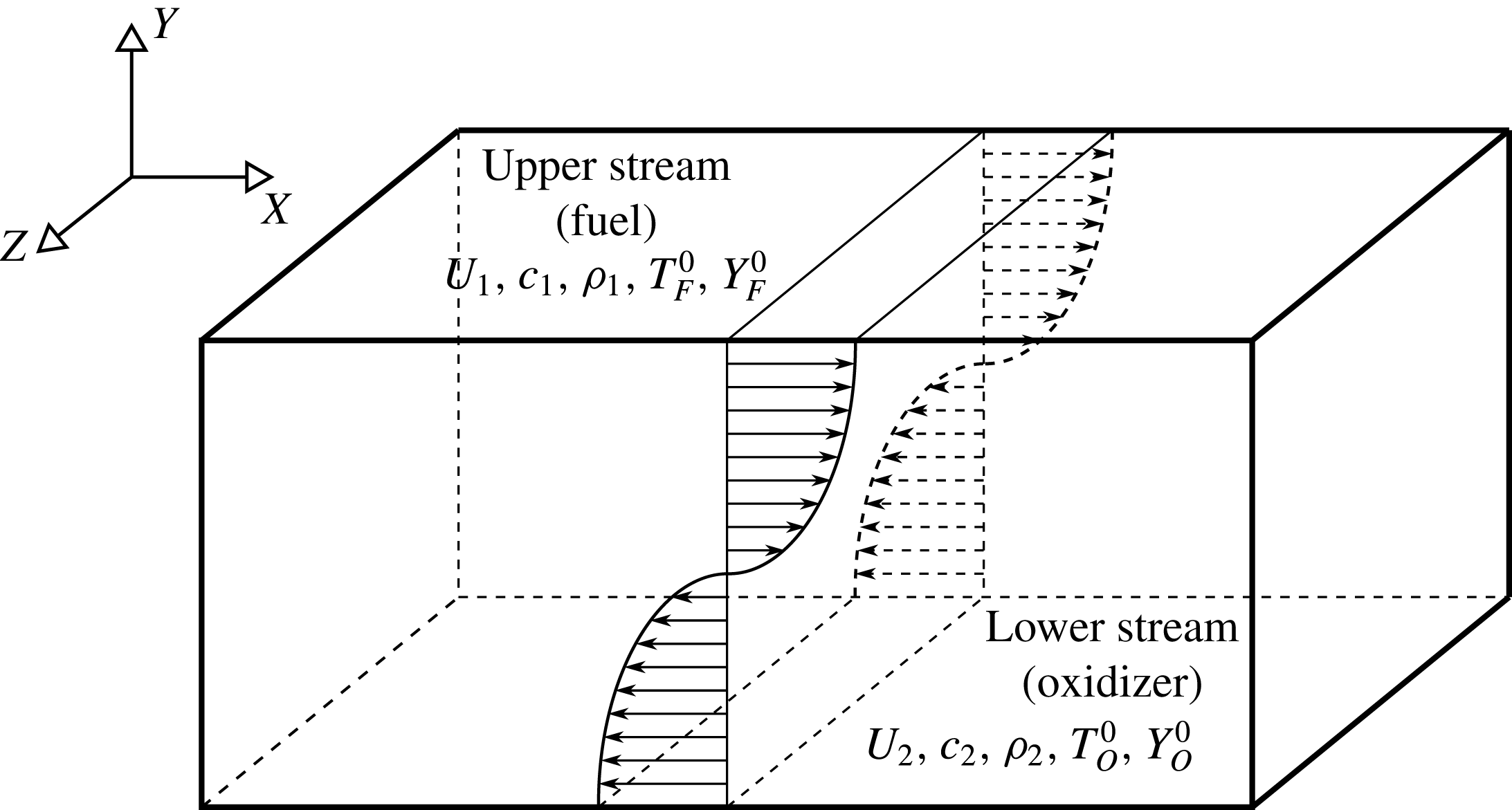
Schematic diagram of the temporally evolving shear layer. In current work
 $U_{1}=-U_{2}$
,
 $\unicode[STIX]{x1D70C}_{1}=\unicode[STIX]{x1D70C}_{2}$
, and
 $c_{1}=c_{2}$
.

Figure 2 is a sketch of the flow configuration considered in the present work. In this figure
 $x$
and
 $z$
represent homogeneous streamwise and spanwise directions respectively, and
 $y$
denotes the transverse direction. Velocity in upper stream is
 $U_{1}$
, i.e. the reference velocity, and the lower stream has a velocity
 $U_{2}=-U_{1}$
. The convective Mach number is defined as
 $M_{c}=\unicode[STIX]{x0394}U/(c_{1}+c_{2})$
, where
 $\unicode[STIX]{x0394}U=U_{1}-U_{2}$
is the velocity difference and
 $c_{1}$
and
 $c_{2}$
are the speeds of sound of each stream (Bogdanoff Reference Bogdanoff1983). The computational domain in the streamwise (
 $x$
), transverse (
 $y$
) and spanwise (
 $z$
) directions with lengths
 $L_{x}\times L_{y}\times L_{z}$
, is discretized uniformly with the number of grid points equal to
 $N_{x}\times N_{y}\times N_{z}$
. Table 1 shows the domain length and number of grids for different cases. Simulations are conducted with a parallel implementation of the two-four finite difference method of Gottlieb–Turkel scheme (Gottlieb & Turkel Reference Gottlieb and Turkel1976). Boundary conditions are periodic in homogeneous directions (
 $x$
and
 $z$
), and characteristic slip walls in the transverse direction (Thompson Reference Thompson1990; Poinsot & Veynante Reference Poinsot and Veynante2005). The initial momentum thickness,
 $\unicode[STIX]{x1D6FF}_{\unicode[STIX]{x1D703}_{0}}$
, which is the reference length scale in our simulations, is equal to unity for all the cases. The mean flow in streamwise direction is initialized with hyperbolic tangent profile and the mean transverse and spanwise velocities are zero. The initial temperature is obtained from the Busemann–Crocco relationship (Ragab & Wu Reference Ragab and Wu1989) for the non-reacting case, and from the Burke–Schumann relation (Williams Reference Williams1985) for the reacting cases. The pressure field is initially uniform, and the initial density is calculated from the equation of state for an ideal gas, equation (2.7).
It is previously reported that changing the initial density ratio of the lower and upper streams in a turbulent mixing layer will affect the entrainment process (Brown & Roshko Reference Brown and Roshko1974; Dimotakis Reference Dimotakis1991; Soteriou & Ghoniem Reference Soteriou and Ghoniem1995; Pantano & Sarkar Reference Pantano and Sarkar2002; Dahm Reference Dahm2005). Since the objective of the present work is to study the effects of heat release and flame location on the entrainment, the density of lower stream is set to be equal to the density of upper stream for all the cases. This is achieved by setting the temperature ratio of
 $T_{F}^{0}/T_{O}^{0}=R_{O}/R_{F}$
for the upper and lower streams, where
 $T_{F}^{0}$
and
 $T_{O}^{0}$
are the initial temperatures and
 $R_{F}$
and
 $R_{O}$
are the gas constants in fuel and oxidizer streams respectively. The mixture fraction is initialized with a hyperbolic tangent profile. The initial mass fractions of the oxidizer and fuel in their corresponding streams are found by using (2.11) and (2.12) and the prescribed level of heat release and stoichiometric mixture fraction for each case. To initiate turbulence, three-dimensional velocity perturbations obtained by digital filter method (Klein, Sadiki & Janicka Reference Klein, Sadiki and Janicka2003) are imposed on the mean velocities. This method generates fluctuations based on prescribed length scales and a Reynolds stress tensor satisfying a locally given autocorrelation function (Vaghefi Reference Vaghefi2014).
Simulation and turbulence parameters for the cases of the present study.
 $M_{c}$
is the convective Mach number,
 $Q$
is the non-dimensional heat release parameter,
 $Z_{st}$
is the stoichiometric mixture fraction,
 $L_{i}$
and
 $N_{i}$
are the length of the domain and the number of the grid points in
 $i$
-direction respectively,
 $\unicode[STIX]{x1D6FF}_{\unicode[STIX]{x1D703}_{0}}$
is the initial momentum thickness,
 $M_{t}$
is the turbulent Mach number,
 $Re_{\unicode[STIX]{x1D706},f}$
and
 $Re_{\unicode[STIX]{x1D714},f}$
are the Taylor and vorticity thickness Reynolds numbers at the end of the self-similar state respectively,
 $\unicode[STIX]{x1D702}_{min}/\unicode[STIX]{x0394}x$
is the minimum value of Kolmogorov length scale normalized by the grid size. N/A indicates ‘not applicable’.

Table 1 summarizes the simulation and turbulence parameters for all the cases of the present study. In this table,
 $M02NR$
is the non-reacting case. For this case (2.2) to (2.7) are solved with
 $e$
corresponding to sensible energy, i.e.
 $e=\int _{T_{0}}^{T}C_{p}\,\text{d}T-RT$
and
 $q_{j}=-\unicode[STIX]{x1D705}\unicode[STIX]{x2202}T/\unicode[STIX]{x2202}x_{j}$
. In the present work, comparison between the cases with the same
 $M_{c}$
and
 $Z_{st}$
and different
 $Q$
highlights the effects of heat release on the flow, and comparison between the cases with the same
 $Q$
and
 $M_{c}$
and different
 $Z_{st}$
shows the effects of flame location relative to TNTI on the flow. In order to have the Taylor Reynolds number for all the cases to be of the same order, different numerical Reynolds numbers, i.e. the Reynolds numbers defined based on the reference values, are used in our simulations for different cases. It is discussed by Dimotakis (Dimotakis Reference Dimotakis2005) that for
 $Re_{\unicode[STIX]{x1D706}}>100$
various flow phenomena are a weak function of the Reynolds number. This assertion is also verified for the scaling of the TNTI in turbulent planar jets and shear free turbulence with Reynolds number ranging from
 $142\leqslant Re_{\unicode[STIX]{x1D706}}\leqslant 300$
presented by da Silva in a recent conference (da Silva & Silva Reference da Silva and Silva2016). Case
 $M02NR$
represents a flow with low level of compressibility and is an approximation to an incompressible non-reacting turbulent mixing layer. The DNS simulations carried out for the present work also include cases with different convective Mach numbers, i.e.
 $0.2\leqslant M_{c}\leqslant 1.8$
. In this paper only the results of the cases with
 $M_{c}=0.2$
are reported. The results corresponding to the reacting and non-reacting cases with
 $M_{c}>0.2$
can be found in the dissertation done in our group (Jahanbakhshi Reference Jahanbakhshi2016).
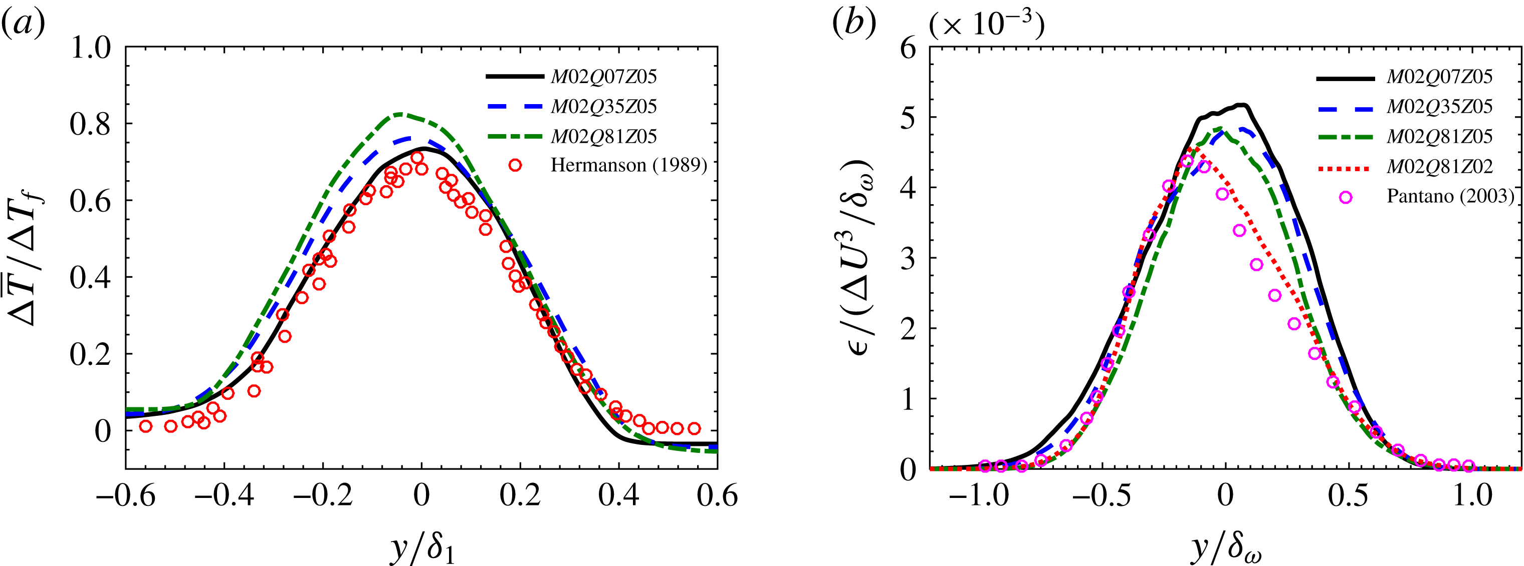
(a) Mean temperature rise profiles for the reacting cases with
 $Z_{st}=0.5$
, and (b) turbulent dissipation variation across the mixing layer for all the reacting cases.
 $\unicode[STIX]{x1D6FF}_{1}$
is the 1 % thickness based on the mean temperature profile,
 $\unicode[STIX]{x0394}\overline{T}=\overline{T}-(T_{O}^{0}+T_{F}^{0})/2$
,
 $\unicode[STIX]{x0394}T_{f}=T_{ad}-(T_{O}^{0}+T_{F}^{0})/2$
,
 $T_{ad}$
is the adiabatic flame temperature,
 $T_{F}^{0}$
and
 $T_{O}^{0}$
are the temperatures of fuel and oxidizer streams respectively,
 $\unicode[STIX]{x1D6FF}_{\unicode[STIX]{x1D714}}$
is the vorticity thickness and
 $\unicode[STIX]{x0394}U$
is the velocity difference of the two streams. The bar symbol represents averaging on the homogeneous planes.

A comprehensive validation of the DNS was performed. For all the cases, it is observed that after a transitional period, flow reaches a universal self-similar state (Redford, Castro & Coleman Reference Redford, Castro and Coleman2012) in which the mixing layer growth rate approaches a constant value, and the turbulent statistics show the self-similarity (Rogers & Moser Reference Rogers and Moser1994). In order to perform a meaningful comparison between different cases, all of the statistics are averaged over time during the self-similar state. Figure 3 shows a sample of the validation study for the current DNS data. Figure 3(
 $a$
) compares the mean temperature rise profiles of current reacting cases with the experimental results of Hermanson & Dimotakis (Reference Hermanson and Dimotakis1989) corresponding to spatially developing mixing layers with low heat release levels, i.e.
 $0.3<Q<0.8$
. This figure shows there is good agreement between the experimental results and the current DNS case with
 $Q=0.7$
. Figure 3(b) shows comparison of the normalized turbulent dissipation with a previous numerical work done by Pantano et al. (Reference Pantano, Sarkar and Williams2003) corresponding to a temporally evolving mixing layer which has a heat release level and stoichiometric mixture fraction close to case
 $M02Q81Z02$
. It can be seen that the shape of the profiles and the peak values are generally in good agreement. Three supplementary movies, which are generated from the simulation data corresponding to case
 $M02Q81Z05$
, are available at https://doi.org/10.1017/jfm.2018.122. A more detailed validation of the DNS cases of the present work can be found in Jahanbakhshi (Reference Jahanbakhshi2016) and Vaghefi (Reference Vaghefi2014).
The averaging of the statistics in the present work is performed in two stages: computing the average in space followed by averaging in time during the self-similar state. For an arbitrary quantity
 ${\mathcal{X}}$
three different averages are defined here; the average on homogeneous planes, denoted as
 $\overline{{\mathcal{X}}}$
, is the ensemble average of
 ${\mathcal{X}}$
on the plane
 $y=\text{const.}$
, the average on the TNTI, denoted as
 $\langle {\mathcal{X}}\rangle$
, is the ensemble average on a vorticity magnitude isosurface that defines the TNTI, and finally the symbol
 $\langle {\mathcal{X}}\rangle _{I}$
is used to denote the ensemble average of
 ${\mathcal{X}}$
on the envelope of the surface
 $y_{I}=$
constant, where
 $y_{I}$
is the normal distance from the TNTI.
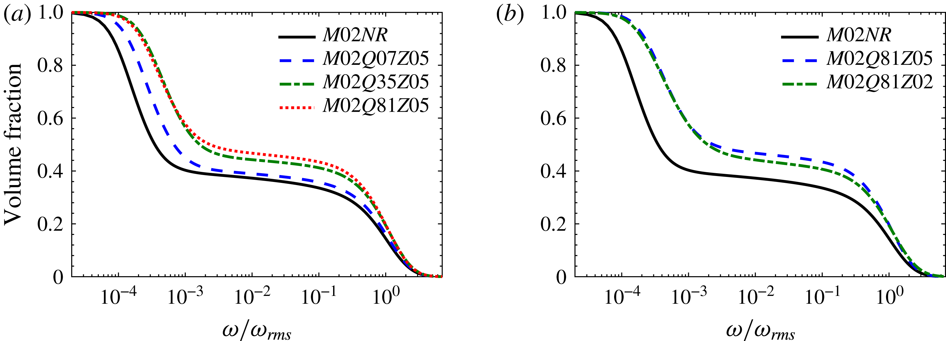
Volume fraction of the region with vorticity magnitude greater than a given threshold. (a) The effect of heat release and (b) the effect of flame location.
 $\unicode[STIX]{x1D714}_{rms}$
is the value of the root mean square of vorticity magnitude in the centre plane of the mixing layer.

3 TNTI and its interaction with the flame
The interface between turbulent and non-turbulent regions is usually detected with the vorticity magnitude (Bisset et al.
Reference Bisset, Hunt and Rogers2002; da Silva & Pereira Reference da Silva and Pereira2008; Borrell & Jiménez Reference Borrell and Jiménez2016),
 $\unicode[STIX]{x1D714}=\sqrt{\unicode[STIX]{x1D714}_{i}\unicode[STIX]{x1D714}_{i}}$
, where
 $\unicode[STIX]{x1D714}_{i}$
are vorticity components. In the present work, a certain threshold for vorticity magnitude is chosen for the turbulent region, below which flow can be considered to be irrotational. Following the same procedure as the one explained by Bisset et al. (Reference Bisset, Hunt and Rogers2002), turbulent/non-turbulent interface (TNTI) thresholds,
 $\unicode[STIX]{x1D714}_{th}$
, are found for each case.
In order to examine the effect of the TNTI thresholds on the results of this work, the dependence of the volume fraction of the turbulent region on a given vorticity magnitude is depicted in figure 4 for all the cases. As can be seen in this figure, the volume fraction decreases with vorticity magnitude monotonically; however, there is a plateau of the volume fraction for a range of
 $\unicode[STIX]{x1D714}$
for all cases. Any value of vorticity magnitude on this plateau can be used to detect the turbulent/non-turbulent interface (da Silva et al.
Reference da Silva, Taveira and Borrell2014b
). In the present study, it is observed that for the TNTI threshold chosen from this region, the results are qualitatively independent of
 $\unicode[STIX]{x1D714}_{th}$
, shown in the supplementary material available at https://doi.org/10.1017/jfm.2018.122. Similar to Taveira et al. (Reference Taveira, Diogo, Lopes and da Silva2013), the thresholds used in this work are chosen to be the inflection point on the plateau in figure 4.
In the temporal mixing layers of the current study two TNTIs are detected. The upper TNTI is the interface which separates the fuel stream from the turbulent region, and the lower TNTI corresponds to the interface between the oxidizer stream and the turbulent region. It is observed that the results of the present work for the non-reacting simulations and the reacting cases in which the flame is in the middle of the mixing layer, i.e.
 $Z_{st}=0.5$
, are similar for upper and lower TNTIs. Therefore, the reported plots and statistical values for these cases correspond to the average values of lower and upper TNTIs. For the case in which the flame is closer to the lower TNTI, i.e.
 $M02Q81Z02$
, the results are different on each of the TNTIs. Thus, the results of upper and lower TNTIs for case
 $M02Q81Z02$
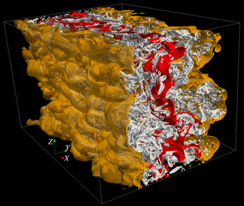
are reported separately. Figure 5 depicts a streamwise cut through the isosurfaces of discriminant of velocity gradient tensor, representing the vortical structures in the flow, for case
 $M02Q81Z05$
viewed from the lower stream. The flame and the TNTI are shown in this figure as red and translucent orange surfaces respectively. Figure 5 is a snapshot of supplementary movie 2. As can be seen, a complicated interaction exists between the flame, the TNTIs and the turbulent structures, which can change the characteristics of turbulence in reacting flows and ultimately affect the entrainment.
Streamwise cut through the mixing layer of case
 $M02Q81Z05$
viewed from the lower stream. The grey surfaces are isosurfaces of a positive value of discriminant of velocity-gradient tensor, the red surface is the flame and the orange translucent surfaces are the TNTIs.

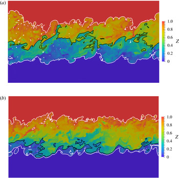
Instantaneous mixture fraction,
 $Z$
, contours in central
 $x$
–
 $y$
plane, i.e.
 $z=L_{z}/2$
, for cases (a)
 $M02Q81Z05$
and (b)
 $M02Q81Z02$
. Dark blue is the oxidizer stream and dark red is the fuel stream. The white lines correspond to the detected TNTIs and the black line corresponds to the flame.

One of the objectives of this work is to study the effect of flame location relative to TNTI on the entrainment process. The flame in the current study is the
 $Z=Z_{st}$
isosurface for each case. Figure 6 shows the
 $x$
–
 $y$
midplane corresponding to two cases with the same convective Mach number and heat release level, and different stoichiometric mixture fraction, i.e. cases
 $M02Q81Z05$
and
 $M02Q81Z02$
. This figure shows that for the case with
 $Z_{st}=0.2$
the flame is closer to the lower TNTI, and the flame/TNTI interaction can change the shape of the TNTI. Similar to the previous works on non-reacting turbulent flows (Bisset et al.
Reference Bisset, Hunt and Rogers2002; Westerweel et al.
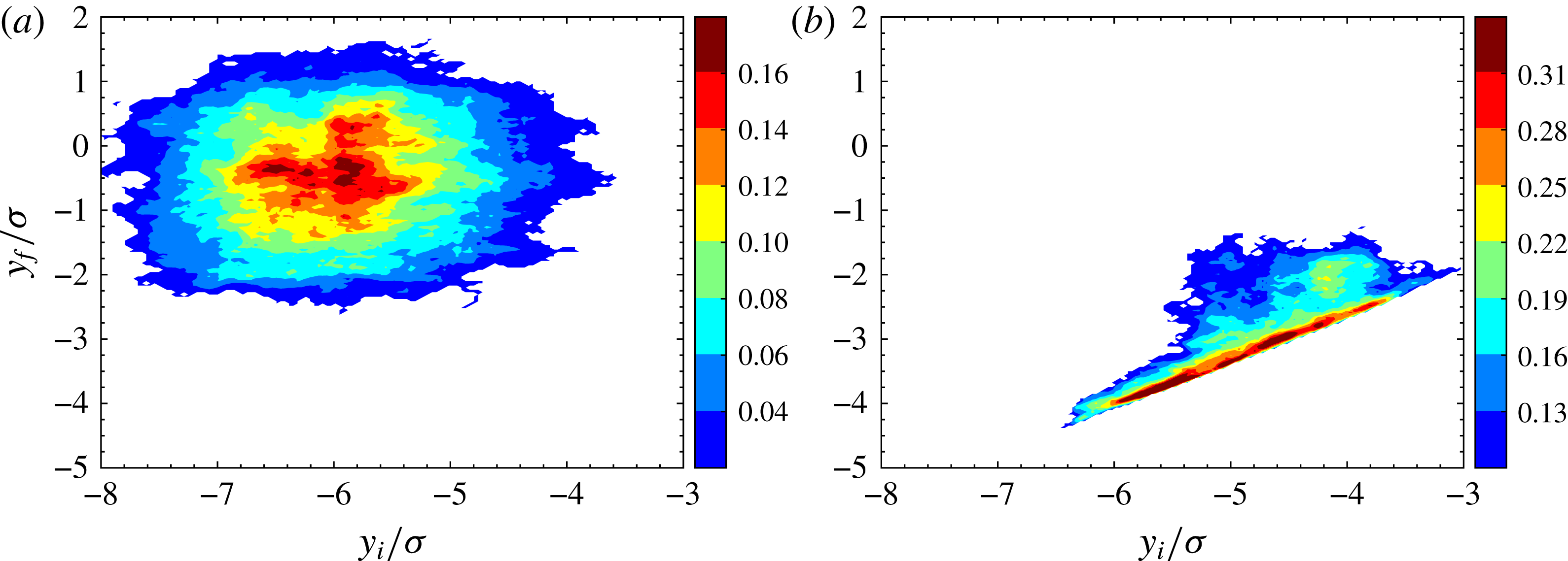
Reference Westerweel, Fukushima, Pedersen and Hunt2005; da Silva & Pereira Reference da Silva and Pereira2008; Vaghefi Reference Vaghefi2014), the probability density functions (PDFs) of the standardized vertical distance of the TNTI from the midplane are close to the Gaussian distribution for all the cases of the current study, not shown here. Similarly, the PDFs of the standardized vertical distance of the flame from the midplane resemble a Gaussian distribution. Figure 7 shows the joint probability density function (JPDF) of the locations of the flame and the lower TNTI for cases
 $M02Q81Z05$
and
 $M02Q81Z02$
. Since, the JPDF of two parameter can only be computed for equal number of grid points, in this figure, the lower envelopes of the flame and the TNTI are used. The lower envelope of a surface is defined as the outermost point of the surface in the transverse direction towards lower stream. As can be seen in figure 7, there is a clear correlation between the location of the lower TNTI and the flame for case
 $M02Q81Z02$
, whereas for case
 $M02Q81Z05$
these two parameters are practically uncorrelated.
Joint PDFs of the location of the flame envelope,
 $y_{f}$
, and the lower TNTI envelope,
 $y_{i}$
, for cases (a)
 $M02Q81Z05$
and (b)
 $M02Q81Z02$
. Each axis is normalized by its standard deviation,
 $\unicode[STIX]{x1D70E}$
.

In order to gain a better understanding of the entrainment process, it is helpful to examine the interfaces on which entrained mass flux occurs. It has been shown in incompressible turbulent flows with the presence of the mean shear, i.e. jets, wakes and boundary layers (da Silva et al. Reference da Silva, Hunt, Eames and Westerweel2014a ) and compressible mixing layers (Jahanbakhshi & Madnia Reference Jahanbakhshi and Madnia2016), that the characteristic length scale for the study of turbulent flow in proximity to the TNTI is comparable to the Taylor length scale. In this section, some of the characteristics of the TNTI in reacting compressible mixing layers are quantified. To characterize the turbulence in the proximity of the TNTI, examining the statistics conditioned on the normal distance from the TNTI has been shown to be a useful tool (da Silva et al. Reference da Silva, Hunt, Eames and Westerweel2014a ). In order to obtain the conditional statistics with respect to the normal distance from the TNTI, an interface coordinate system is defined. The origin of the new coordinate system is on the interface and its axes are tangent and normal to it respectively. More detailed description of the procedure for calculating the conditional statistics of flow variables in the interface coordinate system can be found in previous works in our group (Vaghefi Reference Vaghefi2014; Jahanbakhshi & Madnia Reference Jahanbakhshi and Madnia2016).
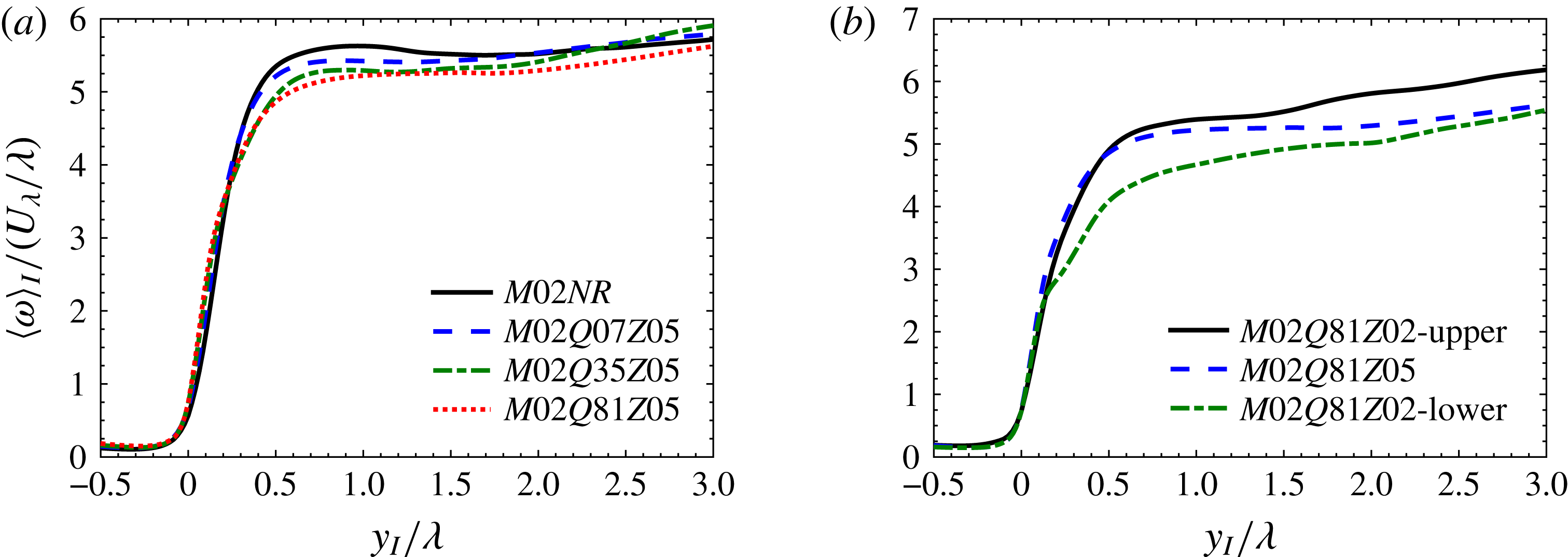
Conditional average of vorticity magnitude in the interface coordinate system. (a) The effect of heat release and (b) the effect of flame location. Profiles are normalized with the reference Taylor length scale,
 $\unicode[STIX]{x1D706}$
, and Taylor velocity scale,
 $U_{\unicode[STIX]{x1D706}}$
.

Figure 8 shows the average of vorticity magnitude,
 $\langle \unicode[STIX]{x1D714}\rangle _{I}$
, conditioned on the normal distance from the TNTI,
 $y_{I}$
, for different cases considered in the present work. In this figure, the positive and negative values of
 $y_{I}$
correspond to turbulent and irrotational regions respectively, and the distance from the TNTI is normalized with its corresponding reference Taylor length scale. It is common to use this length scale as a representation of the intermediate size of the structures in inertial sub-range of high Reynolds number turbulent flows (Pope Reference Pope2000). The conditional average of Taylor length scale is defined as
 $\langle \unicode[STIX]{x1D706}\rangle _{I}=\langle \unicode[STIX]{x1D706}_{x}+\unicode[STIX]{x1D706}_{y}+\unicode[STIX]{x1D706}_{z}\rangle _{I}/3$
, where
 $\unicode[STIX]{x1D706}_{i}$
is the Taylor length scale in the
 $i$
-direction. In order to study the characteristics of turbulence in the vicinity of the TNTI, the reference values of the Taylor length scale,
 $\unicode[STIX]{x1D706}$
, are chosen to be equal to
 $\langle \unicode[STIX]{x1D706}\rangle _{I}$
in the regions near the TNTI.
Figure 8 shows that for all cases, two distinct regions can be identified inside the turbulent region; the interface layer, in which vorticity magnitude increases with a sharp jump, and the fully turbulent region, in which the increase of vorticity becomes smoother. The mean thickness of the vorticity jump in the interface layer corresponds to the thickness of the transitional region,
 $\unicode[STIX]{x1D6FF}$
, between the irrotational and fully turbulent regions (da Silva et al.
Reference da Silva, Hunt, Eames and Westerweel2014a
). Figure 8(a) shows that the thickness of this jump is approximately equal to one Taylor length scale for the non-reacting case and reacting cases with flame located far from the TNTI. Figure 8(b) reveals that similar to case
 $M02Q81Z05$
, for the upper TNTI of case
 $M02Q81Z02$
the thickness of the interface layer is close to one Taylor length scale. However, for the lower TNTI of this case, which is much closer to the flame, the interface layer is thicker,
 $\unicode[STIX]{x1D6FF}\sim 2\unicode[STIX]{x1D706}$
. For case
 $M02Q81Z02$
in the region between the flame and the lower TNTI the vortical structures are very scarce, resulting in a weakened intensification of vorticity due to vortex stretching, shown in Jahanbakhshi (Reference Jahanbakhshi2016). Consequently, the interface layer near the lower TNTI becomes thicker than the one near the upper TNTI of this case.
Conditional average of density in interface coordinate system. (a) The effect of heat release and (b) the effect of flame location. Profiles are normalized with the reference Taylor length scale,
 $\unicode[STIX]{x1D706}$
, and reference density,
 $\unicode[STIX]{x1D70C}_{0}$
.

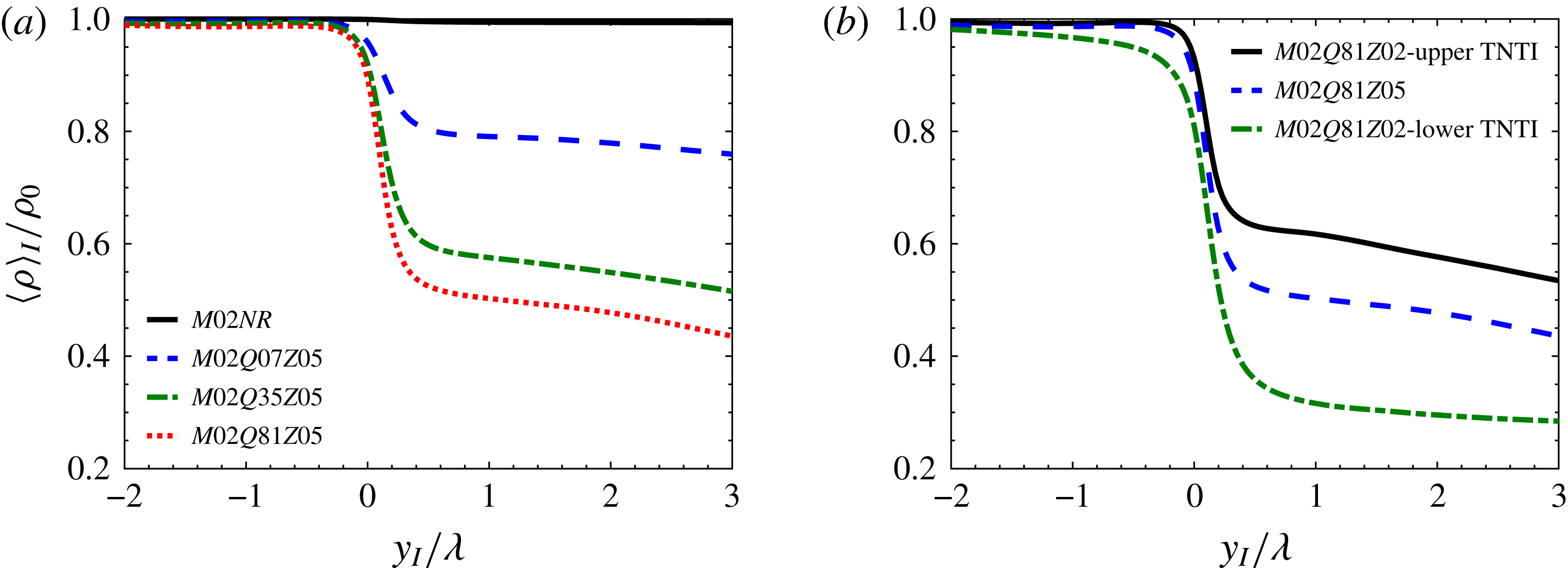
As is discussed later in § 4 one of the main effects of heat release on the entrainment is through changing the density inside the mixing layer. Figure 9 depicts the conditional average of density in interface coordinate system for all the cases. It can be seen that for case
 $M02NR$
, as expected,
 $\langle \unicode[STIX]{x1D70C}\rangle _{I}$
does not change in irrotational and turbulent regions. For the reacting cases, the mean density in irrotational flow far from the TNTI is constant; however, by moving from the irrotational region towards the turbulent region, density starts to decrease near the TNTI at
 $y_{I}\approx -0.5\unicode[STIX]{x1D706}$
for the cases with the flame far from the TNTI and at
 $y_{I}\approx -2\unicode[STIX]{x1D706}$
for the lower TNTI of case
 $M02Q81Z02$
. Near the TNTI, the mean density undergoes a sharp drop for
 $-0.2<y_{I}/\unicode[STIX]{x1D706}<0.5$
, and inside the turbulent region, i.e.
 $y_{I}/\unicode[STIX]{x1D706}>0.5$
,
 $\langle \unicode[STIX]{x1D70C}\rangle _{I}$
decreases with a smaller slope and reaches a minimum at the average location of the flame. It can be seen that as the level of heat release increases and/or the distance between the flame and the TNTI decreases, the density gradient increases near the TNTI. It is shown in § 4.2 that the large density gradients near the TNTI along with the non-barotropicity of the flow can result in vorticity generation due to mechanisms that does not exist in non-reacting incompressible flows.
In order to calculate the total entrained mass flow rate due to nibbling, the surface area of the interface on which this mass flow rate happens needs to be computed. As can be seen in figure 5 and supplementary movie 2, the entire hierarchy of the scales from the smallest to the largest structures can contribute to the increase of surface area of the TNTI. However, it is common to assume that the overall shape of the TNTI is controlled by the large-scale structures in the turbulent region (Tsinober Reference Tsinober2009; da Silva, dos Reis & Pereira Reference da Silva, dos Reis and Pereira2011; Tritton Reference Tritton2012). Furthermore in a recent work, Lee, Sung & Zaki (Reference Lee, Sung and Zaki2017) provided statistical evidence that the TNTI is locally modulated by the large-scale motions of the flow in the turbulent region. In the present work, the surface integration tool provided by ParaView is used to find the surface area of the TNTI (Ayachit Reference Ayachit2015).
The average values of surface area of the TNTI,
 ${\mathcal{A}}$
, during the self-similar state.
 ${\mathcal{A}}$
is the average of surface area of the lower and upper TNTIs for all the cases except for case
 $M02Q81Z02$
.
 $M02Q81Z02$
L and
 $M02Q81Z02$
U correspond to lower and upper TNTIs of case
 $M02Q81Z02$
.
 ${\mathcal{S}}=L_{x}\times L_{z}$
,
 $l_{x}$
and
 $l_{z}$
are the integral length scales in homogeneous directions on the midplane of the mixing layer,
 $L_{x}$
and
 $L_{z}$
are the length of the domain in homogeneous directions and
 $\unicode[STIX]{x1D6EC}=\unicode[STIX]{x1D6E4}_{t}/{\mathcal{A}}$
where
 $\unicode[STIX]{x1D6E4}_{t}$
is the volume of the turbulent region.

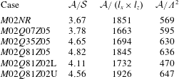
Table 2 shows the average surface area of the TNTI during the self-similar state for each case normalized by relevant length scales in the flow. It should be mentioned that the surface area changes less than 12 % in the time period, during which the averaging is performed, for all the cases. As can be seen from table 2, in the configuration studied here the surface area of the TNTI varies from 3.7 to 4.8 times the surface area of the projection of the TNTI in the transverse direction,
 ${\mathcal{S}}$
, for different cases. Therefore, one of the contributions of the large-scale structures to the entrainment is through increasing the surface area on which entrainment occurs. In temporal configurations as the mixing layer grows in time and the width of the shear layer increases, the size of the largest turbulent structures in the flow also increases. Thus, one of the parameters which can affect the surface area of the TNTI for each case is the time at which the surface area is calculated. In our simulations, the self-similarity occurs at different times for different cases. Therefore, in order to make a meaningful comparison between the surface area of the TNTI in different cases, an appropriate parameter needs to be used to normalize it. The large-scale structures inside the fully turbulent region can contribute to the change of the surface area of the TNTI. Therefore, the integral length scales in homogeneous directions,
 $l_{x}$
and
 $l_{z}$
, can be chosen to normalize the surface area of the TNTI. Furthermore, it is observed that the rate at which the volume of the turbulent region,
 $\unicode[STIX]{x1D6E4}_{t}$
, increases in time is similar to the rate at which the surface area of the TNTI increases, i.e.
 $\unicode[STIX]{x1D6E4}_{t}/{\mathcal{A}}$
is approximately constant during the self-similar state, not shown here. Thus another appropriate length scale to normalize the surface area of the TNTI is
 $\unicode[STIX]{x1D6EC}=\unicode[STIX]{x1D6E4}_{t}/{\mathcal{A}}$
. Table 2 shows that as the level of heat release increases, the surface area of the TNTI normalized by
 $l_{x}\times l_{z}$
or
 $\unicode[STIX]{x1D6EC}^{2}$
does not change significantly. Also comparing the surface area of upper and lower TNTI of case
 $M02Q81Z02$
, reveals that the TNTI closer to the flame has a smaller surface area than the one farther from the flame.
4 Local and total entrainment
Entrainment, which is responsible for growth of the turbulent region into the irrotational region and is the process by which fluid elements from the irrotational region become part of the turbulent region (Townsend Reference Townsend1976), is associated with two mechanisms; nibbling, which is considered as the vorticity transport across the TNTI, and engulfment, which is defined as the drawing of the pockets of outside irrotational fluid into the turbulent region.
The entrainment problem can be studied with a local perspective or an integral point of view (Krug et al. Reference Krug, Chung, Philip and Marusic2017). In the local perspective, the instantaneous mass flow rate into the control volume describing the turbulent region is computed by finding the velocity of the boundaries of this control volume relative to the fluid. In the integral framework, on the other hand, the entrainment is calculated by defining a bulk velocity using the change of volume inside the turbulent region. In general, there are three different velocities associated with the entrainment process (Turner Reference Turner1986), which appear in the formulation of the entrained mass flow rate. The first velocity is the rate at which irrotational fluid flows into the turbulent region across its boundaries, which is sometimes called induced velocity (Philip & Marusic Reference Philip and Marusic2012). The second velocity, referred to as the boundary entrainment velocity, is considered as the rate at which the turbulent boundaries are spreading out into the non-turbulent flow (da Silva et al. Reference da Silva, Hunt, Eames and Westerweel2014a ). The third velocity is the velocity that determines the mass flow rate across the TNTI. This velocity, which is called local entrainment velocity (Holzner & Lüthi Reference Holzner and Lüthi2011), is the relative velocity of the local fluid element and the TNTI.
In order to formulate the entrainment problem the instantaneous mass conservation in a control volume engulfing the entire volume of the turbulent region is written by using the Reynolds transport theorem, the continuity equation, and the divergence theorem respectively, as
 $$\begin{eqnarray}\dot{{\mathcal{M}}}=\frac{\text{d}}{\text{d}t}\iiint _{\unicode[STIX]{x1D6E4}_{t}}\unicode[STIX]{x1D70C}\,\text{d}{\mathcal{V}}=\iiint _{\unicode[STIX]{x1D6E4}_{t}}\frac{\unicode[STIX]{x2202}\unicode[STIX]{x1D70C}}{\unicode[STIX]{x2202}t}\,\text{d}{\mathcal{V}}-\iint _{\unicode[STIX]{x2202}\unicode[STIX]{x1D6E4}_{t}}\unicode[STIX]{x1D70C}\left(\boldsymbol{{\mathcal{U}}}^{s}\boldsymbol{\cdot }\hat{n}\right)\,\text{d}A=-\iint _{\unicode[STIX]{x2202}\unicode[STIX]{x1D6E4}_{t}}\unicode[STIX]{x1D70C}\left(\boldsymbol{V}\boldsymbol{\cdot }\hat{n}\right)\,\text{d}A,\end{eqnarray}$$
where
 $\dot{{\mathcal{M}}}$
is the change of mass inside the turbulent region,
 $\unicode[STIX]{x1D6E4}_{t}$
is the volume of the turbulent region,
 $\unicode[STIX]{x2202}\unicode[STIX]{x1D6E4}_{t}$
is the boundaries of the turbulent region,
 $\boldsymbol{{\mathcal{U}}}^{s}$
is the local velocity vector of
 $\unicode[STIX]{x2202}\unicode[STIX]{x1D6E4}_{t}$
,
 $\hat{n}$
is the inward-pointing unit vector normal to
 $\unicode[STIX]{x2202}\unicode[STIX]{x1D6E4}_{t}$
,
 $\boldsymbol{V}=\boldsymbol{{\mathcal{U}}}^{s}-\boldsymbol{{\mathcal{U}}}$
is the local velocity of
 $\unicode[STIX]{x2202}\unicode[STIX]{x1D6E4}_{t}$
relative to the fluid element and
 $\boldsymbol{{\mathcal{U}}}$
is the local fluid element velocity vector. Note that for the flow configuration of the present work, the boundaries in the homogeneous directions (
 $x$
and
 $z$
) can be ignored, and (4.1) can be written as two parts; the first part acts only on the TNTIs and the second part occurs on the boundaries of the irrotational pockets (holes), shown in figure 1, i.e.
 $$\begin{eqnarray}\dot{{\mathcal{M}}}=\underbrace{-\iint _{TNTI}\unicode[STIX]{x1D70C}\left(\boldsymbol{V}\boldsymbol{\cdot }\hat{n}\right)\,\text{d}A}_{{\dot{m}}_{n}}\underbrace{-\iint _{holes}\unicode[STIX]{x1D70C}\left(\boldsymbol{V}\boldsymbol{\cdot }\hat{n}\right)\,\text{d}A}_{{\dot{m}}_{e}},\end{eqnarray}$$
where
 ${\dot{m}}_{n}$
denotes the entrained mass flow rate across the TNTI referred to as nibbling, and
 ${\dot{m}}_{e}$
is the entrained mass flow rate due to digestion of irrotational pockets into the turbulent region referred to as engulfment. It should be mentioned that in some of the previous studies the terms engulfment and nibbling are defined as the contribution of small-scale and large-scale structures of turbulence to entrainment respectively (Philip et al.
Reference Philip, Meneveau, de Silva and Marusic2014; Mistry et al.
Reference Mistry, Philip, Dawson and Marusic2016; Krug et al.
Reference Krug, Chung, Philip and Marusic2017). The parameter
 ${\dot{m}}_{n}$
, defined in (4.2), is affected by the interaction of the structures of all sizes, from viscous eddies to the energy-containing eddies. While the small-scale structures provide the physical tool to carry out the mass transfer, the large-scale structures have a prominent role in increasing the surface area on which entrainment occurs. In the present work, the total entrainment is the entrained mass flow rate into the mixing layer, i.e. mass flow rate due to nibbling plus mass flow rate due to engulfment. The term local entrainment is referred to as the entrained mass flux on the TNTI which is the nibbling part of the entrainment. The velocity of a fluid element relative to the TNTI in the direction normal to it,
 $\boldsymbol{V}=v_{n}\hat{n}$
, can be computed from the definition of the TNTI, which is an enstrophy isosurface in our analysis. This velocity, referred to as the local entrainment velocity, can be found as
 $$\begin{eqnarray}v_{n}=-\frac{\text{D}\unicode[STIX]{x1D6FA}/\text{D}t}{|\unicode[STIX]{x1D735}\unicode[STIX]{x1D6FA}|},\end{eqnarray}$$
where
 $\unicode[STIX]{x1D6FA}=\unicode[STIX]{x1D714}_{i}\unicode[STIX]{x1D714}_{i}$
is the enstrophy. The detailed derivation of the above equation can be found in previous works (Pope Reference Pope1988; Holzner & Lüthi Reference Holzner and Lüthi2011; Jahanbakhshi & Madnia Reference Jahanbakhshi and Madnia2016) and the transport equation for the enstrophy is discussed in detail in § 4.2.
In a frame of reference moving with the velocity of the TNTI, the entrained mass flow rate due to nibbling is written as
 $$\begin{eqnarray}{\dot{m}}_{n}=-\iint _{TNTI}\unicode[STIX]{x1D70C}v_{n}\,\text{d}A=\left\langle -\unicode[STIX]{x1D70C}v_{n}\right\rangle {\mathcal{A}},\end{eqnarray}$$
where
 ${\mathcal{A}}$
is the surface area of the TNTI and
 $\langle .\rangle$
denotes the average value on the TNTI. The entrainment problem can alternatively be examined in an integral framework. In this approach the volume of the turbulent region at time
 $t$
,
 $\unicode[STIX]{x1D6E4}_{t}$
, changes with the rate
 $$\begin{eqnarray}\dot{\unicode[STIX]{x1D6E4}_{t}}=\frac{\text{d}}{\text{d}t}\iiint _{\unicode[STIX]{x1D6E4}_{t}}\,\text{d}{\mathcal{V}}=-\iint _{\unicode[STIX]{x2202}\unicode[STIX]{x1D6E4}_{t}}\left(\boldsymbol{{\mathcal{U}}}^{s}\boldsymbol{\cdot }\hat{n}\right)\,\text{d}A=E_{b}{\mathcal{S}},\end{eqnarray}$$
where
 ${\mathcal{S}}$
is the surface area of the projection of
 $\unicode[STIX]{x2202}\unicode[STIX]{x1D6E4}_{t}$
in the direction along which
 $\unicode[STIX]{x2202}\unicode[STIX]{x1D6E4}_{t}$
is spreading out, i.e. the transverse direction in our flow configuration, and
 $E_{b}$
, called the boundary entrainment velocity, is the bulk velocity that quantifies the rate of change of total volume of the turbulent region. Note that this view of entrainment was originally developed for an incompressible flow, in which
 $\unicode[STIX]{x2202}\unicode[STIX]{x1D70C}/\unicode[STIX]{x2202}t=0$
and
 $\dot{{\mathcal{M}}}=\unicode[STIX]{x1D70C}_{0}\dot{\unicode[STIX]{x1D6E4}_{t}}$
.
The analysis in the local and integral frameworks can be related to each other by (4.1). In this equation, by assuming the density is approximately constant on the boundaries of the turbulent region, i.e.
 $\unicode[STIX]{x1D70C}\approx \unicode[STIX]{x1D70C}_{0}$
on
 $\unicode[STIX]{x2202}\unicode[STIX]{x1D6E4}_{t}$
, it can be obtained that
 $$\begin{eqnarray}\dot{{\mathcal{M}}}\approx \iiint _{\unicode[STIX]{x1D6E4}_{t}}\frac{\unicode[STIX]{x2202}\unicode[STIX]{x1D70C}}{\unicode[STIX]{x2202}t}\,\text{d}{\mathcal{V}}+\unicode[STIX]{x1D70C}_{0}E_{b}{\mathcal{S}}.\end{eqnarray}$$
Note that in a temporal mixing layer on the average TNTI only moves in the transverse direction (
 $y$
). As is shown in figure 9, the assumption of
 $\unicode[STIX]{x1D70C}\approx \unicode[STIX]{x1D70C}_{0}$
on the boundaries of the turbulent region is not accurate in the cases with high heat release level. In turbulent flow configurations such as non-reacting jets and mixing layers, the entrainment due to engulfment is reported to be much less than the entrained mass flow rate due to nibbling (Westerweel et al.
Reference Westerweel, Fukushima, Pedersen and Hunt2009; da Silva et al.
Reference da Silva, Taveira and Borrell2014b
; Jahanbakhshi & Madnia Reference Jahanbakhshi and Madnia2016), from which it can be shown that the boundary entrainment velocity is approximately equal to
 $\text{d}\bar{y}_{i}/\text{d}t$
in our flow configuration.
 $y_{i}$
is the transverse location of the TNTI and the overbar denotes the average value in the homogeneous directions. From (4.2), (4.4) and (4.6), by assuming
 ${\dot{m}}_{e}\approx 0$
and
 $\unicode[STIX]{x1D70C}=\text{const.}$
, it can be written that
 $\left\langle -v_{n}\right\rangle {\mathcal{A}}=E_{b}{\mathcal{S}}$
. This expression is not accurate in variable density flows, i.e.
 $\unicode[STIX]{x2202}\unicode[STIX]{x1D70C}/\unicode[STIX]{x2202}t\neq 0$
, and in incompressible flows with non-negligible entrained mass flow rate due to engulfment, i.e.
 ${\dot{m}}_{e}\neq 0$
. Thus in the present work (4.3) and (4.5) are used directly to compute
 $v_{n}$
and
 $E_{b}$
respectively.
So far two of the velocities associated with entrainment, i.e. local and boundary entrainment velocities, are defined. There is a third velocity that can also contribute to entrainment. This velocity, referred to as the induced velocity in the present work, is the rate at which the irrotational fluid inside the non-turbulent region flows towards the turbulent region. It should be noted that there are subtle differences in the definition of the induced velocity in different works. For example, van Reeuwijk & Holzner (Reference van Reeuwijk and Holzner2014) defined the induced velocity (simply called the entrainment velocity in their terminology) as the total rate of inflow volume flux into the turbulent region, i.e.
 $\iint \boldsymbol{{\mathcal{U}}}\boldsymbol{\cdot }\hat{n}\,\text{d}A$
, which is equal to zero for an incompressible flow in a temporal configuration. The term induced velocity in our usage of this terminology originates from the concept of velocity induced by a vortex filament, also known as Biot–Savart’s law (Kundu, Cohen & Dowling Reference Kundu, Cohen and Dowling2015). For a zero-pressure-gradient incompressible temporally evolving mixing layer, if the flow remains laminar during its evolution, the solution to the problem is invariant in the
 $x$
and
 $z$
directions, and as such the continuity equation requires that the transverse component of the velocity be zero everywhere in the field. Thus, a non-zero transverse velocity inside the irrotational region of a turbulent mixing layer can be considered to be induced by region of a turbulent mixing layer can be considered to be induced by vortices inside the turbulent region. The decay of an ideal line vortex results in an induced velocity field that is proportional to
 $r^{-1}$
far from the core of the vortex and to
 $r$
close to the core of the vortex (Kundu et al.
Reference Kundu, Cohen and Dowling2015), where
 $r$
is the radial distance from the core. The induced velocity, as defined here, does not appear directly in the formulation of the entrainment problem in temporal configurations. In the present flow configuration, the contribution of this velocity to the entrainment is hidden in the expression for the velocity of the boundaries of the turbulent region relative to the fluid element,
 $\boldsymbol{V}=\boldsymbol{{\mathcal{U}}}^{s}-\boldsymbol{{\mathcal{U}}}$
, where
 $\boldsymbol{{\mathcal{U}}}=u_{i}\hat{x}_{i}$
and
 $u_{i}$
are the velocity components obtained from solving the governing equations, i.e. (2.2) to (2.11). Generally the induced velocity is defined as the inward motion of the flow inside the non-turbulent region induced by the dynamics of the turbulent region (Philip & Marusic Reference Philip and Marusic2012). Thus in a global sense, an expression for the induced velocity can be obtained by taking the average of
 $\boldsymbol{V}$
on the TNTI. In our flow configuration by writing this average for the inhomogeneous direction (
 $y$
), it can be obtained as
 $$\begin{eqnarray}\left\langle \frac{v_{n}}{|\unicode[STIX]{x1D735}\unicode[STIX]{x1D6FA}|}\frac{\unicode[STIX]{x2202}\unicode[STIX]{x1D6FA}}{\unicode[STIX]{x2202}y}\right\rangle =\frac{\text{d}\bar{y}_{i}}{\text{d}t}-E_{v},\end{eqnarray}$$
where
 $E_{v}=\left\langle v\right\rangle$
is the induced velocity. Equation (4.7) shows that the existence of an induced velocity, i.e. positive
 $E_{v}$
on the lower TNTI and negative
 $E_{v}$
on the upper TNTI in our flow configuration, can enhance the rate of entrainment. In this equation,
 $\text{d}\bar{y}_{i}/\text{d}t$
can be replaced by
 $E_{b}$
for the cases in which engulfment is small. It should be mentioned that the dynamics and kinematics of a very thin layer usually referred to as the viscous superlayer (Corrsin & Kistler Reference Corrsin and Kistler1955), formed on the outer edge of the TNTI, also affect the term on the left-hand side of (4.7). The study of the viscous superlayer in the cases of the present work is a subject of a future work which will help us to acquire a broader understanding of the entrainment problem.
Average values of induced velocity,
 $E_{v}$
, boundary entrainment velocity,
 $E_{b}$
, local entrainment velocity,
 $v_{n}$
, and the terms in (4.8) and (4.9).
 $\unicode[STIX]{x0394}E_{b}$
and
 $\unicode[STIX]{x0394}E_{v}$
are the relative velocities of the upper and lower interfaces,
 $E_{b_{upper}}-E_{b_{lower}}$
and
 $E_{v_{lower}}-E_{v_{upper}}$
respectively.
 $\unicode[STIX]{x0394}U$
is the velocity difference of upper and lower streams,
 $u_{\unicode[STIX]{x1D702}}$
is the Kolmogorov velocity,
 $Re_{{\mathcal{L}}}$
is the Reynolds number of the largest eddies in the flow,
 $\bar{\unicode[STIX]{x1D70C}}_{min}$
is the minimum average density of the flow on homogeneous planes and
 $\unicode[STIX]{x1D70C}_{0}$
is the density of the outside irrotational flow.

In the rest of this section, we start the analysis of entrainment process by examining the velocities associated with the entrainment in § 4.1. Then the mass fluxes associated with nibbling and engulfment are presented in §§ 4.2 and 4.3 respectively. Finally § 4.4 provides a detailed comparison between the effects of heat release on the entrainment studied in the present work with the effects of compressibility on the entrainment examined in our previous paper (Jahanbakhshi & Madnia Reference Jahanbakhshi and Madnia2016).
4.1 Velocities associated with entrainment
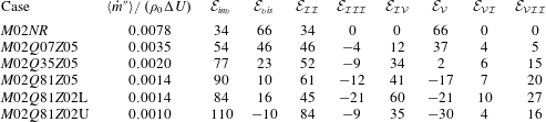
Table 3 summarizes the results for the velocities associated with the entrainment. In this table, the results for the case
 $M02NR$
are found to be similar to the results for incompressible jets and spatially developing mixing layers reported in the literature (Brown & Roshko Reference Brown and Roshko1974; Dimotakis & Brown Reference Dimotakis and Brown1976; Yule Reference Yule1978; Bernal & Roshko Reference Bernal and Roshko1986; Turner Reference Turner1986; Liepmann & Gharib Reference Liepmann and Gharib1992; Babu & Mahesh Reference Babu and Mahesh2004; Westerweel et al.
Reference Westerweel, Fukushima, Pedersen and Hunt2009; Attili & Bisetti Reference Attili and Bisetti2012; Philip & Marusic Reference Philip and Marusic2012; Khashehchi et al.
Reference Khashehchi, Ooi, Soria and Marusic2013; Wolf et al.
Reference Wolf, Holzner, Lüthi, Krug, Kinzelbach and Tsinober2013). Table 3 reveals that increasing the level of heat release does not have a major effect on the boundary entrainment velocity, however, it reduces the local entrainment velocity and induced velocity significantly. It is shown later in § 4.3 that reduction of the local entrainment velocity causes a decrease in the total entrained mass flow rate,
 $\dot{{\mathcal{M}}}$
, of the reacting cases. Thus, from (4.6) it can be seen that the reduction of the entrained mass flow rate in reacting cases while the boundary entrainment velocity remains approximately constant is an indication of a global expansion that occurs inside the turbulent region due to the heat release effects, i.e.
 $\iiint \unicode[STIX]{x2202}\unicode[STIX]{x1D70C}/\unicode[STIX]{x2202}t\,\text{d}{\mathcal{V}}<0$
. In other words, the volume of the turbulent region increases at a larger rate compared to the mass of this region.
Similar to incompressible jets (Yule Reference Yule1978; Liepmann & Gharib Reference Liepmann and Gharib1992; Babu & Mahesh Reference Babu and Mahesh2004; Westerweel et al.
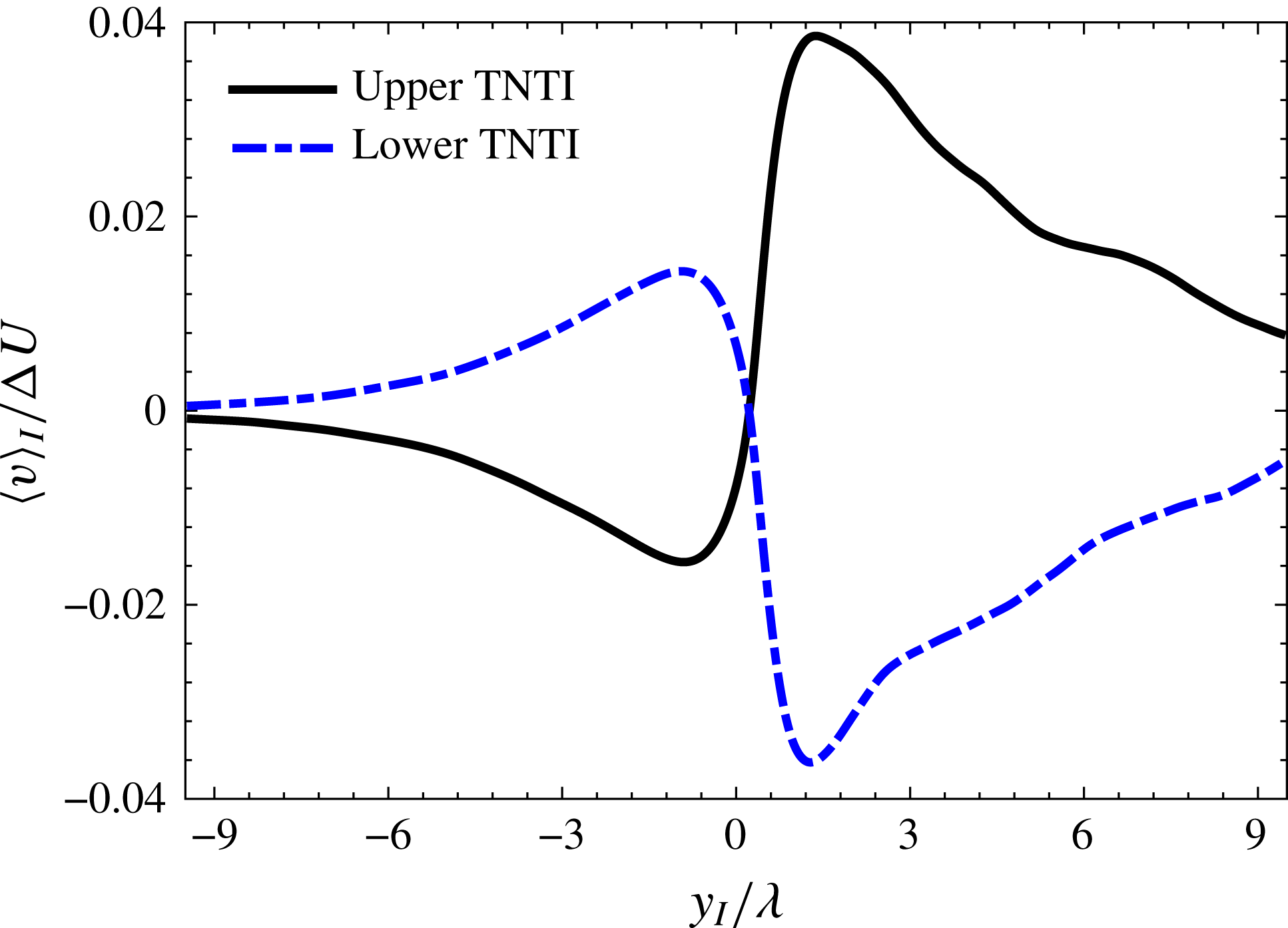
Reference Westerweel, Fukushima, Pedersen and Hunt2009; Philip & Marusic Reference Philip and Marusic2012) and spatially developing mixing layers (Brown & Roshko Reference Brown and Roshko1974; Dimotakis & Brown Reference Dimotakis and Brown1976; Bernal & Roshko Reference Bernal and Roshko1986; Attili & Bisetti Reference Attili and Bisetti2012), table 3 shows that an induced velocity is generated in the non-reacting mixing layer of the current work. Figure 10 depicts the conditional average of
 $v$
in interface coordinate system for upper and lower TNTIs of case
 $M02NR$
. As can be seen, the conditional profile of transverse velocity component in irrotational region resembles the potential flow being induced by larger vortices in the turbulent region, i.e.
 $\langle v\rangle _{I}\propto y_{I}^{-1}$
deep inside the irrotational region and
 $\langle v\rangle _{I}\propto y_{I}$
very close to the TNTI. Therefore, similar to the previous works (Dimotakis & Brown Reference Dimotakis and Brown1976; Yule Reference Yule1978; Liepmann & Gharib Reference Liepmann and Gharib1992; Philip & Marusic Reference Philip and Marusic2012),
 $E_{v}$
is induced primarily by large-scale structures in the flow and helps the nibbling mechanism to become more effective. However, as can be seen in table 3, heat release has an adverse effect on this velocity to the extent that
 $\unicode[STIX]{x0394}E_{v}$
is approximately equal to zero for cases with
 $Q=8.1$
. The decrease of
 $E_{v}$
in the flow can be attributed to the expansion that occurs in the core of turbulent region due to heat release. The expanding turbulent region induces an outward velocity towards the irrotational flow region that counteracts the aforementioned inward induced velocity by the large-scale structures.
Average of the transverse component of velocity,
 $v$
, conditioned on the normal distance from the TNTI,
 $y_{I}$
, for case
 $M02NR$
.
 $\unicode[STIX]{x0394}U$
is the velocity difference of upper and lower streams and
 $\unicode[STIX]{x1D706}$
is the reference value of Taylor length scale.

Table 3 also reveals that the local entrainment velocity normalized by the Kolmogorov velocity,
 $\langle -v_{n}\rangle /u_{\unicode[STIX]{x1D702}}$
, seems to be related to the minimum average density,
 $\bar{\unicode[STIX]{x1D70C}}_{min}/\unicode[STIX]{x1D70C}_{0}$
, in the flow. For example the values of
 $\langle -v_{n}\rangle /u_{\unicode[STIX]{x1D702}}$
for a non-reacting case with
 $M_{c}=1.8$
, reported in our previous work (Jahanbakhshi & Madnia Reference Jahanbakhshi and Madnia2016), and case
 $M02Q07Z05$
, which have similar minimum average density, are very close. Both cases with
 $Q=8.1$
also have similar values of
 $\bar{\unicode[STIX]{x1D70C}}_{min}/\unicode[STIX]{x1D70C}_{0}$
and
 $\langle -v_{n}\rangle /u_{\unicode[STIX]{x1D702}}$
. As is mentioned in § 3, the values of local parameters such as
 $v_{n}$
for upper and lower TNTIs of case
 $M02Q81Z02$
are not similar. Since the purpose of table 3 is to compare the local and integral parameters of entrainment, the average local entrainment velocity of the upper and lower TNTIs is used for all the cases shown here. The local entrained mass flux on each of the TNTIs of case
 $M02Q81Z02$
are studied separately in § 4.2.
At large enough Reynolds numbers for an incompressible turbulence, it is suggested by Corrsin & Kistler (Reference Corrsin and Kistler1955) that local propagation velocity of the turbulence boundary, which is referred to as local entrainment velocity here,
 $v_{n}$
, is proportional to the Kolmogorov velocity scale,
 $u_{\unicode[STIX]{x1D702}}$
. Also a common assumption in the entrainment process is that
 $E_{b}$
is proportional to the typical large-scale velocity in the flow (Morton, Taylor & Turner Reference Morton, Taylor and Turner1956; Turner Reference Turner1986; van Reeuwijk & Holzner Reference van Reeuwijk and Holzner2014; da Silva et al.
Reference da Silva, Hunt, Eames and Westerweel2014a
). The largest eddies in the flow are characterized by the length scale
 ${\mathcal{L}}$
, which is of the order of the flow scale, and their characteristic velocity,
 $u_{{\mathcal{L}}}$
, is of the order of the root-mean-square (r.m.s.) turbulence intensity,
 $\sqrt{2k/3}$
, where
 $k$
is the turbulent kinetic energy (Pope Reference Pope2000). Consequently, the ratio of the local entrainment velocity to the boundary entrainment velocity is given by (Pope Reference Pope2000; van Reeuwijk & Holzner Reference van Reeuwijk and Holzner2014)
 $$\begin{eqnarray}\frac{v_{n}}{E_{b}}\propto \frac{u_{\unicode[STIX]{x1D702}}}{u_{{\mathcal{L}}}}\sim Re_{{\mathcal{L}}}^{-1/4},\end{eqnarray}$$
where
 $Re_{{\mathcal{L}}}\equiv (u_{{\mathcal{L}}}{\mathcal{L}})/\unicode[STIX]{x1D708}$
is the Reynolds number of the largest eddies in the flow. The proportionality shown in (4.8) holds well for case
 $M02NR$
, however as the level of heat release increases the ratio
 $v_{n}/E_{b}$
is no longer proportional to
 $Re_{{\mathcal{L}}}^{-1/4}$
. To extend Kolmogorov’s phenomenology for flows with variable density, it is suggested that a density-weighted velocity,
 $\unicode[STIX]{x1D70C}^{\unicode[STIX]{x1D6FC}}\boldsymbol{u}$
with
 $0\leqslant \unicode[STIX]{x1D6FC}\leqslant 1$
, provides scaling laws that takes into account the compressibility (Kida & Orszag Reference Kida and Orszag1990; Kritsuk et al.
Reference Kritsuk, Norman, P. and Wagner2007; Schmidt, Federrath & Klessen Reference Schmidt, Federrath and Klessen2008; Aluie Reference Aluie2013; Wang et al.
Reference Wang, Yang, Shi, Xiao, He and Chen2013).
 $\unicode[STIX]{x1D6FC}\sim 1$
seems to yield the best scaling for the cases of the present study. Using this scaling, it can be obtained that
 $$\begin{eqnarray}\frac{v_{n}}{E_{b}}\propto \frac{\bar{\unicode[STIX]{x1D70C}}_{min}}{\unicode[STIX]{x1D70C}_{0}}Re_{{\mathcal{L}}}^{-1/4},\end{eqnarray}$$
where
 $\unicode[STIX]{x1D70C}_{0}$
is the density of the outside irrotational flow and
 $\bar{\unicode[STIX]{x1D70C}}_{min}$
is the minimum average density of the flow on homogeneous planes, which is reached at the average location of the flame for reacting cases and on the midplane for the non-reacting case. The proportionality in (4.9) holds for all the cases in the current work. Table 3 shows the values of the terms in (4.8) and (4.9). In this table,
 ${\mathcal{L}}$
is considered to be equal to
 $(l_{x}+l_{z}+\unicode[STIX]{x1D6FF}_{\unicode[STIX]{x1D703}})/3$
, where
 $l_{x}$
and
 $l_{z}$
are the integral length scales in the
 $x$
and
 $z$
directions and
 $\unicode[STIX]{x1D6FF}_{\unicode[STIX]{x1D703}}$
is the momentum thickness. For this choice of
 ${\mathcal{L}}$
,
 $v_{n}/E_{b}$
and
 $(\bar{\unicode[STIX]{x1D70C}}_{min}/\unicode[STIX]{x1D70C}_{0})Re_{{\mathcal{L}}}^{-1/4}$
are approximately equal, however, they may not become equal for other choices of
 ${\mathcal{L}}$
. Thus, the proportionality symbol is used in (4.8) and (4.9).
In our previous work (Jahanbakhshi & Madnia Reference Jahanbakhshi and Madnia2016), it is observed that the proportionality in (4.9) also holds for non-reacting mixing layers with
 $M_{c}$
ranging from 0.2 to 1.8. Therefore, the results of table 3 suggest that at large enough Reynolds numbers the ratio of the local entrainment velocity to the boundary entrainment velocity seems to be characterized by the density change in the flow regardless of the source of this change. This indicates that increasing the level of heat release or the convective Mach number reduces the local entrainment, and the rate of this reduction is related to the minimum average density in the flow.
4.2 Average and local mass flux across the TNTI
The mass flow rate associated with nibbling is calculated by multiplying the entrained mass flux with the surface area of the TNTI (see (4.4)). The entrained mass flux and the terms contributing to it, can be computed using enstrophy transport equation (Jahanbakhshi & Madnia Reference Jahanbakhshi and Madnia2016). The local entrained mass flux of the irrotational flow into the turbulent region at the TNTI can be written as
 $$\begin{eqnarray}{\dot{m}}^{\prime \prime }=-\unicode[STIX]{x1D70C}v_{n},\end{eqnarray}$$
where
 $v_{n}$
is the local entrainment velocity, defined in (4.3). In this equation, positive
 ${\dot{m}}^{\prime \prime }$
corresponds to the flux of the irrotational flow into the rotational region.
 ${\dot{m}}^{\prime \prime }>0$
is usually referred to as entrainment and
 ${\dot{m}}^{\prime \prime }<0$
is referred to as detrainment. The non-dimensional form of the enstrophy transport equation in a compressible flow is
 $$\begin{eqnarray}\displaystyle & & \displaystyle \underbrace{\frac{\text{D}\unicode[STIX]{x1D6FA}}{\text{D}t}}_{\unicode[STIX]{x1D6FA}_{{\mathcal{I}}}}=\underbrace{2\unicode[STIX]{x1D74E}\boldsymbol{\cdot }\left[\unicode[STIX]{x1D74E}\boldsymbol{\cdot }\unicode[STIX]{x1D735}\boldsymbol{{\mathcal{U}}}\right]}_{\unicode[STIX]{x1D6FA}_{{\mathcal{I}}{\mathcal{I}}}}\underbrace{-2\unicode[STIX]{x1D6E9}\unicode[STIX]{x1D6FA}}_{\unicode[STIX]{x1D6FA}_{{\mathcal{I}}{\mathcal{I}}{\mathcal{I}}}}+\underbrace{\frac{2}{\unicode[STIX]{x1D70C}^{2}}\unicode[STIX]{x1D74E}\boldsymbol{\cdot }\left(\unicode[STIX]{x1D735}\unicode[STIX]{x1D70C}\times \unicode[STIX]{x1D735}p\right)}_{\unicode[STIX]{x1D6FA}_{{\mathcal{I}}{\mathcal{V}}}}\nonumber\\ \displaystyle & & \displaystyle \quad \quad +\,\underbrace{\frac{2\unicode[STIX]{x1D708}}{Re}\unicode[STIX]{x1D74E}\boldsymbol{\cdot }\unicode[STIX]{x1D6FB}^{2}\unicode[STIX]{x1D74E}}_{\unicode[STIX]{x1D6FA}_{{\mathcal{V}}}}+\underbrace{\frac{2\unicode[STIX]{x1D708}}{\unicode[STIX]{x1D70C}Re}\unicode[STIX]{x1D74E}\boldsymbol{\cdot }\left[\unicode[STIX]{x1D735}\unicode[STIX]{x1D70C}\times \left(\unicode[STIX]{x1D735}\times \unicode[STIX]{x1D74E}-\frac{4}{3}\unicode[STIX]{x1D735}\unicode[STIX]{x1D6E9}\right)\right]}_{\unicode[STIX]{x1D6FA}_{{\mathcal{V}}{\mathcal{I}}}}\nonumber\\ \displaystyle & & \displaystyle \quad \quad +\,\underbrace{\frac{2\unicode[STIX]{x1D74E}}{Re}\boldsymbol{\cdot }\!\left[\unicode[STIX]{x1D735}\times \left\{\!\frac{2\unicode[STIX]{x1D735}\unicode[STIX]{x1D707}\boldsymbol{\cdot }\unicode[STIX]{x1D735}\boldsymbol{{\mathcal{U}}}}{\unicode[STIX]{x1D70C}}-\frac{2\unicode[STIX]{x1D6E9}\unicode[STIX]{x1D735}\unicode[STIX]{x1D707}}{3\unicode[STIX]{x1D70C}}+\frac{\unicode[STIX]{x1D735}\unicode[STIX]{x1D707}\times \unicode[STIX]{x1D74E}}{\unicode[STIX]{x1D70C}}\!\right\}-\frac{\unicode[STIX]{x1D735}\unicode[STIX]{x1D707}}{\unicode[STIX]{x1D70C}}\times \left(\!\unicode[STIX]{x1D735}\times \unicode[STIX]{x1D74E}-\frac{4}{3}\unicode[STIX]{x1D735}\unicode[STIX]{x1D6E9}\!\right)\!\right]}_{\unicode[STIX]{x1D6FA}_{{\mathcal{V}}{\mathcal{I}}{\mathcal{I}}}},\nonumber\\ \displaystyle & & \displaystyle\end{eqnarray}$$
where
 $\boldsymbol{{\mathcal{U}}}$
,
 $\unicode[STIX]{x1D74E}=\unicode[STIX]{x1D735}\times \boldsymbol{{\mathcal{U}}}$
,
 $\unicode[STIX]{x1D6E9}=\unicode[STIX]{x1D735}\boldsymbol{\cdot }\boldsymbol{{\mathcal{U}}}$
and
 $\unicode[STIX]{x1D6FA}=\unicode[STIX]{x1D74E}\boldsymbol{\cdot }\unicode[STIX]{x1D74E}$
are the velocity vector, the vorticity vector, divergence of velocity referred to as dilatation and enstrophy respectively. In (4.11), the term on the left-hand side is the total variation of the enstrophy at each point in the flow while moving with the fluid element. On the right-hand side, term
 $\unicode[STIX]{x1D6FA}_{{\mathcal{I}}{\mathcal{I}}}$
represents stretching/compression of the vortex lines, which increases/decreases the enstrophy. Term
 $\unicode[STIX]{x1D6FA}_{{\mathcal{I}}{\mathcal{I}}{\mathcal{I}}}$
represents the decrease/increase of the enstrophy due to fluid expansion/compression. This term is referred to as the dilatation term in this paper. Term
 $\unicode[STIX]{x1D6FA}_{{\mathcal{I}}{\mathcal{V}}}$
corresponds to the generation of the enstrophy due to the baroclinic torque caused by the misalignment of the density and the pressure gradients. Term
 $\unicode[STIX]{x1D6FA}_{{\mathcal{V}}}$
is the viscous diffusion plus viscous dissipation of the enstrophy (
 $2\unicode[STIX]{x1D74E}\boldsymbol{\cdot }\unicode[STIX]{x1D6FB}^{2}\unicode[STIX]{x1D74E}=\unicode[STIX]{x1D6FB}^{2}\unicode[STIX]{x1D6FA}-2\unicode[STIX]{x1D735}\unicode[STIX]{x1D74E}:\unicode[STIX]{x1D735}\unicode[STIX]{x1D74E}$
). Term
 $\unicode[STIX]{x1D6FA}_{{\mathcal{V}}{\mathcal{I}}}$
is the generation of the enstrophy due to a torque generated by the variation of the shear stress in the density-gradient field. This term is referred to as shear stress–density-gradient term in this paper. Term
 $\unicode[STIX]{x1D6FA}_{{\mathcal{V}}{\mathcal{I}}{\mathcal{I}}}$
is the change of enstrophy due to the variation of viscosity. Using (4.3) and (4.11), equation (4.10) can be rewritten as
 $$\begin{eqnarray}\displaystyle & & \displaystyle {\dot{m}}^{\prime \prime }=\underbrace{\frac{2\unicode[STIX]{x1D70C}}{|\unicode[STIX]{x1D735}\unicode[STIX]{x1D6FA}|}\unicode[STIX]{x1D74E}\boldsymbol{\cdot }\left(\unicode[STIX]{x1D74E}\boldsymbol{\cdot }\unicode[STIX]{x1D735}\boldsymbol{{\mathcal{U}}}\right)}_{{\dot{m}}_{{\mathcal{I}}{\mathcal{I}}}^{\prime \prime }}\underbrace{-\frac{2\unicode[STIX]{x1D70C}}{|\unicode[STIX]{x1D735}\unicode[STIX]{x1D6FA}|}\unicode[STIX]{x1D6E9}\unicode[STIX]{x1D6FA}}_{{\dot{m}}_{{\mathcal{I}}{\mathcal{I}}{\mathcal{I}}}^{\prime \prime }}+\underbrace{\frac{2}{\unicode[STIX]{x1D70C}|\unicode[STIX]{x1D735}\unicode[STIX]{x1D6FA}|}\unicode[STIX]{x1D74E}\boldsymbol{\cdot }\left(\unicode[STIX]{x1D735}\unicode[STIX]{x1D70C}\times \unicode[STIX]{x1D735}p\right)}_{{\dot{m}}_{{\mathcal{I}}{\mathcal{V}}}^{\prime \prime }}\nonumber\\ \displaystyle & & \displaystyle ~~~+\,\underbrace{\frac{2\unicode[STIX]{x1D707}}{Re|\unicode[STIX]{x1D735}\unicode[STIX]{x1D6FA}|}\unicode[STIX]{x1D74E}\boldsymbol{\cdot }\unicode[STIX]{x1D6FB}^{2}\unicode[STIX]{x1D74E}}_{{\dot{m}}_{{\mathcal{V}}}^{\prime \prime }}+\underbrace{\frac{2\unicode[STIX]{x1D707}}{\unicode[STIX]{x1D70C}Re|\unicode[STIX]{x1D735}\unicode[STIX]{x1D6FA}|}\unicode[STIX]{x1D74E}\boldsymbol{\cdot }\left[\unicode[STIX]{x1D735}\unicode[STIX]{x1D70C}\times \left(\unicode[STIX]{x1D735}\times \unicode[STIX]{x1D74E}-\frac{4}{3}\unicode[STIX]{x1D735}\unicode[STIX]{x1D6E9}\right)\right]}_{{\dot{m}}_{{\mathcal{V}}{\mathcal{I}}}^{\prime \prime }}\nonumber\\ \displaystyle & & \displaystyle ~~~+\,\underbrace{\frac{2\unicode[STIX]{x1D70C}\unicode[STIX]{x1D74E}}{Re|\unicode[STIX]{x1D735}\unicode[STIX]{x1D6FA}|}\boldsymbol{\cdot }\!\left[\unicode[STIX]{x1D735}\times \!\left\{\!\frac{2\unicode[STIX]{x1D735}\unicode[STIX]{x1D707}\boldsymbol{\cdot }\unicode[STIX]{x1D735}\boldsymbol{{\mathcal{U}}}}{\unicode[STIX]{x1D70C}}-\frac{2\unicode[STIX]{x1D6E9}\unicode[STIX]{x1D735}\unicode[STIX]{x1D707}}{3\unicode[STIX]{x1D70C}}+\frac{\unicode[STIX]{x1D735}\unicode[STIX]{x1D707}\times \unicode[STIX]{x1D74E}}{\unicode[STIX]{x1D70C}}\!\right\}-\frac{\unicode[STIX]{x1D735}\unicode[STIX]{x1D707}}{\unicode[STIX]{x1D70C}}\times \!\left(\!\unicode[STIX]{x1D735}\times \unicode[STIX]{x1D74E}-\frac{4}{3}\unicode[STIX]{x1D735}\unicode[STIX]{x1D6E9}\right)\!\right]}_{{\dot{m}}_{{\mathcal{V}}{\mathcal{I}}{\mathcal{I}}}^{\prime \prime }},\nonumber\\ \displaystyle & & \displaystyle\end{eqnarray}$$
where the effect of inviscid and viscous terms can be studied separately as,
 $$\begin{eqnarray}{\dot{m}}_{inv}^{\prime \prime }={\dot{m}}_{{\mathcal{I}}{\mathcal{I}}}^{\prime \prime }+{\dot{m}}_{{\mathcal{I}}{\mathcal{I}}{\mathcal{I}}}^{\prime \prime }+{\dot{m}}_{{\mathcal{I}}{\mathcal{V}}}^{\prime \prime },\quad {\dot{m}}_{vis}^{\prime \prime }={\dot{m}}_{{\mathcal{V}}}^{\prime \prime }+{\dot{m}}_{{\mathcal{V}}{\mathcal{I}}}^{\prime \prime }+{\dot{m}}_{{\mathcal{V}}{\mathcal{I}}{\mathcal{I}}}^{\prime \prime }.\end{eqnarray}$$
Table 4 shows the values of the average entrained mass flux and contributions of different terms in (4.12) and (4.13) to this flux for different cases. It should be mentioned that the threshold chosen to detect the TNTI affects some of the values reported in this table. However, the trends of how heat release affects the contribution of different terms to the entrained mass flux is not dependent on the threshold value. This is shown in section 2 of the supplementary material of this paper. As can be seen in table 4, increasing the level of heat release results in a decrease in the averaged value of the entrained mass flux. Table 4 reveals that as the level of heat release increases the contribution of the viscous terms to the entrainment decreases, whereas the contribution of the inviscid terms increases. This results in the mass flow rate due to nibbling to become dominated by inviscid effects in reacting cases. The study of the enstrophy transport budgets across the TNTI, shown in Jahanbakhshi (Reference Jahanbakhshi2016), reveals that as the level of heat release increases the shape of the profile of viscous diffusion term changes, resulting in a decrease of the total change of enstrophy in reacting flows near the TNTI. This leads to a reduction in the total contribution of the viscous terms to the entrainment. The results for lower and upper TNTIs of case
 $M02Q81Z02$
are shown separately in table 4 to highlight the effect of flame location. This table shows that the contribution of vortex stretching to entrainment on the TNTI closer to the flame is less than the TNTI farther from it. This is due to the effects of flame/TNTI interaction. This interaction causes the vortical structures to become scarce in the region between the flame and the lower TNTI of case
 $M02Q81Z02$
. Also, as the flame moves towards the TNTI, the gradient of density become larger near the TNTI, shown in figure 9(b). This leads to an increase in the contribution of terms
 ${\dot{m}}_{{\mathcal{I}}{\mathcal{V}}}^{\prime \prime }$
and
 ${\dot{m}}_{{\mathcal{V}}{\mathcal{I}}}^{\prime \prime }$
to entrainment on the lower TNTI compared to the upper TNTI of case
 $M02Q81Z02$
. Table 4 also shows the contribution of the term corresponding to the variation of viscosity to average entrained mass flux,
 ${\mathcal{E}}_{{\mathcal{V}}{\mathcal{I}}{\mathcal{I}}}$
. It can be seen that as the level of heat release increases or the distance between the flame and the TNTI decreases the contribution of this term to the entrained mass flux increases.
Average entrained mass flux,
 $\langle {\dot{m}}^{\prime \prime }\rangle$
, and contribution of different terms of (4.12) and (4.13) to this flux,
 ${\mathcal{E}}_{{\mathcal{N}}}=100\times \langle {\dot{m}}_{{\mathcal{N}}}^{\prime \prime }\rangle /\langle {\dot{m}}^{\prime \prime }\rangle$
.
 $\unicode[STIX]{x1D70C}_{0}$
is the reference value of density, and
 $\unicode[STIX]{x0394}U$
is the velocity difference of upper and lower streams.
 $M02Q81Z02$
L and
 $M02Q81Z02$
U correspond to lower and upper TNTIs of case
 $M02Q81Z02$
respectively.

The parameter
 ${\mathcal{E}}_{{\mathcal{N}}}$
, shown in table 4, can only reveal the average contribution of different terms in (4.12) to the entrained mass flux across the TNTI. For more detailed study of the effect of each term in (4.12) on the local variation of entrained mass flux, it is useful to compute the correlation coefficient between them. Table 5 summarizes these correlation coefficients. This table reveals that for case
 $M02NR$
the entrained mass flux on the TNTI is highly correlated with
 ${\dot{m}}_{{\mathcal{V}}}^{\prime \prime }$
. For the reacting cases, table 5 shows that as the level of heat release increases the local entrained mass flux becomes highly correlated with the baroclinic term. This is consistent with large density change near the TNTI observed in figure 9 for the reacting cases of the present study. The results of tables 4 and 5, indicate that in general nibbling is a viscous dominated mechanism in non-reacting turbulence, whereas it is essentially governed by inviscid terms in reacting flows with high level of heat release.
The correlation coefficient,
 ${\mathcal{C}}$
, of the entrained mass flux,
 ${\dot{m}}^{\prime \prime }$
, with terms in (4.12) on the TNTI.
 $M02Q81Z02$
L and
 $M02Q81Z02$
U correspond to lower and upper TNTIs of case
 $M02Q81Z02$
respectively.

4.3 Total entrained mass flow rate
So far in § 4 only the mass that enters the mixing layer due to nibbling per unit area of the TNTI has been discussed. The second mechanism by which the irrotational flow can become part of the turbulent region is the engulfment. In turbulence, engulfment occurs as large pockets of irrotational flow are drawn into and become surrounded by turbulent flow. These pockets break down into smaller pockets and eventually acquire vorticity.
In the present work, the entrained mass flow rates due to engulfment and nibbling are denoted as
 ${\dot{m}}_{e}$
and
 ${\dot{m}}_{n}$
respectively. As is discussed in the introduction of this paper, using an Eulerian approach it is difficult to calculate
 ${\dot{m}}_{e}$
by directly finding the irrotational pockets embedded inside the turbulent region. In our previous work (Jahanbakhshi & Madnia Reference Jahanbakhshi and Madnia2016), the entrained mass flow rate due to engulfment is estimated by finding the total mass of the irrotational pockets at a time during the self-similar state, and dividing this mass by a characteristic time scale. This characteristic time is the average lifetime of the irrotational pockets inside the turbulent region which is found from a Lagrangian analysis. By using this approach, the contribution of the engulfment to the entrainment is found to be less than 8 % for non-reacting compressible mixing layers. In order to circumvent performing the Lagrangian analysis, in which the computational cost is prohibitively expensive for the reacting cases, an alternate approach is used to compute
 ${\dot{m}}_{e}$
in the present study. In this approach, the total entrained mass flow rate,
 $\dot{{\mathcal{M}}}={\dot{m}}_{n}+{\dot{m}}_{e}$
, into the mixing layer is quantified first. The entrained mass flow rate due to nibbling can also be calculated from (4.4) by using the entrained mass flux and surface area of the TNTI as
 ${\dot{m}}_{n}=\langle {\dot{m}}^{\prime \prime }\rangle _{L}{\mathcal{A}}_{L}+\langle {\dot{m}}^{\prime \prime }\rangle _{U}{\mathcal{A}}_{U}$
, where the subscripts
 $L$
and
 $U$
correspond to the lower and upper TNTIs respectively. The surface area of the TNTI and the entrained mass flux are reported in tables 2 and 4 respectively. Finally, the entrained mass flow rate due to engulfment can be calculated by subtracting the mass flow rate due to nibbling from the total entrained mass flow rate.
In order to find
 $\dot{{\mathcal{M}}}$
, the instantaneous total mass of the turbulent region,
 ${\mathcal{M}}$
, is computed as
 $$\begin{eqnarray}{\mathcal{M}}=\iiint _{\unicode[STIX]{x1D714}\geqslant \unicode[STIX]{x1D714}_{th}}\unicode[STIX]{x1D70C}\,\text{d}x\,\text{d}y\,\text{d}z,\end{eqnarray}$$
where
 $\unicode[STIX]{x1D70C}$
and
 $\unicode[STIX]{x1D714}$
are the instantaneous density and vorticity fields at time
 $t$
, and
 $\unicode[STIX]{x1D714}_{th}$
is the vorticity threshold by which TNTI is detected.
 ${\mathcal{M}}$
approximately changes linearly with time during the self-similar state, not shown here. Thus, the average of the total entrained mass flow rate during the self-similar state is estimated as
 $$\begin{eqnarray}\dot{{\mathcal{M}}}=\frac{{\mathcal{M}}_{t_{f}}-{\mathcal{M}}_{t_{i}}}{t_{f}-t_{i}},\end{eqnarray}$$
where
 $t_{i}$
and
 $t_{f}$
are the initial and final times during the self-similar state. In a temporal configuration as the mixing layer grows,
 $\dot{{\mathcal{M}}}$
,
 ${\dot{m}}_{n}$
and
 ${\dot{m}}_{e}$
increase with time. Therefore, in order to make a meaningful comparison between the cases, these mass flow rates need to be normalized by an appropriate parameter. The total mixing layer mass flow rate,
 $\dot{{\mathcal{Q}}}$
, which is an estimate of the mass flow rate inside the turbulent region in the streamwise direction, is calculated for a compressible mixing layer as
 $$\begin{eqnarray}\dot{{\mathcal{Q}}}=L_{z}\int _{-\infty }^{+\infty }{\mathcal{P}}(t,y)\bar{\unicode[STIX]{x1D70C}}|\tilde{u} |\,\text{d}y,\end{eqnarray}$$
where
 ${\mathcal{P}}(t,y)$
is the probability for a given fluid element in location
 $y$
and time
 $t$
to be between the upper and lower interface envelopes,
 $L_{z}$
is the domain size in the spanwise direction,
 $\bar{\unicode[STIX]{x1D70C}}$
is the density average on homogeneous planes and
 $\tilde{u}$
is the density-weighted (Favre) average of the streamwise velocity on homogeneous planes. As is evident from (4.16), the total mixing layer mass flow rate increases with growth of mixing layer in time. Note that the rate of this increase is related to the entrained mass flow rate, i.e.
 $\dot{{\mathcal{M}}}\sim \dot{{\mathcal{Q}}}_{t+\unicode[STIX]{x1D6FF}t}-\dot{{\mathcal{Q}}}_{t}$
. Thus,
 $\dot{{\mathcal{Q}}}$
is used to normalize the entrained mass flow rates.
Total entrained mass flow rate,
 $\dot{{\mathcal{M}}}$
, mass flow rate due to nibbling,
 ${\dot{m}}_{n}$
, and mass flow rate due to engulfment,
 ${\dot{m}}_{e}$
.
 $\dot{{\mathcal{Q}}}$
is the total mixing layer mass flow rate, defined in (4.16),
 $C_{0}=1.15$
is a constant of proportionality,
 $\unicode[STIX]{x1D6F7}$
is defined in (4.17),
 $\bar{\unicode[STIX]{x1D70C}}_{min}$
is the minimum average density of the flow and
 $\bar{\unicode[STIX]{x1D70C}}_{min,NR}$
is the minimum average density of the corresponding non-reacting case with the same convective Mach number.

The normalized values of the mass flow rates associated with entrainment are reported in table 6. It can be seen that as the level of heat release increases, the normalized values of total entrained mass flow rate decrease. This is mostly due to the decrease of the local entrainment velocity,
 $v_{n}$
, while the surface area of the TNTI does not change significantly. Table 6 also shows that the contribution of the engulfment to entrainment is small for the non-reacting case in accordance with our previous paper (Jahanbakhshi & Madnia Reference Jahanbakhshi and Madnia2016) and previous works on incompressible jets (Mathew & Basu Reference Mathew and Basu2002; Westerweel et al.
Reference Westerweel, Fukushima, Pedersen and Hunt2005, Reference Westerweel, Fukushima, Pedersen and Hunt2009; Hunt et al.
Reference Hunt, Eames, da Silva and Westerweel2011; Taveira et al.
Reference Taveira, Diogo, Lopes and da Silva2013; da Silva et al.
Reference da Silva, Taveira and Borrell2014b
), whereas, for the reacting mixing layers the mass flow rate due to engulfment can constitute up to approximately 40 % of the total entrainment. The increase in the contribution of engulfment to entrainment due to the heat release effects is mostly a consequence of a decrease in the entrained mass flow rate due to nibbling in reacting flows, while the entrained mass flow rate due to engulfment does not change significantly.
The digestion of the large pockets of irrotational flow into the turbulent region is generally an inviscid process. Therefore, the results of this section and § 4.2 indicate that in general entrainment is a viscous dominated process in non-reacting turbulence, whereas it is mostly an inviscid process in reacting flows with high level of heat release.
4.4 Heat release and compressibility effects
As is mentioned in the introduction section, in a recent work by the authors (Jahanbakhshi & Madnia Reference Jahanbakhshi and Madnia2016) the effect of compressibility on the entrainment is examined using a similar approach as the one used here. In this section, the effects of compressibility and heat release on the entrainment are compared with each other. Figures 11 to 13 show the summary of this comparison for the important parameters of entrainment. In these figures
 $M08NR$
,
 $M12NR$
and
 $M18NR$
correspond to the non-reacting cases with
 $M_{c}=0.8$
,
 $1.2$
and
 $1.8$
respectively (Jahanbakhshi & Madnia Reference Jahanbakhshi and Madnia2016). The rest of the cases are described in table 1. Furthermore inspired by several previous works on non-reacting compressible mixing layers and low-speed free shear flows in which the mixing streams have a density difference, an expression is found in this section to model the effects of compressibility and heat release on the total entrained mass flow rate.
Effect of compressibility, (a), and heat release, (b), on the normalized surface area of the TNTI,
 ${\mathcal{A}}/(l_{x}\times l_{z})$
.

The study of the effects of compressibility, shown in Jahanbakhshi & Madnia (Reference Jahanbakhshi and Madnia2016), on the overall growth rate of the mixing layer shows that as the convective Mach number increases, the values of all the velocities associated with the entrainment decrease. While as the level of heat release increases, shown in table 3, the values of the induced velocity and the local entrainment velocity decrease, however, the value of boundary entrainment velocity does not change significantly. As is shown in (4.5), the boundary entrainment velocity,
 $E_{b}$
, is directly proportional to the change of volume of the mixing layer which in turn is related to local expansion or compression that occurs in the flow. Examining the PDFs of the dilatation,
 $\unicode[STIX]{x1D735}\boldsymbol{\cdot }\boldsymbol{{\mathcal{U}}}$
, in the turbulent region for all the cases discussed here, shown in chapter 7 of Jahanbakhshi (Reference Jahanbakhshi2016), reveals that in a non-reacting highly compressible mixing layer the PDF is skewed towards negative values, i.e. compressed regions, whereas in a reacting mixing layer it is skewed towards positive values, i.e. expanded regions. Thus, to answer the question why compressibility and heat release affect
 $E_{b}$
differently, the study of the effect of local dilatation on the flow topology of the turbulent region in compressible and reacting flows can be helpful. This can be a subject of a future work. Based on the results presented in the current work and Jahanbakhshi & Madnia (Reference Jahanbakhshi and Madnia2016), it seems that the ratio of local entrainment velocity to boundary entrainment velocity is proportional to
 $\left(\bar{\unicode[STIX]{x1D70C}}_{min}/\unicode[STIX]{x1D70C}_{0}\right)Re_{{\mathcal{L}}}^{-1/4}$
regardless of the source of the density change, i.e. compressibility or heat release.
Examining the mass flow rate due to nibbling reveals that as the convective Mach number or the level of heat release increases, the average entrained mass flux decreases. This is mainly due to a reduction of the average contribution of the viscous terms to this flux while the average contribution of the inviscid terms increases. The effect of heat release on the entrained mass flow rate due to nibbling is mostly associated with a decrease of the local entrainment velocity while the surface area of the TNTI does not change significantly, whereas the effect of compressibility on the entrainment due to nibbling is related to a decrease in the local entrainment velocity and the surface area of the TNTI, shown in figures 11 and 12.
Effect of compressibility, (a), and heat release, (b), on the normalized local entrainment velocity,
 $\left\langle -v_{n}\right\rangle /u_{\unicode[STIX]{x1D702}}$
.

The difference between the effects of compressibility and heat release on the surface area of the TNTI can be associated with the changes in the local geometry of the TNTI in these cases. The geometrical shape of the TNTI looking from the turbulent region for all the cases discussed here are examined in chapter 3 of Jahanbakhshi (Reference Jahanbakhshi2016). It is shown that in the non-reacting turbulent mixing layers the TNTI isosurface is dominated by the concave shaped surfaces, and as the convective Mach number increases, the probability of finding highly curved concave shaped surfaces on the TNTI decreases, whereas the probability of finding flatter concave and convex shaped surfaces on the TNTI increases. In reacting turbulent mixing layers, as the level of heat release increases the probability of finding highly curved convex shaped surfaces increases, whereas the probability of finding flatter concave shaped surfaces decreases. Consequently the so called minimal surfaces (Hazewinkel Reference Hazewinkel2002) appear more often on the TNTIs of the highly compressible mixing layers compared to the low compressible reacting and non-reacting cases. These surfaces have the least area stretched across a given closed contour, i.e. their surface areas are minimized with respect to certain constraints (Hazewinkel Reference Hazewinkel2002). This indicates that for a given boundary of the mixing layer the surface area of the TNTI reduces with compressibility.
Effect of compressibility, (a), and heat release, (b), on the total entrained mass flow rate and the contribution of nibbling and engulfment to entrainment.

Effect of compressibility, (a), and heat release, (b), on the entrained mass flux due to nibbling,
 ${\dot{m}}^{\prime \prime }$
, and the contribution of viscous,
 ${\dot{m}}_{vis}^{\prime \prime }$
, and inviscid,
 ${\dot{m}}_{inv}^{\prime \prime }$
, terms to this flux, defined in (4.13).

The engulfment mechanism seems to be more important in reacting mixing layers compared to the non-reacting ones, shown in figure 13. This figure shows that in the non-reacting cases the nibbling and engulfment parts of the entrainment decrease due to the effects of compressibility, whereas in reacting cases the entrained mass flow rate due to nibbling decreases as the heat release level increases; however, the entrained mass flow rate due to engulfment does not change appreciably. Based on the results presented here and in Jahanbakhshi & Madnia (Reference Jahanbakhshi and Madnia2016), nibbling is a viscous dominated process in non-reacting compressible turbulence for the range of convective Mach number examined, whereas it is a process which is mostly carried out by inviscid effects in reacting flows with high level of heat release, shown in figure 14. Specifically the contribution of the baroclinic and viscosity variation terms, defined in (4.12), to the average entrainment is more important in reacting mixing layers compared to the non-reacting ones. It is shown in our previous work (Jahanbakhshi Reference Jahanbakhshi2016) that in non-reacting compressible cases the pressure-gradient and density-gradient vectors are most probably aligned in the mixing layer. In these cases only the regions of the flow which are under the influence of intense vorticity structures or shocklets have non-negligible mean baroclinic vorticity generation, as shown in Jahanbakhshi et al. (Reference Jahanbakhshi, Vaghefi and Madnia2015). On the other hand, in reacting flows, the probability of the misalignment between density-gradient and pressure-gradient vectors is of the same order as their alignment, shown in Jahanbakhshi (Reference Jahanbakhshi2016).
As is mentioned in the introduction of this paper, in several previous experimental works (Ricou & Spalding Reference Ricou and Spalding1961; Brown Reference Brown1975; Becker & Yamazaki Reference Becker and Yamazaki1978; Dimotakis Reference Dimotakis1986; Hermanson & Dimotakis Reference Hermanson and Dimotakis1989; Muniz & Mungal Reference Muniz and Mungal2001) on reacting and non-reacting spatial free shear layers in which the two mixing streams have a density difference, it is estimated that the entrainment at different locations along the axis of a free shear layer in the streamwise direction is proportional to the root of density ratio of the two streams. In another work, Dahm (Reference Dahm2005) has proposed that the effects of heat release on the growth rate of exothermic low compressible reacting mixing layers can be characterized by finding an extended density ratio and using this density ratio in the equations obtained for the non-reacting mixing layers. Furthermore, several experimental and computational studies including the non-reacting cases of our previous work (Chinzei et al. Reference Chinzei, Masuya, Komuro, Murakami and Kudou1986; Papamoschou & Roshko Reference Papamoschou and Roshko1988; Samimy & Elliott Reference Samimy and Elliott1990; Debisschop, Chambers & Bonnet Reference Debisschop, Chambers and Bonnet1994; Pantano & Sarkar Reference Pantano and Sarkar2002; Hadjadj, Yee & Sjögreen Reference Hadjadj, Yee and Sjögreen2012; Vaghefi et al. Reference Vaghefi, Nik, Pisciuneri and Madnia2013; Jahanbakhshi & Madnia Reference Jahanbakhshi and Madnia2016) have shown that the growth rate of a non-reacting compressible mixing layer is dependent on the convective Mach number, and the results from these works agree well with the Barone, Oberkampf & Blottner (Reference Barone, Oberkampf and Blottner2006) regression fit that suggests the growth rate of a non-reacting compressible mixing layer is proportional to
 $$\begin{eqnarray}\unicode[STIX]{x1D6F7}=1+\unicode[STIX]{x1D703}_{1}\left(\frac{1}{1+\unicode[STIX]{x1D703}_{2}{M_{c}}^{\unicode[STIX]{x1D703}_{3}}}-1\right),\end{eqnarray}$$
where
 $\unicode[STIX]{x1D703}_{1}=0.5468$
,
 $\unicode[STIX]{x1D703}_{2}=35.53$
and
 $\unicode[STIX]{x1D703}_{3}=8.614$
. Inspired by these results, the normalized total entrained mass flow rate for all the cases of the present study and the cases studied in our previous work (Jahanbakhshi & Madnia Reference Jahanbakhshi and Madnia2016), is shown to be proportional to
 $$\begin{eqnarray}\frac{\dot{{\mathcal{M}}}}{\dot{{\mathcal{Q}}}}\propto \left(\frac{\bar{\unicode[STIX]{x1D70C}}_{min}}{\bar{\unicode[STIX]{x1D70C}}_{min,NR}}\right)^{1/2}\unicode[STIX]{x1D6F7},\end{eqnarray}$$
where
 $\bar{\unicode[STIX]{x1D70C}}_{min}$
is the minimum average density of the flow on homogeneous planes, and
 $\bar{\unicode[STIX]{x1D70C}}_{min,NR}$
is the minimum average density of the corresponding non-reacting case with the same convective Mach number (for the non-reacting cases
 $\bar{\unicode[STIX]{x1D70C}}_{min}/\bar{\unicode[STIX]{x1D70C}}_{min,NR}=1$
). The simulations performed for the present work also included six extra reacting cases for which the results are not reported here in the interest of brevity. These cases are; case 1:
 $M_{c}=0.2$
,
 $Q=8.1$
, and
 $Z_{st}=0.3$
, case 2:
 $M_{c}=0.8$
,
 $Q=3.5$
, and
 $Z_{st}=0.5$
, case 3:
 $M_{c}=0.8$
,
 $Q=8.1$
, and
 $Z_{st}=0.5$
, case 4:
 $M_{c}=1.8$
,
 $Q=0.7$
, and
 $Z_{st}=0.5$
, case 5:
 $M_{c}=1.8$
,
 $Q=3.5$
, and
 $Z_{st}=0.5$
, and case 6:
 $M_{c}=1.8$
,
 $Q=8.1$
, and
 $Z_{st}=0.5$
. The total entrained mass flow rate for these cases is also found to agree well with the proportionality of (4.18). The results from fourteen cases available to us are used to find a constant for the proportionality of (4.18) based on a least square linear fitting, shown in figure 15. The normalized total entrained mass flow rate of different cases of the present study calculated from
 $C_{0}\left(\bar{\unicode[STIX]{x1D70C}}_{min}/\bar{\unicode[STIX]{x1D70C}}_{min,NR}\right)^{1/2}\unicode[STIX]{x1D6F7}$
by using
 $C_{0}=1.15$
as the constant of proportionality is reported in table 6. As can be seen from this table and figure 15, the difference between the total entrained mass flow rates computed from the DNS data and from
 $C_{0}\left(\bar{\unicode[STIX]{x1D70C}}_{min}/\bar{\unicode[STIX]{x1D70C}}_{min,NR}\right)^{1/2}\unicode[STIX]{x1D6F7}$
are less than 10 % for all cases.
Least-square linear fit through DNS data from proportionality of (4.18).
 $\dot{{\mathcal{M}}}$
is the total entrained mass flow rate,
 $\dot{{\mathcal{Q}}}$
is the mixing layer mass flow rate,
 $\unicode[STIX]{x1D6F7}$
is the Barone et al. (Reference Barone, Oberkampf and Blottner2006) regression fit,
 $\bar{\unicode[STIX]{x1D70C}}_{min}$
is the minimum average density of the flow on homogeneous planes,
 $\bar{\unicode[STIX]{x1D70C}}_{min,NR}$
is the minimum average density of the corresponding non-reacting case with the same convective Mach number and
 $C_{0}$
is the slope of the fitted line.

5 Summary of conclusions
DNS of compressible temporally evolving reacting mixing layers have been performed to study the entrainment of the irrotational flow into the turbulent region across the turbulent/non-turbulent interface (TNTI). In order to study the effects of heat release and interaction of the flame with the TNTI on turbulence, several cases with different heat release levels and stoichiometric mixture fractions are chosen for the simulations. The highest level of heat release is opted for to correspond to hydrogen combustion in air. The combustion is mimicked by a one-step irreversible global reaction, and infinitely fast chemistry approximation is used to compute the species mass fractions. Entrainment is studied as two mechanisms; nibbling, considered as the vorticity transport across the TNTI, and engulfment, the drawing of the pockets of the outside irrotational fluid into the turbulent region. A certain threshold of vorticity magnitude is used to identify the TNTI, separating the turbulent and irrotational regions.
Since entrainment is intimately related to the turbulent/non-turbulent interface, some of the characteristics of the TNTI are studied. Similar to previous works on non-reacting incompressible turbulent flows with the presence of the mean shear, i.e. jets, wakes and boundary layers (da Silva et al. Reference da Silva, Hunt, Eames and Westerweel2014a ), the interface layer thickness is found to be approximately equal to one Taylor length scale for non-reacting and reacting compressible mixing layers in which the flame is far from the TNTI. It is observed that as the flame and TNTI become closer, they interact with each other and the interface layer near the TNTI close to the flame becomes thicker. It is shown that increasing the heat release rate seems to have a small effect on the surface area of the TNTI. Also as the flame becomes closer to the TNTI, the surface area of the TNTI decreases.
To study the effect of heat release on the overall growth rate of the mixing layer, the boundary entrainment velocity is computed and compared with the local entrainment velocity. As the level of heat release increases, the values of induced velocity and the local entrainment velocity decrease, however, the value of boundary entrainment velocity does not change significantly. In reacting mixing layers the ratio of local entrainment velocity to boundary entrainment velocity is found to be proportional to
 $\left(\bar{\unicode[STIX]{x1D70C}}_{min}/\unicode[STIX]{x1D70C}_{0}\right)Re_{{\mathcal{L}}}^{-1/4}$
compared to
 $Re_{{\mathcal{L}}}^{-1/4}$
for incompressible non-reacting turbulence.
The mass flow rate due to nibbling is calculated as the product of the entrained mass flux with the surface area of the TNTI. The entrained mass flux and the terms contributing to this flux, is computed by using the enstrophy transport equation, equation (4.11). As the level of heat release increases, the average entrained mass flux decreases, which is mainly due to a reduction of the average contribution of the viscous terms to this flux while the average contribution of the inviscid terms increases. It is observed that the nibbling mechanism is a viscous dominated mechanism in non-reacting turbulence, whereas it is essentially a process governed by inviscid effects in reacting flows with a high level of heat release. The effect of heat release on the entrained mass flow rate due to nibbling is found to be mostly associated with a decrease of the local entrainment velocity while the surface area of the TNTI does not change significantly.
The engulfment mechanism is studied by finding the total entrained mass flow rate into the mixing layer and subtracting the entrained mass flow rate due to nibbling from it. It is shown that the contribution of the engulfment to entrainment is small for the non-reacting mixing layers in accordance with previous works on incompressible jets (Mathew & Basu Reference Mathew and Basu2002; Westerweel et al. Reference Westerweel, Fukushima, Pedersen and Hunt2005, Reference Westerweel, Fukushima, Pedersen and Hunt2009; Hunt et al. Reference Hunt, Eames, da Silva and Westerweel2011; Taveira et al. Reference Taveira, Diogo, Lopes and da Silva2013; da Silva et al. Reference da Silva, Taveira and Borrell2014b ), whereas, for the reacting mixing layers the mass flow rate due to engulfment can constitute up to 40 % of the total entrainment. The increase in contribution of engulfment to entrainment in reacting flows is found to be mainly related to a decrease of entrained mass flow rate due to nibbling while the entrained mass flow rate due to engulfment does not change significantly.
The effect of compressibility on the entrainment, studied in our previous work (Jahanbakhshi & Madnia Reference Jahanbakhshi and Madnia2016), is compared with the effect of heat release on the entrainment, examined here, in § 4.4. It is shown that the normalized total entrained mass flow rate in reacting and non-reacting compressible mixing layers can be estimated from an expression containing the convective Mach number and the density change. This expression is equal to
 $C_{0}\left(\bar{\unicode[STIX]{x1D70C}}_{min}/\bar{\unicode[STIX]{x1D70C}}_{min,NR}\right)^{1/2}\unicode[STIX]{x1D6F7}$
, where
 $C_{0}=1.15$
is a constant of proportionality,
 $\unicode[STIX]{x1D6F7}$
is a regression fit which is only a function of convective Mach number, defined in (4.17),
 $\bar{\unicode[STIX]{x1D70C}}_{min}$
is the minimum average density of the flow on homogeneous planes and
 $\bar{\unicode[STIX]{x1D70C}}_{min,NR}$
is the minimum average density of the flow on homogeneous planes for the corresponding non-reacting case with the same convective Mach number.
Acknowledgements
This work is supported by the National Center for Hypersonic Combined Cycle Propulsion sponsored by AFOSR and NASA under grant FA-9550-09-1-0611. Computational resources are provided by the Center for Computational Research (CCR) at the State University of New York at Buffalo.
Supplementary material and movies
Supplementary material and movies are available at https://doi.org/10.1017/jfm.2018.122.