

1. Introduction
The digital revolution of the music and media technologies since the early 1990s has stimulated an immense growth in the field of sound spatialisation technologies. With many of today’s computer music tools it is possible to render spatial sound scenes for many channels of audio and large numbers of sound sources. Many research centres and performance venues have installed large-scale multichannel systems, offering promising new possibilities for sound spatialisation applications, which require corresponding efforts in the fields of authoring and musical control.
From a compositional point of view, we speak of ‘sound spatialisation’ as soon as the positions of sound sources, the ambience of a room, or any other spatial or acoustic element is taken into account as a musical parameter of a work. While space has probably always played an important role in music composition, the formalisation of space as a structural parameter is a rather recent phenomenon (Harley Reference Harley1994). Stockhausen (Reference Stockhausen1989) stated that spatial configurations are as meaningful as intervals in melody or harmony, and that the consideration of spatial parameters is an integral part of the compositional process. Indeed, even prior to the advent of sound spatialisation technologies as commonly understood today, avant-garde composers in the 1950s had already begun to integrate space as a musical dimension into their pioneering electroacoustic works, taking advantage of the emerging technologies at hand, such as microphones, analogue mixing desks and loudspeakers (e.g. Karlheinz Stockhausen in Kontakte or Gesang der Jünglinge, Pierre Schaeffer in Symphonie pour un homme seul, or Edgar Varèse with Poème électronique).
Now that digital signal processing and musical acoustics are mature and well-established research fields, spatial sound scenes can be realised with a variety of rendering techniques, software tools and hardware setups. The literature reveals a broad spectrum of approaches and implementations for spatial sound rendering: perceptually informed amplitude panning techniques such as Vector Base Amplitude Panning (VBAP) (Pulkki Reference Pulkki1997) or Distance Based Amplitude Panning (DBAP) (Lossius Reference Lossius2007), holophonic techniques aiming at the physical reconstruction of a sound field, such as Wave Field Synthesis (WFS) (Berkhout, de Vries and Vogel Reference Berkhout, de Vries and Vogel1993) or Higher-Order Ambisonics (Daniel Reference Daniel2001), binaural/transaural techniques, and finally hybrid techniques, such as Space Unit Generator (SUG, Moore Reference Moore1983) or Virtual Microphone Control (ViMiC, Braasch Reference Braasch2005).Footnote 1
Each approach, however, relies on specific assumptions about the nature of sound sources, listener and environment, and as a consequence might not be equally well-suited for different musical applications. Considering that electroacoustic works are often performed in multiple venues with different acoustic properties and loudspeaker arrangements, scalability and adaptability of spatialisation systems are also of major importance. To accommodate different scenarios, contexts and configurations, these systems should allow users to conceive spatialisation processes from a more abstract level. While much recent research focuses on strategies for real-time control (see for instance Marshall, Malloch and Wanderley Reference Marshall, Malloch and Wanderley2007) or the development of interchange formats (Peters, Ferguson and McAdams 2007; Kendall, Peters and Geier Reference Kendall, Peters and Geier2008), there have been few attempts to integrate the control of spatialisation into compositional environments. In fact, sound spatialisation is often treated as a post-production technique which is unconnected to the processes dealt with in computer-aided composition, and therefore remains isolated in the corresponding compositional models and applications.
In this paper we present recent works aimed at integrating spatialisation in the computer-aided composition environment OpenMusic (Agon Reference Agon1998; Assayag, Rueda, Laurson, Agon and Delerue Reference Assayag, Rueda, Laurson, Agon and Delerue1999). After a brief discussion of related works (Section 2), we introduce a generic framework for sound synthesis and spatialisation, embedded in this environment (Section 3). The OMPrisma library is described as a structured system where spatialisation processes can be carried out and controlled in a flexible way, in relation to the symbolic compositional models and integrated with sound synthesis processes (Section 4). We present a powerful extension to the sound synthesis and spatialisation frameworks, allowing these two processes to be merged into hybrid structures implementing the concept of spatial sound synthesis (Section 5), and conclude with a number of example applications (Section 6).
2. Related Works
Among the most popular tools used for the compositional control of spatial sound scenes are those commonly referred to as ‘digital audio workstations’ (DAWs). These environments are typically based on the metaphor of a multitrack tape-recorder and allow for automation and non-linear (mostly manual) editing of control parameters separated into a number of tracks. The user, however, has only limited access to the control data, and as the number of sound sources and parameters increases it becomes cumbersome to monitor and manage the complexity of the spatial sound scene. Moreover, it is difficult to link the concrete representations (soundfiles, automation data) to more abstract compositional concepts, as this type of interface doesn’t represent logical relationships.Footnote 2
Real-time audio processing environments, such as Max/MSP (Puckette Reference Puckette1991), PureData (Puckette Reference Puckette1996) or SuperCollider (McCartney Reference McCartney2002) provide frameworks in which control interfaces and rendering algorithms for sound spatialisation can be developed and integrated with more general sound synthesis and/or interactive processes (see for instance Schacher and Kocher Reference Schacher and Kocher2006). The IRCAM Spatialisateur (Jot and Warusfel Reference Jot and Warusfel1995) provides graphical user interfaces in MaxMSP (SpatViewer/SpatOper) which allow the control of numerous low-level parameters via a reduced number of perceptual descriptors such as ‘liveness’, ‘presence’, and the like. Zirkonium (Ramakrishnan, Goßmann and Brümmer 2006) and Beastmulch (Wilson Reference Wilson2008) are examples of large-scale spatialisation systems based on the model of ‘live diffusion’ which allow for the grouping together of sound sources together and for these groups to be controlled individually.
Several research projects focus specifically on higher-level control, abstracting the spatial sound scene description from the rendering techniques (see for example Geier, Ahrens and Spors Reference Geier, Ahrens and Spors2008). The Holo-Edit interface in the Holophon project (Cabaud and Pottier Reference Cabaud and Pottier2002) is an application allowing the high-level control of spatial parameters (trajectories). Conceived as an authoring tool for sound spatialisation, Holo-Edit provides complementary interfaces for viewing or editing of spatial parameters, including a top-view editor, a set of timeline controls and 3D visualisation. In addition, it provides a set of tools for automatic generation and modification of spatial trajectories (Pottier Reference Pottier1998), which is a significant step towards compositional control. Earlier projects, such as MoveInSpace (Todoroff, Traube and Ledent Reference Todoroff, Traube and Ledent1997), also provided advanced features, such as a trajectory generator, room and loudspeaker settings, and correlation of the spatialisation parameters to sound morphological features (some characteristics which will be found in different parts of our work), implemented as an independent control layer on the Ircam Musical Workstation (Lindemann, Starkier and Dechelle Reference Lindemann, Starkier and Dechelle1990). A different approach for the authoring of spatial sound scenes is taken in the MidiSpace (Pachet and Delerue Reference Pachet and Delerue1998) and MusicSpace (Pachet and Delerue Reference Pachet and Delerue2000; Delerue Reference Delerue2004) systems, which provide graphical interfaces allowing the design of spatial sound scenes including MIDI instruments and audio sources. Most notably, these applications include powerful constraint setting and propagation systems allowing the definition of spatial relations between the different sound sources in the scene.
Most control systems, however, focus on a specific model of sound spatialisation (such as surround-mixing, sound-diffusion, etc.). Although we noted the algorithmic possibilities (in Holo-Edit or MoveInSpace) and tools for constraint-setting and propagation (MusicSpace), these features require integration with higher-level programmable environments in order to enable more abstract representations and accommodate different compositional applications. Assayag (Reference Assayag1998) stated that efficient compositional environments should be conceptually close to specialised programming environments: in such compositional contexts, high-level, symbolic tools and processes allow abstracting control data and processes to a set of manageable and musically meaningful representations, while remaining open enough to be used in different contexts by different composers.
OpenSpace (Delerue and Agon Reference Delerue and Agon1999) was an original attempt at integrating the MusicSpace control system in the computer-aided composition environment OpenMusic. Visual programs allowed defining a spatial setup for MusicSpace sound sources and incrementally adding constraints, while the maquette interface was used to control the unfolding of this process in time. Another project carried out in OpenMusic is OMSpat (Nouno and Agon Reference Nouno and Agon2002), a library for the control of the Spatialisateur. In OMSpat an array of sound sources, trajectories and room parameters could be created from algorithmically (or manually) defined curves and parameters. This array was then formatted as a parameter file for a specific Spatialisateur control application that could reproduce the spatial sound scene using two, four or eight speakers, or via binaural rendering. Although the number of simultaneous sound sources and the temporal resolution of the control data were limited, as well as the number of simultaneous sound sources and the temporal resolution of the control-data, the ability to script trajectories and spatial parameters allowed the user to establish structural relationships between spatialisation and other symbolic data and processes defined in the computer-aided composition environment. This project has recently been generalised and extended, introducing new 3D-trajectory objects and tools for formatting output for external environments (Bresson, Agon and Schumacher 2010). Some similarities can also be found in the works we present in this paper, which inherit much of the control paradigms and structures from the same type of objects (matrices: see Section 3).
As discussed below, we approach the control of sound spatialisation by considering spatial attributes as additional parameters in a sound synthesis framework, whether they relate to micro-level sound synthesis components (such as partials or grains) or to pre-existing sound sources. This approach, embedded in a high-level control environment, allows us to extend the common model of sound source spatialisation to the more general concept of spatial sound synthesis, and to generalise some of the techniques for time-domain or frequency-domain spatial distributions (presented for instance in Topper, Burtner and Serafin 2002; Kim-Boyle Reference Kim-Boyle2008), within a symbolic and programmable compositional context.
3. A generic Framework for the Control of Sound Spatialisation
3.1. The computer-aided composition environment: OpenMusic
OpenMusic (OM) is a visual programming language for music composition based on Common Lisp/CLOS (Gabriel, White and Bobrow 1991). This environment allows the graphical design of programs by patching together functional components, and provides high-level musical interfaces such as scores and other graphical editors. It has been used to develop numerous musical works, constituting a powerful and efficient framework for the creation of complex musical structures related to various compositional approaches (Agon, Assayag and Bresson Reference Agon, Assayag and Bresson2006; Bresson, Agon and Assayag Reference Bresson, Agon and Assayag2008). Additional development in OpenMusic has involved the integration of sound processing, analysis and synthesis tools, and led to a renewed conception of sound representations in the framework of computer-aided compositional models (Bresson and Agon Reference Bresson and Agon2007).
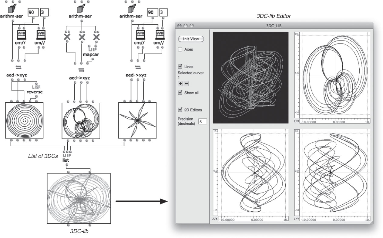
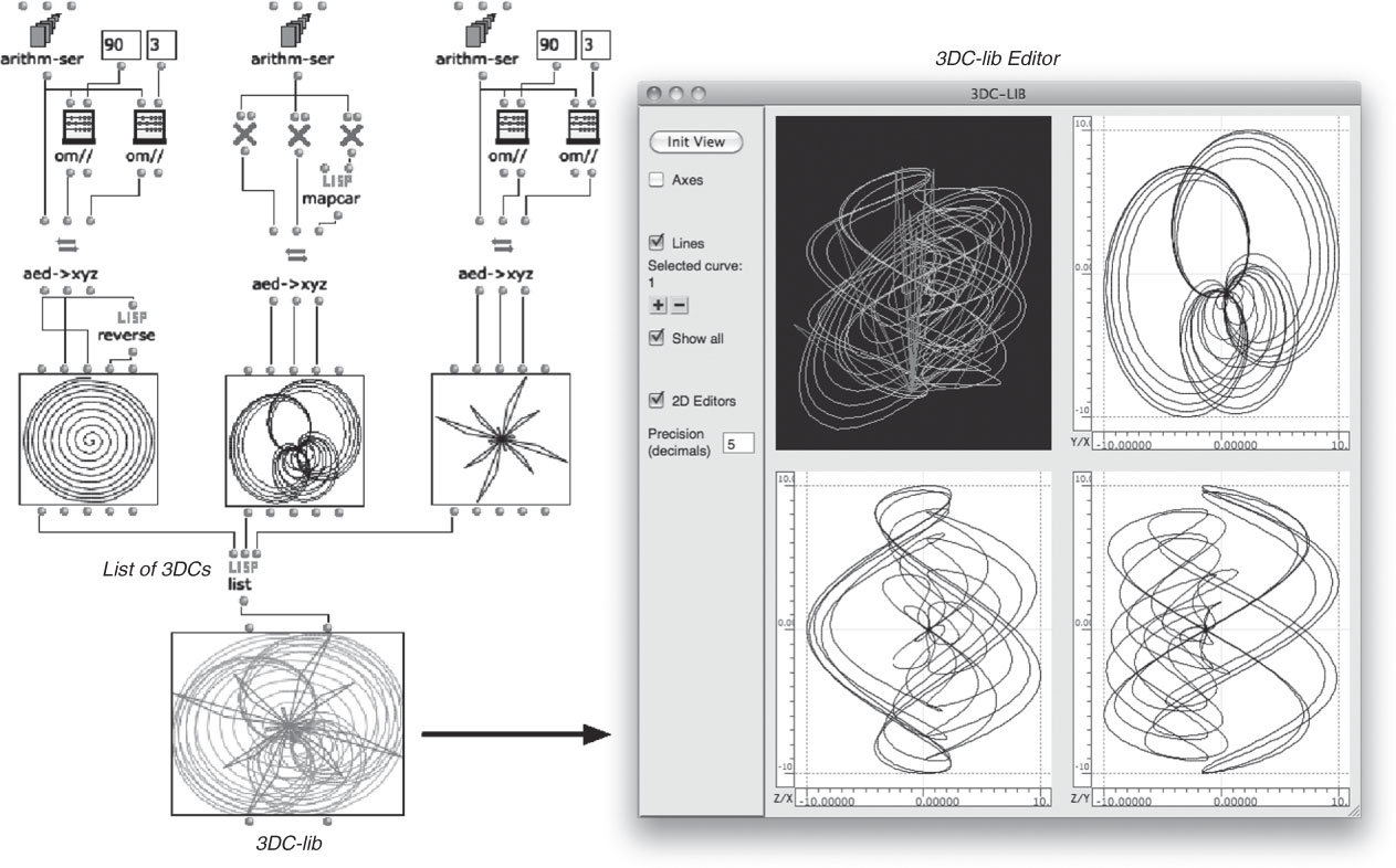
Integrating the control of sound spatialisation into the conceptual framework of a computer-aided composition environment introduces new possibilities: spatialisation parameters, as any other musical data, can be devised and determined using algorithms and programming interfaces, hence in close relation with associated processes. OpenMusic provides a number of geometrical objects such as breakpoint- and 3D-curves (BPC/3DC) representing abstract spatial configurations defined as sequences of points. Temporal information can be explicitly specified (which turns curves into trajectories), or kept implicit and interpreted according to a given context. These objects can be generated and transformed by algorithmic processes in the programming environment or visualised and edited manually using graphical editors. Figure 1 shows an example for the algorithmic generation of 3D-curves by visual programs.
Generation of 3D-curves via visual programs in OM. The 3DC-lib box is a set of 3DC objects. The data can be visualised and edited in graphical editors.
3.2. Sound synthesis and spatialisation: OMChroma/OMPrisma
OMChroma (Agon, Stroppa and Assayag Reference Agon, Stroppa and Assayag2000) is a compositional framework for the control of sound synthesis in OpenMusic, based on Marco Stroppa’s Chroma system (Stroppa Reference Stroppa2000). This framework provides a set of classes (in terms of object-oriented programming) referring to underlying sound synthesis processes. Each class is associated with a digital signal processing (DSP) patch, currently in the form of a Csound instrument (Boulanger Reference Boulanger2000). The parameters of these instruments (called p-fields in Csound) are detected and matched to corresponding slots of the class, which can be instantiated in OpenMusic’s visual programs. Accordingly, the graphical representation of an OMChroma class (called a box) has a number of inlets corresponding to the underlying sound synthesis parameters in the Csound instrument. OMChroma includes a large library of classes, ranging from basic (e.g. additive, granular, FM) to more complex sound synthesis algorithms. This library is user-extensible, and new classes can easily be defined from existing Csound instruments.
OMChroma classes are matrix structures, instantiated with a given number of ‘components’ (represented as columns). Each row corresponds to a slot of the class (i.e. to the related synthesis parameter in the Csound instrument). A matrix can include arbitrary numbers of components, describing vectors of parameter-values for the underlying synthesis instrument, which can be controlled via high-level and symbolic means and subjected to compositional processes. When the matrix is ‘synthesised’ (i.e. rendered into an audio file) a Csound score is generated from the 2D data structure: each component in the matrix (a column with a value for each synthesis parameter) corresponds to an event in the score (see Stroppa Reference Stroppa2000 for a detailed discussion).
OMPrisma is a library providing a set of matrix classes corresponding to spatial sound rendering instruments (see Section 4). The OMPrisma classes extend the OMChroma matrix, and therefore benefit from the same expressive power and data structures used in the control of sound synthesis processes. The computed matrix contents depend on the type of the supplied data and on the number of components: a single value, for instance, means that all components have the same value for a given parameter; lists of values are taken literally or repeated cyclically until the number of elements matches the number of components; breakpoint-functions are sampled over the number of components; and mathematical/functional expressions (defined as Lisp functions or visual programs) are evaluated individually for each component. Once instantiated, the contents of a matrix can be visualised and edited manually as a 2D array using a graphical editor.
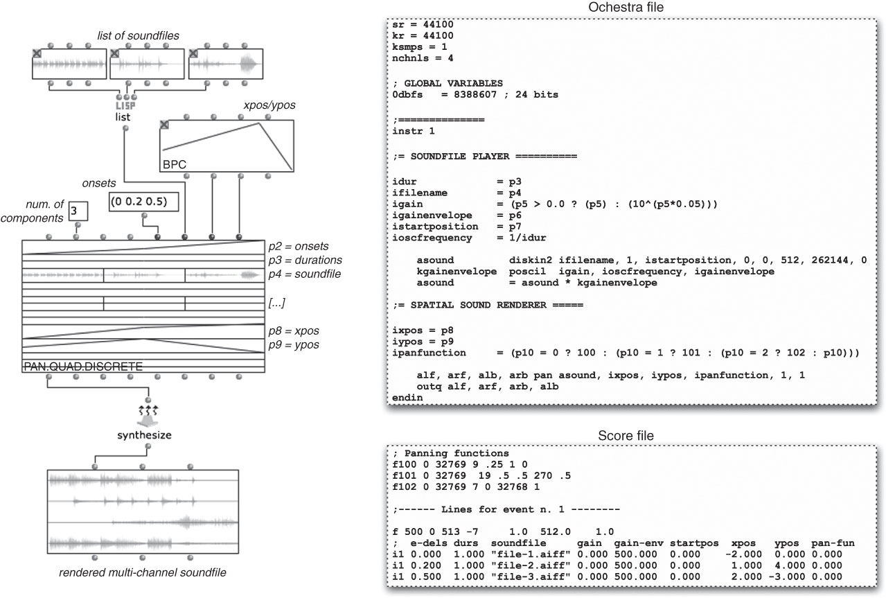
Figure 2 shows a basic sound spatialisation process carried out in OMPrisma. A set of monaural soundfiles is spatialised and rendered into a multichannel file for quadrophonic reproduction using the class pan.quad.discrete from the OMPrisma class-library.
Sound source spatialisation with OMPrisma. Left: the patch in OpenMusic. Right: the generated Csound orchestra and score files.
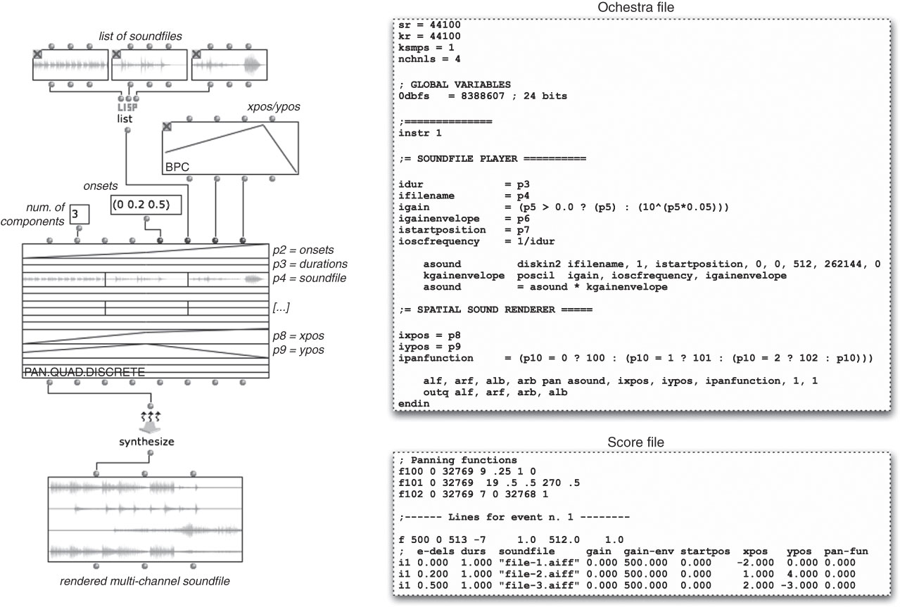
The body of the instrument in the orchestra file of figure 2 (from instr1 to endin) is copied from the pan.quad.discrete class. The synthesize function formats the values of the components in the matrix into Csound score statements (i.e. turning the columns into rows). Most values here are numbers (except the file names used for p4, which are derived from the soundfiles in the OM patch). When continuously changing values are required, for example for describing transitions or envelopes, breakpoint-function objects can be used, which are internally converted into Csound tables.
Note that not all parameters (p-fields in the Csound orchestra) are explicitly specified in the OM patch. The matrix boxes allow the user to selectively display or hide the different slot inlets of a class, whereby unspecified (i.e. hidden) slots are set to default values. In figure 2, only the slots onsets, soundfile, xpos and ypos, corresponding to p2, p4, p8 and p9, respectively, are specified to control the spatialisation process. The default value for the slot gain-envelope, for example, is 500 (a Csound table identifier), which is set for p6 as no value is specified in the OM patch. Similarly, the three ‘panning function tables’ (visible at the top of the score file in figure 2) are defined inside the class PAN.QUAD.DISCRETE, and function as presets, which can be referred to via numerical indices in the Csound score. This way irrelevant or redundant information is hidden from the user, making for a more ergonomic and context-sensitive interface.
As in the case of sound synthesis processes, the dynamic instantiation of multiple Csound instruments (corresponding to the components of a matrix) yields a virtually unlimited polyphony for the spatial sound rendering process. In this perspective, a matrix can be regarded as a generic data structure for the description of spatial sound scenes with arbitrary numbers of sound sources, possibly controlled independently, using common rules, control data or algorithms.
It is also possible to devise a spatialisation process using multiple matrices (i.e. synthesising a list of matrices instead of a single one). If the matrices correspond to different classes, the respective instruments are gathered in a single orchestra file and identified by instrument number (instr1, instr2, …). Each matrix can also be assigned a global onset-time, allowing it to be considered as a temporal ‘event’ in a larger-scale time structure.
4. OMPrisma
OMPrisma is implemented as an extensible framework comprising a library of classes for spatial sound rendering (Section 4.1), a library of tools and functions for generation and manipulation of spatialisation parameters (Section 4.2), and an external standalone application (titled Multiplayer) for decoding and diffusion of the rendered multichannel audio formats (Section 4.3).
Several studies have documented a great variety of compositional approaches for sound spatialisation (see for example Harley Reference Harley1994), and it is unlikely that a specific spatial sound rendering technique will satisfy every artist’s needs. A more sensible solution is to provide an abstraction layer which separates the spatial sound scene description from its rendering, and leave it to the user which spatial sound rendering technique is most suitable for a given purpose.
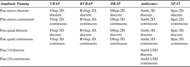
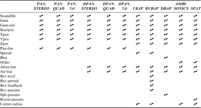
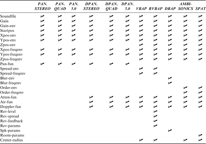
The OMPrisma class-library provides a palette of spatial sound rendering instruments, implementing different spatial sound rendering techniques. Currently available are classes for stereo, quadrophonic and 5.0 (ITU) panning, Vector Base Amplitude Panning (VBAP), Reverberated VBAP (RVBAP), Distance-based Amplitude Panning (DBAP), Higher-Order Ambisonics, and a mixed-order Ambisonics system with optional simulation of room-acoustics. Table 1 gives an overview of implemented spatial sound rendering concepts and respective classes.
Spatial sound rendering concepts and respective classes in OMPrisma

Dynamically changing values, such as envelopes or trajectories (i.e. ‘spatial glissandi’) can be described both in terms of successions of discrete, ‘granular’ positions or as a single continuous movement (consider for example the notion of a glissando on a piano vs. a string instrument). In (Harley Reference Harley1998) the author discusses the difference between ‘discrete’ or ‘stepwise proceeding’ spatial movements (dating back to the Venetian school of polychorality in the late renaissance), and ‘continuous’ motion (introduced in instrumental and electronic music of the post-war avant-garde). We adopted this notion in that every OMPrisma class is available in a dedicated version for discrete and continuous control, respectively.
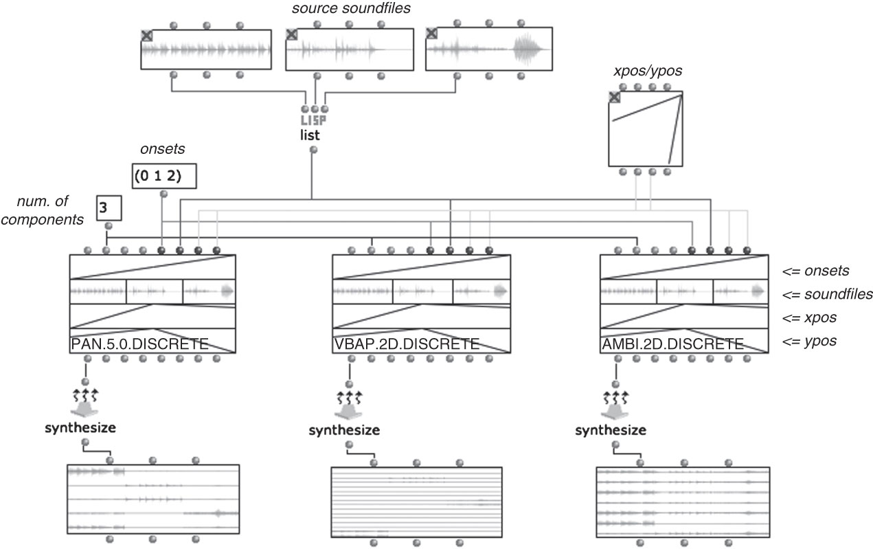
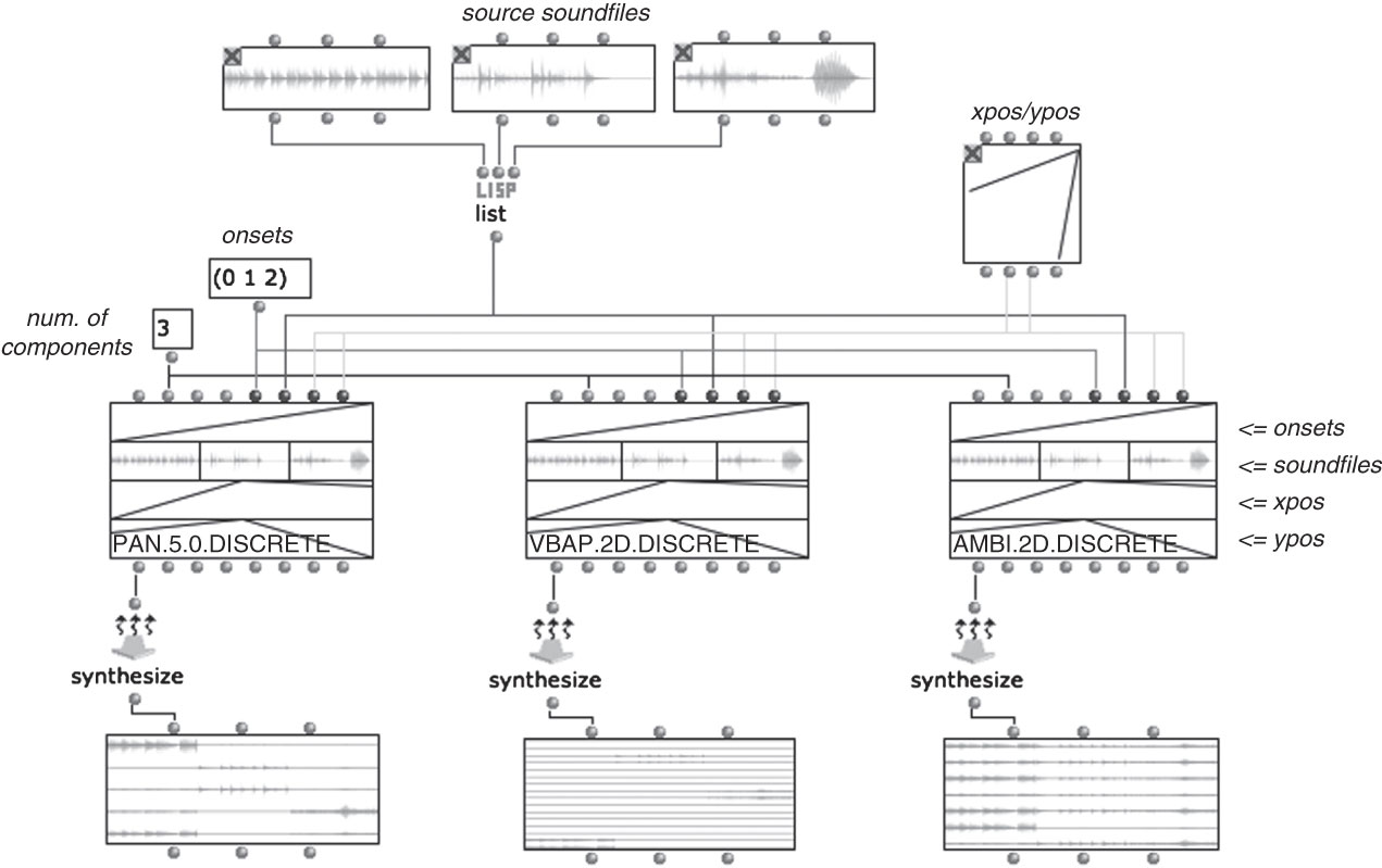
The separation of the spatial sound scene description from its rendering and reproduction offers many advantages (see Peters, Lossius, Schacher, Baltazar, Bascou and Place 2009). For example, it allows the user to rapidly exchange a given spatial sound rendering engine with another one without affecting the other components. It further facilitates modifications or extensions at the renderer level (i.e. Csound instruments), since the DSP implementation can be modified independently as long as it provides the same interface to the environment. Moreover, the use of an external real-time application for decoding and diffusion (the Multiplayer) will provide the flexibility of adapting the reproduction of a spatial sound scene to a given environment. Figure 3 shows an example of 3 OMPrisma classes rendering the same spatial sound scene using different techniques.
The same spatial sound scene realised with different spatial sound rendering techniques: 5.0 (ITU) panning, VBAP and higher-order Ambisonics.
4.1. Spatial sound rendering
OMPrisma employs the Csound language as a spatial sound rendering engine, which allows for sample-synchronous control of all parameters, high-resolution processing and unlimited polyphony. Note that the same matrix control structures may as well be used and formatted for another synthesis engine, or written into external interchange format files (see e.g. Stroppa Reference Stroppa2000; Bresson et al. Reference Bresson, Agon and Schumacher2010). In order to easily maintain, modify and extend the collection of spatial sound rendering instruments, they have been implemented following a modular design. Common functionality is encapsulated into modules (code-snippets) and re-used across the different instruments, such as the soundfile-player, or source pre-processing modules. In the following section we will discuss some of the implementation-specific details.
4.1.1. Dynamic instrument configuration
Many spatialisation algorithms are capable of driving various loudspeaker configurations and numbers of output channels. The OMChroma system allows for the writing of global statements into Csound orchestra files before the instrument definition, which permits dynamic changes to the output configuration without the need to modify the original instrument’s body.Footnote 3 Accordingly, a single OMPrisma class (implementing a specific spatial sound rendering technique) can be used for various loudspeaker setups and output channels.
4.1.2. Source pre-processing
For classes implementing intensity-based panning techniques we have developed source pre-processing modules for the rendering of perceptual cues to support the impression of distance and motion of a sound source. The effect of air absorption is simulated with a second-order Butterworth lowpass filter with variable cut-off frequency. An attenuation-module accounts for the decrease of a sound source’s amplitude as a function of distance. Doppler shifts are simulated with a moving write-head delay line with high quality interpolation.
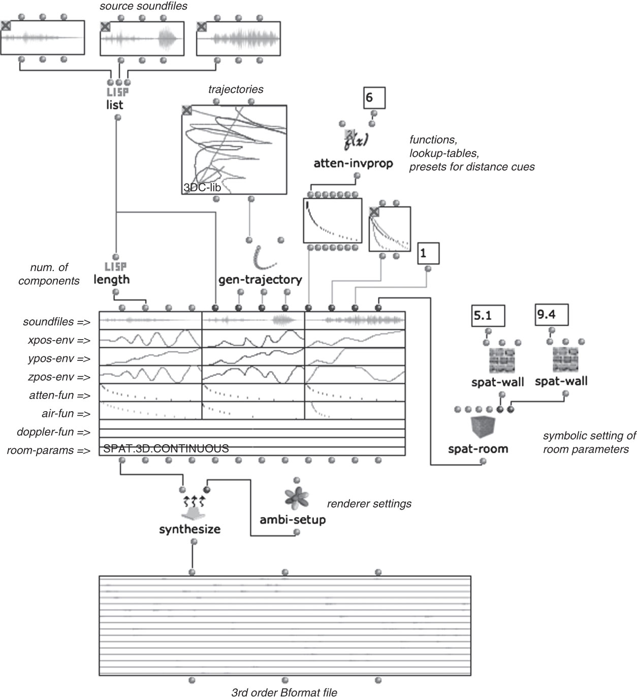
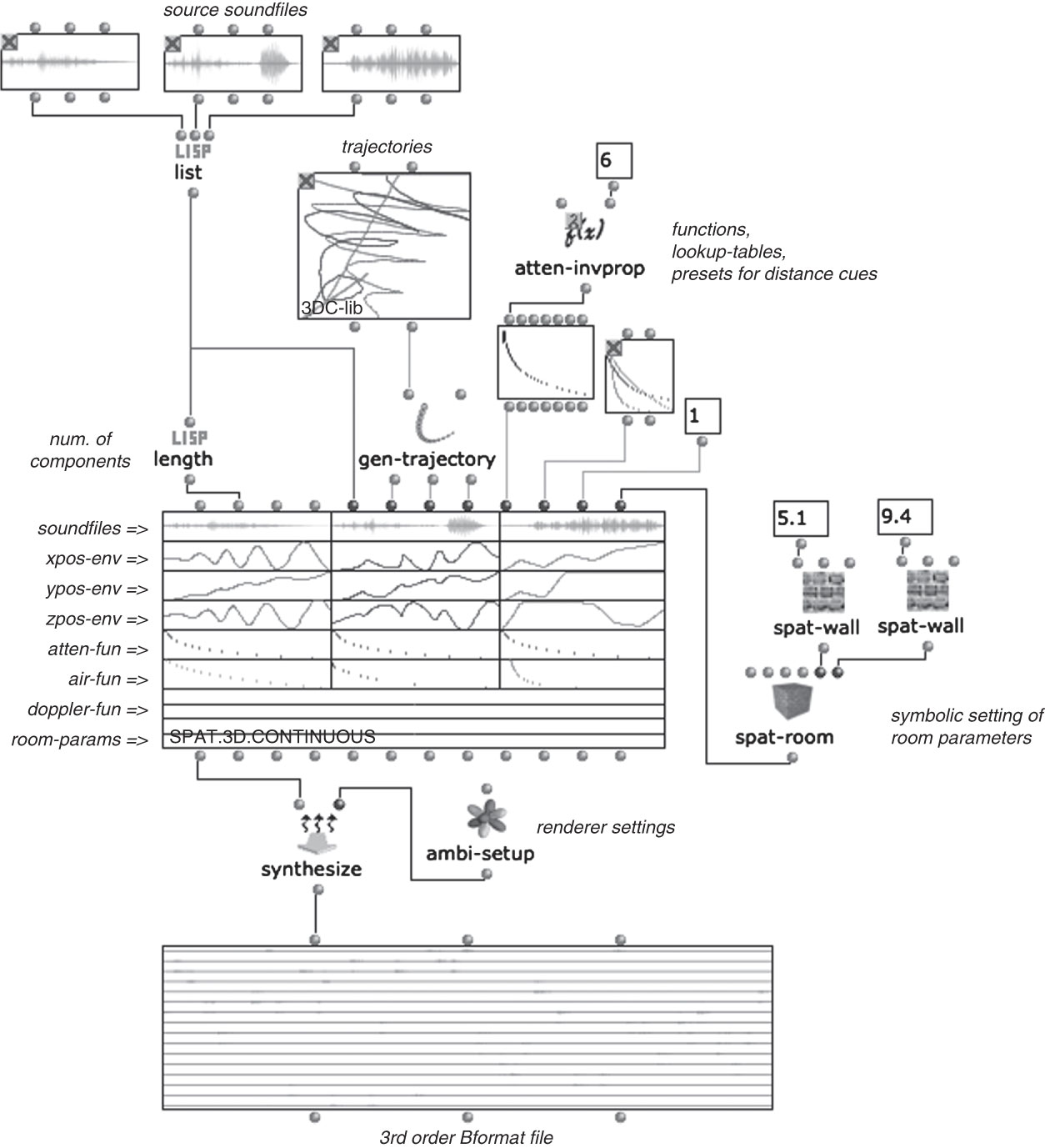
Rather than hard-wiring the equations for rendering of perceptual cues into the spatialisation engines directly, we implemented a table-lookup system for greater efficiency and flexibility. Lookup tables can be generated using pre-defined (see Section 4.2.2) or user-defined functions, and manually edited using OpenMusic’s graphical breakpoint-function editors. These tables can then be connected to the corresponding slot of a class to be applied to a specific sound source (see figure 4), or provided as global tables for the whole spatial sound rendering process.
Example for a sound spatialisation process using the OMPrisma class spat.3D.continuous. The gen-trajectory function converts a 3DC-lib object containing 3-dimensional trajectories into envelopes for x, y, z. Functions, pre-defined lookup-tables and presets are used to control the rendering of perceptual distance-cues. Room-characteristics are specified via the function spat-room. The function ambi-setup is used to set global parameters for the rendering process.
4.1.3. Room effects
Room acoustics and reverberation are important perceptual cues for the localisation of a sound source, and provide information on a surrounding environment’s size, shape and material (Blauert Reference Blauert1983). The description of room effects is conceptually different from the description of sound sources and therefore requires alternative control strategies. Depending on the underlying model and implementation of a reverberation algorithm the control interfaces can vary to a great extent (for example perceptual vs. physical models) and often require the setting of many individual parameters, which might clutter up the interface when specified as individual slots of a class. Thus, in OMPrisma room parameters are defined in tables, as a compact data structure (provided to a single slot of a class), which can be edited graphically or algorithmically directly in OM, and imported/exported as files to disk. Currently, two spatial sound rendering classes in OMPrisma include reverberation: RVBAP and SPAT. The reverberation algorithm in RVBAP is implemented as a feedback delay network based on digital waveguides, while SPAT implements a shoebox room-model based on recursive rendering of discrete reflections. Note that due to Csound’s dynamic instantiation paradigm the full range of parameters of the spatial sound rendering engine is available for each individual sound source. As with any other matrix slot, room parameters can be set globally for the whole rendering process or controlled individually for each component.
4.1.4. Within the loudspeaker array
The placement of virtual sound sources within the surrounding loudspeaker array is a feature often desired by composers, which is difficult or even impossible to realise with many spatial sound rendering techniques. A number of works have addressed this issue (Menzies Reference Menzies2002; Daniel Reference Daniel2003); however, these solutions are mostly idiosyncratic to a given spatial sound rendering concept and can be difficult to control for a non-expert user and without adequate technical equipment. In order to have a consistent approach for different spatial rendering classes we implemented the simple and popular technique of decreasing the directionality of a sound source as it enters the speaker array towards the listener, approaching complete monophony (i.e. all speakers contributing equally) at its centre. For classes implementing VBAP, for example, this is accomplished through implicit control of the ‘spread’ parameter (Pulkki Reference Pulkki1999); in the case of Ambisonics, via controlled decrease of gain coefficients for higher-order components (as described in Schacher and Kocher Reference Schacher and Kocher2006). This behaviour is optional and can be tweaked or bypassed if wished.
4.2. Control strategies
OMPrisma is designed to provide a higher-level abstraction layer for spatial sound scene description which is independent of the underlying rendering implementation. Accordingly, all classes share a structured interface which complies with current specifications of the Spatial Sound Description Interchange Format (SpatDIF, Peters et al. Reference Peters, Ferguson and McAdams2007). Control parameters (i.e. class slots) are organised into conceptual groups (or namespaces), such as soundfile-player parameters, position data, renderer-specific parameters (such as the ‘spread’ parameter for VBAP), source pre-processing settings and reverberation parameters. An overview of OMPrisma classes with respective slots is given in the Appendix. Figure 4 shows an example of a complete spatialisation process including conversion of a 3DC-lib into individual trajectories for position control, symbolic setting of room parameters and rendering of perceptual distance cues. Global settings for the rendering process are provided directly to the synthesize method, independently of the spatial sound scene description.
4.2.1. Trajectories
Trajectories for position-control of sound sources can be defined via geometric objects, such as breakpoint-functions (BPFs), 2D breakpoint-curves (BPCs), and 3D-curves (3DCs, see figure 1). The function gen-trajectory unfolds these geometric objects in time and returns the corresponding control data (envelopes for each Cartesian dimension) using two complementary strategies: in ‘constant speed’ mode, the sound source will travel along the trajectory with constant speed, while in ‘constant time’ mode it will respect a constant time interval between successive points in the trajectory. As an additional feature, the gen-trajectory function allows the generation of B-Spline curves; that is, polynomial interpolations between the object’s initial control points. This way, a trajectory can for example be specified manually with a few breakpoints, and its curvature controlled using this function. Obviously, trajectories can be set and modified via pre-defined or user-defined algorithms. Alternatively, a new object 3D-trajectory was implemented, which allows the assignment of time-tags to spatial points in the trajectory, either explicitly or automatically (deduced from surrounding points).
After the spatio-temporal morphology of a trajectory has been defined, its absolute playback speed can be controlled via frequency envelopes (individually for each Cartesian dimension). If no frequency envelopes are specified, the speed of a trajectory is implicitly scaled to fit the duration of its corresponding synthesis event (e.g. the duration of the soundfile). The use of frequency envelopes allows for dynamic control of the speed-of-travel of a sound source (including stopping or reversing the travel direction), creating spatial patterns (e.g. spirolaterals and lissajous figures), or working with audio-rate oscillations and frequency modulations at the border between sound synthesis and spatialisation. As with any matrix parameter, trajectories can be set globally or specified independently for each component (i.e. sound source).
4.2.2. Function library
OMPrisma features a ‘compositional toolbox’ of functions and utilities for generation and manipulation of spatialisation data. The function library includes tools for processing of 2D or 3D breakpoint-curves, such as interpolations in Cartesian or spherical coordinates, geometric transformations (e.g. rotations, scaling, mirroring), and stochastically driven manipulations such as perturbations and clusterings. For rendering of perceptual distance-cues a set of pre-defined functions are provided which implement commonly used equations to control the simulation of attenuation, air-absorption and Doppler shifts as functions of distance. Yet another category are renderer-specific functions, used for example to set reverberation/room parameters. The spat-room function shown in figure 4, for example, allows the setting of physical properties of a shoebox room-model in a symbolic way by connecting functions describing characteristics of individual walls (spat-wall) to a global room-model (spat-room). Finally, various utilities are provided, for example for configuration of loudspeaker setups, or to perform conversions between coordinate systems. Since these tools are embedded in a programming environment, they can be easily adapted, extended and related to the extensive set of libraries and features of OpenMusic.
4.2.3. Algorithmic sound scene manipulation
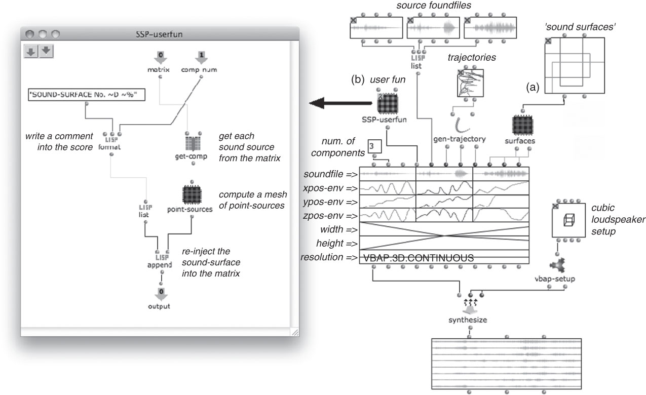
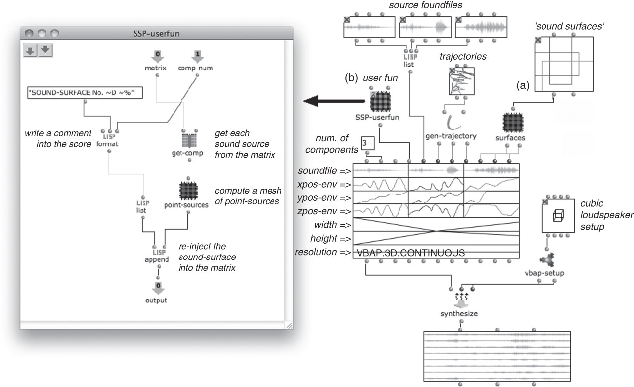
A particularly powerful concept inherited from the OMChroma synthesis system is the user-fun. This function, written directly in LISP or defined graphically in an OpenMusic patch, can access and modify the contents of a matrix and defines programs in order to manipulate, possibly generate or remove elements before starting the rendering process. User-funs can take additional arguments (provided as inlets to the matrix), which allows the user to introduce new control-parameters in the spatialisation process. This paradigm constitutes a powerful tool for selective and global manipulations of the matrix data, such as groupings, rotations/translations of sound source positions, or arbitrary rule-based transformations of entire spatial sound scenes. One possible application is the modelling of composite sound sources emitting sound over an extended space by breaking the original sound source up into a set of independent point sources. Figure 5 shows a graphically defined user-fun implementing the concept of Sound Surface Panning (as described in Ramakrishnan et al. Reference Ramakrishnan, Goßmann and Brümmer2006): for each sound source in the matrix a two-dimensional shape is specified, which is synthesised as a mesh of evenly distributed point sources. This process is controlled using the same data as in figure 4 (i.e. soundfiles, trajectories) and rendered into a multichannel soundfile using VBAP. Note that, thanks to the common control-interface for OMPrisma classes, the same user-fun and global processing can be applied to any other spatial sound rendering class. Similarly, we have employed the user-fun to implement W-panning (described in Schumacher and Bresson Reference Schumacher and Bresson2010).
Implementation of Sound Surface Panning via a user-fun applied to an OMPrisma matrix. a) Sound surfaces are graphically defined via BPC objects and provided as additional parameters (width/height/resolution) to the matrix. The patch labelled ‘SSP-userfun’ (b) is set as user-fun for the matrix, and therefore evaluated for each component in order to replace the sound sources with ‘sound surfaces’.
4.3. Decoding and diffusion: the Multiplayer
For any spatial sound composition tool it is of great importance that the user be able to listen to the results immediately. A tight auditory feedback loop between composition and reproduction facilitates efficient workflow and allows tweaking and fine-tuning the spatialisation processes via perceptual evaluations. Another important aspect is the ability to adjust the reproduction in real-time in order to adapt to a given environment, such as a specific studio setup or concert venue. This might include tasks such as the routing of logical output channels to physical devices, the adjustment of gains or time-delays for specific channels, or in the case of encoded formats setting and tweaking decoder parameters in real-time.
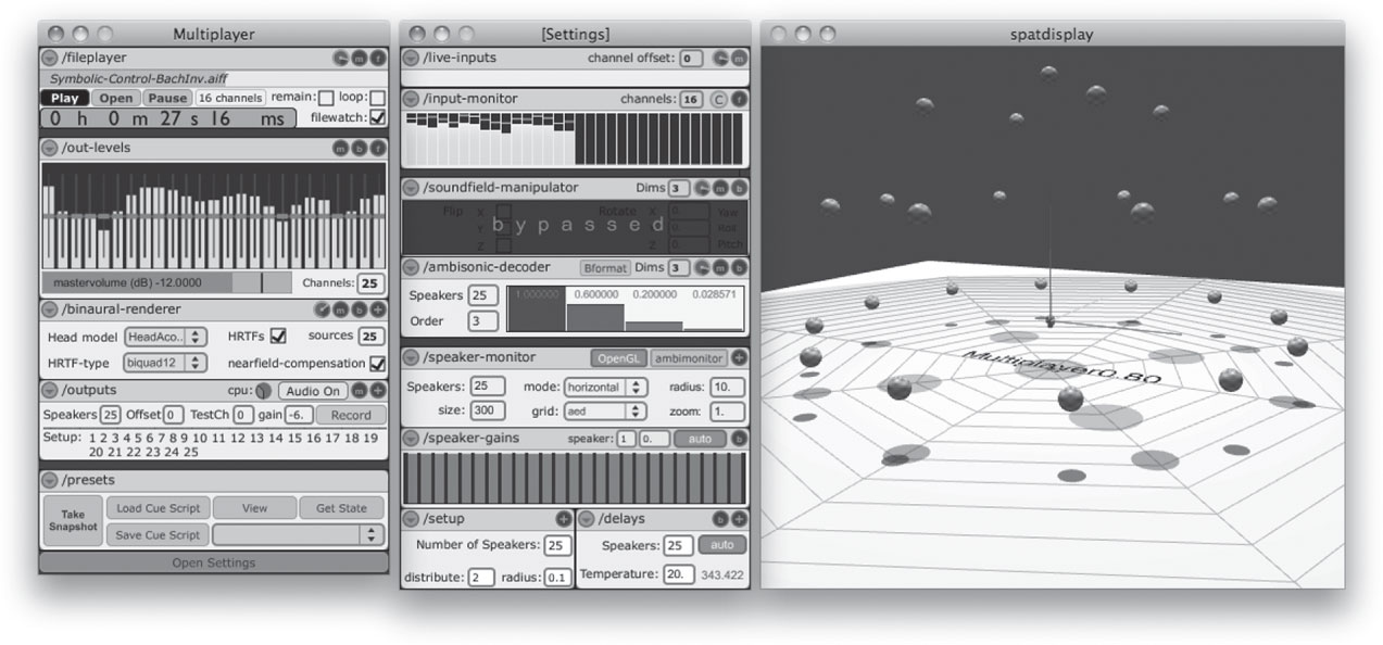
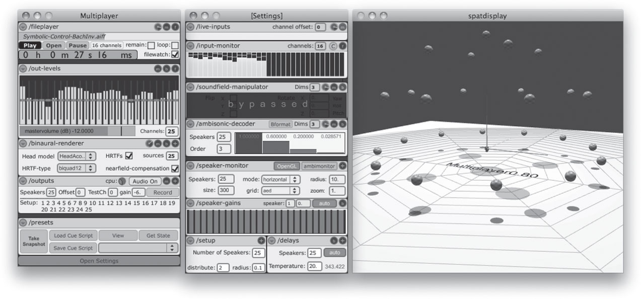
The Multiplayer is a standalone application for decoding and diffusion of interleaved multichannel soundfiles in different formats. It is implemented as a set of modules complying with the Jamoma framework for Max/MSP (Place and Lossius Reference Place and Lossius2006). It is intended to facilitate the work on spatial sound compositions in changing environments and for different loudspeaker setups, without requiring any expert-knowledge from the user. Figure 6 shows a screenshot of the Multiplayer application.
The Multiplayer standalone application decoding a third-order Bformat soundfile. On the right-hand side is a 3D visualisation of a hemispherical loudspeaker setup.
4.3.1. Integration
The Multiplayer seamlessly integrates into the workflow with OMPrisma via bidirectional communication using Open Sound Control (OSC) (Wright Reference Wright2005). Once the communication has been established, the Multiplayer can safely be sent to the background and entirely controlled from OM (using the same transport controls as OM’s internal players). Optionally, the Multiplayer can be synchronised with rendering settings in OMPrisma, in the sense that it will automatically update its configuration accordingly; in other words, no switching between applications is required.
4.3.2. Adaptability
Other important aspects for a decoding or diffusion application are compatibility with different formats and adaptability to different reproduction environments. The Multiplayer dynamically re-builds its internal dsp-structure via scripting (i.e. adds or removes channels) to match a given reproduction situation. Modules are provided for sound field manipulations (rotations and mirroring along the principal axes), Ambisonics decoding, numerical and graphical interfaces for configuration of loudspeaker setups, and binaural rendering. Sound pressure and time-differences in non-equidistant loudspeaker setups can be either automatically compensated (via loudspeaker positions) or manually balanced.
4.3.3. Auralisation
Composers are often required to elaborate musical works using loudspeaker configurations which are different from the intended reproduction setup in the performance venue. To address this issue, the Multiplayer provides a binaural rendering module for virtual loudspeaker binauralisation; that is, simulating a certain loudspeaker setup by treating the loudspeakers as virtual sound sources. Another benefit of this feature is the possibility of auditioning spatial sound scenes for various loudspeaker configurations (e.g. experimenting with irregular setups) and from different listening positions. It also allows the work with OMPrisma in the complete absence of loudspeakers. Moreover, it can be employed for rendering of binaural mixdowns. Note that all parameters are accessible via OSC, allowing the use of head-tracking devices for interactive control of the binaural rendering.
5. From Sound Source Spatialisation to Spatial Sound Synthesis
The process of sound spatialisation can be carried out on multiple time-scales (Roads Reference Roads2001). While traditional diffusion practices are usually limited to spatial movements that can be performed in real-time, there is no such restriction using digital signal processing techniques. Much as the development of analogue studio techniques (and, later, the digital synthesiser) made it possible to manipulate sound below the level of individual sound objects in the domain of sound synthesis, spatialisation processes can be applied to the microstructure of a sound in order to synthesise sounds with complex spatial morphologies.
5.1. Spatial sound synthesis
Within the presented framework we consider the term spatial sound synthesis most appropriate to denote the extension of sound synthesis algorithms into the spatial domain, i.e. as a general term to express spatialisation processes at the micro-level of sound. Several systems have been described which allow for spatial sound synthesis applications: Torchia and Lippe (Reference Torchia and Lippe2004) presented a system for real-time control of spectral-diffusion effects which allows the user to filter a sound into its spectral components and spatialise them individually. Scatter (McLeran, Roads, Sturm and Shynk 2008) is another original system for granular synthesis, which allows spatial positioning of individual grains using dictionary-based methods. The Spatial Swarm Granulator (Wilson Reference Wilson2008) allows the control of spatial positions of individual grains based on Reynold’s Boids algorithm (Reynolds Reference Reynolds1987). Kim-Boyle (Reference Kim-Boyle2008) gives an overview of frequency-domain spatial distributions, mostly controlled via particle and agent systems. Interestingly, the author stresses the need for ‘an interface with the power to control and transform coordinates for hundreds of particles which at the same time does not overwhelm the user with massive banks of control data’. In their presentation of Spatio-Operational Spectral Synthesis (which is conceptually close to our notion of spatial sound synthesis), Topper et al. (Reference Topper, Burtner and Serafin2002) describe the process as ‘taking an existing synthesis algorithm and breaking it apart into logical components’ and then ‘[assembling] the components by applying spatialisation algorithms’.
The OMChroma system, which builds upon an initial implicit decomposition of the sound synthesis process into ‘components’ (see Section 3.2), lends itself particularly well to this idea of spatial sound synthesis. The separation into logical components is given in the initial design of the OMChroma classes and generalised by the use and control of matrix structures. The same paradigm is adopted for the individual spatialisation of each synthesis component.
5.2. Implementation with OMChroma/OMPrisma
Generalised spatial sound synthesis processes can be achieved in OMChroma/OMPrisma by designing Csound instruments to perform both sound synthesis and spatial sound rendering. However, given the number of possible combinations of existing synthesis classes (in OMChroma) and spatialisation classes (in OMPrisma), the explicit implementation of individual spatial sound synthesis instruments would lead to an excessive amount of classes. A more sensible solution is to combine sound synthesis instruments with spatial renderers dynamically, in order to create compound instruments capable of spatial sound synthesis. In terms of signal-flow this idea can be described as an automatic detection and redirection of the output of the synthesiser to the input of the spatial sound renderer (that is, replacing the former input sound source). This is a non-trivial task, however, which is carried out in two steps:
1. A new Csound instrument is created by merging the original synthesis and spatial rendering instruments. In the synthesis instrument, the variable bound to the signal output must be identified, while, on the spatial rendering side, the original input and its internal dependencies must be detected and replaced by the synthesis output. Variable declarations, bindings and redundancies must be handled between both instrument-parsing processes. Useless parameters must be omitted (e.g. the ‘soundfile-player’ part in the spatialisation instruments), and the Csound p-fields order and indexing must be adapted accordingly.
2. The merged Csound instrument code is then used to create a new hybrid class starting from the two inital ones (synthesis and spatial rendering). Fortunately, Common Lisp and CLOS provide powerful tools for meta-object programming and dynamic class definition (Gabriel et al. Reference Gabriel, White and Bobrow1991). After inspecting the different slots and properties of the respective classes, a new one is defined by keeping the common fields (e.g. e-dels, durs) and combining the specific ones of the different instruments. The instantiation of the resulting class is done using the corresponding slot values in the two initial objects.
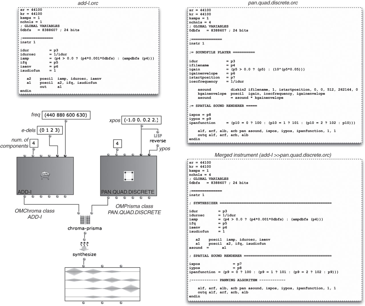
From a user’s perspective this merging-process is accomplished by simply connecting two objects (any synthesis class from OMChroma and any spatial rendering class from OMPrisma) to the function chroma-prisma, which internally creates the new merged-orchestra class and outputs an initialised instance. This resulting instance can eventually be plugged into the synthesize function in order to perform the spatial sound synthesis. This process is illustrated in figure 7, in which an additive synthesis class is merged with a quadrophonic spatial sound rendering class.
Spatial sound synthesis: merging synthesis and spatialisation classes in OMChroma. At the bottom right is the merged Csound instrument generated automatically from the class add–1 (add–1.orc, top left) and the class pan.quad.discrete from figure 2 (pan.quad.discrete.orc, top right).

This system therefore constitutes a powerful synthesis framework, enabling high-level control over the full range of sound synthesis and spatialisation parameters for each individual component – partials, grains, or any other primitive components of a given synthesis algorithm.
6. Example Applications
One of the main interests of the OMPrisma framework is its integration into a general compositional environment (OpenMusic). This embedding leads to novel possibilities for integrating symbolic, sound and spatialisation data into compositional frameworks and offers a degree of control difficult to achieve using conventional tools. In this section we show a number of examples of how spatial parameters can be related to other musical dimensions within a compositional framework.
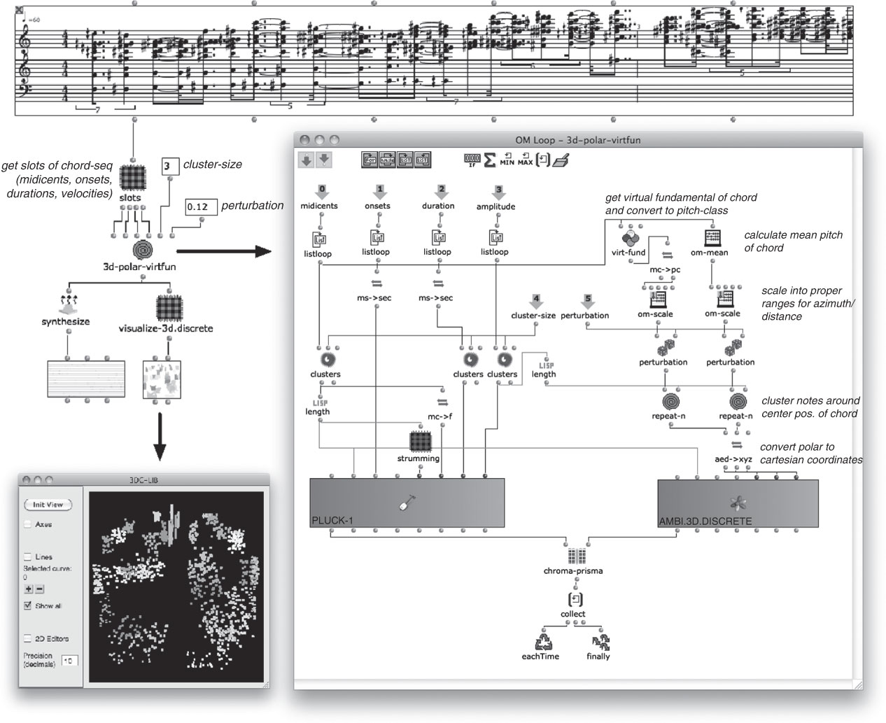
In figure 8, symbolic musical material (a score in common music notation) is used as input data to control both sound synthesis and spatialisation parameters. The spatial positions for the synthesised sound components (plucked-string synthesis) are derived via arithmetic operations from the chords/notes contained in the score: for every chord the ‘virtual fundamental’ is calculated; that is, the highest fundamental frequency for which the notes of the chord could be thought of as harmonic partials. This fundamental frequency is first converted into a pitch-class value and then rescaled and interpreted as azimuth angle (i.e. a position on a horizontal circle). Similarly, the mean-pitch of the same chord is used to calculate an elevation angle. With these two polar coordinates a position for each chord on the surface of a unit-sphere is determined. The positions of the individual notes of each chord are specified via controlled perturbations of its centre position. The resulting ‘spatial clusters’ (each corresponding to a chord) are visualised in the 3DC-lib at the bottom left of the figure.
Symbolic control of a spatial sound synthesis process in OpenMusic. The visual program on the right hand side (3d-polar-virtfun) converts the symbolic musical materials to synthesis and spatialisation parameters. The spatial positions of the synthesised score materials are shown in the 3DC-lib at the bottom left.
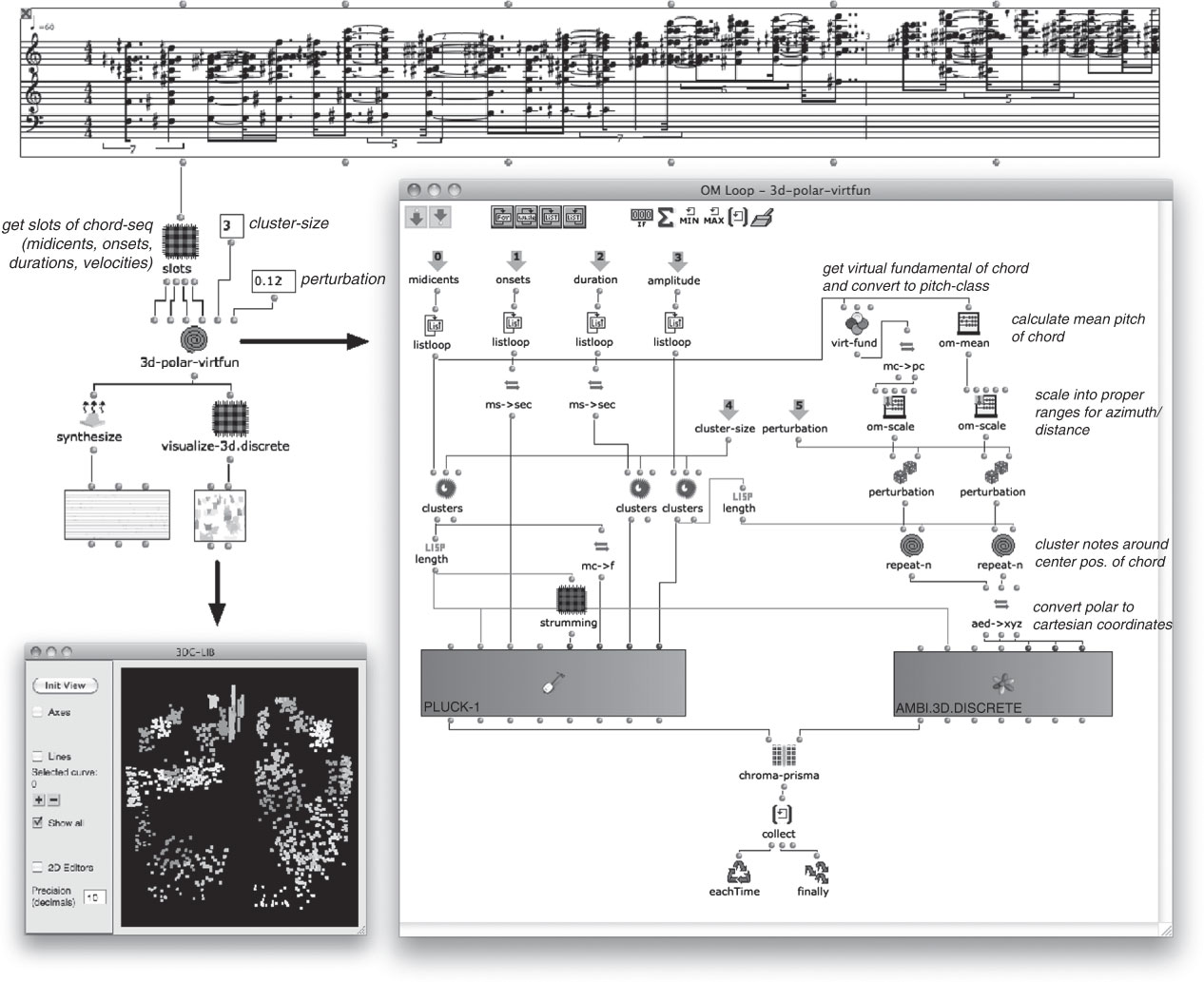
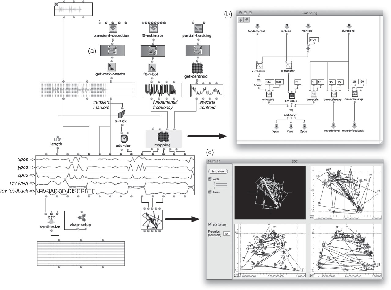
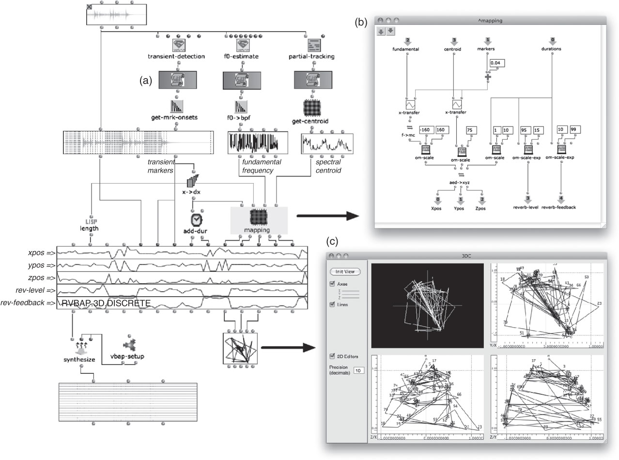
Figure 9 shows a somewhat complementary approach: the use of concrete, external data to control the spatialisation of an existing soundfile.Footnote 4 In this example, the spatialisation parameters of a percussion (tabla) solo are controlled exclusively via data which is extracted from the soundfile itself using OpenMusic’s sound analysis tools (Bresson Reference Bresson2006). First, the source soundfile is analysed for transients in order to segment the percussion solo into individual tabla strokes. A fundamental-frequency estimation and partial-tracking is performed, from which profiles for pitch and spectral centroid are generated (a). For every soundfile, its fundamental frequency and spectral centroid value is looked up and mapped to azimuth and elevation angle for spatialisation control. Since we are working in a differed-time paradigm, the duration of each segment can be used as control data to determine its distance from the centre position, and to set reverberation parameters (b). Consequently, every tabla stroke in the original soundfile will be assigned an individual spatial position and reverberation characteristics, determined by its pitch, spectral centroid and duration.
Interfacing sound spatialisation and analysis tools in OpenMusic. Control data is derived from sound analyses (transient detection, fundamental-frequency estimation and partial-tracking) of the original soundfile (a). A visual program (mapping) specifies mapping-functions to determine spatial positions and reverberation characteristics (b). The 3DC visualises the spatial distribution of the sound segments; indices denote their order of succession (c).
A large variety of spatial sound synthesis applications can be realised by freely combining sound synthesis and spatialisation instruments. Granular synthesis, for instance, is a popular model for time-domain spatial sound synthesis (see for example McLeran et al. Reference McLeran, Roads, Sturm and Shynk2008; Wilson Reference Wilson2008). Typically, each sound grain is assigned an individual position in space, often controlled stochastically (rather than literally) in order to reduce the large number of parameters to a few manageable variables.
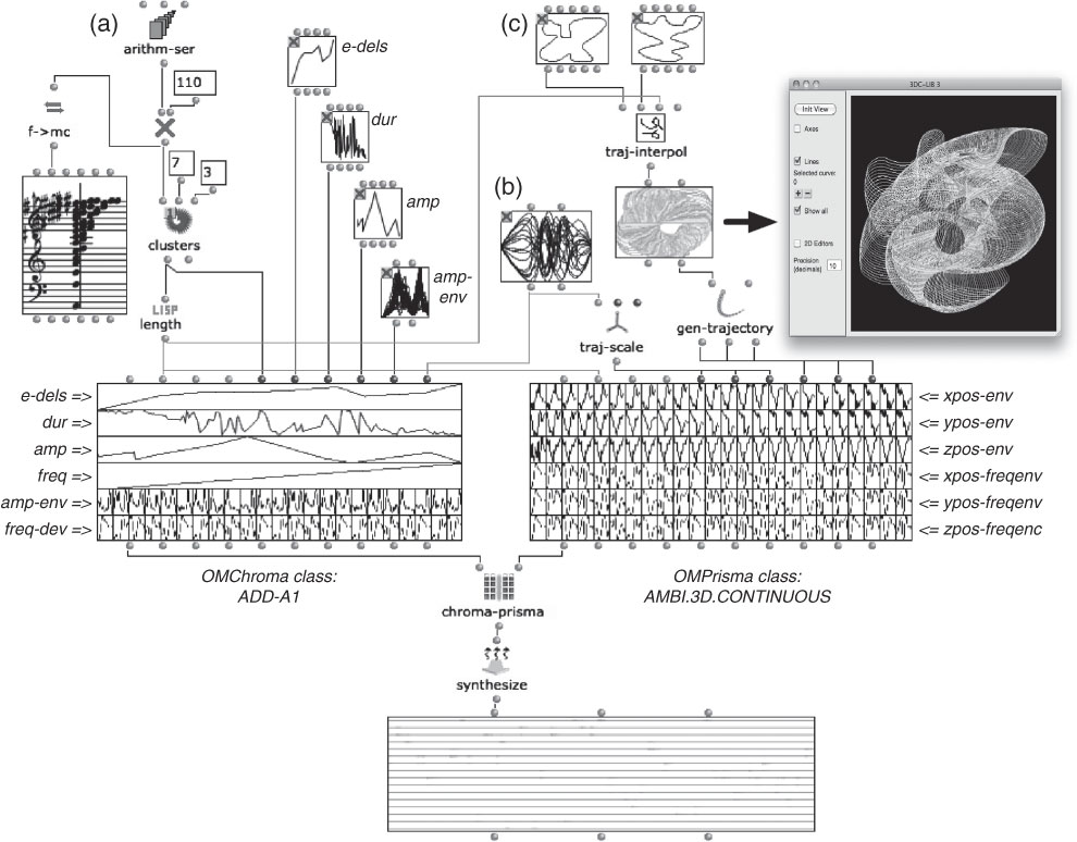
Another interesting model is ‘spatial additive synthesis’: in spatial additive synthesis a complex sound is synthesised from elementary sinusoidal components which are spatialised individually. Figure 10 shows an example for continuous control of spatial additive synthesis in which hundreds of partials are synthesised, each with its individual set of dynamically changing sound synthesis and spatialisation parameters. It is also a nice illustration of how a complex spatial sound synthesis process – requiring large amounts of control data – can be managed via a small number of conceptually meaningful, high-level abstractions.
Spatial additive synthesis using the classes add–1 and ambi.2D.continuous: (a) a harmonic spectrum is generated (visualised as a chord) and additional partials (micro-clusters) added around each harmonic; (b) a set of envelopes (BPF-lib) is used to control both sound synthesis and spatialisation parameters; (c) two manually defined (i.e. hand-drawn) trajectories are interpolated over the number of partials. Each partial is assigned an individual trajectory, displayed in the 3DC-lib on the right-hand side.

7. Conclusion
We have presented a system for the symbolic control of sound source spatialisation and spatial sound synthesis in compositional contexts. This system has been implemented as an extension of OMChroma in the OpenMusic computer-aided composition environment. Embedded in this framework, spatial sound scenes can be generated and manipulated via high-level structures and algorithms, which allows for explicit control of arbitrary numbers of control parameters, difficult to achieve via manual editing or other conventional approaches (e.g. real-time, track-based).
The visual programming and composition environment provides an extensive set of tools for the generation, manipulation and control of spatial parameters and processes. More importantly, the integration of spatialisation tools into environments for computer-aided composition allows spatialisation to be treated as a structural parameter, and enables complex relationships with other musical dimensions and in relation to a global compositional framework. Interesting relationships can for instance be created using external data derived from sound analyses or any other musical/extra-musical source or process.
OMPrisma separates the different stages of sound spatialisation into several layers as proposed in Peters et al. (Reference Peters, Lossius, Schacher, Baltazar, Bascou and Place2009), with authoring in OM programs, description in matrices, interpretation via the synthesize function, rendering via Csound orchestras, and, finally, the decoding and communication with physical devices using the external Multiplayer application.
Thanks to an original class-merging system between OMChroma (for sound synthesis) and OMPrisma (for spatial sound rendering), the concept of spatial sound synthesis is implemented in a generic way, allowing arbitrary combinations of sound synthesis and spatial sound rendering techniques. The control of sound spatialisation is tightly integrated in the compositional framework and benefits from the same flexibility and expressive power as sound synthesis and general compositional processes.
Future work is planned in several directions: The existing class-library could be extended with other spatial sound rendering concepts, such as SUG. More processor-demanding approaches such as ViMiC or WFS would be particularly promising candidates (facilitated by the offline-rendering paradigm). It would also be interesting to use the system in the context of directivity synthesis (Warusfel and Misdariis Reference Warusfel and Misdariis2001), for instance to synthesise artificial sounds with intricate directivity patterns. More complex processing chains could be envisaged in this framework, including for instance spectral diffusion or other spatial audio effects. On the ‘control’ level, different OpenMusic tools such as the maquette, for temporal modelling (see Agon Reference Agon1998), or the cr-model for abstract sound representations based on time–frequency structures (see Bresson, Stroppa and Agon Reference Bresson, Stroppa and Agon2007) form interesting contexts in which spatial sound control could be integrated.
So far OMPrisma has been used for the composition of a number of works, most notably Cognitive Consonance by C. Trapani, performed at the Ircam Agora Festival, Paris 2010. OMPrisma is distributed with the OpenMusic package through the IRCAM forum and is also available as an open source OM-library. More information and sound examples are available at www.music.mcgill.ca/~marlon/OMPrisma.