1 Introduction
When a stream of flow interacts with a fixed boundary, a vorticity is created in the boundary layer and discharged into fluid to form a self-organized pattern known as the von Kármán vortex street. Previous studies of this celebrated topic include its formation (Williamson Reference Williamson1996), Strouhal–Reynolds number relations (Fey, Konig & Eckelmann Reference Fey, Konig and Eckelmann1998; Williamson & Brown Reference Williamson and Brown1998; Roushan & Wu Reference Roushan and Wu2005), control (Choi, Jeon & Kim Reference Choi, Jeon and Kim2008), etc.
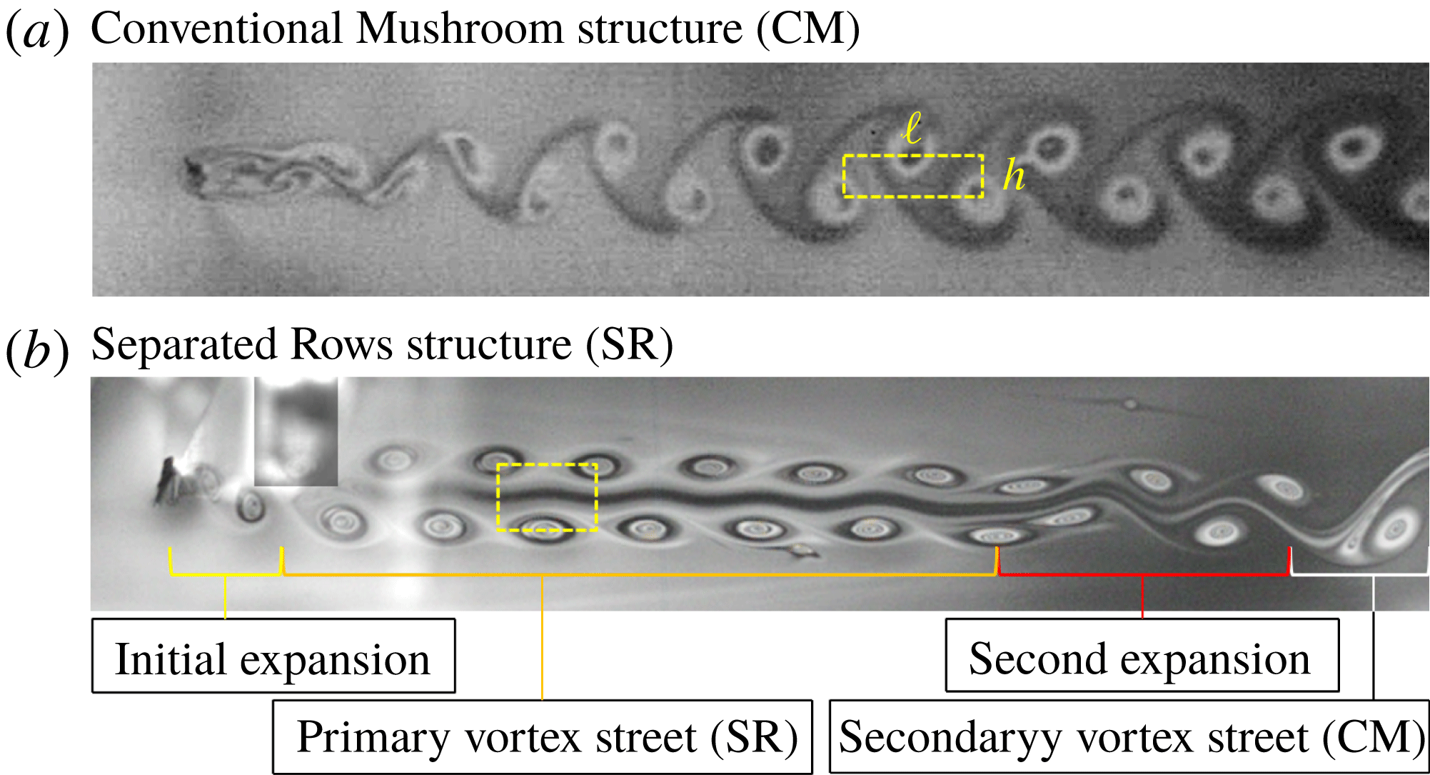
We report vortex streets whose spatial structure is different from that of commonly observed ones. In figure 1, two vortex streets are morphologically different as follows. First, the two rows of the vortices in figure 1(b) are separated by a thin layer of irrotational fluid while the vortices in figure 1(a) are intermingled. The structure in figure 1(b) resembles the Kelvin–Stuart cat’s eye flow, which is a quintessential feature of the shear layer instability. This observation indicates that there are two length scales in the problem, where one is the thickness of the boundary layers and the other is their separation distance. Second, the Kármán ratio is higher in figure 1(b) than in figure 1(a). The Kármán ratio
 $r_{K}$
is defined as the ratio between
 $h$
, the distance between two rows of vortices, and
 $\ell$
, the distance between two vortices in the same row, i.e.
 $r_{K}\equiv h/\ell$
, and has an implication regarding the stability of the vortex street. Using the point vortex model, von Kármán (Reference von Kármán1911) has shown that only a vortex arrangement having
 $r_{K}=\cosh ^{-1}(\sqrt{2})/\unicode[STIX]{x03C0}\approx 0.281$
is stable. His prediction of the narrow range of the stability is at odds with experiments that showed that vortex streets exist over a range
 $0.25<r_{K}<0.52$
(Goldstein Reference Goldstein1938), and Hooker (Reference Hooker1936) has shown that the action of the viscosity broadens the range of the stability.
Two wake structures in a flowing soap film. (a) The conventional mushroom structure is created using a circular object. The Kármán ratio,
 $r_{K}$
, is measured to be 0.27. (b) The separated rows structure is created using a triangular object (
 $r_{a}=0.5$
). This exotic structure is characterized by a thin layer of irrotational fluid between two vortex rows and a higher
 $r_{K}$
, which is measured to be 0.63 in this particular case. The bright spot on the left-hand side in (b) is a reflection from a part of the apparatus. The brightness and contrast of the image are modified to show the detail of the flow structure. The Reynolds number is the same (
 $Re\approx 660$
) in both cases.

A wake structure similar to that in figure 1(b) has been perceived as a precursor to the breakdown of a primary vortex street in two-dimensional flows (Inoue & Yamazaki Reference Inoue and Yamazaki1999; Vorobieff, Georgiev & Ingber Reference Vorobieff, Georgiev and Ingber2002; Wang et al. Reference Wang, Tian, Jia, Lu and Yin2010; Kumar & Mittal Reference Kumar and Mittal2012; Dynnikova, Dynnikov & Guvernyuk Reference Dynnikova, Dynnikov and Guvernyuk2016) and three-dimensional flows (Cimbala, Nagib & Roshko Reference Cimbala, Nagib and Roshko1988), but we find that this is not always the case. It had been considered as an interim structure that occurs only when the primary vortex street, which is an archetypal structure in figure 1(a), breaks down and is transformed to the secondary vortex street, which is also an archetypal structure. However, we find that this exotic structure also occurs in the primary wake without the presence of the archetypal structure when we use triangular objects to generate vortex streets. This observation indicates that the spatial structure in figure 1(b) is neither a far-field phenomenon nor a component of the wake transformation. For clarity of the ensuing discussions, we name the archetypal structure in figure 1(a) as the conventional mushroom structure (CM) and that in figure 1(b) as the separated rows structure (SR).
In this paper, we investigate the role of the boundary layer in the formation and structure of vortex streets. Previous observations of vortex streets indicate that the spatial structure depends on the initial condition that produces the vorticity (Kim & Wu Reference Kim and Wu2015). However, such an effect has not been studied in a systematic manner because the circular cylinder, which is used in most experiments in this area, has only a single length scale (the diameter) that determines the downstream flow structure. The current study uses bluff bodies with a triangular cross-section, and the height
 $H$
and the base
 $D$
of the triangle are independently varied. By using a triangular object of various aspect ratios
 $r_{a}=H/D$
, we independently vary the thickness
 $\unicode[STIX]{x1D6FF}$
of the boundary layers and the separation distance
 $D$
between two layers. This setting allows us to create various vortex structures and to manipulate the transition between them.
We find that there is a critical ratio between
 $\unicode[STIX]{x1D6FF}$
and
 $D$
that determines the stability of vortex streets. When
 $\unicode[STIX]{x1D6FF}/D>0.4$
, the vortex street is created in CM and is stable over the range of our experiments. When
 $\unicode[STIX]{x1D6FF}/D<0.4$
, the vortex street is created either in CM or in SR, and the vortex street is unstable and decays downstream. If the vortex street was created in CM, it gradually broadens to transform to SR. If the vortex street was created in SR, or has transformed to SR, it transforms back to CM through a sudden and full-scale rearrangement of vortices, as previously known as the secondary instability (Taneda Reference Taneda1959; Cimbala et al.
Reference Cimbala, Nagib and Roshko1988; Williamson & Prasad Reference Williamson and Prasad1993; Inoue & Yamazaki Reference Inoue and Yamazaki1999; Vorobieff et al.
Reference Vorobieff, Georgiev and Ingber2002; Wang et al.
Reference Wang, Tian, Jia, Lu and Yin2010; Kumar & Mittal Reference Kumar and Mittal2012; Dynnikova et al.
Reference Dynnikova, Dynnikov and Guvernyuk2016).
It is inferred from our results that the stability of vortex streets is determined by two mechanisms. In CM, the vortex street decays because the vorticity is dissipated through mixing of two rows. In SR, however, such dissipation through mixing does not happen, but the vortex street decays because of its unstable spatial arrangement. These two mechanisms act interchangeably, and an alternating sequence of CM and SR may be observed in a long channel.
2 Experimental set-up
The experiments are carried out in an inclined soap film channel (Georgiev & Vorobieff Reference Georgiev and Vorobieff2002; Kim & Wu Reference Kim and Wu2015). Our channel is approximately 2 m long and 5 cm wide, and we use a soap solution made of 2 % commercial dish soap (P&G Dawn), 5 % glycerol and remainder distilled water. The kinematic viscosity of the solution is
 $\unicode[STIX]{x1D708}=0.013\pm 0.001~\text{cm}^{2}~\text{s}^{-1}$
, measured by a Cannon viscometer. The flow speed and the thickness of the channel can be adjusted by the flow rate. Throughout the study, we fix the flow rate at
 $0.09~\text{cm}^{3}~\text{s}^{-1}$
. Under this condition, the flow speed
 $U$
is
 $60\pm 3~\text{cm}~\text{s}^{-1}$
and the thickness of the film is approximately
 $3~\unicode[STIX]{x03BC}\text{m}$
. The film is only slightly compressible because the flow speed is only 16 % of the Marangoni wave speed (Kim & Mandre Reference Kim and Mandre2017), indicating that the fluid medium is quasi two-dimensional.
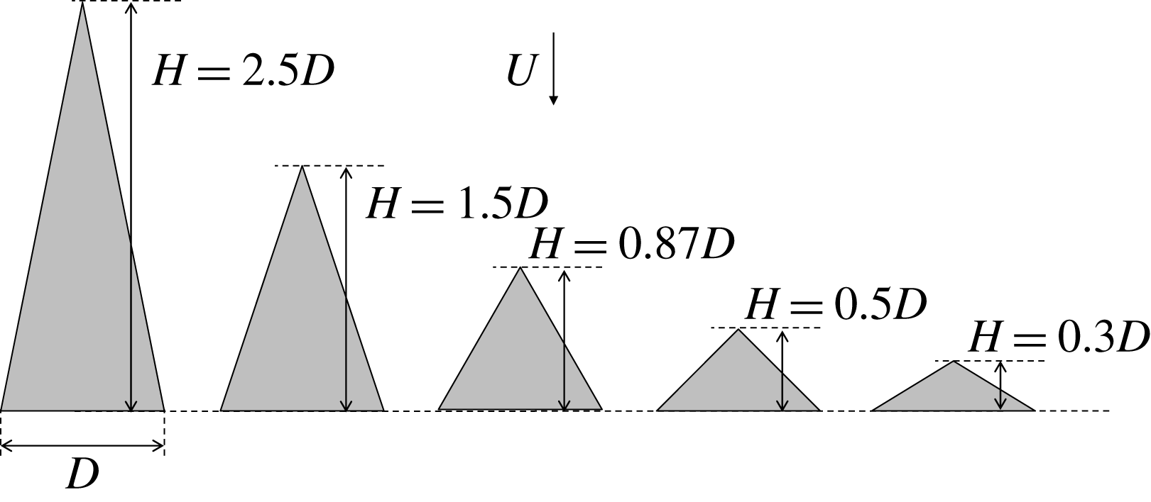
We generate vortex streets by inserting tapered rods into the soap film. Each rod has a triangular cross-section set at five different aspect ratios
 $r_{a}\equiv H/D=0.3$
, 0.5, 0.87, 1.5 and 2.5, where
 $H$
is the height and
 $D$
is the base of the triangle, as depicted in figure 2. The apex of the triangle faces the flow. The rods are made of titanium or aluminium, and each rod is carefully tapered to maintain a unique
 $r_{a}$
to the tip size
 $50~\unicode[STIX]{x03BC}\text{m}$
. Therefore, depending on the insertion depth of a rod to the soap film,
 $D$
varies from 0.5 cm to
 $50~\unicode[STIX]{x03BC}\text{m}$
. We define the Reynolds number using the base of the triangle, i.e.
 $Re\equiv UD/\unicode[STIX]{x1D708}$
. Since
 $U$
and
 $\unicode[STIX]{x1D708}$
are fixed in our setup,
 $Re$
is determined solely by
 $D$
.
Using these rods of various aspect ratios, we investigate the effect of the thickness of the boundary layer
 $\unicode[STIX]{x1D6FF}$
on the structure and the stability of vortex streets. The boundary layer is thicker when the aspect ratio of the rod is higher because the flow passes by a longer distance. We use the empirical relation
 $$\begin{eqnarray}\unicode[STIX]{x1D6FF}\simeq 6(r_{a}^{2}+0.25)^{1/4}Re^{-1/2}D,\end{eqnarray}$$
whose derivation is presented in appendix A.
Cross-sections of tapered rods used in the experiments. These rods are characterized by the aspect ratio
 $r_{a}=H/D$
, where
 $H$
and
 $D$
are the height the base. Vortex streets are generated by inserting a tapered rod to the soap film, as the apex of the triangle faces the flow.

Two video cameras are used for our measurements. A normal-speed camera (30 frames per second) is attached to a long-range microscope to monitor the insertion depth of the rods into the soap film, and
 $D$
is precisely determined. The vortex streets in the soap film are illuminated by a monochromatic light (low-pressure sodium lamp), and the interferogram is captured by a high-speed camera (Phantom V5, Vision Research) at up to 1900 frames per second. The visualization technique allows us to directly measure the flow structure. The field of view is approximately
 $8~\text{cm}\times 8~\text{cm}$
. It is wide enough to cover
 $40D$
–
 $100D$
depending on
 $Re$
, and the flow structures are monitored far downstream.
3 Results and discussion
3.1 Wake structures
The wake structure is clearly characterized by
 $\ell$
and
 $r_{K}$
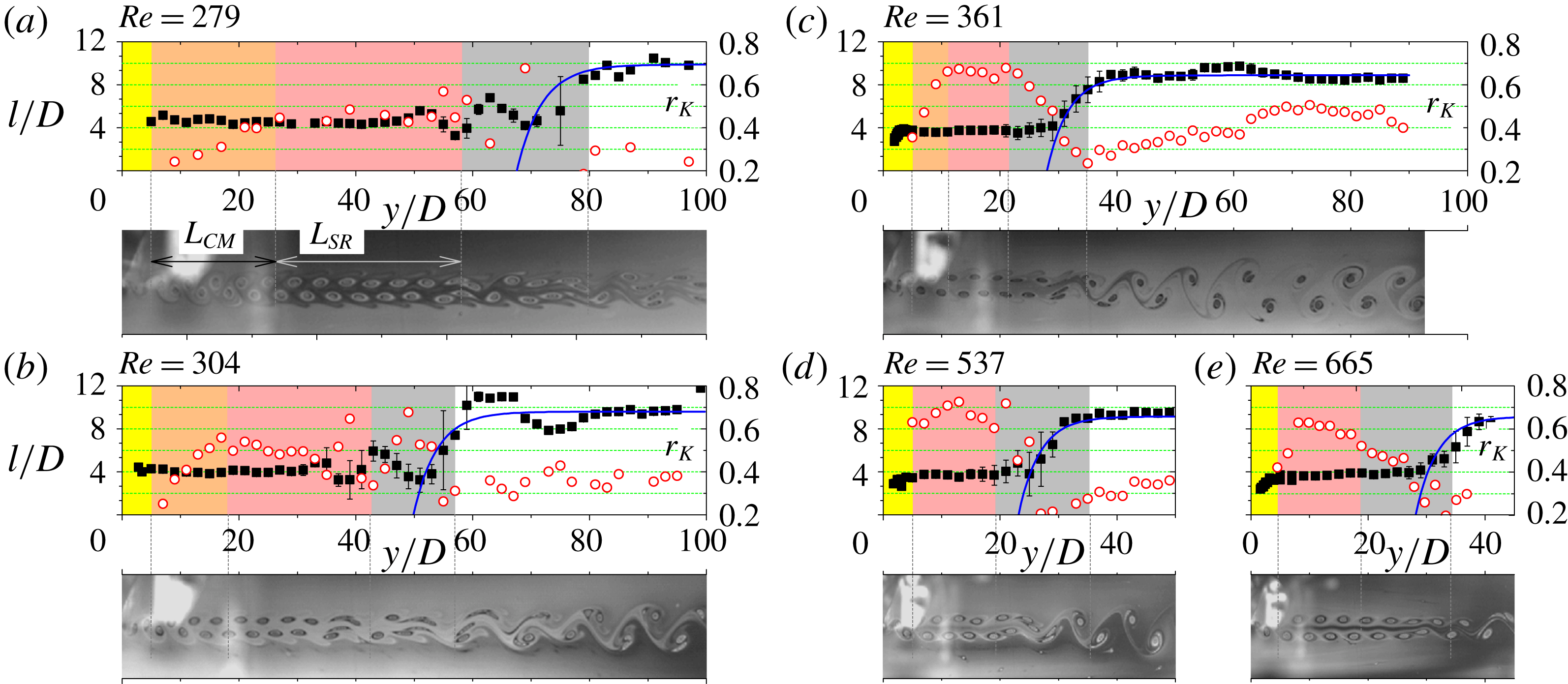
, the distance between two vortices in the same row and the Kármán ratio, respectively. In figure 3, we present our measurements of
 $\ell$
and
 $r_{K}$
for vortex streets generated by using the rod of
 $r_{a}=0.5$
, at
 $Re=279$
, 304, 361, 537, and 665 (
 $D=0.047$
, 0.053, 0.062, 0.095 and 0.127 cm). The measurements are plotted with respect to the downstream distance
 $y$
and normalized by the size of the rod
 $D$
. We find that a vortex street is separated into the following zones: (i) the initial expansion zone, (ii) the primary wake zone, (iii) the second expansion zone and (iv) the secondary wake zone.
The characterization of vortex structures. The longitudinal spacing between vortices
 $\ell /D$
(filled squares) and the Kármán ratio
 $r_{K}$
(open circles) are measured with respect to the downstream distance
 $y/D$
for vortex streets behind the tapered triangular rod of
 $r_{a}=0.5$
. A vortex street is separated into the following zones: (i) the expansion zone (shaded yellow), (ii) primary wake in CM (shaded orange) or in SR (shaded pink), (iii) the second expansion zone (SR
 $\rightarrow$
CM transition zone, shaded grey) and (iv) the secondary wake zone. We see that
 $\ell$
rapidly increases in the expansion zones and is stable and unchanged in the wake zones. The expansion is characterized as (3.5), as indicated by blue solid lines. Unlike
 $\ell$
, Kármán ratio
 $r_{K}$
is gradually increasing when the vortex street is in CM. The photographic images are rescaled by each respective
 $D$
and aligned with the horizontal axes of the plots.

In the initial expansion zone, the vorticity created in the boundary layer is discharged into the fluid and organized into the primary vortex street. In figure 3, this region is shaded yellow. The initial development of the spatial pattern has been discussed by Kim & Wu (Reference Kim and Wu2015). They have shown that the initial expansion is characterized by the exponential function
 $\ell =\ell _{1}[1-\exp (-y/y_{1})]$
, where
 $\ell _{1}$
is an asymptotic value and
 $y_{1}\sim D$
is a relaxation length . Our experiments show a similar trend in the initial expansion, and the extent of the initial expansion zone is less than
 $5D$
from the rod.
In the primary wake zone, the vortex street is either in CM followed by SR as displayed in figure 3(a–c) or entirely in SR as in figure 3(d,e). The CM part is shaded in orange and the SR part is shaded in pink. For the primary wake,
 $\ell$
is stable and does not change across
 $y$
, regardless of the wake structure. Our measurement shows that
 $\ell =\ell _{1}\approx 4D$
, and this is consistent with a previous report that used circular and square rods (Roushan & Wu Reference Roushan and Wu2005; Kim & Wu Reference Kim and Wu2015). Unlike
 $\ell$
,
 $r_{K}$
depends on the wake structure. When the vortex street is in CM,
 $r_{K}$
gradually increases with
 $y$
due to a subtle rearrangement of vortices that causes the vortex street to broaden. The rate of the broadening increases as
 $Re$
increases, and the broadening continues until the wake structure is transformed to SR. When the vortex street is SR, for the scenarios of either figure 3(a–c) or figure 3(d,e), both
 $h$
and
 $\ell$
do not depend on
 $y$
. We find that
 $r_{K}$
of SR ranges from 0.45 to 0.8 depending on
 $Re$
and
 $r_{a}$
. This range of
 $r_{K}$
is substantially higher than the theoretical prediction of the point vortex model
 $r_{K}=\cosh ^{-1}(\sqrt{2})/\unicode[STIX]{x03C0}\approx 0.281$
. These SR vortex streets with high
 $r_{K}$
are unstable and break down downstream, followed by a violent rearrangement of vortices in the secondary expansion zone.
The broadening of the vortex street in CM is caused by the erosion of vorticity through the mixing of two vortex rows. Birkhoff (Reference Birkhoff1953) has shown that in any plane flow satisfying the Navier–Stokes equation, the moment of the vorticity is constant, which implies the conservation of
 $h\unicode[STIX]{x1D705}$
, where
 $\unicode[STIX]{x1D705}$
is the vorticity of each vortex. In the primary wake zone of our experiments, two vortex rows of CM are close enough to get mixed. Therefore, the strength of vortices
 $\unicode[STIX]{x1D705}$
diminishes, which causes
 $h$
to increase. Whereas when the vortex street is in SR, the two vortex rows are well separated by the thin layer of irrotational fluid. In this case,
 $\unicode[STIX]{x1D705}$
remains unchanged, and the broadening does not take place.
We calculate the broadening of the vortex street by using a simple model. The linear model below assumes that the decay rate of
 $\unicode[STIX]{x1D705}$
is proportional to
 $\unicode[STIX]{x1D6FF}/h$
:
 $$\begin{eqnarray}U\frac{\text{d}\unicode[STIX]{x1D705}}{\text{d}y}=-\frac{\unicode[STIX]{x1D705}\unicode[STIX]{x1D6FF}}{h\unicode[STIX]{x1D70F}},\end{eqnarray}$$
where
 $\unicode[STIX]{x1D70F}$
is a time scale of the fluid medium that is supposedly independent of
 $\unicode[STIX]{x1D705}$
and
 $D$
. Using the conservation law
 $h\unicode[STIX]{x1D705}=h_{0}\unicode[STIX]{x1D705}_{0}$
, where
 $h_{0}$
and
 $\unicode[STIX]{x1D705}_{0}$
are values at
 $y=y_{0}$
where the primary wake zone begins, the solution of the model indicates that
 $h$
linearly increases with
 $y$
. The Kármán ratio is then derived as
 $$\begin{eqnarray}r_{K}=r_{K}(y_{0})+\frac{(y-y_{0})}{D}\frac{\unicode[STIX]{x1D6FF}}{U\unicode[STIX]{x1D70F}(\ell /D)}.\end{eqnarray}$$
Considering that
 $\unicode[STIX]{x1D6FF}\propto D^{1/2}$
and
 $\ell \propto D$
, we infer from (3.2) that the rate of broadening increases with
 $Re$
as observed in the experiments.
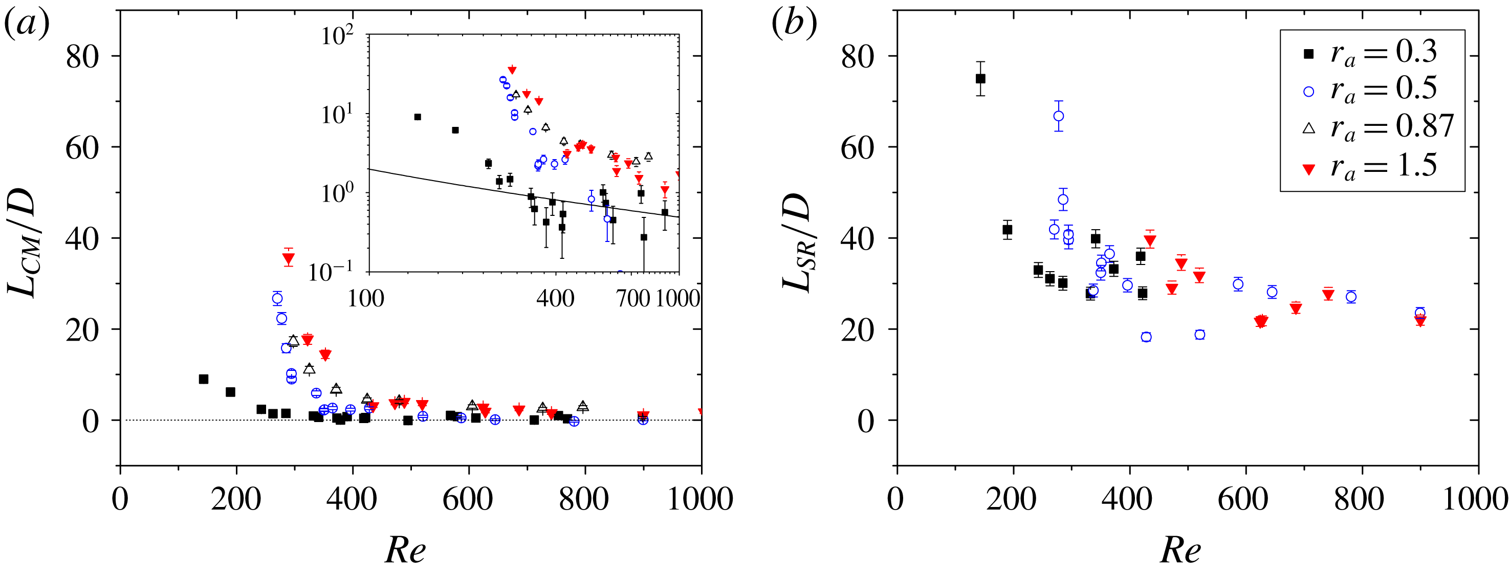
Vortex structures in figure 3 are unstable and decay downstream. We quantify the instability by measuring their spatial extents
 $L_{CM}$
and
 $L_{SR}$
, which are the length of the CM and SR parts, respectively, in the primary wake zone. In figure 4(a), we show that
 $L_{CM}/D$
approaches zero as
 $Re$
increases, indicating that the primary wake is purely SR without the appearance of CM. As seen in figure 4(b),
 $L_{SR}$
approaches an asymptotic value
 ${\sim}20D$
when
 $Re$
is high, suggesting that a finite time is required for the breakdown of the SR vortex street. We find that both
 $L_{CM}$
and
 $L_{SR}$
increase as
 $Re$
decreases, indicating that both structures are stable when
 $Re$
is small.
The spatial extents of vortex structures. The lengths of (a) the CM part (log–log plot in the inset) and (b) the SR part in the primary wake zone are plotted with respect to
 $Re$
. Both
 $L_{CM}$
and
 $L_{SR}$
approach asymptotic values, 0 and
 ${\sim}20D$
, respectively, as
 $Re$
increases, and they increase as
 $Re$
decreases. In the inset of (a), the solid line is the calculation of (3.4) for
 $r_{a}=0.3$
using
 $f=15$
.

We suspect that
 $L_{CM}$
is longer when
 $Re$
is small because the vortex broadening rate is smaller. Using (3.2), we write
 $$\begin{eqnarray}\frac{L_{CM}}{D}=(r_{K}^{(max)}-r_{K}^{(min)})\frac{U\unicode[STIX]{x1D70F}\ell }{\unicode[STIX]{x1D6FF}D},\end{eqnarray}$$
where
 $r_{K}^{(min)}=r_{K}(y=y_{0})$
and
 $r_{K}^{(max)}=r_{K}(y=y_{0}+L_{CM})$
. Using (2.1) and
 $\ell =\ell _{0}+\unicode[STIX]{x1D6FC}D$
, where
 $\ell _{0}$
is a non-zero intercept and
 $\unicode[STIX]{x1D6FC}$
is a proportionality constant (Kim & Wu Reference Kim and Wu2015), (3.3) becomes
 $$\begin{eqnarray}\frac{L_{CM}}{D}=f\,Re^{-1/2}\left(1+\frac{U\ell _{0}}{\unicode[STIX]{x1D6FC}\unicode[STIX]{x1D708}}Re^{-1}\right),\end{eqnarray}$$
where the non-dimensional coefficient
 $f=[(r_{K}^{(max)}-r_{K}^{(min)})U^{2}\unicode[STIX]{x1D70F}\unicode[STIX]{x1D6FC}]/[6\unicode[STIX]{x1D708}(r_{a}^{2}+0.25)^{1/4}]$
. It is inferred from (3.4) that
 $L_{CM}/D\propto Re^{-3/2}$
for
 $Re\ll U\ell _{0}/\unicode[STIX]{x1D6FC}\unicode[STIX]{x1D708}$
and
 $L_{CM}/D\propto Re^{-1/2}$
for
 $Re\gg U\ell _{0}/\unicode[STIX]{x1D6FC}\unicode[STIX]{x1D708}$
, where
 $U\ell _{0}/\unicode[STIX]{x1D6FC}\unicode[STIX]{x1D708}\approx 32$
, 115, 205 and 225 for
 $r_{a}=0.3$
, 0.5, 0.87 and 1.5, respectively, using the measured values of
 $\ell _{0}$
and
 $\unicode[STIX]{x1D6FC}$
. In the inset of figure 4(a), (3.4) is calculated for
 $r_{a}=0.3$
using
 $f=15$
. It is seen that when
 $Re$
is relatively large the scaling relation is roughly consistent with the measurement. However, for smaller
 $Re$
, the calculation does not match with the measurement. This discrepancy indicates that the theoretical consideration in (3.4) requires more thorough investigation.
In the second expansion zone (shaded grey in figure 3), the primary vortex street breaks down and is transformed to a secondary vortex street. This secondary expansion occurs when the primary vortex street in SR is disintegrated. Then the vortices of the primary wake are rearranged to a new vortex structure of lower frequency and longer wavelength, accompanying a rapid expansion of
 $\ell$
and a rapid decrease of
 $r_{K}$
. The final approach to the new wavelength
 $\ell _{2}$
of the secondary wake is exponential. As seen with the blue lines in figure 3(a–e),
 $\ell (y)$
in this region obeys
 $$\begin{eqnarray}\ell =\ell _{1}+(\ell _{2}-\ell _{1})(1-\text{e}^{-y/y_{2}}),\end{eqnarray}$$
where
 $y_{2}$
is a relaxation length, and our data suggest
 $y_{2}\sim \ell _{1}$
. The exponential approach is also observed in the initial expansion zone as we stated earlier, suggesting that the underlying physical mechanism of the secondary instability may not be different from that of the primary one. Also, it is inferred that
 $\ell _{1}$
of the second expansion is analogous to
 $D$
of the initial expansion.
In the secondary wake zone, the vortex street is always observed in CM under our experimental conditions. The wavelength of the newly formed vortex street
 $\ell _{2}$
is longer than the wavelength of the primary vortex street
 $\ell _{1}$
. Our measurement shows
 $\ell _{2}\simeq 10D$
, and it is stable and does not change across
 $y$
as in the primary wake zone. We note that the ratio between the two wavelengths,
 $\ell _{2}/\ell _{1}$
, is not an integer. For instance, with
 $Re=279$
, 304, 361, 537 and 665, we find
 $\ell _{2}/\ell _{1}\simeq 2.3$
, 2.4, 2.4, 2.5 and 2.4, respectively. Interestingly,
 $r_{K}$
gradually increases with
 $y$
as observed in the primary wake zone, suggesting that a sequence of transitions may occur if the channel was sufficiently long.
3.2 Stability criterion
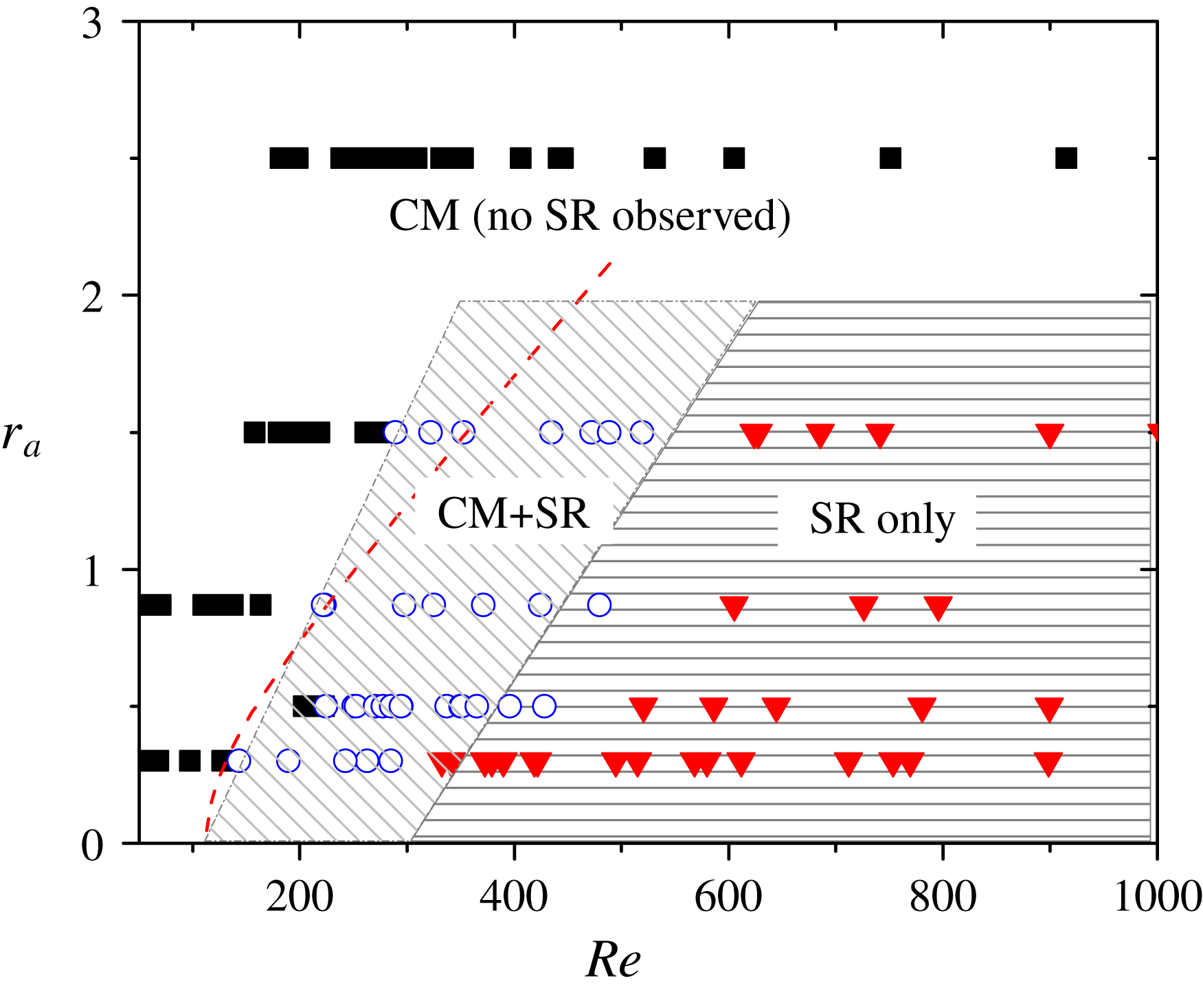
In figure 5, the structures of vortex streets in the primary wake are represented on
 $Re$
and
 $r_{a}$
plane. It shows that there exists a threshold value
 $Re_{c2}$
, such that when
 $Re<Re_{c2}$
, the vortex street is in CM and undifferentiated from the commonly observed vortex streets behind circular objects. Otherwise, when
 $Re>Re_{c2}$
, SR vortex street is observed in the primary wake zone. We define this critical Reynolds number as
 $Re_{c2}$
to distinguish it from the onset of the primary wake whose conventional symbol is
 $Re_{c}$
. This notation reflects the observation that the appearance of SR vortex street coincides with the secondary instability.
We find that
 $Re_{c2}$
is an increasing function of
 $r_{a}$
. When the rod is more streamlined, a higher
 $Re$
is required to have SR vortex structure. For instance, when we use the rod of
 $r_{a}=0.3$
, SR vortex streets are observed when
 $Re\gtrsim 130$
. However, when
 $r_{a}=1.5$
, much higher
 $Re\simeq 280$
is required to produce SR vortex streets. When
 $r_{a}=2.5$
, the vortex street is always in CM in the range of our experiments where
 $Re$
goes up to 1000.
Spatial structure of vortex streets in the primary wake zone. Each point represents the morphological structure of a vortex street created at a certain
 $r_{a}$
and
 $Re$
; a filled square indicates that the vortex street is in CM, an open circle indicates CM followed by SR and a filled triangle indicates SR without CM. The dashed line represents the calculation of (3.6).

Conversely, the observation indicates that the rods with a larger
 $r_{a}$
are less prone to form SR than the rods with a smaller
 $r_{a}$
at the same
 $Re$
or
 $D$
. For example, at
 $Re=200$
the vortex street is CM when
 $r_{a}=1.5$
but SR when
 $r_{a}=0.3$
. In the two cases, the heights of the triangles differ by a factor of five with the same
 $D$
. The flow passes by the boundary for a longer distance for the rods of higher
 $r_{a}$
, and thicker boundary layers are developed for such rods. As a result, the vortex streets are generated at different initial conditions.
From our series of experiments, we postulate that the vortex structure in the primary wake zone is determined by the dimensionless ratio
 $\unicode[STIX]{x1D6FF}/D$
. When this ratio is larger than a certain critical value
 $(\unicode[STIX]{x1D6FF}/D)_{c}$
, the vortex street is in CM. Otherwise, the primary wake is partly or entirely SR. Our analyses suggest that the critical ratio
 $(\unicode[STIX]{x1D6FF}/D)_{c}\approx 0.4$
. Using the empirical relation in (2.1), we infer that
 $$\begin{eqnarray}Re_{c2}\approx (6/0.4)^{2}\sqrt{r_{a}^{2}+0.25}=225\sqrt{r_{a}^{2}+0.25}.\end{eqnarray}$$
We mark (3.6) in figure 5 with a dashed curve and see that it roughly matches with the experimental measurement.
We test the validity of (3.6) from the runs of experiments where
 $D$
is fixed and
 $U$
is varied. We report that when the rod is
 $r_{a}=0.87$
with
 $D=0.49$
cm, the vortex street is in CM and stable where
 $U<65~\text{cm}~\text{s}^{-1}$
. Otherwise, it is destabilized by increasing
 $U$
. This result indicates that
 $Re_{c2}\simeq 240$
and is consistent with (3.6). Another run of the experiment uses the rod of
 $r_{a}=1.5$
and
 $D=1.6$
cm, and we observe that the vortex street is stabilized only when
 $U<35~\text{cm}~\text{s}^{-1}$
. For a fixed
 $D$
, the decrease of
 $U$
stabilizes the vortex streets because it makes
 $\unicode[STIX]{x1D6FF}$
thicker.
We speculate that a comprehensive understanding of wake structure requires a full consideration of instability in viscous flows. Our result seemingly contradicts the point vortex model, which assumes zero viscosity and infinitesimally thin boundary layers, in that the prediction of
 $r_{K}=0.28$
is well applicable to vortex streets from thick boundary layers. However, the viscosity plays an important role in the whole process of vortex formations including the initial expansion, broadening and vortex rearrangement. Therefore, a further theoretical consideration that takes into account the action of viscosity is an ensuing area of exploration.
4 Conclusion
We presented that vortex streets have two morphological configurations: CM and SR. Most noticeably, SR is characterized by a thin layer of irrotational fluid, which prevents the interaction between two vortex rows. On the other hand, CM is characterized by a gradual dissipation of vorticity through the interaction of two vortex rows.
We generated vortex streets in soap films by inserting triangular rods of different aspect ratios. This technique allowed us to independently adjust the thickness
 $\unicode[STIX]{x1D6FF}$
of the boundary layer and the separation distance
 $D$
between two boundary layers. We found that when
 $\unicode[STIX]{x1D6FF}/D>0.4$
, the vortex street is formed and remains in CM. Alternatively, when
 $\unicode[STIX]{x1D6FF}/D<0.4$
, the vortex street is formed in CM and then decays to SR or is formed in SR.
Our experiments demonstrate that the spatial structure of the vortex street is determined by the experimental conditions. In previous studies, SR vortex street is perceived as an interim structure that occurs only when a primary vortex street decays and is transformed to a secondary vortex street. In the present study, we find that SR vortex street is formed as an incipient vortex street under certain conditions. Our observation indicates that the vortex structure is independent of the stability condition of any arrangement.
Lastly, we presented that the primary vortex street eventually decays and is transformed to the secondary vortex street. Downstream, the secondary vortex street evolves in a fashion that is similar to that of the primary vortex street. We speculate that a sequence of transitions between CM and SR may occur. In this regard, our study of individual transitions of spatial structures may allow an understanding of the long-time evolution of vortex streets, in a larger context.
Acknowledgements
The experimental part of the study was conducted at the University of Pittsburgh while the author was a graduate student. The author thanks Professor X. L. Wu for insightful discussions.
Appendix A. Observations of boundary layers in soap films
A boundary layer is the source of vorticity for downstream flow structures, and its detachment from a solid boundary creates the initial condition for wake formation. The intensity of the vorticity in the layer and its thickness, therefore, play an important role for the current discussion.
We measure the boundary layer thickness near a thin plate inserted in flowing soap films using the video imaging technique. In this investigation, we insert the thin plate perpendicular to the film and parallel to the flow. The thickness of the thin plate is
 $25~\unicode[STIX]{x03BC}\text{m}$
, and the longitudinal length
 $L$
is varied from 0.2 to 3 cm. As the soap film flow passes by the thin plate, a boundary layer is developed to a certain thickness
 $\unicode[STIX]{x1D6FF}$
that depends on
 $L$
. In soap films, the vortical structure in the boundary layer is known to alter the thickness of the film slightly (Wu et al.
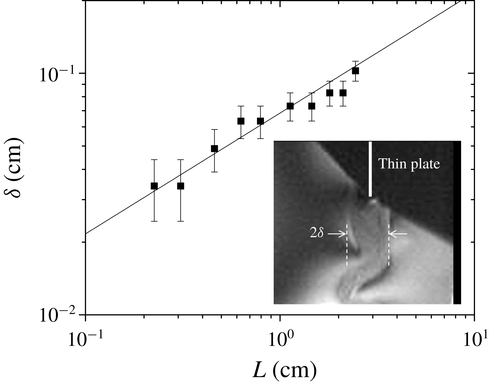
Reference Wu, Martin, Kellay and Goldburg1995; Rivera, Vorobieff & Ecke Reference Rivera, Vorobieff and Ecke1998) because the medium is slightly compressible (Kim & Mandre Reference Kim and Mandre2017), and the boundary layer is easily identified in the interferogram given that the spatial resolution is warranted. The boundary layer is shown in figure 6, and we note that the lens used for this visualization is different from the one we used for the main experiment.
The measurement of boundary layer thickness in soap films. The boundary layer thickness
 $\unicode[STIX]{x1D6FF}$
is proportional to
 $\sqrt{L}$
, where
 $L$
is the longitudinal length of a solid object inserted into the flow. The solid line is the calculation of (A 1). In the inset, an interferogram of boundary layers developed around a thin foil of
 $L=1.8$
cm (
 $\unicode[STIX]{x1D6FF}=0.083$
cm) is shown. The boundary layers are visualized because the vorticity slightly alters the thickness of the film.

In figure 6, our measurement of
 $\unicode[STIX]{x1D6FF}$
with respect to
 $L$
is presented. The measurement indicates that the boundary layer thickness in our soap film can be approximated as
 $$\begin{eqnarray}\unicode[STIX]{x1D6FF}=6\sqrt{\frac{\unicode[STIX]{x1D708}L}{U}}.\end{eqnarray}$$
The scaling relation in (A 1) is consistent with the classical boundary layer theory (Schlichting Reference Schlichting1979). We note that the proportionality constant 6 is greater than the classical value of 5. We believe that the discrepancy originates from the fact that we use the bulk viscosity value of the soap solution,
 $\unicode[STIX]{x1D708}=0.013~\text{cm}^{2}~\text{s}^{-1}$
. It is widely known that the surface viscosity of a soap film can be greater than that of the bulk (Martin & Wu Reference Martin and Wu1995; Vorobieff & Ecke Reference Vorobieff and Ecke1999; Prasad & Weeks Reference Prasad and Weeks2009; Vivek & Weeks Reference Vivek and Weeks2015).
For laminar flow passing tapered rods, we approximate the length of the plate to the length of the hypotenuse of the triangle,
 $L\simeq \sqrt{(D/2)^{2}+H^{2}}$
. Substituting
 $L$
in (A 1), the empirical equation of the boundary layer thickness in (2.1) is derived.