





1. Introduction
Rayleigh–Bénard convection (RBC) is the paradigmatic system for studying buoyancy-driven turbulence (Ahlers et al. Reference Ahlers, Grossmann and Lohse2009; Lohse & Xia Reference Lohse and Xia2010). A fluid layer is confined between two horizontal plates, heated from below and cooled from above. The dynamics is governed by two dimensionless parameters. The Rayleigh number
 $\textit{Ra}$
measures the relative importance of buoyancy to viscous and thermal diffusion. The Prandtl number (
 $\textit{Pr}$
) is the ratio of momentum to thermal diffusivity. A third parameter enters when the system is realised in a laboratory or a simulation. The geometric aspect ratio
 $\varGamma$
, defined as the ratio of the horizontal domain size to the fluid layer height, constrains the largest horizontal wavelength that the flow can accommodate. An infinite horizontal layer at given
 $\textit{Ra}$
and
 $\textit{Pr}$
admits all wavelengths. A finite
 $\varGamma$
truncates this spectrum, selecting which large-scale modes participate in the dynamics and potentially altering the scale-by-scale energy and flux balances. Most theoretical and experimental studies have focused on the dependence of heat transport on
 $\textit{Ra}$
and
 $\textit{Pr}$
, while the consequences of finite
 $\varGamma$
on the spectral dynamics of the flow have received comparatively little attention.
Grossmann & Lohse (Reference Grossmann and Lohse2000) proposed a unifying theory for the scaling of the Nusselt number (
 $\textit{Nu}$
) and Reynolds number (
 $\textit{Re}$
) by decomposing the total dissipation into boundary layer and bulk contributions. Several regimes were identified in the
 $\textit{Ra}$
vs
 $\textit{Pr}$
phase space, defined by whether the boundary layer or the bulk dominates the global kinetic and thermal dissipation. Their theory is consistent with a possible transition to the Kraichnan regime (Kraichnan Reference Kraichnan1962) (
 $\textit{Nu} \sim \textit{Ra}^{1/2}$
) at extremely large
 $\textit{Ra}$
, where the laminar boundary layer is expected to transition to turbulence. Advancement of experimental techniques has enabled much higher
 $\textit{Ra}$
than ever before. Roche et al. (Reference Roche, Gauthier, Kaiser and Salort2010) conducted RBC experiments with cryogenic helium at
 $\textit{Ra}$
up to
 $10^{12}$
in cylindrical cells with small to moderate
 $\varGamma$
. They found the side walls to have a significant role in the transition to the ultimate regime. Urban et al. (Reference Urban, Musilová and Skrbek2011) designed an improved apparatus that can attain up to
 $\textit{Ra} = 10^{15}$
while minimising parasitic heat leaks. Numerical simulations have progressed from
 $\textit{Ra} = 25\,000$
(Lipps Reference Lipps1976) to rapidly rotating RBC at
 $\textit{Ra} = 5 \times 10^{13}$
(Song et al. Reference Song, Shishkina and Zhu2024). Iyer et al. (Reference Iyer, Scheel, Schumacher and Sreenivasan2020) performed direct numerical simulations (DNS) in a slender cylindrical cell (
 $\varGamma = 1/10$
) up to
 $\textit{Ra} = 10^{15}$
and found the classical
 $\textit{Nu} \sim \textit{Ra}^{1/3}$
scaling with no transition to the ultimate regime, although the large-scale flow structure in such a slender geometry differs qualitatively from that at larger
 $\varGamma$
. Lohse & Toschi (Reference Lohse and Toschi2003) achieved the Kraichnan regime numerically by simulating only the bulk flow, eliminating both thermal and kinetic boundary layers with periodic boundary conditions. These high-
 $\textit{Ra}$
experiments and simulations have predominantly been performed at small
 $\varGamma$
, however, because the computational and experimental cost grows rapidly with the domain size.
The aspect ratio has a profound effect on the large-scale organisation of the flow. A characteristic feature of turbulent RBC at moderate
 $\varGamma$
(of order unity) is the spontaneous formation of a large-scale circulation, a coherent mean flow that spans the height of the cell (Krishnamurti & Howard Reference Krishnamurti and Howard1981; Ahlers et al. Reference Ahlers, Grossmann and Lohse2009). The large-scale circulation generally appears as a single fluid loop that rises on one side and descends on the opposite side, shearing the thermal boundary layers (Xi et al. Reference Xi, Lam and Xia2004; Sun et al. Reference Sun, Xia and Tong2005). Its strength and orientation are dynamic, displaying cessations and complete reversals (Brown & Ahlers Reference Brown and Ahlers2006; Xi & Xia Reference Xi and Xia2008). The topology of the large-scale circulation changes qualitatively as
 $\varGamma$
increases. The single-roll structure transitions to multiple coexisting rolls and eventually to ‘turbulent superstructures,’ extensive thermal patterns that stretch horizontally over many cell heights (Pandey et al. Reference Pandey, Scheel and Schumacher2018; Stevens et al. Reference Stevens, Blass, Zhu, Verzicco and Lohse2018). Krug et al. (Reference Krug, Lohse and Stevens2020) showed that these superstructures exhibit strong coherence between the temperature and velocity fields and carry a significant fraction of the convective heat flux. Stevens et al. (Reference Stevens, Hartmann, Verzicco and Lohse2024) performed DNS over a wide range of
 $\varGamma$
and found that integral quantities such as
 $\textit{Nu}$
converge by
 $\varGamma \approx 4$
, but the flow structure itself, particularly the temperature and velocity variance distributions, remains sensitive to
 $\varGamma$
up to
 $\varGamma \approx 8$
. The large-scale circulation and superstructures play a central role in global heat transport because the Nusselt number is directly determined by the covariance of vertical velocity and temperature,
 $\langle w\theta \rangle$
, which these large-scale modes organise. How the spectral content of
 $\langle w\theta \rangle$
and its governing budget change with
 $\varGamma$
is therefore a central question.
The organisation of turbulence into coherent large-scale patterns is a universal feature of bounded turbulence, not unique to thermally driven flows. Kim & Adrian (Reference Kim and Adrian1999) identified ‘very large-scale motions’ (VLSMs) in turbulent pipe flow, long meandering regions of streamwise velocity fluctuation extending up to 12–14 pipe radii. Hutchins & Marusic (Reference Hutchins and Marusic2007) revealed ‘superstructures’ in turbulent boundary layers exceeding 20 boundary layer thicknesses in length. This structural organisation is perhaps most pronounced in plane Couette flow, where the constant shear across the entire gap causes extremely long streamwise streaks (Komminaho et al. Reference Komminaho, Lundbladh and Johansson1996; Kitoh & Umeki Reference Kitoh and Umeki2008). Lee & Moser (Reference Lee and Moser2018) showed that these structures can have streamwise extents exceeding
 $310\delta$
(where
 $\delta$
is the half-gap width) and that their presence is apparent in the spectra of all velocity components and the Reynolds stress. Plane Couette flow shares a deeper analogy with RBC. Both flows are driven by a constant forcing across the entire gap (shear in one case, buoyancy in the other), both lack a centreline symmetry that would suppress the largest scales and both produce domain-filling structures that carry a disproportionate fraction of the conserved flux. The role of large-scale modes in these shear flows is functionally analogous to that of the large-scale circulation and superstructures in RBC. They dominate the transport of momentum (Reynolds stress) in shear flows much like the large-scale modes dominate the transport of heat (
 $\langle w\theta \rangle$
) in convection (Smits et al. Reference Smits, McKeon and Marusic2011). The scale and character of these structures in shear flows are also sensitive to the computational domain size, paralleling the
 $\varGamma$
dependence in RBC. The spectral methodology developed for shear flows therefore provides a natural framework for investigating heat transport in RBC.
Single-point statistics provide essential information about the global state of the flow but effectively average over scales, obscuring the hierarchy of interactions that govern transport and dissipation (Tennekes & Lumley Reference Tennekes and Lumley1972; Pope Reference Pope2000). Spectral decomposition is necessary to resolve these interactions. Kim & Adrian (Reference Kim and Adrian1999) and Hutchins & Marusic (Reference Hutchins and Marusic2007) used premultiplied energy spectra to identify VLSMs and superstructures, demonstrating that the spectral peaks of momentum transport are distinct from those of turbulent production. Lee & Moser (Reference Lee and Moser2015) provided a comprehensive spectral dataset for channel flow up to
 $\textit{Re}_\tau \approx 5200$
, and Mizuno (Reference Mizuno2016) and Cho et al. (Reference Cho, Hwang and Choi2018) examined the spectra of energy transport to reveal how turbulence is redistributed spatially and across scales. Lee & Moser (Reference Lee and Moser2019) performed a spectral analysis of the budget equations for turbulent kinetic energy and Reynolds stress, identifying transport mechanisms that were invisible to single-point statistics. This methodology of closing the budget equations in spectral space provides the framework for decoupling the dynamics of large-scale production from small-scale dissipation.
The budget equation of
 $\langle w\theta \rangle$
is of particular importance in RBC because
 $\langle w\theta \rangle$
directly determines the Nusselt number and, hence, the global heat transport. This budget describes the balance among production, turbulent transport, pressure–temperature interaction and molecular terms. Wyngaard et al. (Reference Wyngaard, Coté and Izumi1971) derived and experimentally investigated this budget in the atmospheric surface layer under convective conditions. Otić & Grötzbach (Reference Otić and Grötzbach2007) analysed the same budget using DNS of RBC in liquid lead–bismuth at a low Prandtl number. In physical space, Wang et al. (Reference Wang, He and Tong2016, Reference Wang, Xu, He, Yik, Wang, Schumacher and Tong2018) derived and experimentally validated budget equations for the mean and variance temperature profiles in which the velocity–temperature correlations
 $\langle w\theta \rangle$
and
 $\langle w\theta ^2\rangle$
enter explicitly, providing an equation-based description of the production, transport, diffusion and dissipation associated with boundary layer fluctuations and of the distinction between boundary layer and mixing-zone dynamics. In scale space, Togni et al. (Reference Togni, Cimarelli and De Angelis2015) derived exact scale-by-scale balances for the kinetic energy and temperature variance in RBC, identifying multiscale transport and reverse-transfer behaviour near the walls, and Togni et al. (Reference Togni, Cimarelli and De Angelis2019) extended this framework to the resolved and subgrid dynamics relevant to large-eddy simulation. The spectral budget considered here complements these physical-space and scale-space formulations by resolving the budget of
 $\langle w\theta \rangle$
, the covariance that directly determines
 $\textit{Nu}$
, simultaneously in horizontal wavelength and vertical location. Lee (Reference Lee2024) performed a spectral analysis of this budget in RBC at three Rayleigh numbers, each at a single large aspect ratio. That study established the spectral framework, identified the two-peak structure of the premultiplied spectra and concluded that large-scale structures play a crucial role in the dynamics of
 $\langle w\theta \rangle$
, but have a minimal impact on the Nusselt number scaling. The analysis was restricted to a single
 $\varGamma$
, however, and could not address how the spectral budget changes as the domain transitions from one that suppresses superstructures to one that fully accommodates them. A systematic investigation of how the spectral budget depends on
 $\varGamma$
across multiple
 $\textit{Ra}$
has not been carried out.
The aspect ratio dictates the available phase space for large-scale modes and is therefore expected to fundamentally restructure the scale-by-scale balance of production, transport and destruction in the
 $\langle w\theta \rangle$
budget. We address this question by extending the single-aspect-ratio analysis of Lee (Reference Lee2024) to a systematic variation of
 $\varGamma$
. Direct numerical simulation is performed at three Rayleigh numbers with up to three different aspect ratios each, yielding eight cases in total (the smallest aspect ratio at
 $\textit{Ra} = 1\times 10^5$
is excluded because the domain is too narrow to sustain turbulent convection at this
 $\textit{Ra}$
and the flow relaminarises). The spectral distributions of production, transport, pressure–temperature interaction and molecular terms are explicitly computed and analysed to determine which scales contribute to the vertical heat flux and how these contributions change with
 $\varGamma$
. This parametric study reveals findings that are inaccessible at a single
 $\varGamma$
, including the reversal of the inter-scale cascade direction with
 $\varGamma$
, the cancellation of large-scale pressure transport by the pressure–strain term, and a complete term-by-term demonstration that no budget mechanism delivers large-scale spectral content into the thermal boundary layer. In particular, the inter-scale transfer of the covariance is shown to constitute a net upscale flux while the kinetic energy and the temperature variance cascade towards small scales, consistent with the strong large-scale coherence between the velocity and temperature fields, which is the defining property of the superstructures (Krug et al. Reference Krug, Lohse and Stevens2020). The contribution of the present work is thus specific. Building on the physical-space formulations of Wang et al. (Reference Wang, He and Tong2016, Reference Wang, Xu, He, Yik, Wang, Schumacher and Tong2018) and the scale-space balances of Togni et al. (Reference Togni, Cimarelli and De Angelis2015, Reference Togni, Cimarelli and De Angelis2019), it derives and evaluates the spectral budget of the heat-flux covariance
 $\langle w\theta \rangle$
itself and quantifies its dependence on the aspect ratio. The primary objective is to establish the spectral mechanisms through which the aspect ratio controls the dynamics of
 $\langle w\theta \rangle$
and the global heat transport.
The remainder of this paper is organised as follows. The numerical methodology, the governing equations and the statistical convergence of the simulated datasets are detailed in § 2. The results of the spectral analysis are presented in § 3, offering a detailed breakdown of the budget terms for
 $\langle w\theta \rangle$
and discussing the physical implications of the aspect ratio dependence. The findings are summarised in § 4.
2. Method
2.1. Numerical method
The
 $x$
(or
 $x_1$
) and
 $y$
(or
 $x_2$
) directions are the homogeneous directions. The
 $z$
(or
 $x_3$
) direction is the vertical direction. The corresponding velocities are
 $U$
(or
 $U_1$
) and
 $V$
(or
 $U_2$
) for homogeneous directions and
 $W$
(or
 $U_3$
) for the vertical direction. The operator
 $\langle \boldsymbol{\cdot }\rangle$
denotes the expectation or average of a quantity over the homogeneous directions and time, at a fixed vertical location
 $z$
, and the lower case denotes fluctuations about the expectation, i.e.
 $U = \langle U \rangle + u$
and
 $\langle u \rangle = 0$
.
The normalised governing equations for the incompressible Rayleigh–Bénard flows are
 \begin{equation} \begin{aligned} \frac {\partial U_k}{\partial x_k} &= 0, \\ \frac {\partial U_i}{\partial t} &= -\frac {\partial U_i U_k}{\partial x_k} + \sqrt {\frac {\textit{Pr}}{\textit{Ra}}} \frac {\partial ^2 U_i}{\partial x_k \partial x_k}- \frac {\partial p}{\partial x_i} + \varTheta \delta _{i3}, \\ \frac {\partial \varTheta }{\partial t} &= -\frac {\partial \varTheta U_k}{\partial x_k} + \frac {1}{\sqrt {\textit{PrRa}}} \frac {\partial ^2 \varTheta }{\partial x_k \partial x_k}. \end{aligned} \end{equation}
The Prandtl number is the ratio of kinematic viscosity
 $\nu$
to thermal diffusivity
 $\alpha$
, i.e.
 $\textit{Pr} = \nu /\alpha$
. The Rayleigh number
 $\textit{Ra}$
is defined as
 $\textit{Ra} = \beta g \Delta _T H^3 / (\nu \alpha )$
, where
 $\beta$
is the thermal expansion coefficient,
 $g$
is the gravitational acceleration constant,
 $\Delta _T$
is the temperature difference between the top and bottom planes, and
 $H$
is the distance between the planes. The coordinates
 $x_i$
are normalised by
 $H$
and
 $\varTheta$
is the temperature normalised by
 $\Delta _T$
. The time
 $t$
, velocity
 $U_i$
and pressure
 $p$
are normalised by
 $\sqrt {H/(g\beta \Delta _T)}$
,
 $\sqrt {g\beta \Delta _T H}$
and
 $\rho _0 g \beta \Delta _T H$
, respectively, where
 $\rho _0$
is the reference density.
The velocity–vorticity formulation of Kim et al. (Reference Kim, Moin and Moser1987) is adopted for computational efficiency. The state variables in this formulation are
 $\varOmega _z$
,
 $\varPhi$
and
 $\varTheta$
, where
 $\varOmega _z$
is the vertical vorticity and
 $\varPhi$
is the Laplacian of vertical velocity defined as follows:
 \begin{align} \varOmega _z &= \frac {\partial V}{\partial x} - \frac {\partial U}{\partial y}, \\[-12pt]\nonumber \end{align}
 \begin{align} \varPhi &= \frac {\partial ^2 W }{\partial x_k \partial x_k} = {\nabla} ^2 W. \end{align}
Equation (2.1) then becomes
 \begin{equation} \frac {\partial \mathbf{\varPhi }}{\partial t} = \boldsymbol{N} + \boldsymbol{L}, \end{equation}
where
 \begin{equation} \begin{aligned} \mathbf{\varPhi } =& \{\varTheta , \; \varOmega _z,\; \varPhi \},\\[3pt] \boldsymbol{N} =& \left \{-\frac {\partial \varTheta U_k}{\partial x_k}, \; \frac {\partial ^2 U U_k}{\partial y \partial x_k} -\frac {\partial ^2 V U_k}{\partial x \partial x_k}, -\frac {\partial ^3 W U_k}{\partial x_j \partial x_j \partial x_k} + \frac {\partial ^3 U_j U_k}{\partial z \partial x_j \partial x_k} + \frac {\partial ^2 \varTheta }{\partial x^2} + \frac {\partial ^2 \varTheta }{\partial y^2} \right \}\!,\\[3pt] \boldsymbol{L} =& \left \{\frac {1}{\sqrt {\textit{PrRa}}}{\nabla} ^2 \varTheta , \;\sqrt {\frac {\textit{Pr}}{\textit{Ra}}}{\nabla} ^2 \varOmega _z,\;\sqrt {\frac {\textit{Pr}}{\textit{Ra}}}{\nabla} ^2 \varPhi \right \}\!. \end{aligned} \end{equation}
Equations (2.1) and (2.4) are equivalent, but (2.4) is computationally beneficial because the numerical operators are the same for all state variables. The implicit and explicit (IMEX) Runge–Kutta method of Spalart et al. (Reference Spalart, Moser and Rogers1991) is used for time advancement. The spectral-Galerkin method is used for spatial derivatives in the homogeneous directions and the seventh-order B-spline collocation method is used in the vertical direction. Aliasing from second-order products is eliminated by applying Orszag’s 3/2 rule with zero padding (Orszag Reference Orszag1971). The simulations are performed with a modified version of our in-house simulation code that has been used for Lee & Moser (Reference Lee and Moser2015, Reference Lee and Moser2018). Details of the simulation code implementation can be found in Lee et al. (Reference Lee, Malaya and Moser2013, Reference Lee, Ulerich, Malaya and Moser2014).
Simulation parameters:
 $\varGamma = L/H$
is the aspect ratio, where
 $L$
is the simulation domain size in the homogeneous directions and
 $H$
is the distance between walls;
 $N_\|$
is the number of grid points in the spectral domain,
 $N_\bot$
is the number of collocation points in the vertical direction,
 $\eta$
is the grid-stretch parameter in the vertical direction,
 $\textit{Re}_\|$
is the horizontal Reynolds number,
 $\textit{Re}_\bot$
is the vertical Reynolds number,
 $\textit{Re}_T$
is the total Reynolds number and
 $\delta _\theta$
is the thermal boundary layer thickness.

Table 1. Long description
The table presents simulation parameters for various cases, detailing aspects like the aspect ratio, simulation domain size, number of grid points, collocation points, grid-stretch parameter, and Reynolds numbers. It includes eight rows and ten columns. Column headers are Case, Ra, Γ, N||, N⊥, η, Nu, Re||, Re⊥, ReT, and δθ. Row labels are case identifiers. Each row lists specific values for each parameter. Notable trends include variations in Reynolds numbers and grid points across different cases.
The pressure field does not need to be computed to advance the simulation in time. It is computed for analysis by solving the following Poisson equation from the existing velocity fields:
 \begin{equation} \frac {\partial ^2 P}{\partial x_i\partial x_i} = -\frac {\partial ^2 U_i U_k}{\partial x_i \partial x_k} + \frac {\partial \varTheta }{\partial z}. \end{equation}
The boundary condition at the wall is
 \begin{equation} \frac {\partial P}{\partial z} = \sqrt {\frac {\textit{Pr}}{\textit{Ra}}} \frac {\partial ^2 W}{\partial z^2} + \varTheta . \end{equation}
The mean pressure profile is computed with
 \begin{equation} \langle P\rangle = -\langle W^2 \rangle + \int _0^z \langle \varTheta \rangle \mathrm{d} z. \end{equation}
2.2. Simulation cases
Eight cases at different
 $\textit{Ra}$
and domain aspect ratios are simulated. The aspect ratio is defined as
 $\varGamma = L/H$
, where
 $L$
is the horizontal period of the domain. Its value for each case is listed in table 1. The Prandtl number is fixed at unity because the role of
 $\textit{Pr}$
is beyond the scope of this study. The simulation parameters are summarised in table 1. The knot locations for the seventh-order B-spline in the vertical direction are assigned with the function
 \begin{equation} z_n^{\textit{knot}} = \frac 12 \left (\frac {\displaystyle \sin \left [ \left (\frac {2(n-1)}{N_\bot -7} -1\right ) \frac {\eta \pi }{2}\right ]}{ \displaystyle \sin \left (\frac {\eta \pi }{2}\right ) }+1 \right )\!, \end{equation}
where
 $n = 1,2, {\cdots} , N_\bot -6$
and
 $\eta$
is the grid-stretch parameter that controls the clustering of the knots towards the walls. Its value for each case is listed in table 1. Greville abscissae are used to obtain the collocation points in the vertical direction (Johnson Reference Johnson2005). Table 1 also includes the Nusselt number, the homogeneous (
 $\textit{Re}_\|$
), vertical (
 $\textit{Re}_\bot$
) and total Reynolds numbers (
 $\textit{Re}_T$
), and the thermal boundary layer thickness (
 $\delta _\theta$
) for comparison with the values from Krug et al. (Reference Krug, Lohse and Stevens2020). These quantities are defined as
 \begin{equation} \textit{Nu} = \sqrt {\textit{PrRa}}\langle w \theta \rangle - \frac {\partial \langle \varTheta \rangle }{\partial z}, \end{equation}
 \begin{align} \textit{Re}_\| &= \left [\frac {\textit{Ra}}{\textit{Pr}} \int _0^1 \langle u^2 + v^2 \rangle \mathrm{d}z \right ]^{1/2}\!, \end{align}
 \begin{align} \textit{Re}_\bot &= \left [\frac {\textit{Ra}}{\textit{Pr}} \int _0^1 \langle w^2 \rangle \mathrm{d}z \right ]^{1/2}\!, \end{align}
 \begin{align} \textit{Re}_T &= \left [\frac {\textit{Ra}}{\textit{Pr}} \int _0^1 \langle u^2 + v^2 + w^2 \rangle \mathrm{d}z \right ]^{1/2}\!, \end{align}
 \begin{equation} \delta _\theta = \frac {1}{2 \textit{Nu}}. \end{equation}
The variations as functions of
 $\textit{Ra}$
follow the same trend (not shown), although some values of
 $\textit{Ra}$
in the current work differ from those in Krug et al. (Reference Krug, Lohse and Stevens2020).
The spatial resolution is assessed a posteriori from the spectral densities of the budget terms. The terms involving molecular transport, namely the molecular diffusion and the non-diffusive molecular term, are precisely the terms whose spectral content is concentrated at the smallest scales of the flow, so insufficient resolution would manifest as an accumulation of spectral density near the grid cutoff. As shown in § 3.6, the spectral densities decay to negligible values by the smallest resolved wavelength at
 $\textit{Ra} = 1\times 10^5$
. At
 $\textit{Ra} = 6\times 10^6$
and
 $4\times 10^8$
the densities of the non-diffusive molecular terms are not fully closed at the smallest resolved scales. The residual level is, however, small compared with the dominant spectral content, and all dynamically meaningful structures of the budget, that is, the spectral peaks and the production, transport and destruction regions, lie well within the resolved range. The mildness of the small-scale accumulation indicates that the unresolved contribution is negligible for the quantities analysed in this study. The number of collocation points within the thermal boundary layer (
 $z \lt \delta _\theta$
) is 22 at
 $\textit{Ra} = 1\times 10^5$
, 33–34 at
 $6\times 10^6$
and 36–37 at
 $4\times 10^8$
. At
 $\textit{Pr} = 1$
the viscous boundary layer has the same thickness, so the same counts apply.
Instantaneous temperature fields for the three large-aspect-ratio cases are shown in figure 1. The warm rising and cold descending fluid, and the horizontal patterns spanning many layer heights that constitute the thermal superstructures, are directly visible, and the growth of these patterns with
 $\textit{Ra}$
can be compared across the panels.
Instantaneous temperature fields for the large-aspect-ratio cases
 $1\mathrm{E}5\mathrm{L}$
(a),
 $6\mathrm{E}6\mathrm{L}$
(b) and
 $4\mathrm{E}8\mathrm{L}$
(c). The
 $1\mathrm{E}5\mathrm{L}$
field is cropped to the same horizontal extent as the other two cases for comparison. Its full domain is twice as wide (
 $\varGamma = 31.4$
). Warm (rising) fluid appears in yellow–orange and cold (descending) fluid in green–blue. The horizontal patterns spanning many layer heights are the thermal superstructures whose spectral signature is analysed in § 3.

2.3. Spectral analysis of the budget equations
The terms in the evolution equation of the spectral density of
 $\langle w \theta \rangle$
are derived and defined here. The Reynolds decomposition is first applied to the velocity, pressure and temperature:
 \begin{align} U_i &= \langle U_i \rangle +u_i, \\[-12pt]\nonumber \end{align}
 \begin{align} P &= \langle P \rangle + p, \\[-12pt]\nonumber \end{align}
 \begin{align} \varTheta &= \langle \varTheta \rangle +\theta . \end{align}
The mean velocity components are all zero for plane RBC:
 \begin{equation} \langle U_i \rangle = 0. \end{equation}
The continuity equation gives
 \begin{equation} \frac {\partial u_k}{\partial x_k} = 0. \end{equation}
The evolution equations for
 $w$
and
 $\tilde \theta$
are obtained using (2.14) and (2.15):
 \begin{align} \frac {\partial w}{\partial t} &= -\frac {\partial w u_k}{\partial x_k}+\frac {\partial \langle w^2\rangle }{\partial z} + \sqrt {\frac {\textit{Pr}}{\textit{Ra}}} \frac {\partial ^2 w}{\partial x_k \partial x_k} - \frac {\partial p}{\partial z} + \theta , \\[-12pt]\nonumber \end{align}
 \begin{align} \frac {\partial {\tilde \theta }}{\partial t} &= -\widetilde {\frac {\partial {\theta u_k}}{\partial x_k}}+ \frac {\partial \langle w\theta \rangle }{\partial z} + \frac {1}{\sqrt {\textit{PrRa}}} \widetilde {\frac {\partial ^2 \theta }{\partial x_k \partial x_k}}-\tilde w\frac {\partial \langle \varTheta \rangle }{\partial z}. \end{align}
Here the separation vectors with separation distance
 $\boldsymbol{r}$
in the homogeneous directions are defined as
 \begin{align} \tilde u_i &= u_i(\boldsymbol{x} + \boldsymbol{r}), \\[-12pt]\nonumber \end{align}
 \begin{align} \tilde p &= p(\boldsymbol{x} + \boldsymbol{r}), \\[-12pt]\nonumber \end{align}
 \begin{align} \tilde \theta &= \theta (\boldsymbol{x} + \boldsymbol{r}). \end{align}
The position vector is
 $\boldsymbol{x} = (x, y ,z)$
, the separation vector is
 $\boldsymbol{r} = (r_x, r_y , 0)$
, and
 $r_x$
and
 $r_y$
are separation distances in the homogeneous directions.
The two-point correlation function of
 $w$
and
 $\theta$
is
 $R^{w\theta }(r_x, r_y, z) = \langle w \tilde \theta \rangle$
. Its evolution equation is obtained by multiplying
 $w$
and
 $\tilde \theta$
with (2.17) and (2.16), respectively, and taking expectations of their summation:
 \begin{equation} \begin{aligned} \frac {\partial R^{w\theta }}{\partial t} =& \left \langle \tilde \theta \frac {\partial w}{\partial t} \right \rangle + \left \langle w\frac {\partial \tilde \theta }{\partial t} \right \rangle \\ =& -\left \langle \tilde \theta \frac {\partial w u_k}{\partial x_k} \right \rangle -\left \langle w\widetilde {\frac {\partial \theta u_k}{\partial x_k}}\right \rangle + \sqrt {\frac {\textit{Pr}}{\textit{Ra}}} \left \langle \tilde \theta \frac {\partial ^2 w}{\partial x_k \partial x_k} \right \rangle + \frac {1}{\sqrt {\textit{PrRa}}} \left \langle w\widetilde {\frac {\partial ^2 \theta }{\partial x_k \partial x_k}}\right \rangle \\ & - \left \langle \tilde \theta \frac {\partial p}{\partial z} \right \rangle + \big \langle \theta \tilde \theta \big \rangle -\langle w\tilde w \rangle \frac {\partial \langle \varTheta \rangle }{\partial z},\end{aligned} \end{equation}
 \begin{equation} \frac {\partial R^{w\theta }}{\partial t} = R^{w\theta }_T + R^{w\theta }_{\alpha } + R^{w\theta }_{\varPi } + R^{w\theta }_{P}. \end{equation}
Here
 $R^{w\theta }_T$
is the turbulent transport,
 $R^{w\theta }_{\alpha }$
is the molecular term arising from viscous and thermal diffusion,
 $R^{w\theta }_\varPi$
is the pressure–temperature interaction and
 $R^{w\theta }_P$
is the production. These terms are defined as
 \begin{align} R^{w\theta }_T &= -\left \langle \tilde \theta \frac {\partial w u_k}{\partial x_k} \right \rangle -\left \langle w\widetilde {\frac {\partial \theta u_k}{\partial x_k}}\right \rangle \!, \\[-12pt]\nonumber \end{align}
 \begin{align} R^{w\theta }_{\alpha } &= \sqrt {\frac {\textit{Pr}}{\textit{Ra}}} \left \langle \tilde \theta \frac {\partial ^2 w}{\partial x_k \partial x_k} \right \rangle + \frac {1}{\sqrt {\textit{PrRa}}} \left \langle w\widetilde {\frac {\partial ^2 \theta }{\partial x_k \partial x_k}}\right \rangle \!, \\[-12pt]\nonumber \end{align}
 \begin{align} R^{w\theta }_{\varPi } &= - \left \langle \tilde \theta \frac {\partial p}{\partial z} \right \rangle \!, \\[-12pt]\nonumber \end{align}
 \begin{align} R^{w\theta }_{P} &= \big \langle \theta \tilde \theta \big \rangle -\langle w\tilde w \rangle \frac {\partial \langle \varTheta \rangle }{\partial z}. \end{align}
The turbulent transport
 $R^{w\theta }_T$
represents the advection of
 $R^{w\theta }$
by velocity fluctuations. The molecular term
 $R^{w\theta }_{\alpha }$
accounts for the effects of viscous diffusion acting on the vertical velocity
 $w$
and of thermal diffusion acting on the temperature fluctuation
 $\theta$
. The pressure–temperature term
 $R^{w\theta }_\varPi$
represents the interaction between pressure and temperature fluctuations through the vertical pressure gradient. The production term
 $R^{w\theta }_P$
consists of two contributions. The first,
 $\langle \theta \tilde \theta \rangle$
, is the buoyancy production arising from the temperature variance. The second,
 $-\langle w \tilde w\rangle \partial \langle \varTheta \rangle /\partial z$
, is the production by the mean temperature gradient.
These terms can be further decomposed. The turbulent transport is split into the vertical transport
 $R^{w\theta }_{T^\bot }$
and the inter-scale transfer in the homogeneous directions
 $R^{w\theta }_{T^\|}$
:
 \begin{align} R^{w\theta }_T &= R^{w\theta }_{T^\bot } + R^{w\theta }_{T^\|}, \\[-12pt]\nonumber \end{align}
 \begin{align} R^{w\theta }_{T^\bot } &= -\frac 12 \frac {\partial \langle \tilde \theta w^2 \rangle }{\partial z} -\frac 12 \frac {\partial \langle w \widetilde {\theta w}\rangle }{\partial z}, \\[-12pt]\nonumber \end{align}
 \begin{align} R^{w\theta }_{T^\|} &= -\left \langle \tilde \theta \frac {\partial w u_k}{\partial x_k} \right \rangle -\left \langle w\widetilde {\frac {\partial \theta u_k}{\partial x_k}}\right \rangle + \frac 12 \frac {\partial \langle \tilde \theta w^2 \rangle }{\partial z} +\frac 12 \frac {\partial \langle w \widetilde {\theta w}\rangle }{\partial z}. \end{align}
The vertical transport
 $R^{w\theta }_{T^\bot }$
represents the spatial redistribution of
 $R^{w\theta }$
in the
 $z$
direction by turbulent fluctuations. The inter-scale transfer
 $R^{w\theta }_{T^\|}$
represents the transfer of
 $R^{w\theta }$
across different length scales in the homogeneous directions through nonlinear interactions.
The pressure–temperature term is decomposed into the pressure transport
 $R^{w\theta }_{\varPi ,d}$
and the pressure strain
 $R^{w\theta }_{\varPi ,s}$
:
 \begin{align} R^{w \theta }_\varPi &= R^{w \theta }_{\varPi , d} + R^{w \theta }_{\varPi , s}, \\[-12pt]\nonumber \end{align}
 \begin{align} R^{w \theta }_{\varPi , d} &= -\frac {\partial \langle p \tilde {\theta }\rangle }{\partial z}, \\[-12pt]\nonumber \end{align}
 \begin{align} R^{w \theta }_{\varPi , s} &= \left \langle p \frac {\partial \tilde {\theta }}{\partial z} \right \rangle \!. \end{align}
The pressure transport
 $R^{w\theta }_{\varPi ,d}$
redistributes
 $R^{w\theta }$
spatially in the vertical direction through the correlation between pressure and temperature fluctuations. The term
 $R^{w\theta }_{\varPi ,s}$
is the remainder of the pressure–temperature interaction after the transport contribution is separated. The label ‘pressure strain’ is adopted by analogy with the Reynolds stress budget, where a similar decomposition yields the pressure–strain correlation involving velocity gradients. The analogy is not exact. The Reynolds stress pressure–strain term involves the strain rate (velocity gradient) and redistributes energy among different components of the stress tensor. The term
 $R^{w\theta }_{\varPi ,s}$
involves the vertical temperature gradient
 $\partial \tilde \theta /\partial z$
rather than a velocity gradient and acts on the scalar flux
 $\langle w\theta \rangle$
rather than on a tensor. This term does not integrate to zero over the vertical direction, so it can act as a net source or sink of
 $R^{w\theta }$
when integrated in
 $z$
. Physically, it represents the decorrelation or correlation between
 $w$
and
 $\theta$
mediated by pressure fluctuations. The pressure field couples the velocity and temperature fields through the Poisson equation, and
 $R^{w\theta }_{\varPi ,s}$
quantifies this coupling at each scale and vertical location.
The molecular term
 $R^{w\theta }_{\alpha }$
is decomposed into the molecular diffusion
 $R^{w\theta }_{D}$
, which acts as a vertical diffusion, and the non-diffusive molecular term
 $R^{w\theta }_{\epsilon }$
:
 \begin{align} R^{w\theta }_{\alpha } &= R^{w\theta }_{D} - R^{w\theta }_{\epsilon }, \\[-12pt]\nonumber \end{align}
 \begin{align} R^{w\theta }_{D} &= \sqrt {\frac {\textit{Pr}}{\textit{Ra}}} \frac {\partial ^2 \langle w \tilde \theta \rangle }{\partial z^2} + \frac {1}{\sqrt {\textit{PrRa}}} \frac {\partial ^2 \langle w \tilde \theta \rangle }{\partial z^2}, \\[-12pt]\nonumber \end{align}
 \begin{align} R^{w\theta }_{\epsilon } &= - \sqrt {\frac {\textit{Pr}}{\textit{Ra}}} \left \langle \tilde \theta \frac {\partial ^2 w}{\partial x_k \partial x_k} \right \rangle -\frac {1}{\sqrt {\textit{PrRa}}} \left \langle w\widetilde {\frac {\partial ^2 \theta }{\partial x_k \partial x_k}}\right \rangle + \left ( \sqrt {\frac {\textit{Pr}}{\textit{Ra}}} + \frac {1}{\sqrt {\textit{PrRa}}}\right ) \frac {\partial ^2 \langle w \tilde \theta \rangle }{\partial z^2}. \end{align}
Here,
 $R^{w\theta }_{D}$
is the molecular diffusion that spatially redistributes
 $R^{w\theta }$
in the
 $z$
direction. The term
 $R^{w\theta }_{\epsilon }$
is the non-diffusive molecular term, defined as the negative of the part of
 $R^{w\theta }_{\alpha }$
that remains after the vertical diffusion
 $R^{w\theta }_{D}$
is removed (
 $R^{w\theta }_{\epsilon } = R^{w\theta }_{D} - R^{w\theta }_{\alpha }$
). It therefore enters the budget with a negative sign, so that positive
 $R^{w\theta }_{\epsilon }$
acts as a sink of
 $R^{w\theta }$
and negative
 $R^{w\theta }_{\epsilon }$
as a source. Unlike the dissipation in the turbulent kinetic energy budget, it involves cross-correlations between velocity and temperature rather than a squared quantity, so it is not sign-definite and is not a dissipation in the variance sense. The subscript
 $\epsilon$
is retained by analogy with the decomposition of the Reynolds stress budget (Lee & Moser Reference Lee and Moser2019), where the viscous term is similarly split into a vertical diffusion and a remainder that corresponds to the dissipation. At zero separation (
 $\boldsymbol{r} = \boldsymbol{0}$
),
 $R^{w\theta }_{D} - R^{w\theta }_{\epsilon }$
reduces to the molecular terms of the one-point budget of
 $\langle w\theta \rangle$
(2.42). Even at zero separation,
 $R^{w\theta }_{\epsilon }$
is not sign-definite because it involves cross-correlations of gradients (e.g.
 $\langle \partial w / \partial x_k \boldsymbol{\cdot }\partial \theta / \partial x_k \rangle$
) rather than squared gradients, so it is not guaranteed to act as a sink.
The two-point correlation
 $R^{w\theta }(\boldsymbol{r}, z)$
and the one-point covariance
 $\langle w\theta \rangle (z)$
are related by
 \begin{equation} R^{w\theta }(\boldsymbol{0}, z) = \langle w\theta \rangle (z). \end{equation}
The cross-spectral density
 $E^{w\theta }(\boldsymbol{\kappa }, z)$
is obtained by the Fourier transform of
 $R^{w\theta }$
with respect to the separation vector
 $\boldsymbol{r}$
:
 \begin{equation} E^{w\theta }(\boldsymbol{\kappa }, z) = \frac {1}{(2\pi )^2}\int _{-\infty }^{\infty }\int _{-\infty }^{\infty } R^{w\theta }(\boldsymbol{r}, z) \, e^{-\mathrm{i}\boldsymbol{\kappa }\boldsymbol{\cdot }\boldsymbol{r}} \,\mathrm{d}r_x \,\mathrm{d}r_y. \end{equation}
The wavenumber vector is
 $\boldsymbol{\kappa } = (\kappa _x, \kappa _y)$
. Each term in the budget equation of
 $R^{w\theta }$
(2.20) can be Fourier-transformed in the same manner to obtain the corresponding spectral budget term. The spectral budget equation is
 \begin{equation} \frac {\partial E^{w\theta }}{\partial t} = E^{w\theta }_T + E^{w\theta }_{\alpha } + E^{w\theta }_{\varPi } + E^{w\theta }_{P}, \end{equation}
where each
 $E^{w\theta }_{\square }$
is the Fourier transform of the corresponding
 $R^{w\theta }_{\square }$
with respect to
 $\boldsymbol{r}$
. The same decompositions apply to the spectral budget terms. The one-point budget of
 $\langle w\theta \rangle$
is recovered by integrating the spectral budget over all wavenumbers:
 \begin{equation} \langle w\theta \rangle (z) = \int _{-\infty }^{\infty }\int _{-\infty }^{\infty } E^{w\theta }(\boldsymbol{\kappa }, z) \,\mathrm{d}\kappa _x \,\mathrm{d}\kappa _y. \end{equation}
The molecular diffusion
 $E^{w\theta }_{D}$
integrates to zero over the vertical direction at every wavenumber:
 \begin{equation} \int _0^1 E^{w\theta }_{D}(\boldsymbol{\kappa }, z) \,\mathrm{d}z = 0 \quad \text{for all } \ \boldsymbol{\kappa }. \end{equation}
This follows because
 $R^{w\theta }_{D}$
is proportional to
 $\partial ^2 \langle w \tilde \theta \rangle / \partial z^2$
. The vertical integration of the second derivative yields boundary terms that vanish because
 $w = 0$
and
 $\theta = 0$
at both walls (no-slip and isothermal boundary conditions). The same property holds at every separation distance
 $\boldsymbol{r}$
, and therefore, at every wavenumber
 $\boldsymbol{\kappa }$
after the Fourier transform. This term therefore only redistributes
 $R^{w\theta }$
in the vertical direction without affecting the vertical integral at any scale.
The vertical transport
 $E^{w\theta }_{T^\bot }$
and the pressure transport
 $E^{w\theta }_{\varPi ,d}$
also integrate to zero over the vertical direction at every wavenumber:
 \begin{equation} \int _0^1 E^{w\theta }_{T^\bot }(\boldsymbol{\kappa }, z) \,\mathrm{d}z = \int _0^1 E^{w\theta }_{\varPi ,d}(\boldsymbol{\kappa }, z) \,\mathrm{d}z = 0 \quad \text{for all } \ \boldsymbol{\kappa }. \end{equation}
The vertical transport
 $R^{w\theta }_{T^\bot }$
is the
 $z$
derivative of
 $- ({1}/{2})\langle \tilde \theta w^2\rangle - ({1}/{2})\langle w\widetilde {\theta w}\rangle$
. The vertical integration yields boundary values that vanish because
 $w = 0$
at both walls. The pressure transport
 $R^{w\theta }_{\varPi ,d}$
is the
 $z$
derivative of
 $-\langle p\tilde \theta \rangle$
. Its vertical integration yields boundary values that vanish because
 $\theta = 0$
at both walls (isothermal boundary conditions), so
 $\tilde \theta = 0$
at
 $z = 0$
and
 $z = 1$
for any homogeneous separation. These properties hold at every
 $\boldsymbol{r}$
and, therefore, at every
 $\boldsymbol{\kappa }$
. Together with the molecular diffusion
 $E^{w\theta }_{D}$
, all vertical transport terms in the budget only redistribute
 $R^{w\theta }$
spatially in the
 $z$
direction.
The inter-scale transfer
 $E^{w\theta }_{T^\|}$
integrates to zero over all wavenumbers at every vertical location:
 \begin{equation} \int _{-\infty }^{\infty }\int _{-\infty }^{\infty } E^{w\theta }_{T^\|}(\boldsymbol{\kappa }, z) \,\mathrm{d}\kappa _x \,\mathrm{d}\kappa _y = 0 \quad \text{for all } \ z. \end{equation}
The wavenumber integral of
 $E^{w\theta }_{T^\|}$
equals
 $R^{w\theta }_{T^\|}$
evaluated at
 $\boldsymbol{r} = \boldsymbol{0}$
. At zero separation, the nonlinear transport
 $R^{w\theta }_T$
reduces to
 $-\partial \langle \theta w u_k\rangle / \partial x_k$
, where the homogeneous derivatives vanish under averaging and only
 $-\partial \langle \theta w^2\rangle /\partial z$
remains. This is exactly
 $R^{w\theta }_{T^\bot }$
at
 $\boldsymbol{r} = \boldsymbol{0}$
, so
 $R^{w\theta }_{T^\|}(\boldsymbol{0}, z) = 0$
. The inter-scale transfer therefore only redistributes
 $R^{w\theta }$
across scales without contributing to the one-point budget of
 $\langle w\theta \rangle$
.
The one-point budget of
 $\langle w\theta \rangle$
is obtained by evaluating (2.20) at
 $\boldsymbol{r} = \boldsymbol{0}$
, or equivalently, by integrating (2.36) over all wavenumbers:
 \begin{equation} \begin{aligned} \frac {\partial \langle w\theta \rangle }{\partial t} &= \int _{-\infty }^{\infty }\int _{-\infty }^{\infty } \left ( E^{w\theta }_T + E^{w\theta }_{\alpha } + E^{w\theta }_{\varPi } + E^{w\theta }_{P} \right ) \mathrm{d}\kappa _x \,\mathrm{d}\kappa _y \\[3pt] &= \left . \left ( R^{w\theta }_T + R^{w\theta }_{\alpha } + R^{w\theta }_{\varPi } + R^{w\theta }_{P} \right ) \right |_{\boldsymbol{r}=\boldsymbol{0}}. \end{aligned} \end{equation}
The individual terms at
 $\boldsymbol{r} = \boldsymbol{0}$
are (Wyngaard et al. Reference Wyngaard, Coté and Izumi1971; Otić & Grötzbach Reference Otić and Grötzbach2007; Lee Reference Lee2024)
 \begin{equation} \begin{aligned} \frac {\partial \langle w\theta \rangle }{\partial t} =& -\frac {\partial \langle \theta w^2 \rangle }{\partial z} + \sqrt {\frac {\textit{Pr}}{\textit{Ra}}} \left \langle \theta \frac {\partial ^2 w}{\partial x_k \partial x_k} \right \rangle + \frac {1}{\sqrt {\textit{PrRa}}} \left \langle w \frac {\partial ^2 \theta }{\partial x_k \partial x_k} \right \rangle \\[3pt] &- \left \langle \theta \frac {\partial p}{\partial z} \right \rangle + \langle \theta ^2 \rangle - \langle w^2 \rangle \frac {\partial \langle \varTheta \rangle }{\partial z}. \end{aligned} \end{equation}
The inter-scale transfer
 $R^{w\theta }_{T^\|}$
vanishes at
 $\boldsymbol{r} = \boldsymbol{0}$
as shown in (2.40), so the turbulent transport reduces to the vertical transport
 $-\partial \langle \theta w^2\rangle / \partial z$
. The spectral analysis thus provides scale-by-scale information on each process in the one-point budget.
2.4. Statistical convergence
The statistical convergence is assessed using
 $\textit{Nu}$
, which is the sum of the mean temperature gradient and the covariance of temperature and vertical velocity. The value of
 $\textit{Nu}$
should be constant for a statistically stationary flow. The relative residual of (2.10) is defined as
 \begin{equation} \mathcal{R}_\theta = \displaystyle \left | \frac {\textit{Nu}}{ \textit{Nu}_{z=0}} -1 \right |\!. \end{equation}
Figure 2 shows
 $\mathcal{R}_\theta$
of each case and its estimated uncertainty. The method of Oliver et al. (Reference Oliver, Malaya, Ulerich and Moser2014) is used to estimate the statistical uncertainty. The residual
 $\mathcal{R}_\theta$
is smaller than both 0.004 and the estimated uncertainties for all cases. The dataset for the current study is therefore considered statistically converged. For the large-aspect-ratio cases, the statistics are accumulated, after the initial spin-up transient is discarded, over 1000 free-fall time units (
 $\sqrt {H/(g\beta \Delta _T)}$
, the time unit of the normalisation in § 2.1) at
 $\textit{Ra} = 1\times 10^5$
and
 $6\times 10^6$
, and over 500 free-fall time units for the most demanding case,
 $4\mathrm{E}8\mathrm{L}$
. In units of the superstructure turnover time, estimated as
 $(\lambda _s + 2H)/u_{\textit{rms}}$
with
 $u_{\textit{rms}}$
obtained from
 $\textit{Re}_T$
in table 1, these averaging windows correspond to approximately 24, 22 and 8 turnovers, respectively.
Statistical convergence of the sum of mean temperature gradient
 $\partial \langle \varTheta \rangle / \partial z$
and covariance of velocity and temperature
 $\langle w\theta \rangle$
. Solid lines are the residual
 $\mathcal{R}_\theta$
as defined in (2.43). Dashed lines are the estimated uncertainty of
 $\sigma _{\mathcal{R}_\theta }$
.

Figure 2. Long description
Three line graphs labeled (a), (b), and (c) depict the statistical convergence of the sum of mean temperature gradient and covariance of velocity and temperature. Each graph shows the residual as defined in (2.43) with solid lines and the estimated uncertainty with dashed lines. The x-axis represents the variable z, ranging from 0 to 0.5. The y-axis represents the variable Rθ, ranging from 0 to 0.025. Panel (a) shows data for Ra = 1 x 10^5 with three lines labeled 1E5L, 1E5M, and Rθ. Panel (b) shows data for Ra = 6 x 10^6 with three lines labeled 6E6L, 6E6M, 6E6S, and Rθ. Panel (c) shows data for Ra = 4 x 10^8 with three lines labeled 4E8L, 4E8M, 4E8S, and Rθ. The graphs illustrate how the residual and uncertainty vary with z for different Rayleigh numbers and aspect ratios.
3. Results
In this section the spectral densities of
 $\langle w \theta \rangle$
and its budget terms are discussed. The budget profiles of each term are plotted against the non-dimensional vertical direction, and the corresponding
 $\kappa$
-premultiplied spectra are presented alongside the budget profiles.
The spectral densities are defined as functions of the wavenumbers in the two homogeneous directions,
 $\kappa _x$
and
 $\kappa _y$
, and the vertical distance
 $z$
. Because the governing equations and boundary conditions have no preferred horizontal direction, the horizontal statistics are isotropic in the ensemble sense, and the spectral densities are presented as functions of the wavenumber magnitude
 $\kappa = (\kappa _x^2 + \kappa _y^2)^{1/2}$
and
 $z$
. The reduction from
 $E(\kappa _x, \kappa _y, z)$
to
 $E(\kappa , z)$
is an exact shell summation applied identically to every term of the budget, so the shell-reduced budget holds without any isotropy assumption on individual realisations. A top-hat spectral filter is used to map
 $E(\kappa _x, \kappa _y, z)$
onto
 $E(\kappa , z)$
:
 \begin{equation} E(\kappa , z) = \iint _{-\infty }^\infty H(\kappa _x,\kappa _y; \kappa , \Delta \kappa ) E(\kappa _x, \kappa _y, z) \mathrm{d} \kappa _x \mathrm{d} \kappa _y, \end{equation}
 \begin{equation} H(\kappa _x,\kappa _y; \kappa , \Delta \kappa ) = \left \{ \begin{array}{ll} 1 & \text{if } \ 0\leqslant \kappa - (\kappa _x^2 + \kappa _y^2)^{1/2}\lt \Delta \kappa, \\[5pt] 0 & \text{otherwise. } \end{array} \right . \end{equation}
The choice of
 $\Delta \kappa$
is arbitrary. For the present study,
 $\Delta \kappa = 1$
is adopted. A small
 $\Delta \kappa$
introduces artefacts that manifest as oscillations in the large-scale spectra. The results are presented as functions of the wavelength
 $\lambda = 2\pi /\kappa$
rather than the wavenumber
 $\kappa$
. The spectral densities are premultiplied by
 $\kappa$
to facilitate comparison of contributions at different
 $\kappa$
when presented on a logarithmic scale:
 \begin{equation} \langle \psi \rangle = \int _0^\infty E_\psi \mathrm{d} \kappa = \int _{-\infty }^\infty \kappa E_\psi \mathrm{d} \log \kappa . \end{equation}
The budget profiles of
 $\langle w\theta \rangle$
are also premultiplied by
 $z$
for the same reason.
The thermal boundary layer thickness
 $\delta _\theta$
, the Kolmogorov velocity scale at the wall
 $\eta _w$
and a wall temperature scale
 $\eta _\theta$
are used to normalise length, velocity and temperature, respectively. These scales are defined as
 \begin{align} \eta _w &= \left [\frac {\textit{Pr}}{\textit{Ra}}\left \langle \frac {\partial u_j}{\partial x_k}\frac {\partial u_j}{\partial x_k}\right \rangle \right ]^{1/4}_{{wall}}, \\[-12pt]\nonumber \end{align}
 \begin{align} \eta _\theta &= \delta _\theta \left \langle \frac {\partial \theta }{\partial x_j}\frac {\partial \theta }{\partial x_j}\right \rangle ^{1/2}_{{wall}}. \end{align}
The velocity scale is the Kolmogorov velocity evaluated at the wall,
 $\eta _w = (\nu \,\varepsilon )^{1/4}|_{{wall}}$
, where
 $\nu = \sqrt {\textit{Pr}/\textit{Ra}}$
and
 $\varepsilon = \nu \,\langle (\partial u_j/\partial x_k)(\partial u_j/\partial x_k)\rangle$
is the viscous dissipation rate. The temperature scale
 $\eta _\theta$
is the product of the thermal boundary layer thickness and the root-mean-square fluctuating temperature gradient at the wall. Because
 $\theta$
vanishes on the isothermal walls, only the vertical derivative contributes there, so
 $\eta _\theta$
measures the magnitude of the fluctuating wall heat flux and plays a role analogous to that of the friction temperature in wall-bounded shear flows. This wall-based normalisation is adopted because the small-scale content of the budget is governed by boundary layer dynamics. With it, the small-scale spectral peak appears at the same location,
 $z^+ \approx 2$
and
 $\lambda ^+ \approx 10$
, in all cases (§ 3.1). The superscript
 $+$
denotes quantities normalised in wall units. For example,
 $z^+ = z/\delta _\theta$
,
 $\lambda ^+ = \lambda /\delta _\theta$
and
 $\langle w \theta \rangle ^+ = \langle w \theta \rangle / (\eta _w \eta _\theta )$
.
3.1. Covariance of
 $\langle w \theta \rangle$

The quantity plotted in figures 3–11 is the
 $\kappa$
-premultiplied spectral density
 $\kappa E_\psi$
. Figure 3 corresponds to the vertical heat flux
 $\langle w\theta \rangle$
and figures 4–11 to the individual terms of its budget. Each figure comprises nine panels. Panel (a) shows the one-point profile of the term, its value integrated over all scales at each
 $z^+$
, while panels (b–i) show the premultiplied spectral density in the
 $(\lambda ^+, z^+)$
plane for the eight cases listed in table 1.
Because the spectra are
 $\kappa$
-premultiplied and displayed on a logarithmic
 $\lambda ^+$
axis, the value at each point is the spectral density per unit
 $\log \lambda ^+$
. Consequently, the area under the density along a line
 $z^+ = \mathrm{const}$
, i.e. its integral over
 $\log \lambda ^+$
in the sense of (3.3), equals the one-point value at that height. For example, integrating the density in figure 3(b) (case
 $1\mathrm{E}5\mathrm{M}$
) along
 $z^+ = 2$
over all
 $\lambda ^+$
recovers
 $\langle w\theta \rangle ^+ \approx 0.29$
, in agreement with the profile in panel (a). The contour maps therefore identify which scales (
 $\lambda ^+$
) and vertical locations (
 $z^+$
) dominate each term, while panel (a) shows how the scale-integrated quantity varies with height. The two are consistent by construction, since panel (a) is the scale integral of panels (b–i).
The spectra are premultiplied by
 $\kappa$
, not by
 $\lambda$
, and yet they are plotted in the
 $(\lambda ^+, z^+)$
plane. This may seem counterintuitive. However, as
 $\mathrm{d}\log \lambda = -\mathrm{d}\log \kappa$
under
 $\lambda \propto 1/\kappa$
, the premultiplied density
 $\kappa E_\psi$
is invariant under the wavenumber–wavelength inversion, and the equal-area interpretation is preserved when the spectra are plotted against
 $\lambda ^+$
.
Figure 3 shows the covariance profile and the
 $\kappa$
-premultiplied spectral density of
 $\langle w \theta \rangle$
for three Rayleigh numbers and various aspect ratios (referred to as small, medium and large). The covariance is positive throughout and increases with vertical distance near the wall. In RBC the temperature fluctuation
 $\theta$
contributes to the production of turbulent kinetic energy and, hence, the production of
 $w$
, so that the two fields are always positively correlated. The covariance
 $\langle w \theta \rangle$
increases in the positive
 $z^+$
direction up to
 $z^+ \approx 2$
and subsequently reaches a plateau in all cases. This behaviour is consistent with the development of velocity and thermal superstructures in that region, beyond which the covariance ceases to change appreciably.
(a) Vertical profiles of the normalised covariance
 $\langle w\theta \rangle ^+$
for all eight cases. Panels (b–i) show the
 $\kappa$
-premultiplied spectral density of
 $\langle w\theta \rangle$
as a function of
 $\lambda ^+$
and
 $z^+$
. Rows correspond to
 $\textit{Ra} = 1\times 10^5$
(b,c),
 $6\times 10^6$
(d–f) and
 $4\times 10^8$
(g–i), and columns within each row correspond to increasing
 $\varGamma$
from left to right (small, medium, large). The vertical distance and wavelength are normalised by the thermal boundary layer thickness
 $\delta _\theta$
, i.e.
 $z^+ = z/\delta _\theta$
and
 $\lambda ^+ = \lambda /\delta _\theta$
. The dashed line in (i) indicates
 $z \propto \lambda$
.

(a) The
 $z^+$
-premultiplied one-point budget profile of
 $\langle w\theta \rangle$
production by velocity fluctuation for all eight cases. (b–i) The
 $\kappa$
-premultiplied spectral density
 $E^{w\theta }_{P,u}$
. The layout follows figure 3. The profiles are premultiplied by
 $z^+$
so that equal areas under the curve represent equal contributions to the vertical integral.

Figure 4. Long description
Panel A: A line graph shows the z+premultiplied one-point budget profile of production by velocity fluctuation for eight cases. The x-axis represents z+ pθw+ ranging from -0.1 to 0.5, and the y-axis represents z+ on a logarithmic scale from 10^-1 to 10^2. Multiple lines with different colors and styles represent different cases. Panel B: A contour plot displays the λ+premultiplied spectral density for the case labeled 1E5M. The x-axis represents λ+ on a logarithmic scale from 10^0 to 10^3, and the y-axis represents z+ on a logarithmic scale from 10^-1 to 10^2. The color scale on the right indicates the spectral density values. Panel C: A similar contour plot for the case labeled 1E5L. Panel D: A contour plot for the case labeled 6E6S. Panel E: A contour plot for the case labeled 6E6M. Panel F: A contour plot for the case labeled 6E6L. Panel G: A contour plot for the case labeled 4E8S. Panel H: A contour plot for the case labeled 4E8M. Panel I: A contour plot for the case labeled 4E8L.
Equation (2.10) appears to suggest that
 $\textit{Nu}$
increases in the vertical direction as
 $\langle w \theta \rangle$
increases. However,
 $\textit{Nu}$
also depends on the mean temperature gradient
 $\partial \langle \varTheta \rangle / \partial z$
, which, unlike
 $\langle w \theta \rangle$
, decreases with vertical distance. Vertical convection of thermal plumes enhances mixing and thereby reduces the mean temperature gradient, so that the vertically averaged
 $\textit{Nu}$
remains approximately uniform. This is the case when vertical convection is strong and the contributions from horizontal convection are negligible. Kadanoff (Reference Kadanoff2001) observed the increase of
 $\langle w \theta \rangle$
in the outer region in the form of thermal plumes and strong convective currents, noting that the plumes grow in size as they move away from the wall. The increase of
 $\langle w \theta \rangle$
in the
 $z^+$
direction in figure 3 reflects the same phenomenon.
Figure 3 demonstrates that all three large-aspect-ratio cases exhibit both a large-scale peak and a small-scale peak. Krug et al. (Reference Krug, Lohse and Stevens2020) also observed distinct small- and large-scale peaks for
 $\varGamma = 32$
, with the small-scale peak located inside the thermal boundary layer and the large-scale peak situated near the centre of the domain. Blass et al. (Reference Blass, Verzicco, Lohse, Stevens and Krug2021) confirmed this bimodal spectral structure using premultiplied co-spectra at
 $\varGamma = 32$
for
 $\textit{Ra}$
up to
 $10^9$
. The present results are consistent with these observations. The large-scale spectral peak appears at the centre of the domain, while the small-scale peak is located at
 $z^+ \approx 2$
. The wavelength
 $\lambda ^+$
corresponding to the large-scale peak varies with the aspect ratio, with larger
 $\varGamma$
yielding larger peak wavelengths. Pandey et al. (Reference Pandey, Scheel and Schumacher2018) determined the superstructure wavelength from the peak of the
 $\kappa$
-premultiplied co-spectrum
 $\kappa E_{\theta w}$
at mid-height and found that
 $\lambda _s \approx 6H$
at
 $\textit{Ra} = 10^7$
and
 $\textit{Pr} = 1$
. The small-scale peak wavelength, by contrast, is invariant with
 $\varGamma$
. All large-aspect-ratio cases exhibit a small-scale peak at
 $\lambda ^+ \approx 10$
. This value is consistent with the inner peak at approximately
 $11\delta _\theta$
reported by Krug et al. (Reference Krug, Lohse and Stevens2020) for
 $10^5 \leqslant \textit{Ra} \leqslant 10^9$
. The small-scale peak of
 $\langle w \theta \rangle$
therefore occurs at the same vertical location and wavelength regardless of domain size, while the large-scale peak appears near the domain centre at the largest wavelength that the aspect ratio can accommodate. Krug et al. (Reference Krug, Lohse and Stevens2020) showed that the linear coherence between
 $w$
and
 $\theta$
exceeds
 $0.8$
at superstructure scales, with the large-scale co-spectral peak contributing approximately
 $30\,\%$
of the total turbulent heat flux. An important observation is that the separation between the small- and large-scale peaks increases with
 $\textit{Ra}$
. A similar phenomenon was reported by Hartlep et al. (Reference Hartlep, Tilgner and Busse2003) for
 $\textit{Ra} = 10^7$
at a considerably smaller aspect ratio (
 $\varGamma = 10$
). Hartlep et al. (Reference Hartlep, Tilgner and Busse2003) also showed that the peak of the temperature spectrum shifts to lower wavenumbers with increasing
 $\textit{Ra}$
, indicating that the superstructure scale grows with the driving force. The spectral peak of the highest
 $\textit{Ra}$
and largest
 $\varGamma$
case (
 $4\mathrm{E}8\mathrm{L}$
) increases approximately linearly with vertical distance, indicating that the dominant scale grows as the distance from the wall increases towards the centre. This linear growth is reminiscent of the attached eddy hierarchy in wall-bounded turbulence (Townsend Reference Townsend1976), suggesting an analogous self-similar structure in the outer region of RBC at sufficiently high
 $\textit{Ra}$
.
The spectra of the medium-aspect-ratio cases reveal only a small-scale peak, with the exception of
 $1\mathrm{E}5\mathrm{M}$
, which shows no visible scale separation. The small-scale peaks of
 $6\mathrm{E}6\mathrm{M}$
and
 $4\mathrm{E}8\mathrm{M}$
occur at the same vertical location and wavelength as those of the large-aspect-ratio cases, and the degree of scale separation again increases with
 $\textit{Ra}$
. The domain of the
 $1\mathrm{E}5\mathrm{M}$
case is too narrow for the two peaks to separate, since the largest wavelength it admits is only a few times the small-scale peak wavelength. The
 $1\mathrm{E}5\mathrm{L}$
case, at the same
 $\textit{Ra}$
but in a domain eight times wider, does show both peaks. A large-scale spectral signature is present for
 $6\mathrm{E}6\mathrm{M}$
and
 $4\mathrm{E}8\mathrm{M}$
near the centre of the domain, but it is not fully developed compared with that of the large-aspect-ratio cases. This can be attributed to the constraint imposed by the domain size. Krug et al. (Reference Krug, Lohse and Stevens2020) found that distinct superstructure spectral peaks appear only for
 $\varGamma \geqslant 16$
, and Stevens et al. (Reference Stevens, Blass, Zhu, Verzicco and Lohse2018) showed that while
 $\textit{Nu}$
converges by
 $\varGamma \approx 4$
, the spectral peaks of temperature variance converge only around
 $\varGamma \approx 64$
. The large-scale structures require a sufficiently large domain to develop fully, and when the domain is too small, only the small-scale peak persists.
The spectra of the small-aspect-ratio cases confirm this trend. The
 $4\mathrm{E}8\mathrm{S}$
case exhibits a small-scale peak at the same vertical location and wavelength as the other cases, while the
 $6\mathrm{E}6\mathrm{S}$
case shows no separation of scales. Scale separation therefore requires not only a sufficiently high
 $\textit{Ra}$
but also an adequate domain size. The vertical location and wavelength of the small-scale peak are uniform across all cases that exhibit a distinct small-scale peak, reflecting the universality of boundary layer dynamics. Togni et al. (Reference Togni, Cimarelli and De Angelis2019) found that the thermal cross-over scale, below which dissipation dominates production, is approximately
 $0.8$
times the thermal boundary layer thickness and is independent of
 $\textit{Ra}$
, consistent with the present observation that the small-scale peak is insensitive to both
 $\textit{Ra}$
and
 $\varGamma$
. Lohse & Shishkina (Reference Lohse and Shishkina2023) discussed how the boundary layer dynamics in turbulent RBC differs fundamentally from that of the bulk flow. The boundary layer can be described by either a Prandtl–Blasius-type laminar boundary layer at low
 $\textit{Ra}$
or a Prandtl–von Kármán-type turbulent boundary layer at high
 $\textit{Ra}$
, whereas the bulk follows Kolmogorov turbulence dynamics. The boundary layer and bulk dynamics therefore remain distinct unless the ultimate turbulent regime is achieved. Stevens et al. (Reference Stevens, Hartmann, Verzicco and Lohse2024) showed that variance profiles remain sensitive to
 $\varGamma$
up to
 $\varGamma \approx 8$
in periodic domains and up to
 $\varGamma \approx 16$
in cylindrical domains, even though
 $\textit{Nu}$
converges by
 $\varGamma \approx 4$
. A dependence of
 $\textit{Nu}$
on the finite domain size would require a mechanism by which the production, turbulent transport, molecular diffusion or inter-scale transfer conveys the large-scale structures towards the wall. Togni et al. (Reference Togni, Cimarelli and De Angelis2015) analysed the scale-by-scale temperature variance budget and found that reverse transfer of temperature variance occurs in the thermal transitional layer while only forward cascade operates in the bulk. This provides a framework for understanding how energy is redistributed across scales in different regions of the flow. The production, transport, pressure and molecular mechanisms of
 $\langle w \theta \rangle$
are discussed in the following subsections.
Instantaneous temperature fields visualising these superstructures are shown in figure 1. In summary, the spectral density of
 $\langle w\theta \rangle$
exhibits two distinct peaks when both
 $\textit{Ra}$
and
 $\varGamma$
are sufficiently large. The small-scale peak is located at
 $z^+ \approx 2$
and
 $\lambda ^+ \approx 10$
, and its position is universal across all cases that exhibit a distinct small-scale peak, reflecting the dynamics of the thermal boundary layer. The large-scale peak appears near the domain centre at the largest wavelength that the aspect ratio can accommodate. The separation between these two peaks increases with
 $\textit{Ra}$
, and the large-scale peak requires a sufficiently large
 $\varGamma$
to develop fully. These observations indicate that
 $\textit{Nu}$
, which is governed by boundary layer processes at small scales, is largely insensitive to
 $\varGamma$
beyond a moderate threshold, even though the large-scale spectral content of
 $\langle w\theta \rangle$
continues to evolve with
 $\varGamma$
. The spectral budget analysis in the following subsections examines how the production, transport and destruction mechanisms maintain these two spectral peaks and whether any of these mechanisms can convey the large-scale structures towards the wall.
3.2. Production of
$\langle w \theta \rangle$

The production term
 $R^{w\theta }_P$
consists of two contributions: production by the mean temperature gradient,
 $R^{w\theta }_{P,u} = -\langle w\tilde {w}\rangle \,\partial \langle \varTheta \rangle /\partial z$
, and production by temperature fluctuations,
 $R^{w\theta }_{P,\theta } = \langle \theta \tilde \theta \rangle$
. An analogous decomposition arises in the one-point budgets of related quantities. In the temperature variance budget, the production term
 $-2\langle w\theta \rangle \,\partial \langle \varTheta \rangle /\partial z$
is confined to the thermal transitional layer (Togni et al. Reference Togni, Cimarelli and De Angelis2015), while the buoyancy production of
 $\langle w^2\rangle$
, which is simply
 $\langle w\theta \rangle$
itself, acts throughout the bulk. This asymmetry between the two production mechanisms is inherited by the
 $\langle w\theta \rangle$
budget.
(a) The
 $z^+$
-premultiplied one-point budget profile of
 $\langle w\theta \rangle$
production by temperature fluctuation for all eight cases. (b–i) The
 $\kappa$
-premultiplied spectral density
 $E^{w\theta }_{P,\theta }$
. The layout follows figure 3. The profiles are premultiplied by
 $z^+$
so that equal areas under the curve represent equal contributions to the vertical integral.

(a) The
 $z^+$
-premultiplied one-point budget profiles of the turbulent vertical transport of
 $\langle w\theta \rangle$
for all eight cases. (b–i) The
 $\kappa$
-premultiplied spectral density
 $E^{w\theta }_{T^\bot }$
. The layout follows figure 3: rows correspond to
 $\textit{Ra} = 1\times 10^5$
(b,c),
 $6\times 10^6$
(d–f) and
 $4\times 10^8$
(g–i), and columns within each row correspond to increasing
 $\varGamma$
from left to right. Blue contours denote donor regions (
 $E^{w\theta }_{T^\bot } \lt 0$
) and red contours denote recipient regions (
 $E^{w\theta }_{T^\bot } \gt 0$
). The solid black line marks the zero of the cumulative vertical flux
 $F^{w\theta }(\kappa , z) = -\int _0^{z} E^{w\theta }_{T^\bot }\,\mathrm{d}z'$
(positive upwards). The two sides of the line correspond to opposite directions of the vertical transport.

Figure 6. Long description
Panel A: A line graph shows the z-premultiplied one-point budget profiles of the turbulent vertical transport for all eight cases. The x-axis represents the variable z+ on a logarithmic scale, and the y-axis represents the variable lambda+ on a logarithmic scale. Different colored lines represent different cases. Panel B: A contour plot shows the lambda-premultiplied spectral density for the case labeled 1E5M. The x-axis represents lambda+ on a logarithmic scale, and the y-axis represents z+ on a logarithmic scale. Blue contours denote donor regions, and red contours denote recipient regions. The solid black line marks the zero of the cumulative vertical flux. Panel C: A contour plot shows the lambda-premultiplied spectral density for the case labeled 1E5L. The axes and contour representations are the same as in Panel B. Panel D: A contour plot shows the lambda-premultiplied spectral density for the case labeled 6E6S. The axes and contour representations are the same as in Panel B. Panel E: A contour plot shows the lambda-premultiplied spectral density for the case labeled 6E6M. The axes and contour representations are the same as in Panel B. Panel F: A contour plot shows the lambda-premultiplied spectral density for the case labeled 6E6L. The axes and contour representations are the same as in Panel B. Panel G: A contour plot shows the lambda-premultiplied spectral density for the case labeled 4E8S. The axes and contour representations are the same as in Panel B. Panel H: A contour plot shows the lambda-premultiplied spectral density for the case labeled 4E8M. The axes and contour representations are the same as in Panel B. Panel I: A contour plot shows the lambda-premultiplied spectral density for the case labeled 4E8L. The axes and contour representations are the same as in Panel B.
The temperature fluctuation term dominates the total production at all vertical locations. The velocity production term is confined to the near-wall region because it is proportional to the mean temperature gradient
 $\partial \langle \varTheta \rangle /\partial z$
, which vanishes in the bulk. This term reaches a maximum around
 $z^+ \approx 1.5$
and decays rapidly with increasing
 $z^+$
. Togni et al. (Reference Togni, Cimarelli and De Angelis2015) showed that the production of temperature variance peaks at the same vertical location where plume ejection is most intense, linking the near-wall production maximum to the thermal plume dynamics. For the highest
 $\textit{Ra}$
cases (
 $4\mathrm{E}8\mathrm{L}$
and
 $4\mathrm{E}8\mathrm{M}$
), two distinct slopes appear in the decaying region, indicating that velocity production extends further from the wall at higher
 $\textit{Ra}$
. The small-aspect-ratio cases (
 $6\mathrm{E}6\mathrm{S}$
and
 $4\mathrm{E}8\mathrm{S}$
) exhibit an abrupt increase in the velocity production profile near the domain centre, reflecting the confinement of the flow by the limited domain size. For the medium-aspect-ratio cases (
 $6\mathrm{E}6\mathrm{M}$
and
 $4\mathrm{E}8\mathrm{M}$
), the velocity production
 $R^{w\theta }_{P,u}$
exhibits a negative region near the domain centre. The mean temperature gradient
 $\partial \langle \varTheta \rangle /\partial z$
in these cases develops a weakly positive value in the core, corresponding to a slightly stable stratification induced by the large-scale circulation. The large-scale circulation efficiently mixes fluid in the bulk but, in a domain of moderate
 $\varGamma$
, organises the mean temperature profile such that the gradient reverses sign near the centre. The velocity production, being proportional to
 $-\partial \langle \varTheta \rangle /\partial z$
, consequently becomes negative in this region, acting as a local sink of
 $\langle w\theta \rangle$
. This effect is absent in the large-aspect-ratio cases, where the mean temperature gradient remains monotonically negative throughout the domain, and in the small-aspect-ratio cases, where the domain is too small to support the coherent circulation that drives the gradient reversal. The temperature production term, by contrast, increases monotonically with vertical distance. The thermal superstructures grow in size away from the wall, and the autocorrelation of
 $\theta$
increases accordingly.
The spectral densities of the two production terms are shown in figures 4 and 5. Both terms exhibit a small-scale peak near
 $z^+ \approx 1.5$
at
 $\lambda ^+ \approx 10$
, coinciding with the small-scale peak of
 $\langle w\theta \rangle$
identified in § 3.1. The velocity production term shows no large-scale peak, even for the largest
 $\varGamma$
and highest
 $\textit{Ra}$
. The temperature production term, however, displays both a large-scale and a small-scale peak for the large-aspect-ratio cases. Krug et al. (Reference Krug, Lohse and Stevens2020) attributed this bimodal spectral structure to the fact that temperature variance production is confined to the boundary layer (
 $z \leqslant \delta _\theta$
) and small scales, whereas the production of
 $\langle w^2\rangle$
acts at intermediate scales throughout the bulk. The large-scale peak of the temperature production term is centred near the domain centre at a wavelength corresponding to the superstructure scale
 $\lambda _s \approx 5$
–
 $10H$
(Pandey et al. Reference Pandey, Scheel and Schumacher2018), consistent with the large-scale peak of
 $\langle w\theta \rangle$
itself. The large-scale peak of
 $\langle w\theta \rangle$
is therefore maintained predominantly by the temperature production term, with an additional contribution at large
 $\varGamma$
from the inverse inter-scale transfer discussed in § 3.4. In the near-wall region, the peak magnitudes of the two production terms are comparable, but the temperature production dominates at all other vertical locations and at all scales. Scheel & Schumacher (Reference Scheel and Schumacher2014) demonstrated that the local thermal boundary layer thickness is spatially correlated with plume detachment events, providing a physical link between the intermittent near-wall production and the plume-driven structures that feed the temperature variance in the bulk.
In summary, production of
 $\langle w\theta \rangle$
is dominated by temperature fluctuations at all scales and vertical locations. No large-scale production occurs near the wall, even for the largest domain sizes considered here. Large-scale production is confined to the bulk, far from the boundary layer. The confinement of velocity production to the near-wall region and the absence of any large-scale velocity production mechanism explain why the Nusselt number remains insensitive to
 $\varGamma$
once the boundary layer dynamics are fully resolved.
3.3. Turbulent vertical transport of
$\langle w \theta \rangle$

The vertical transport term
 $R^{w\theta }_{T^\bot }$
redistributes
 $\langle w\theta \rangle$
spatially in the
 $z$
direction without creating or destroying it. This term integrates to zero across the domain, so that regions where
 $R^{w\theta }_{T^\bot }$
is positive receive
 $\langle w\theta \rangle$
from regions where it is negative. The direction and scale dependence of this redistribution determine whether the small-scale structures produced near the wall (§ 3.2) are transported towards the boundary or towards the bulk, and whether the large-scale structures that develop at sufficient
 $\varGamma$
can penetrate the boundary layer.
Figure 6(a) shows the one-point budget profiles of the turbulent vertical transport of
 $\langle w\theta \rangle$
for all eight cases, obtained by integrating the spectral density
 $E^{w\theta }_{T^\bot }$
over all wavenumbers. All profiles oscillate around zero, consistent with the redistributive character of this term. For
 $\textit{Ra} = 1\times 10^5$
, the profiles exhibit a small-amplitude oscillation confined to
 $z^+ \lesssim 2$
, with a negative region near
 $z^+ \approx 1.5$
, indicating that transport is directed from this location towards the wall. The vertical location of this negative peak coincides with the small-scale production maximum identified in § 3.2. For the higher
 $\textit{Ra}$
cases (
 $\textit{Ra} = 6\times 10^6$
and
 $4\times 10^8$
), the sign of the near-wall oscillation reverses. A positive peak appears at
 $z^+ \approx 1$
–
 $2$
, followed by a negative region at larger
 $z^+$
, indicating that transport is directed predominantly from the production region towards the bulk. This reversal marks a qualitative change in the near-wall dynamics with increasing
 $\textit{Ra}$
, consistent with the transition from a boundary-layer-dominated regime to a bulk-dominated regime identified by Togni et al. (Reference Togni, Cimarelli and De Angelis2015). The small-aspect-ratio cases exhibit large excursions at high
 $z^+$
, reflecting the confinement of the flow structures by the limited domain size.
The spectral densities
 $E^{w\theta }_{T^\bot }$
shown in figure 6(b–i) reveal the scale dependence of the vertical transport. For all cases, a negative donor region (blue) centred at
 $z^+ \approx 1.5$
–
 $3$
and
 $\lambda ^+ \approx 10$
is flanked above and below by positive recipient regions (red). The vertical location and wavelength of the donor peak coincide with the small-scale production peak identified in § 3.2, confirming that the small scales produced near
 $z^+ \approx 1.5$
serve as the primary source for vertical redistribution. Transport occurs along the
 $z^+$
axis at nearly constant
 $\lambda ^+$
, so that the redistributed energy remains at small scales. The direction of the vertical redistribution is determined by the zero-flux lines of the cumulative vertical flux,
 $F^{w\theta }(\kappa , z) = -\int _0^{z} E^{w\theta }_{T^\perp }(\kappa , z')\,\mathrm{d}z'$
, overlaid on figure 6. Positive
 $F^{w\theta }$
corresponds to upward transport, and the two sides of a zero-flux line correspond to opposite directions of the vertical transport. Each of the cumulative fluxes used in this work vanishes at both ends of its integration range. The vertical flux vanishes at the wall and, by the symmetry of the configuration about mid-height, at the centre of the domain, because the vertical transport integrates to zero across the layer at every wavenumber (2.39). The spectral flux introduced in § 3.4 vanishes at both ends of the wavenumber range for the corresponding reason (2.40). A cumulative flux constructed in this way therefore does not depend on the end from which it is accumulated. Immediately above the wall the vertical flux takes the sign opposite to that of the vertical transport there, and the same relation holds for the spectral flux at the largest scales. The direction of the net flux on each side of a zero-flux line is in this sense determined without ambiguity. The donor region above the zero-flux line feeds the centre of the domain, while the donor region below the line feeds the wall region.
For
 $\textit{Ra} = 1\times 10^5$
(figure 6
b,c), the lower recipient region is comparable to or stronger than the upper one and the zero-flux line shows a dominant transport towards the wall, consistent with figure 6(a). The
 $1\mathrm{E}5\mathrm{L}$
case (figure 6
c) exhibits a more complex spectral structure, with additional large-scale features appearing near the domain centre. For
 $1\mathrm{E}5\mathrm{L}$
, the turbulent transport of
 $\langle w \theta \rangle$
towards the wall is therefore dominated by the large scales, while the small scales contribute to transport in both directions. For the higher
 $\textit{Ra}$
with medium and large
 $\varGamma$
cases (figure 6
e, f,h,i), the upper recipient region is substantially stronger than the lower one. The small-scale donor peak lies just above the zero-flux line, which indicates a dominant transport towards the centre. Thus, the small-scale content generated by the production peak near
 $(z^+,\lambda ^+)\approx (1.5,10)$
(already discussed in § 3.2) is transported predominantly towards the bulk. This is consistent with the reversal observed in the one-dimensional profiles.
A secondary donor region appears at large scales near the domain centre for the large-aspect-ratio cases (figure 6
f,i) and transport only occurs towards the wall from there. This feature indicates that large-scale structures undergo vertical transport towards the wall in cases where
 $\varGamma$
is sufficient for superstructures to develop. The spectral density of this secondary donor region is, however, considerably weaker than that of the small-scale donor peak. The large-scale vertical transport therefore remains a minor contribution to the overall redistribution budget. Green et al. (Reference Green, Vlaykov, Mellado and Wilczek2020) found that the transfer of energy between large-scale and small-scale structures occurs predominantly in the vicinity of the thermal boundary layer rather than in the bulk. The small-aspect-ratio cases (figure 6
d,g) exhibit intense spectral content concentrated at the largest available scales, a consequence of the domain being too small to accommodate the natural scale of the superstructures, which forces the spectral energy to accumulate at the domain-scale wavelength.
The vertical transport is dominated by small-scale redistribution from the production region near
 $z^+ \approx 1.5$
. For
 $\textit{Ra} = 1\times 10^5$
, this small-scale transport occurs in both directions, while for higher
 $\textit{Ra}$
it is directed towards the bulk. This result complements the findings of § 3.2, where production of
 $\langle w\theta \rangle$
at large scales was shown to be confined to the bulk. Neither large-scale production nor large-scale vertical transport penetrates the near-wall region, so that the boundary layer dynamics and, hence,
 $\textit{Nu}$
remain insensitive to
 $\varGamma$
beyond a moderate threshold (Krug et al. Reference Krug, Lohse and Stevens2020; Stevens et al. Reference Stevens, Hartmann, Verzicco and Lohse2024). The inter-scale transfer of
 $\langle w\theta \rangle$
, examined in the following subsection, provides a complementary pathway by which energy may be redistributed across scales.
3.4. Inter-scale transfer of
$\langle w \theta \rangle$

The inter-scale transfer term
 $E^{w\theta }_{T^\parallel }$
redistributes
 $\langle w\theta \rangle$
across scales without transporting it in the vertical direction. As established in § 2 (2.40), this term integrates to zero over all wavenumbers at every vertical location, so that it does not appear in the one-point budget of
 $\langle w\theta \rangle$
. The inter-scale transfer therefore acts as a purely spectral redistribution mechanism, transferring
 $\langle w\theta \rangle$
from donor scales to recipient scales at each
 $z^+$
. Whether this redistribution proceeds from large to small scales (forward cascade) or from small to large scales (inverse cascade) depends on the flow configuration and, in particular, on the aspect ratio
 $\varGamma$
.
(a) The
 $z^+$
-premultiplied one-point budget profiles of the inter-scale transfer of
 $\langle w\theta \rangle$
for all eight cases. (b–i) The
 $\kappa$
-premultiplied spectral density
 $E^{w\theta }_{T^\parallel }$
. The layout follows figure 3: rows correspond to
 $\textit{Ra} = 1\times 10^5$
(b,c),
 $6\times 10^6$
(d–f) and
 $4\times 10^8$
(g–i), and columns within each row correspond to increasing
 $\varGamma$
from left to right. Blue contours denote donor regions (
 $E^{w\theta }_{T^\parallel } \lt 0$
) and red contours denote recipient regions (
 $E^{w\theta }_{T^\parallel } \gt 0$
). The inter-scale transfer integrates to zero over all
 $\lambda ^+$
at every
 $z^+$
, so that the profiles in (a) vanish identically. The solid black line marks the zero of the cumulative spectral flux
 $\varPhi ^{w\theta }(\kappa , z) = -\int _0^{\kappa } E^{w\theta }_{T^\|}\,\mathrm{d}\kappa '$
(positive towards small scales). The two sides of the line correspond to opposite directions of the inter-scale transfer.

Figure 7(a) confirms that the one-point budget profiles of the inter-scale transfer are identically zero at every
 $z^+$
for all eight cases. This is an analytical property of the inter-scale transfer, not a numerical coincidence. As shown in (2.40), the wavenumber integral of
 $E^{w\theta }_{T^\parallel }$
vanishes at every
 $z$
because the inter-scale transfer only redistributes
 $\langle w\theta \rangle$
across scales without producing or destroying it at any vertical location. The vanishing profiles in figure 7(a) therefore serve as a verification of the spectral budget computation. The spectral densities in figure 7(b–i) reveal how
 $\langle w\theta \rangle$
is redistributed across scales. Transfer occurs along the
 $\lambda ^+$
axis at approximately constant
 $z^+$
, so that the inter-scale transfer moves
 $\langle w\theta \rangle$
horizontally in the
 $(\lambda ^+, z^+)$
plane without displacing it in the vertical direction. As with the vertical transport discussed in § 3.3, positive (red) regions indicate recipient scales and negative (blue) regions indicate donor scales. The zero-flux line separates the two directions of the transfer. The part of the donor region to the left of the line feeds smaller scales, and the part to its right feeds larger scales. As with the vertical flux of § 3.3,
 $\varPhi ^{w\theta }$
vanishes at both ends of its integration range, so where the largest scales are recipients it is negative between them and the zero-flux line, and the net flux over that range is directed towards the large scales.
The direction of the inter-scale transfer depends systematically on the aspect ratio. For the small
 $\varGamma$
cases (figure 7
d,g), the dominant transfer is forward, from large scales to small scales. A positive recipient region appears at small
 $\lambda ^+$
near the wall, while a negative donor region occupies the largest available wavelengths near the domain centre. The spectral energy accumulates at the domain-constrained largest scale, as observed for
 $\langle w\theta \rangle$
itself in § 3.1, and this accumulated energy cascades towards smaller scales. The
 $4\mathrm{E}8\mathrm{S}$
case (figure 7
g) exhibits the most intense forward cascade, with a strong positive region at intermediate wavelengths (
 $4\lt \lambda ^+\lt 50$
) near
 $z^+ \approx 30$
–
 $50$
and an intense negative region at the domain scale extending into the bulk at the same
 $z^+$
region. This intensity reflects the severe confinement of the superstructures by the limited domain size, which forces all large-scale spectral content to the largest available wavelength and drives a vigorous forward cascade.
For the large
 $\varGamma$
cases (figure 7
c, f,i), the transfer exhibits a fundamentally different character. A negative donor region centred at intermediate scales (
 $\lambda ^+ \approx 10$
–
 $50$
) in the near-wall region (
 $z^+ \approx 1$
–
 $5$
) feeds a positive recipient region at substantially larger wavelengths further from the wall. The wavelength of the recipient region is set by the domain, reaching
 $\lambda ^+ \approx 700$
in
 $4\mathrm{E}8\mathrm{L}$
,
 $\lambda ^+ \approx 200$
in
 $6\mathrm{E}6\mathrm{L}$
and
 $\lambda ^+ \approx 70$
in
 $1\mathrm{E}5\mathrm{L}$
. This constitutes an inverse (reverse) cascade, in which
 $\langle w\theta \rangle$
is transferred from intermediate scales towards larger scales. A secondary forward cascade is also present at small scales near the wall, where the donor region feeds a positive region at yet smaller
 $\lambda ^+$
, but the inverse cascade at larger scales is the dominant feature. The medium
 $\varGamma$
cases also exhibit an inverse transfer, although, unlike the large
 $\varGamma$
cases, they do not show a large-scale peak. Togni et al. (Reference Togni, Cimarelli and De Angelis2015) identified reverse transfer of temperature variance in the thermal transitional layer and attributed it to the merging of small-scale thermal plumes into large-scale structures. The present results extend this observation to the vertical heat flux
 $\langle w\theta \rangle$
and demonstrate that the inverse cascade operates not only for temperature variance but also for the cross-correlation between velocity and temperature fluctuations.
The net direction of the transfer is quantified by the cumulative spectral flux
 $\varPhi ^{w\theta }$
defined in the caption of figure 7. At large
 $\varGamma$
the zero-flux line lies at intermediate wavelengths in the bulk, and
 $\varPhi ^{w\theta }$
is negative over the wide range of wavelengths beyond it. The inter-scale transfer therefore drives a net flux of
 $\langle w\theta \rangle$
towards the superstructure scale rather than a mere redistribution among neighbouring scales. In contrast, the cumulative fluxes of the vertical kinetic energy
 $\langle ww\rangle$
and the temperature variance
 $\langle \theta \theta \rangle$
are predominantly positive in the bulk (not shown), in line with the scale-by-scale kinetic energy and temperature variance analyses of Togni et al. (Reference Togni, Cimarelli and De Angelis2015, Reference Togni, Cimarelli and De Angelis2019), in which reverse transfer is confined to the thermal transitional layer. The upscale transfer in the bulk is therefore specific to the covariance
 $\langle w\theta \rangle$
. The turbulent interactions thus carry energy and variance towards small scales while simultaneously carrying the correlation between
 $w$
and
 $\theta$
towards large scales. This selective upscale transfer of correlation is consistent with the strong large-scale coherence between the velocity and temperature fields at the superstructure scale reported by Krug et al. (Reference Krug, Lohse and Stevens2020).
The wavelength at which the inverse-cascade recipient region peaks in the large
 $\varGamma$
cases coincides with the large-scale spectral peak of
 $\langle w\theta \rangle$
identified in § 3.1. The large-scale structures of
 $\langle w\theta \rangle$
are therefore sustained not only by production through temperature fluctuations (§ 3.2) but also by inverse inter-scale transfer. Pandey et al. (Reference Pandey, Scheel and Schumacher2018) analysed the energy budget of thermal superstructures and found that the large-scale temperature field is maintained by an upscale transfer from smaller scales, consistent with the present finding. Green et al. (Reference Green, Vlaykov, Mellado and Wilczek2020) further showed that the transfer of energy between scales occurs predominantly in the thermal transitional layer rather than in the deep bulk, which is consistent with the observation that the donor peak of the inverse cascade is located at
 $z^+ \approx 1$
–
 $5$
while the recipient region extends into the bulk. In the statistical sense, the inverse transfer thus connects the intermediate scales, where
 $\langle w\theta \rangle$
is removed, with the superstructure scales in the bulk, where it accumulates. Togni et al. (Reference Togni, Cimarelli and De Angelis2015) found that the reverse transfer of temperature variance is confined to the thermal transitional layer, while only forward cascade operates in the deep bulk. The present results for
 $\langle w\theta \rangle$
are broadly consistent with this picture, as the inverse cascade is most active in the region between the near-wall production peak and the bulk.
The inverse transfer is strongest near the wall, where it acts at intermediate wavelengths, whereas in the bulk it acts only at the largest scales. The forward cascade near the wall operates at scales comparable to the thermal boundary layer thickness and does not involve the large-scale spectral content. The inter-scale transfer therefore reinforces the scale separation observed in § 3.1. Small scales near the wall are maintained by local production and forward cascade, while large scales in the bulk are fed by both temperature production and inverse inter-scale transfer. This result is consistent with the insensitivity of
 $\textit{Nu}$
to
 $\varGamma$
, since neither the inverse cascade nor the large-scale recipient region extends into the boundary layer where
 $\textit{Nu}$
is determined.
In summary, the inter-scale transfer of
 $\langle w\theta \rangle$
is governed by the aspect ratio. Small
 $\varGamma$
cases exhibit a forward cascade driven by the confinement of large-scale structures at the domain scale. Large
 $\varGamma$
cases exhibit an inverse cascade that transfers
 $\langle w\theta \rangle$
from intermediate scales to the superstructure scale, reinforcing the large-scale peak identified in § 3.1. This inverse cascade reaches progressively larger wavelengths as
 $\textit{Ra}$
and
 $\varGamma$
increase. Because no significant transfer to the large scales occurs near the wall, the near-wall dynamics and, hence,
 $\textit{Nu}$
remain unaffected.
Physically, transport does not occur in the vertical direction while strictly maintaining a definite scale, nor does the inter-scale transfer occur at each horizontal plane separately. Our discussion of turbulent transport and inter-scale transfer in §§ 3.3 and 3.4 focuses on the mathematical action of these terms in the budget, not on a physical pathway. Physically, redistribution in scale and in height occurs simultaneously, and a net displacement in the
 $(\lambda ^+, z^+)$
plane may follow multiple routes involving changes in both
 $\lambda ^+$
and
 $z^+$
. For example, in case
 $4\mathrm{E}8\mathrm{L}$
a net displacement from
 $(\lambda ^+, z^+) = (100, 10)$
to
 $(\lambda ^+, z^+) = (500, 10)$
appears, from the inter-scale transfer alone, to be a purely horizontal shift. It may equally be realised by a combination of vertical transport and inter-scale transfer. One such combination is as follows. Vertical transport carries
 $(100, 10)$
to
 $(100, \approx \!50)$
(figure 6,
 $4\mathrm{E}8\mathrm{L}$
), inter-scale transfer then carries
 $(100, \approx \!50)$
to
 $(500, \approx \!50)$
(figure 7,
 $4\mathrm{E}8\mathrm{L}$
) and vertical transport finally carries
 $(500, \approx \!50)$
back to
 $(500, 10)$
(figure 6,
 $4\mathrm{E}8\mathrm{L}$
). This is one of several possible routes and is intended only as an illustration. Even this decomposed route is an artificial sequence of steps, each changing either scale or height alone, whereas in the physical dynamics both change simultaneously. The pressure terms in the budget of
 $\langle w\theta \rangle$
, examined in the following subsection, provide the remaining pathway by which
 $\langle w\theta \rangle$
is redistributed.
3.5. Pressure–temperature interaction in
$\langle w \theta \rangle$

The pressure–temperature term
 $R^{w\theta }_\varPi$
in the budget of
 $\langle w\theta \rangle$
is decomposed into the pressure transport
 $R^{w\theta }_{\varPi ,d} = -\partial \langle p\tilde \theta \rangle /\partial z$
and the pressure strain
 $R^{w\theta }_{\varPi ,s} = \langle p\,\partial \tilde \theta /\partial z\rangle$
, as defined in § 2. The pressure transport redistributes
 $\langle w\theta \rangle$
spatially in the vertical direction through the correlation between pressure and temperature fluctuations, and integrates to zero over
 $z$
at every wavenumber (2.39). The pressure strain is not sign-definite and can act as a net source or sink when integrated across the domain. Because the pressure field couples all scales through the Poisson equation, the pressure–temperature interaction provides a mechanism by which large-scale information can, in principle, be communicated to the near-wall region. The preceding subsections have shown that neither production (§ 3.2) nor turbulent vertical transport (§ 3.3) delivers appreciable large-scale
 $\langle w\theta \rangle$
to the boundary layer. The question addressed here is whether the pressure terms can fulfil this role.
(a) The
 $z^+$
-premultiplied one-point budget profiles of the pressure transport of
 $\langle w\theta \rangle$
for all eight cases. (b–i) The
 $\kappa$
-premultiplied spectral density
 $E^{w\theta }_{\varPi ,d}$
. The layout follows figure 3: rows correspond to
 $\textit{Ra} = 1\times 10^5$
(b,c),
 $6\times 10^6$
(d–f) and
 $4\times 10^8$
(g–i), and columns within each row correspond to increasing
 $\varGamma$
from left to right. Blue contours denote donor regions (
 $E^{w\theta }_{\varPi ,d} \lt 0$
) and red contours denote recipient regions (
 $E^{w\theta }_{\varPi ,d} \gt 0$
).

Figure 8. Long description
Panel A: A line graph showing the premultiplied one-point budget profiles of the pressure transport for all eight cases. The x-axis represents z+πθwD+ ranging from -2 to 2, and the y-axis represents z+ on a logarithmic scale from 10^-1 to 10^2. Different colored lines represent different cases. Panel B: A heat map showing the premultiplied spectral density for case 1E5M. The x-axis represents λ+ on a logarithmic scale from 10^0 to 10^3, and the y-axis represents z+ on a logarithmic scale from 10^-1 to 10^2. Blue contours denote donor regions, and red contours denote recipient regions. Panel C: A heat map showing the premultiplied spectral density for case 1E5L. The axes and color contours are the same as in Panel B. Panel D: A heat map showing the premultiplied spectral density for case 6E6S. The axes and color contours are the same as in Panel B. Panel E: A heat map showing the premultiplied spectral density for case 6E6M. The axes and color contours are the same as in Panel B. Panel F: A heat map showing the premultiplied spectral density for case 6E6L. The axes and color contours are the same as in Panel B. Panel G: A heat map showing the premultiplied spectral density for case 4E8S. The axes and color contours are the same as in Panel B. Panel H: A heat map showing the premultiplied spectral density for case 4E8M. The axes and color contours are the same as in Panel B. Panel I: A heat map showing the premultiplied spectral density for case 4E8L. The axes and color contours are the same as in Panel B.
Figure 8(a) shows the one-point budget profiles of the pressure transport for all eight cases. The profiles oscillate around zero, consistent with the redistributive character of this term. A positive peak appears at
 $z^+ \approx 0.5$
–
 $1$
, indicating that the near-wall region receives
 $\langle w\theta \rangle$
from the outer region by pressure transport. A negative peak follows at
 $z^+ \approx 1.5$
–
 $3$
, coinciding with the vertical location of the small-scale production maximum identified in § 3.2, so that the donor region of the pressure transport overlaps with the production region. For the higher
 $\textit{Ra}$
cases, the profiles exhibit a second positive region at larger
 $z^+$
, and the overall amplitude of the oscillation increases with
 $\textit{Ra}$
.
The spectral densities
 $E^{w\theta }_{\varPi ,d}$
shown in figure 8(b–i) reveal the scale dependence of the pressure transport. For all cases, a negative donor region (blue) is centred at
 $z^+ \approx 1$
–
 $3$
, with a positive recipient region (red) appearing below at
 $z^+ \lesssim 1$
. This near-wall transport occurs at small to intermediate scales and is qualitatively similar across all aspect ratios. The small and medium
 $\varGamma$
cases (figure 8
b,d,e,g,h) exhibit transport concentrated at the domain-constrained scales, with no distinct large-scale spectral peak.
The large
 $\varGamma$
cases (figure 8
c, f,i) display qualitatively different behaviour. A secondary donor region appears at large wavelengths near the domain centre, accompanied by a recipient region at the same large scales but closer to the wall. This large-scale pressure transport is directed towards the boundary layer and occurs at wavelengths corresponding to the superstructure scale. The spectral magnitude of this large-scale transport is substantially larger than that of the large-scale turbulent vertical transport identified in § 3.3 (figure 6), and the recipient region penetrates closer to the wall. The effect is most pronounced for the
 $4\mathrm{E}8\mathrm{L}$
case (figure 8
i), where the donor region at
 $\lambda ^+ \approx 200$
–
 $1000$
extends from the bulk (
 $z^+ \approx 10$
–
 $40$
) towards a recipient region at
 $z^+ \approx 0.5$
–
 $2$
. The pressure transport is therefore the only mechanism in the
 $\langle w\theta \rangle$
budget that delivers large-scale spectral content towards the wall with appreciable magnitude. This raises the possibility that large-scale structures can influence the boundary layer dynamics through pressure fluctuations.
The pressure–strain spectral density
 $E^{w\theta }_{\varPi ,s}$
(not shown) is predominantly negative at all vertical locations and scales, acting as a sink of
 $\langle w\theta \rangle$
. A localised positive region appears at
 $z^+ \approx 1$
–
 $3$
at intermediate to large scales for the large
 $\varGamma$
cases, partially offsetting the transport received from the pressure transport. The dominant character of
 $E^{w\theta }_{\varPi ,s}$
, however, is destructive. At the large scales where the pressure transport delivers
 $\langle w\theta \rangle$
towards the wall, the pressure strain acts in the opposite sense and destroys the transported quantity. The cancellation between
 $E^{w\theta }_{\varPi ,d}$
and
 $E^{w\theta }_{\varPi ,s}$
at large scales is nearly complete, so that the net pressure–temperature interaction at superstructure wavelengths is substantially diminished relative to the pressure transport alone.
(a) The
 $z^+$
-premultiplied one-point budget profiles of the total pressure–temperature interaction
 $R^{w\theta }_\varPi = R^{w\theta }_{\varPi ,d} + R^{w\theta }_{\varPi ,s}$
for all eight cases. (b–i) The
 $\kappa$
-premultiplied spectral density
 $E^{w\theta }_\varPi$
. The layout follows figure 3. The spectral density is negative throughout the domain for all cases.

The total pressure–temperature interaction
 $E^{w\theta }_\varPi = E^{w\theta }_{\varPi ,d} + E^{w\theta }_{\varPi ,s}$
is shown in figure 9. The one-point budget profiles in figure 9(a) are negative at every vertical location for all eight cases, confirming that the pressure–temperature interaction acts purely as a sink of
 $\langle w\theta \rangle$
when the two contributions are combined. The magnitude of the sink increases with
 $\textit{Ra}$
. The spectral densities in figure 9(b–i) are negative at all scales and all
 $z^+$
, with no positive region visible in any case. The spectral pattern of
 $E^{w\theta }_\varPi$
closely resembles the negative of the temperature production
 $E^{w\theta }_{P,\theta }$
shown in figure 5. The temperature production was identified in § 3.2 as the dominant source of
 $\langle w\theta \rangle$
at all scales and vertical locations, and the total pressure–temperature interaction is evidently the primary mechanism that balances this production. The large-scale content is present in the spectra of
 $E^{w\theta }_\varPi$
for the large
 $\varGamma$
cases, where intense negative values extend across all
 $z^+$
at superstructure wavelengths.
The physical picture that emerges is as follows. The pressure transport
 $E^{w\theta }_{\varPi ,d}$
is the only term in the budget capable of delivering large-scale
 $\langle w\theta \rangle$
towards the wall at appreciable magnitude. The pressure strain
 $E^{w\theta }_{\varPi ,s}$
, however, destroys this transported quantity at the same scales and vertical locations. The net effect of the two terms is a purely negative contribution that mirrors the temperature production. The pressure–temperature interaction therefore serves as the principal destruction mechanism of
 $\langle w\theta \rangle$
, counterbalancing the production by temperature fluctuations. This dominant production-pressure balance in the one-point budget of
 $\langle w\theta \rangle$
is consistent with the findings of Wyngaard et al. (Reference Wyngaard, Coté and Izumi1971) in the atmospheric convective surface layer and Otić & Grötzbach (Reference Otić and Grötzbach2007) in DNS of natural convection at low Prandtl number. The large-scale transport towards the wall by
 $E^{w\theta }_{\varPi ,d}$
does not survive the cancellation with
 $E^{w\theta }_{\varPi ,s}$
, and consequently, the total pressure term does not deliver large-scale spectral content to the boundary layer. This result reinforces the conclusion drawn from the preceding subsections: the near-wall dynamics and, hence,
 $\textit{Nu}$
remain insensitive to
 $\varGamma$
because no budget mechanism, including the pressure terms, conveys large-scale structures into the boundary layer in a manner that survives the net balance. The molecular diffusion and the non-diffusive molecular term, examined in the following subsection, complete the budget analysis.
3.6. Molecular diffusion and non-diffusive molecular term of
$\langle w \theta \rangle$

The molecular term
 $R^{w\theta }_{\alpha }$
in the budget of
 $\langle w\theta \rangle$
is decomposed into the molecular diffusion
 $R^{w\theta }_{D}$
and the non-diffusive molecular term
 $R^{w\theta }_{\epsilon }$
, as defined in § 2. The molecular diffusion
 $R^{w\theta }_{D} = (\sqrt {\textit{Pr}/\textit{Ra}} + (\textit{PrRa})^{-1/2} )\partial ^2\langle w\tilde \theta \rangle /\partial z^2$
redistributes
 $\langle w\theta \rangle$
spatially in the vertical direction and integrates to zero over
 $z$
at every wavenumber (2.38). The non-diffusive molecular term
 $R^{w\theta }_{\epsilon }$
is minus the remaining part of
 $R^{w\theta }_{\alpha }$
(
 $R^{w\theta }_{\alpha } - R^{w\theta }_{D} = -R^{w\theta }_{\epsilon }$
) and does not integrate to zero; it can act as a net source or sink when integrated over
 $z$
. As noted in § 2, this term is not sign-definite because it involves cross-correlations of velocity and temperature gradients rather than squared gradients, and it enters the budget as
 $-R^{w\theta }_{\epsilon }$
, so that positive values correspond to a local sink of
 $\langle w\theta \rangle$
and negative values to a local source.
(a) The
 $z^+$
-premultiplied one-point budget profile of the molecular diffusion
 $R^{w\theta }_{D}$
of
 $\langle w\theta \rangle$
for all eight cases. (b–i) The
 $\kappa$
-premultiplied spectral density
 $E^{w\theta }_{D}$
. The solid black line marks the zero of the cumulative vertical flux of the molecular diffusion
 $E^{w\theta }_{D}$
, constructed as in figure 6. The layout follows figure 3: rows correspond to
 $\textit{Ra} = 1\times 10^5$
(b,c),
 $6\times 10^6$
(d–f) and
 $4\times 10^8$
(g–i), and columns within each row correspond to increasing
 $\varGamma$
from left to right. Blue contours denote donor regions (
 $E^{w\theta }_{D} \lt 0$
) and red contours denote recipient regions (
 $E^{w\theta }_{D} \gt 0$
).

Figure 10. Long description
Panel A: A line graph shows the z-plus premultiplied one-point budget profile of the molecular diffusion for all eight cases. The x-axis represents the grid-stretch parameter, and the y-axis represents z-plus. Multiple colored lines represent different cases. Panel B: A contour plot displays the z-plus premultiplied spectral density for the case labeled 1E5M. The x-axis represents lambda-plus, and the y-axis represents z-plus. Blue contours denote donor regions, and red contours denote recipient regions. A solid black line marks the zero of the cumulative vertical flux of the molecular diffusion. Panel C: A similar contour plot for the case labeled 1E5L. Panel D: A contour plot for the case labeled 6E6S. Panel E: A contour plot for the case labeled 6E6M. Panel F: A contour plot for the case labeled 6E6L. Panel G: A contour plot for the case labeled 4E8S. Panel H: A contour plot for the case labeled 4E8M. Panel I: A contour plot for the case labeled 4E8L.
Figure 10(a) shows the one-point budget profiles of the molecular diffusion for all eight cases. All profiles exhibit a positive peak at
 $z^+ \approx 0.3$
–
 $0.5$
, indicating that the region immediately adjacent to the wall receives
 $\langle w\theta \rangle$
by molecular diffusion, and a negative peak at
 $z^+ \approx 1$
–
 $1.5$
, indicating that the diffusion acts as a donor in the near-wall production region. The transport is therefore directed from the production region at
 $z^+ \approx 1$
–
 $1.5$
towards the wall, complementing the turbulent vertical transport examined in § 3.3, which at higher
 $\textit{Ra}$
was shown to be directed predominantly towards the bulk. The peak locations collapse across all
 $\textit{Ra}$
and
 $\varGamma$
when normalised in wall units and, for a fixed
 $\textit{Ra}$
, the profiles coincide for all
 $\varGamma$
, while the peak amplitude decreases with
 $\textit{Ra}$
; this confirms that molecular diffusion is governed by the boundary layer scales.
The spectral densities in figure 10(b–i) reveal that the molecular diffusion operates exclusively at small scales. A negative donor region (blue) centred at
 $z^+ \approx 1$
–
 $2$
and
 $\lambda ^+ \approx 5$
–
 $20$
is accompanied by a positive recipient region (red) at
 $z^+ \lesssim 0.5$
at the same range of
 $\lambda ^+$
. The zero-flux line shows that diffusion is directed almost entirely towards the wall. The transport occurs at nearly constant
 $\lambda ^+$
, so that the diffused
 $\langle w\theta \rangle$
remains at small scales as it is carried towards the wall. For
 $\textit{Ra} = 6\times 10^6$
and
 $4\times 10^8$
, no large-scale spectral features appear for any aspect ratio, and the large
 $\varGamma$
spectra (figure 10
f,i) are indistinguishable from those of the corresponding medium
 $\varGamma$
cases. The only exception is
 $1\mathrm{E}5\mathrm{L}$
(figure 10
c), where a weak imprint of the domain-scale roll appears at
 $\lambda ^+ \approx 40$
; it is confined to the same
 $z^+$
band as the small-scale peak and carries little integrated content. The spectral peaks do not shift in either
 $\lambda ^+$
or
 $z^+$
with increasing
 $\varGamma$
, and, apart from this
 $1\mathrm{E}5\mathrm{L}$
imprint, no features emerge at the superstructure wavelengths. The molecular diffusion of
 $\langle w\theta \rangle$
is therefore an entirely small-scale, near-wall process that is insensitive to the domain size. The magnitude of the diffusion is considerably smaller than that of the temperature production or the pressure–temperature interaction, consistent with the expectation that molecular effects become increasingly subordinate at higher
 $\textit{Ra}$
. Togni et al. (Reference Togni, Cimarelli and De Angelis2015) reached a similar conclusion for the temperature variance budget, finding that molecular effects are confined to the boundary layer and the thermal transitional layer.
(a) The
 $z^+$
-premultiplied one-point budget profile of the non-diffusive molecular term
 $R^{w\theta }_{\epsilon }$
of
 $\langle w\theta \rangle$
for all eight cases. (b–i) The
 $\kappa$
-premultiplied spectral density
 $E^{w\theta }_{\epsilon }$
. The layout follows figure 3.

The profiles of the non-diffusive molecular term
 $R^{w\theta }_{\epsilon }$
shown in figure 11(a) are not sign-definite. A positive region immediately adjacent to the wall (
 $z^+ \lesssim 0.8$
, peaking at
 $z^+ \approx 0.5$
) is followed by a negative region at
 $z^+ \approx 0.8$
–
 $1.6$
(minimum at
 $z^+ \approx 1.1$
) and a second, broader positive region for
 $z^+ \gtrsim 1.6$
. Unlike the dissipation term in the turbulent kinetic energy budget, which is strictly negative because it is proportional to a squared gradient,
 $R^{w\theta }_{\epsilon }$
involves cross-correlations of the velocity and temperature gradient fields and can therefore take either sign; since it enters the budget as
 $-R^{w\theta }_{\epsilon }$
, positive values correspond to a local sink of
 $\langle w\theta \rangle$
and negative values to a local source (Wyngaard et al. Reference Wyngaard, Coté and Izumi1971; Otić & Grötzbach Reference Otić and Grötzbach2007). The magnitude of this term is considerably smaller than that of the temperature production or the pressure–temperature interaction discussed in §§ 3.2 and 3.5, respectively. For a fixed
 $\textit{Ra}$
, the profiles merge reasonably well for
 $z^+ \lesssim 3$
across all
 $\varGamma$
, although
 $6\mathrm{E}6\mathrm{S}$
shows a somewhat deeper negative peak near
 $z^+ \approx 1$
; the small-aspect-ratio cases
 $6\mathrm{E}6\mathrm{S}$
and
 $4\mathrm{E}8\mathrm{S}$
also depart from the others in the bulk, reflecting the confinement noted in §§ 3.2 and 3.3.
The spectral densities in figure 11(b–i) show that
 $E^{w\theta }_{\epsilon }$
is concentrated at small scales near the wall. A predominantly positive (blue) region, corresponding to a local sink of
 $\langle w\theta \rangle$
, occupies
 $\lambda ^+ \approx 1.5$
–
 $30$
from
 $z^+ \approx 1.5$
up to the domain centre; a negative (red) region, corresponding to a local source, appears at
 $z^+ \approx 0.8$
–
 $2$
(centred at
 $z^+ \approx 1.2$
) and
 $\lambda ^+ \approx 7$
–
 $30$
; and a weaker positive (blue) band lies closer to the wall at
 $z^+ \approx 0.15$
–
 $0.75$
and
 $\lambda ^+ \approx 4$
–
 $25$
. Both the negative region and the near-wall band extend faintly to
 $\lambda ^+ \approx 50$
–
 $100$
at
 $\textit{Ra} = 6\times 10^6$
and
 $4\times 10^8$
, but their magnitude there is small. At
 $\textit{Ra} = 1\times 10^5$
the spectral densities of both the molecular diffusion and the non-diffusive molecular term decay to negligible values at the smallest resolved wavelengths. At
 $\textit{Ra} = 6\times 10^6$
and
 $4\times 10^8$
a mild residual level of
 $E^{w\theta }_{\epsilon }$
remains at the smallest scales, as noted in § 2, while all dynamically significant content lies well within the resolved range. As with the molecular diffusion, no spectral content appears at the superstructure scales for
 $\textit{Ra} = 6\times 10^6$
and
 $4\times 10^8$
, and the small-scale structure is the same for all aspect ratios; the only
 $\varGamma$
-dependent imprints are the domain-scale feature at
 $\lambda ^+ \approx 40$
in
 $1\mathrm{E}5\mathrm{L}$
(figure 11
c) and the confinement-induced filling of the small domain in
 $4\mathrm{E}8\mathrm{S}$
(figure 11
g).
The molecular diffusion and the non-diffusive molecular term complete the spectral budget of
 $\langle w\theta \rangle$
. Both terms operate predominantly at small scales (
 $\lambda ^+ \lesssim 40$
), with only weak residual content at larger wavelengths, and their small-scale structure exhibits no dependence on the aspect ratio. The molecular diffusion transports
 $\langle w\theta \rangle$
from the production region towards the wall, providing a pathway by which the small-scale
 $\langle w\theta \rangle$
generated near
 $z^+ \approx 1.5$
reaches the immediate vicinity of the wall. The non-diffusive molecular term acts as a modest source at
 $z^+ \approx 1$
, within the near-wall production region, and as a modest sink both immediately adjacent to the wall (
 $z^+ \lesssim 0.8$
) and in a broader region that extends from
 $z^+ \approx 1.6$
into the bulk, but its magnitude is subordinate to the dominant production-pressure balance identified in §§ 3.2 and 3.5 (Wyngaard et al. Reference Wyngaard, Coté and Izumi1971; Otić & Grötzbach Reference Otić and Grötzbach2007). Neither term introduces significant spectral content at the scales associated with the thermal superstructures at
 $\textit{Ra} = 6\times 10^6$
and
 $4\times 10^8$
.
4. Conclusion
A spectral analysis of the budget equation for the vertical heat flux
 $\langle w\theta \rangle$
has been performed in turbulent RBC at three Rayleigh numbers (
 $\textit{Ra} = 1\times 10^5$
,
 $6\times 10^6$
and
 $4\times 10^8$
) with up to three aspect ratios each, yielding eight DNS cases at
 $\textit{Pr} = 1$
. The spectral densities of all budget terms, namely production, vertical transport, inter-scale transfer, pressure transport, pressure strain, molecular diffusion and the non-diffusive molecular term, have been computed as functions of the horizontal wavelength and the vertical distance. The primary objective was to establish the spectral mechanisms through which the aspect ratio
 $\varGamma$
controls the dynamics of
 $\langle w\theta \rangle$
and the global heat transport.
The premultiplied spectra of
 $\langle w\theta \rangle$
(figure 3) reveal a two-peak structure when both
 $\textit{Ra}$
and
 $\varGamma$
are sufficiently large: a small-scale peak located at
 $z^+ \approx 2$
and
 $\lambda ^+ \approx 10$
, and a large-scale peak near the domain centre at the superstructure wavelength. The small-scale peak is invariant with
 $\varGamma$
, whereas the large-scale peak emerges only when the domain is wide enough to accommodate the superstructures. The separation between the two peaks increases with
 $\textit{Ra}$
. The spectral budget analysis demonstrates that no mechanism in the governing equation delivers large-scale spectral content into the thermal boundary layer. Temperature production generates large-scale
 $\langle w\theta \rangle$
in the bulk when
 $\varGamma$
is large, but this production is confined to
 $z^+ \gt 3$
and does not extend into the near-wall region (§ 3.2). The vertical turbulent transport is dominated by small-scale redistribution (§ 3.3). Inter-scale transfer at large
 $\varGamma$
proceeds via an inverse cascade that feeds the superstructure scale, yet the transfer that reaches the superstructure scale is likewise confined to the region outside the boundary layer (§ 3.4). Pressure transport is the only mechanism that transports large-scale
 $\langle w\theta \rangle$
towards the wall with appreciable magnitude, but the pressure–strain term destroys the transported quantity so that the net pressure contribution is purely negative at all scales and vertical locations (§ 3.5). Molecular diffusion and the non-diffusive molecular term operate predominantly at small scales, and their near-wall structure exhibits no dependence on
 $\varGamma$
(§ 3.6). The near-wall dynamics that govern
 $\textit{Nu}$
are therefore maintained entirely by small-scale processes that are insensitive to the domain size.
These results provide a scale-by-scale explanation for the
 $\varGamma$
independence of
 $\textit{Nu}$
reported by Stevens et al. (Reference Stevens, Hartmann, Verzicco and Lohse2024). The Nusselt number decreases from small to medium
 $\varGamma$
owing to horizontal heat transport facilitated by the extended domain, but becomes invariant beyond a moderate threshold (table 1). The spectral budget confirms this from a scale-by-scale perspective: the large-scale spectral structure of
 $\langle w\theta \rangle$
continues to evolve as
 $\varGamma$
increases, yet none of the budget terms deliver these large scales into the boundary layer where the wall heat flux is determined. The convergence of
 $\textit{Nu}$
is therefore a consequence of the confinement of large-scale dynamics to the bulk.
The principal contributions of this study are threefold. First, the spectral budget of the heat-flux covariance
 $\langle w\theta \rangle$
has been derived and closed term by term across a systematic variation of
 $\varGamma$
at three Rayleigh numbers. Second, the inter-scale transfer of
 $\langle w\theta \rangle$
at large
 $\varGamma$
is shown to constitute a net upscale flux while the kinetic energy and the temperature variance cascade towards small scales. This selective upscale transfer of correlation is consistent with the strong coherence between the velocity and temperature fields at the superstructure scale (Krug et al. Reference Krug, Lohse and Stevens2020). Third, the term-by-term demonstration that no budget mechanism delivers large-scale spectral content into the thermal boundary layer provides a scale-by-scale explanation for the insensitivity of
 $\textit{Nu}$
to the aspect ratio beyond a moderate threshold (Stevens et al. Reference Stevens, Hartmann, Verzicco and Lohse2024).
The present analysis is limited to moderate Rayleigh numbers at
 $\textit{Pr} = 1$
in a planar geometry. Whether the confinement of large-scale dynamics to the bulk persists at substantially higher
 $\textit{Ra}$
, where the boundary layer may undergo transition, remains an open question. The viscous and thermal contributions to the molecular term
 $R^{w\theta }_{\alpha }$
have been combined into a single term and analysed only through their sum; their separate roles have not been examined here. Extensions to
 $\textit{Pr} \neq 1$
, where the two diffusivities differ and the viscous and thermal boundary layers have different thicknesses, would clarify whether treating the two contributions separately alters the scale-by-scale balance and the confinement of large-scale dynamics to the bulk. The spectral budget framework employed here is not specific to RBC and could be applied to other scalar transport problems in which large-scale coherent structures coexist with a near-wall diffusive sublayer.
Acknowledgements
This research used resources of the Argonne Leadership Computing Facility, which is a DOE Office of Science User Facility supported under Contract DE-AC02-06CH11357. The authors are thankful for useful discussions with Dr David Sondak, Professor Genta Kawahara, Professor Rodolfo Ostilla-Mónico and Professor Detlef Lohse. The authors also thank Miss Sara Bedolla for her help in preparing the manuscript.
Funding
A part of this work was performed during the Fifth Madrid Summer Workshop, funded by the European Research Council under the Caust grant ERCAdG-101018287.
Declaration of interests
The authors report no conflict of interest.
Data availability statement
Selected statistics that have been used in this manuscript are available at https://lee.me.uh.edu.
Use of AI tools
An AI language model was used to assist with English language editing and refinement of the manuscript. All scientific content, analysis and interpretation are solely the work of the authors.


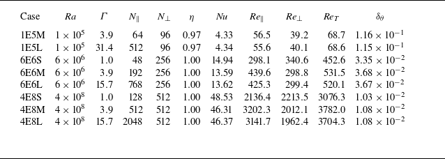
 Γ=L/H
 L
 H
 N‖
 N⊥
 η
 Re‖
 Re⊥
 ReT
 δθ

 1E5L
 6E6L
 4E8L
 1E5L
 Γ=31.4

 ∂⟨Θ⟩/∂z
 ⟨wθ⟩
 Rθ
 σRθ

 ⟨wθ⟩+
 κ
 ⟨wθ⟩
 λ+
 z+
 Ra=1×10⁵
 6×10⁶
 4×10⁸
 Γ
 δθ
 z+=z/δθ
 λ+=λ/δθ
 z∝λ

 z+
 ⟨wθ⟩
 κ
 EP,uwθ
 z+

 z+
 ⟨wθ⟩
 κ
 EP,θwθ
 z+

 z+
 ⟨wθ⟩
 κ
 ET⊥wθ
 Ra=1×10⁵
 6×10⁶
 4×10⁸
 Γ
 ET⊥wθ<0
 ET⊥wθ>0
 Fwθ(κ,z)=−∫0zET⊥wθdz′

 z+
 ⟨wθ⟩
 κ
 ET∥wθ
 Ra=1×10⁵
 6×10⁶
 4×10⁸
 Γ
 ET∥wθ<0
 ET∥wθ>0
 λ+
 z+
 Φwθ(κ,z)=−∫0κET‖wθdκ′

 z+
 ⟨wθ⟩
 κ
 EΠ,dwθ
 Ra=1×10⁵
 6×10⁶
 4×10⁸
 Γ
 EΠ,dwθ<0
 EΠ,dwθ>0

 z+
 RΠwθ=RΠ,dwθ+RΠ,swθ
 κ
 EΠwθ

 z+
 RDwθ
 ⟨wθ⟩
 κ
 EDwθ
 EDwθ
 Ra=1×10⁵
 6×10⁶
 4×10⁸
 Γ
 EDwθ<0
 EDwθ>0

 z+
 Rϵwθ
 ⟨wθ⟩
 κ
 Eϵwθ

 Open access

