





Food energy requirements (ERs) have been estimated by international and national committees for more than 50 years(1–6). The 1985 FAO/WHO/UNU report(5) introduced a factorial model of energy expenditure (EE) to predict energy requirements. This model has been utilised to a greater or lesser extent in all subsequent reports and specifically in the UK report on dietary reference values (DRV) in which the ER is assumed to match total daily energy expenditure (TEE), which in turn is predicted as basal energy expenditure (BEE) multiplied by the physical activity level (PAL) with PAL defined as TEE/BEE(3). Neufeld and Loechl, from FAO and the International Atomic Energy Agency (IAEA), respectively, recently indicated that it is time to update human ER(Reference Neufeld and Loechl7), based on their concerns about both gaps in the knowledge base and about previous methodologies used to determine ER and are jointly leading a new expert consultation begun in 2025. They have suggested that a predictive regression equation for total energy expenditure (TEE) derived from an IAEA database of doubly labelled water (DLW) studies of TEE can be used to estimate population ER from basic anthropometric and environmental data(Reference Bajunaid, Niu and Hambly8). This equation is derived with multivariant general linear regression modelling of a large database of DLW measurements for subjects aged 4 to 96 years held at the IAEA which is managed by a consortium who have contributed to the database(Reference Speakman, Pontzer and Rood9). The obvious advantage of a single prediction equation for all ages and both sexes is that it can potentially simplify the process of predicting TEE for specific age, size and sex groups, removing the need to identify the two main elements of the factorial model, that is, BEE, with prediction equations based on age, weight, height and sex, and categories of physical activity energy expenditure (PAEE) such as the PAL. Although a single prediction equation cannot account for variation in PAEE, which reflect behavioural phenotype and variable lifestyles, Neufeld and Loechl refer to reports of ecological DLW studies of TEE which failed to find that EE reflected active lifestyles, suggesting that physical activity is less important as a determinant of TEE than previously assumed(Reference Neufeld and Loechl7). However, further examination of these ecological studies of TEE has shown that when PAEE is correctly expressed as a simple function of body weight, TEE does reflect active lifestyles(Reference Millward, Betts and Bilzon10). Thus, PAEE will be an important determinant of TEE not accounted for in a prediction equation. According to Bajunaid(Reference Bajunaid, Niu and Hambly8), the prediction equation accounts for about 70 % of the variance in TEE which suggests that the unaccounted for 30 % could largely comprise unaccounted for PAEE. Furthermore, Bajunaid(Reference Bajunaid, Niu and Hambly8) did state that for athletes and individuals engaged in unusual levels of physical activity and for females during reproduction, all subjects with DLW-derived TEE in the IAEA database but not used in the derivation of the equation, their TEE was significantly underestimated by the prediction equation, and that the prediction equation cannot be used for these populations.
This is not the first prediction equation published from the IAEA DLW database by the consortium(Reference Pontzer, Yamada and Sagayama11), but that previous equation took as its inputs fat-free mass (FFM) and fat mass (FM), measures that may not be available when developing DRV for energy. Here, the intention is to first examine the performance of this prediction equation for 450 urban adults for whom DLW-derived TEE has been determined(Reference Subar, Kipnis and Troiano12,Reference Tooze, Schoeller and Subar13) and, second, to compare its performance against the factorial model adopted in deriving the UK DRV for energy for children and adults, as published by SACN(3), and an updated 2016 UK Government report on recommendations for ER(14).
Experimental methods
Ethical approval
All of this article derives from published material or as described below, information supplied to the author by the principal investigators of published studies. The author was not involved in the Observing Protein and Energy Nutrition Study (OPEN) study which was published with a full description of all ethical issues to do with the study subject selection, measurements made and data collection(Reference Subar, Kipnis and Troiano12,Reference Tooze, Schoeller and Subar13) .
Population groups tested
The first testing of the equation involved direct comparisons of its output against the OPEN study dataset of DLW-derived TEE which was originally obtained from Amy Subar (National Cancer Institute USA)(Reference Subar, Kipnis and Troiano12,Reference Tooze, Schoeller and Subar13) , during the preparation of the UK DRV(3), and is used here with the permission of Janet Tooze, an original principal investigator for the study. The dataset is very similar to another set of similar size and subjects, the Beltsville study(Reference Moshfegh, Rhodes and Baer15), reported around the same time with both sets combined and analysed together in the preparation of the UK 2011 SACN DRV report(3). Although the distribution of PAL values was very similar in each set, weight and heights were not reported in the Beltsville study, so it was not suitable for this analysis. While Dr Amy Subar, a principal investigator of the OPEN study, may at some stage have contributed DLW data to the IAEA database, she appears to have not contributed data to the dataset used to derive the equation because she is not listed among the eighty-nine authors identified as contributing to it in the report describing the prediction equation(Reference Bajunaid, Niu and Hambly8). It can be assumed therefore that the OPEN DLW data evaluated here was not used to derive the IAEA prediction equation.
The OPEN dataset was derived from DLW studies (n 450) involving healthy volunteers aged 40–69 years who were recruited from a random sample of 5000 households in the metropolitan area of Washington, DC (Montgomery County, MD, average elevation, 137 m). The cohort comprised 244 men and 206 women, who were 83 % Caucasian, 6 % African American, 5 % Asian, 4 % Hispanic and 2 %N/A. Most (87 %) had some college schooling with 63 % college graduates or postgraduates. The distribution by BMI groups was 31 % healthy (18·5 to <25 kg/m2), 41 % overweight (25 to < 30 kg/m2) and 29 % obese (≥30 kg/m2). Predicted TEE (pTEE) was calculated for all subjects by the equation. BEE was not measured but was estimated with Henry predictions which were based on sex, weight, height and age(Reference Henry16). These BEE values were used to factorise pTEE and derive predicted PAL (pPAL) values.
The second testing involved modelling the equations output against the various population groups for whom DRV for energy were derived by SACN(3) so that no real DLW data were used. Thus, the main purpose was to use the anthropometric data for children from 4 years of age, adolescents and adults to evaluate how the prediction equation works for this set of healthy body weights and heights, for which SACN modelled TEE to derive its DRV. SACN’s modelling involved the factorial method, which derived population DRV for energy as TEE = BEE × PAL as a function of age, height, weight and sex. BEE was calculated by the Henry equation(Reference Henry16) at ideal weights and actual heights reported for the population groups. PAL was derived as the median value for each DLW dataset used by SACN as a reference population for each age group. Clearly, it was not expected that pTEE would necessarily be the same as the TEE calculated by SACN modelling. The SACN DRVs were prescriptive, that is, derived for individuals at healthy body weights. Thus, at 4 years, the value for median weights and heights were derived from the WHO growth standards, while for children and adolescents aged 5–18 years they derived from the UK 1990 reference standards for children and adolescents and included lower body weights than those in the UK at the time of the report in 2011(3). Values for adult heights were for age bands for whom mean heights were reported in the Health Survey for England 2009(3). Weights were calculated as healthy weights, that is, at a BMI of 22·5 kg/m2, thus weight = 22·5 × height2. BEE was calculated from the Henry equations based on age, weight, height and sex(Reference Henry16). Because the Henry equations have overlapping age bands, (3–10 and 10–18 years), choice of equation is ambiguous at the age boundaries. SACN used the BEE equation for 4–10-year-olds for the 4–9-year-olds, and the equation for 10–18-year-olds was used for those aged 10–18 years on the basis of a smoother transition in the plot of BEE/kg against age. PAL values for children derived from a dataset of study means compiled from all then-published DLW studies of children aged over 1 year (170 data points as study means representing a total of 3502 individual measurements) (2082 females, 1420 males) (see SACN 2011, appendix 12 for details). No sex differences were identified for PAL values, and three age groups were identified within which the distribution of PAL values could be calculated: 1–3 years, >3–<10 years and 10–18 years. Median and 25th centile and 75th centile PAL values were identified for each of these groups, and the median values are used here having not been adjusted to account for the gross cost of energy deposition for growth. This means that the derived TEE values up to the age of 18 years can be directly compared with the pTEE. PAL values for adults are the median value for a dataset of 921 adult males and females assembled by SACN(3) trimmed for PAL values ≤1·27 or >2·5. This removed one subject with a PAL value >2·5 and thirty-eight subjects with PAL values <1·27, increasing the median PAL value from 1·62 to 1·63. pTEE was calculated for males and females at these ages, weights and heights living at an elevation of 70 m. pTEE was factorised to calculate pPAL with the same BEE values used by SACN.
In 2016, Public Health England published the Government Dietary Recommendations(14) which included revised values for energy for 11–18-year-olds and for 19–64-year-olds. These were capped at 10·5 MJ (2500 kcal)/d for males and 8·4 MJ (2000 kcal)/d for females (values which had at the time been in use by the food industry for some years as Guideline Daily Amounts), to help address issues of overweight and obesity in the UK. These values were compared with pTEE.
Finally, a stratified analysis of the equation’s performance with variation in BMI at two ages for each sex was performed with a comparison of the influence of BMI on TEE and PAL within the OPEN dataset.
Prediction equation
The IAEA DLW-based prediction equation tested here(Reference Bajunaid, Niu and Hambly8) predicts the natural logarithm of TEE.
That is,
ln (TEE) = −0·2172 +0·4167 × ln (BW) +0·006565 × Height −0·02054 × Age +0·0003308 Age2 −0·000001852 × Age3 +0·09126 × ln (Elevation) −0·04092 × Sex +0·01940 × A −0·03899 ×AA +0·006238 × AS +0·02626 × W −0·0155 × H +0·003589 × NA −0·0006759 × Height × ln (Elevation) +0·002018 × Age × ln (Elevation) −0·00002262 × Age2 × ln (Elevation) − 0·006947 × Sex × ln(Elevation). For the self-reported ethnicity codes, for African, A was 1 and 0 otherwise, for African individuals living outside Africa, AA was 1 and 0 otherwise, for Asian, AS was 1 and 0 otherwise, for White, W was 1 and 0 otherwise, for Hispanic, H was 1 and 0 otherwise, and for not available, NA was 1 and 0 otherwise. Mixed race individuals were coded as NA.
Calculations
Spreadsheets were created containing the detailed anthropometry, ethnicity and DLW-derived TEE for the OPEN cohort, and the SACN-derived data, which included anthropometry, calculated BEE, PAL values and calculated TEE for all ages from 4 to 75+ years, along with similar data relating to the Government Dietary Recommendations for Energy(14). These spreadsheets were modified to contain the variables within the prediction equation so that predicted lnTEE could be calculated by the formula above. To check that it was correctly set up, the variables described in the two published worked examples(Reference Bajunaid, Niu and Hambly8), an Asian female living in Aberdeen and a Hispanic man living in Boston, USA, were added to the spreadsheet so that their TEE could be predicted in the same way as all other subjects. The computed values for lnTEE for these two subjects were identical to their published values indicating that the equation had been correctly entered into the spreadsheet. The upper and lower 95 % predictive intervals were calculated with the reported equations(Reference Bajunaid, Niu and Hambly8), that is, lower 95 % PI = (pTEE × 0·7466) − 1·5405 MJ/d, upper 95 % PI = (pTEE × 1·3395) + 2·7668 MJ/d. Values were calculated for each predicted pTEE value, and the linear regression lines were calculated for all subjects.
Statistical analysis
Graphical comparisons of predicted and measured TEE incorporating linear regression were performed to decide what comparisons were appropriate. Because it became apparent that the sex term in the equation resulted in some unexpected differences in its performance, all analysis was done separately for males and females. Analysis mainly used Excel and IBM SPSS Statistics, version 32.0.0.0 (134), made available by IBM in April 2026. Bland–Altman plots with limits of agreement and assessment of proportional bias were performed. The prediction error was evaluated in terms of mean absolute error, root mean square of error (RMSE) or absolute percentage error and Lin’s concordance correlation coefficient (CCC).
Elevation above sea level is a factor in the equation on its own and as interactive terms with height, age and sex. To evaluate the influence of elevation, TEE was predicted for two individual OPEN subjects, that is, a 52-year-old male of 54 kg and 172 cm height and a 41-year-old female of 45·2 kg and 150 cm height, at nine elevations ranging from 10 to 4000 m.
Results
In the two worked examples reported by Bajunaid et al.,(Reference Bajunaid, Niu and Hambly8) a Hispanic male living in Boston, USA (elevation 14 m), and an Asian female, living in Aberdeen UK (elevation 39 m), 1·51 m tall, 22 years old, weight 46·5 kg, the equation predicted TEE values of 12·2 MJ/d and 8·05 MJ/d. These were equivalent to PAL values of 1·60 and 1·71, after factorisation with BEE values, calculated from sex, heights, weights and age with the Henry equations(Reference Henry16).
The ethnicity factors had small relative effects in that compared with the pTEE for White Caucasians (the largest ethnicity regression coefficient), all other ethnicity factors lowered TEE by between 0·7 % for Africans and 6·3 % for African Americans.
Testing on the OPEN dataset
Table 1 shows the reported and predicted mean values of TEE for the OPEN dataset for all subjects and for males and females separately. Also shown are reported and predicted derived values for measures of physical activity energy expenditure as PAEE, PAL and the more sensitive indicators, PAEE/BEE and PAEE/weight (see Millward et al.(Reference Millward, Betts and Bilzon10)), calculated with the same predicted BEE in each case.
Reported and predicted energy expenditure for the OPEN cohort

Table 1 Long description
Table listing both reported and predicted mean, SD, median, minimum and maximum values for TEE, PAEE, PAL, PAEE/BEE and PAEE/weight for subjects in the OPEN cohort shown for the total cohort (n 450) males(n 244) and females (n 206)
TEE, total energy expenditure; PAEE, physical activity energy expenditure; PAL, physical activity level; BEE, basal energy expenditure; pTEE, predicted TEE; pPAEE, predicted PAEE; pPAL, predicted PAL.
* Calculated as 0.9×TEE-BEE predicted by the Henry equation(Reference Henry16).
† TEE/BEE with BEE predicted by the Henry equation(Reference Henry16).
The reported OPEN data values show a wide range of TEE, reflecting a wide range of both BMI (mean 27·9, range 17·4–51 kg/m2) and PAL values. PAL and derived variables of physical activity were not normally distributed, that is, slightly skewed towards the inactive subjects, so that median values for TEE and derived variables were all slightly lower than mean values. Males exhibited higher values for TEE than females but on average slightly lower values for PAL and adjusted PAEE than females.
For the predicted values, pTEE and derived PA variables, values were normally distributed with similar mean and median values for pPAEE, pPAL and its derived values. The overall mean pTEE value was slightly underpredicted, by 0·27 MJ/d, mainly because females were underpredicted (0·44 MJ) with lower pPAEE, pPAL and derived values. The reason for this sex difference in the mean bias appeared to be that the equation predicted slightly higher values for pPAL and its derived variables, for males compared with females, although actual reported values were slightly higher in females than in males. However, the most obvious difference between reported and predicted values shown in Table 1 was that for the predicted values, there was a much lower range of variation in the values for pTEE and the physical activity measures as indicated by the lower sd values and overall range. An examination of the relationships between bias and major predictors such as weight indicated that it was quite random.
Figure 1 shows how well the prediction equation performs on an individual basis in this dataset. Regressions of predicted values on measured TEE for males and females are shown which can be compared with the line of equality.
Performance of prediction equation. pTEE calculated by the IAEA equation reported by ref. 8 is compared with measured values reported for the OPEN cohort(Reference Tooze, Schoeller and Subar13) with males and females shown separately and with the line of equality also shown. The upper and lower 95 % predictive intervals, (PI), are shown as calculated with the equations reported by Bajunaid et al., 2025. That is, lower 95 % PI = (pTEE × 0.7466) −1.5405 MJ/d and upper 95 % PI = (pTEE × 1.3395) +2.7668 MJ/d. Values were calculated for each predicted value (pTEE), and the linear regression lines are shown calculated for all subjects. The 95 % prediction intervals calculated in this way are quite wide, and all subjects fall within the 95 % PI regression lines. The regression equations are as follows: males: predicted TEE = 0.355 × measured TEE + 7.66 MJ/d: R 2 = 0.44; females: predicted TEE = 0.414 × measured TEE + 5.21 MJ/d: R² = 0.45. The large positive intercepts and shallow slopes indicate that much of the variance in measured TEE is unaccounted for in the prediction equation, that is, R 2 values <0.5. Also these shallow slopes and a comparison of predicted values with the line of equality indicate that the equation shows heteroscedasticity, that is, overprediction at low values and underprediction at high values of TEE. The CCC, which evaluates both precision (correlation) and accuracy (deviation from the 45-degree identity line), indicated poor agreement between measured and predicted TEE (CCC = 0.622) (males) and 0.648 (females). pTEE, predicted total energy expenditure; IAEA, International Atomic Energy Agency; OPEN, Observing Protein and Energy Nutrition Study; PI, prediction interval; CCC, concordance correlation coefficient.

Figure 1 Long description
> X-Y plot of individual values of predicted TEE as a function of measured TEE in MJ/d shown separately for males and females with lines for linear regressions, the line of equality and lines showing upper and lower 95% prediction intervals.
The upper and lower 95 % predictive intervals are also shown as calculated with the equations reported by Bajunaid et al.(Reference Bajunaid, Niu and Hambly8). There are large positive intercepts and shallow slopes for the regression lines, and their equations show that much of the variance in measured TEE is unaccounted for in the prediction equation (low R 2 values). Thus, the variation in the accuracy of the predicted values of TEE was such that only 44–45 % of the variance in the measured TEE was explained. The greater intercepts for men (7·7 MJ) compared with women (5·2 MJ) indicated a larger absolute error for men than women (although reported TEE was as expected larger for males). When values are compared with the line of equality, it is clear that the equation shows heteroscedasticity with overprediction at low values and underprediction at high values of TEE. While all predicted values fit within the 95 % PI, these intervals are quite wide as calculated. As would be expected from the equations’ heteroscedasticity, indicated by the deviation from the line of equality, the CCC indicated poor agreement between measured and pTEE (CCC = 0·613) (males) and 0·652 (females). The CCC evaluates both precision (correlation) and accuracy (deviation from the 45-degree identity line), and whilst opinions differ on the interpretation of CCC values, some suggest values below 0·9 represent poor agreement.
Bland–Altman plots of predicted–measured TEE against measured TEE together with mean differences and 95 % agreement limits are shown in Figure 2. The differences between TEEp and TEEE varied over a wide range for each sex from positive at low TEE values to negative at high TEE values due to overprediction at low values and underprediction at high values of TEE, indicating proportional bias which as would be expected was highly significant at p < 0·001 in each case. Mean differences or mean absolute errors with 95 % CI were −0·140 MJ/d (−0·351 to 0·071 MJ/d males) and −0·435 MJ/d (−0·602 to −0·269 MJ/d females), with 95 % agreement limits from −3·42 MJ/d to 3·14 MJ/d (males) and −2·82 MJ/d to 1·95 MJ/d (females).
Bland–Altman plot of measured and predicted TEE. The Bland–Altman plot of predicted–measured TEE showed that values varied over a wide range for males and females but because of the heteroscedasticity of the prediction equation, predicted–measured TEE values were for each sex, positive at low TEE values and negative at high TEE values due to overprediction at low values and underprediction at high values of TEE. Mean differences or mean absolute errors (solid lines) with 95 % CI were −0.140 MJ/d (−0.351 to 0.071 MJ/d males) and −0.435 MJ/d (−0.602 to −0.269 MJ/d females) and 95 % agreement limits (dotted lines) were from −3.42 MJ/d to 3.14 MJ/d (males) and −2.82 MJ/d to 1.95 MJ/d (females). Analysis of proportional bias showed that as would be expected, it was highly significant (p < 0.001) for each sex. TEE, total energy expenditure.

Figure 2 Long description
X-Y plot of individual values of predicted - measured TEE as a function of measured TEE in MJ/d shown separately for males and females with lines showing the mean difference and the 95% agreement limits.
The magnitude of the errors as a percentage is shown in Figure 3 in which the accuracy of pTEE is shown as a function of the measured TEE. The mean absolute percentage errors were −1·2 (males) and −4·5 (females). The RMSE and %RMSE were 1·67 MJ/d (14·3 %) (males) and 1·29 (8·82 %) MJ/d (females). As shown in Figure 1, the overprediction in those with below-average TEE and underprediction when TEE was above average are clear. Predictions are often deemed as accurate when the % error ≤± 10 %(Reference Prado-Nóvoa, Howard and Laskaridou17). Although the range of errors was large, >±35 %, just over half of the predicted values (54 %) were within ≤±10 %. Of the inaccurate predictions (those with errors outside the ±10 % range), the overpredictions up to 40 %(M) and 31 %(F) amounted to absolute average values of 1·7 MJ/d (M) and 0·9 MJ/d (F), while the underpredictions up to −35 % (M) and −32 % (F) amounted to −3·1 MJ/d (M) and −1·9 MJ/d (F).
Accuracy of predicted TEE as a function of the measured TEE. The mean absolute percentage errors were −1.2 (males) and −4.5 (females). Predictions are often deemed as accurate when the % error <±10 %(Reference Prado-Nóvoa, Howard and Laskaridou17). The root mean square of error (RMSE) and %RMSE were 1.67 (14.3 %) and 1.29 (8.8 %) MJ/d for males and females, respectively. Although the range of errors was large, >±30 % about half of the predicted values (56 % (M) and 53 % (F)) were within ≤± 10 % and deemed to be accurate. Of the inaccurate predictions, the underpredictions amounted to on average −3.1 MJ/d (M) and −1.9 MJ/d (F) and the overpredictions amounted to on average 1.7 MJ/d (M) and 0.9 MJ/d (F). TEE, total energy expenditure.

Figure 3 Long description
> X-Y plot of individual values of the % error of predicted TEE as a function of measured TEE in MJ/d shown separately for males and females, with accurate values (those with errors ≤10%) highlighted within +10 to −10 % boundaries.
The extent to which interindividual variation in PAEE, which is not accounted for in the prediction equation, accounts for the heteroscedasticity of its bias in predicting TEE is shown in Figure 4. PAEE is shown as PAEE/BEE, a metric which is independent of body weight and a more sensitive exact measure of PAL(Reference Millward, Betts and Bilzon10). Physical activity within the test population group is clearly a determinant of most of the bias in the prediction equation explaining 92–93 % of its variation. Whilst this means that the prediction is accurate (±10 %) for those near the centre of the distribution of PAEE, for the less active or more active remainder, it will either over-or underpredict by considerable amounts. Calculations of bias indicates that for subjects classified by PAEE/BEE, average bias for Q1 (least active) and for Q4 (most active) was for males 2·11 and −1·69 MJ/d and for females 1·27 and −1·65 MJ/d for these two quartiles. The sex difference in assigning PAEE and PAL values is shown as the PAEE/BEE and PAL values at zero bias: that is, for males: PAEE/BEE = 0·45 (PAL = 1·60) and females: PAEE/BEE = 0·43 (PAL = 1·59). It must be noted that because both bias and PAEE are derived from measured TEE, part of the very high R² values observed between bias and PAEE/BEE may result from mathematical coupling rather than reflecting only the true contribution of physical activity to the prediction error.
Physical activity as a determinant of most of the bias in the prediction equation. Interindividual variation in PAEE cannot be accounted for in the IAEA prediction equation and most likely accounts for the heteroscedasticity of its bias in predicting TEE. Variation in PAEE which is independent of body weight can be expressed as PAEE/BEE a more sensitive exact measure of PAL(Reference Millward, Betts and Bilzon10). The regressions shown here for men and women clearly show that variation in PAEE/BEE explains most (92–93 %) of the bias (predicted–measured TEE) of the IAEE prediction equation. Thus, the prediction is accurate (±10 %) for those in the middle of the distribution of PAEE but for those in the bottom or top quartiles of PAEE, it will over-or underpredict by considerable amounts. The regression equations are males: bias (MJ/d) = –8.5 PAEE/BEE + 3.8 R² = 0.92; females: bias (MJ/d) = –6.1 PAEE/BEE + 2.61 R² = 0.93. For zero bias (M): PAEE/BEE = 0.45 (PAL = 1.60) (F): PAEE/BEE = 0.43 (PAL = 1.59). PAEE, physical activity energy expenditure; IAEA, International Atomic Energy Agency; TEE, total energy expenditure; BEE, basal energy expenditure; PAL, physical activity level.

Figure 4 Long description
X-Y plot of individual values of the Bias of predicted TEE values, as MJ/d, as a function of measured PAEE/BEE shown separately for males and females with linear regressions lines shown.
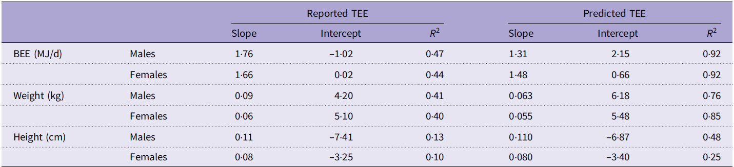
These results suggest that the IAEA prediction equation predicts mainly the BEE of the subjects together with an additional amount of EE representing average PAEE which is what might reasonably be expected given the input variables based on anthropometric and environmental factors. BEE was not measured in the OPEN cohort but was derived from the Henry equations, and Table 2 shows BEE, weight and height as predictors of TEE in the evaluation cohort and in the pTEE tested by linear regression. For the measured TEE, BEE and its predictors, weight and height accounted for a maximum of 47 % of the variance in TEE, with presumably the rest of the variance being attributable to the variable amount of PAEE. However, for the pTEE because none of the predictors in the equation would be expected to account for actual PAEE, much larger proportions of the variance was accounted for by BEE and its predictors, weights and height. (It should be noted that, although in deriving the prediction equation the authors argued that the most significant predictor of TEE was the natural logarithm of body weight, there was no difference in the R 2 values for regressions of ln weight and weight against observed or pTEE for the OPEN dataset examined here).
BEE as a predictor of TEE and influence of weight and height as predictors in the evaluation cohort and in the predicted TEE tested by linear regression

Table 2 Long description
Table showing the slope, intercepts and R2 values for BEE, weight and height as predictors of both reported and predicted TEE for males and females.
BEE, basal energy expenditure; TEE, total energy expenditure.
Figure 5 shows graphically how BEE explains 92% (M&F) of the variance of pTEE. For females, the slope (1·48) is closer to the mean PAL value calculated from the pTEE (1·59 see Table 1) because the intercept is small (i.e. less of the unaccounted-for PAEE is associated with the intercept). However, for males, the prediction equation works a little differently in that the slope (1·32) of pTEE on BEE is much less than the pPAL value (1·61) because the intercept is significant at 2·15 MJ/d, implying that more of the unaccounted-for PAEE is associated with the intercept.
Predicted TEE as a function of the BEE. BEE was not measured but was derived from the Henry equations. Regression of pTEE on BEE shows that BEE explains 92% of the variance in pTEE (M&F). For males, the slope (1.32) is less than the mean PAL value (1.61) because the intercept is significant at 2.15 MJ/d. However, for females the slope (1.48) is closer to the mean PAL value (TEE/BEE, 1.59) with the intercept smaller. The regression equations are as follows: males (n 244): predicted TEE (MJ/d) = 1.32 × BEE + 2.15 R² = 0.92; females (n 206): predicted TEE (MJ/d) = 1.48 × BEE + 0.66 R² = 0.92. TEE, total energy expenditure; BEE, basal energy expenditure; pTEE, predicted total energy expenditure; PAL, physical activity level.

Figure 5 Long description
X-Y plot of individual values of predicted TEE values, as MJ/d, as a function of predicted BEE as MJ/d shown separately for males and females with linear regressions lines shown.
To further examine to what extent the equation predicted any PAEE, the way in which the pPAL value (pTEE/BEE) varied with anthropometric predictors within the equation was calculated by linear regression of pPAL against weight, height and age. There were no obvious relationships with age or height in men or women (R 2 values<5 %), but there was a significant inverse relationship with weight in men (pPAL = −0·0021 weight + 1·79 R² = 0·37) but no relationship in women.
Thus, for men, pPAL was highest in those with body weights or BMI values considered healthy, falling markedly with overweight or obesity, relationships that were also significant in females but less marked, with lower overall pPAL vales. This was in contrast to the measured PAL which was not related to weight or BMI. Modelling the effect of increasing BMI at fixed heights is shown in Table 4 and discussed below. The effects of these sex differences in the way the equations works is also discussed further below.
Influence of elevation on predicted TEE
In the prediction equation examined here, elevation in metres is included as its natural logarithm both on its own and as interactive terms with height, age, age2 and sex. To test its influence, TEE was calculated by the equation for individual male and female OPEN adults, at 10 elevations ranging from 1 to 4000 m. The results are shown in Figure 6. Because of the logarithmic relationship between elevation and TEE in the prediction equation, TEE increased markedly with initial increases in elevation, for example, by 12·7 % at 100 m and almost 20 % at 1000 m but increasing much less markedly after that, so that at 4000 m TEE was 24 % higher than at sea level (1 m). At the assumed elevation for the OPEN subjects (137 m), TEE was 13·7 % higher than at sea level (1 m).
Predicted TEE as a function of elevation above sea level (m). Values are calculated for two individual OPEN subjects, a 52-year-old male of 54 kg and 172 cm height and a 41-year-old female of 45.2 kg and 150 cm height, at ten elevations ranging from 1 to 4000 m. Values fit equations are as follows: males: TEE (MJ/d) = 0.2634 ln(elevation(m)) + 9.0655 R² = 0.999; females: TEE (MJ/d) = 0.2142 ln(elevation (m)) + 6.84: R² = 0.9989. TEE, total energy expenditure; OPEN, Observing Protein and Energy Nutrition Study.

Figure 6 Long description
X-Y plot of predicted values for TEE as a function of elevation above sea level in meters calculated for an individual male and female identified from the OPEN cohort.
Testing against the SACN population of healthy weights and heights for all ages 4–75+years
pTEE calculated for males and females at the healthy weights and heights used by SACN from the age of 4 to 80 years is shown in Figure 7a, and TEE/kg body weight, the intensity of EE, is shown in Figure 7b, with details in Table 3 of the calculated values compared with values for TEE as reported by SACN(3), which was predicted from BEE and PAL by the factorial model from the age of 4 to 80 years. For the prediction equation, given the smooth age-related changes in weights and heights shown in Table 3, Figure 7a shows, as would be expected, a smooth age-related change in pTEE which increased to a peak in males at 22 years and 17 years in females and then declined gradually and more steeply after 70 years. Similarly, pTEE/kg (Figure 7b) fell smoothly for males and females throughout childhood and adolescence up to early adulthood, declining slowly and uniformly up to 60 years and more steeply after that.
Predicted TEE values at healthy weights and as TEE/kg body weight from 4 to 80 years of age. Values shown are for males and females from values calculated from the prediction equation(Reference Bajunaid, Niu and Hambly8) at healthy body weights reported by SACN(3) expressed as: (a)TEE/d (MJ/d) and (b)TEE/kg body weight (MJ/d/kg). TEE, total energy expenditure.

Figure 7 Long description
X-Y plot of predicted values for TEE as a function of healthy body weights from 4 to 80 years of age for males and females expressed as: a)TEE/d (MJ/d) and b)TEE/kg body weight (MJ/d/kg).
Equation testing against SACN TEE values

Table 3 Long description
Table showing weights, heights, BEE, PAL, and TEE values reported by SACN together with predicted values for TEE and PAL and the difference between reported and predicted TEE values as MJ/d and as a %age for males and females at ages from 4 to 80 years.
TEE, total energy expenditure; BEE, basal energy expenditure; PAL, physical activity level; pTEE, predicted TEE; pPAL, predicted PAL.
* For children and adolescents, median weights and heights derive from the WHO growth standards (ages 4 years) and the UK 1990 reference for children and adolescents for children aged 5–18 years(3). Values for adult heights are shown for age bands for whom derived mean heights were reported in the Health Survey for England 2009(3). The individual ages from 22 to 80 years were used for the pTEE. Adult weights are calculated as healthy weights (at BMI = 22.5 kg/m2), that is, weight = 22.5 × height2.
† Calculated from the Henry equations based on weight and height(Reference Henry16). Because the Henry equations have overlapping age bands (0–3, 3–10, 10–18 years), choice of equation is ambiguous at the age boundaries. Here, the BEE equation for 4–10-year-olds is used for the 4–9-year-olds and the equation for 10–18-year-olds is used for those aged 10–18 years on the basis of a smoother transition in the plot of BEE/kg against age.
‡ PAL values for children are the median of all reference study means for subjects aged 4–9 and 10–18 years, not adjusted to account for the cost of energy deposition for growth. PAL values for adults are the median values for a dataset of 921 adult males and females assembled by SACN(3) trimmed for PAL values ≤1.27 or >2.5. This removed one subject with a PAL value >2.5 and thirty-eight subjects with PAL values <1.27 increasing the median PAL value from 1.62 to 1.63.
§ Calculated as BEE × PAL.
¶ Calculated from the prediction equation reported by Bajunaid et al.(Reference Bajunaid, Niu and Hambly8) assuming all subjects were White Caucasian living at an average elevation of 70 m.
‖ Calculated as pTEE/BEE.
** Difference between predicted and SACN values for TEE as MJ/d and as a percentage.
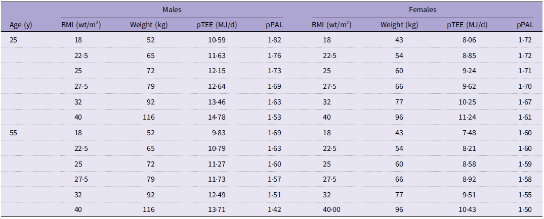
Modelling the influence of BMI on pTEE and pPAL *

Table 4 Long description
Table showing BMI, weights, predicted TEE and predicted PAL values for males and females at increasing BMI values from 18 to 40kg/m2 calculated for individuals at the separate ages of 25 and 55 years of age.
pTEE, predicted total energy expenditure; pPAL, predicted physical activity level.
* Values were calculated at heights of 170 cm (males) and 155 cm females at each indicated age.
The modelling adopted by SACN resulted in a somewhat different pattern of age-related changes in TEE (see Table 3) with discontinuities between 9 and 10 years and between 18 and 22 years which were age boundaries for changes in both the BEE predictive equation and in chosen PAL values. Thus, adolescents were assumed to be more active (PAL = 1·73) than either children <10 years (PAL = 1·57) or adults (PAL = 1·63). Because the modelling assumed no sex differences in PAL, the sex differences in TEE only reflected different predicted BEE values. The consequence of this modelling was differences between pTEE and TEE shown in Table 3 as absolute MJ/d and %age values, which reflected both age and sex.
For males, these differences meant that the equation slightly overpredicted TEE up to the age of 9 years (by 4·2 % maximum) but underpredicted from 10 years up to the age of 18 years by −4·8 % maximum. After this, all adult values up to the age of 70 years are overpredicted, initially by 9·1 %. In the eldest age band (80 years), the equation predicted 2·9 % lower TEE than the SACN value because SACN prescribed TEE for active elderly subjects with the same PAL as for younger adults.
For females, there was a different pattern of differences in that the equation underpredicted for all children and adolescents up to 18 years of age by various amounts from 3·5 to 9·2 % and then mainly overpredicted for adults between 22 and 40 years of age after which values were not very different until 80 years of age when, as with the males, a reduction in TEE was predicted.
Examination of the pPAL values from the factorised pTEE (Table 3) indicates a complex age-related pattern of changes reflecting the age boundaries of the BEE prediction equation and shows an obvious sex difference for all ages. For young children, pPAL values were markedly lower in females than males, and this difference persisted during adolescence after the abrupt changes at 11 reflecting changes in predicted BEE by the Henry BEE prediction equations. However, pPAL values for males and females converged at 18 years but after the abrupt increase at 22 years due to the change to a lower predicted BEE, the sex differences remained with lower values for females as the slow decline in pPAL with age continued.
Figure 8 shows pTEE and the UK current ER values as MJ/d for males and females from 5 to 80 years of age. Values shown are derived from the 2016 UK Government Dietary Recommendations for Energy(14) which include values for age bands 4–6, 7–10, 11–14, 15–18, 19–64, 65–74 and 75+ years, with values derived from the 2011 SACN report(3) but capped (at 2500 kcal/d, 10·5 MJ/d males and 2000 kcal/d, 8·4 MJ/d females) between 11 and 64 years because of concern for overweight and obesity. To enable comparable pTEE values to be calculated by the prediction equation, values shown are at ages 4, 8·5, 12·5, 16·5, 19, 22, 64, 70 and 80 years with weights and heights shown or interpolated from Table 3. This resulted in marked differences between pTEE and all the capped ER values for adolescents, with the maximum values for pTEE being 20 % greater at 22 years for males and 16 % greater for females at 19 years of age.
pTEE and UK current energy requirement values (MJ/d) for males and females from 5 to 80 years of age. Values shown derive from the 2016 UK Government Dietary Recommendations for Energy(14) which include values for age bands 4–6, 7–10,11–14,15–18,19–64 65–74 and 75+ years, with values derived from the 2011 SACN report capped between 11 and 64 years because of concern for overweight and obesity. To enable comparable pTEE values to be calculated by the prediction equation, values shown are at ages 4, 8.5, 12.5, 16.5, 19, 22, 64, 70 and 80 years with weights and heights shown or interpolated from Table 3. pTEE, predicted total energy expenditure.

Figure 8 Long description
X-Y plot of both predicted values for TEE and the UK current energy requirements (MJ/d) for males and females as a function of healthy body weights from 4 to 80 years of age.
Finally, the effect of increasing BMI at fixed heights and at two ages is shown in Table 4 for male and females. This showed that for subjects aged 25 years with BMI values from 18 to 40 kg/m2, TEE increased by 39 % for males and females, with pPAL values falling more in males from 1·82 to 1·53 (16 %) than in females from 1·72 to 1·61 (6·4 %). For older subjects at 55 years, while pTEE and pPAL values were lower, as expected by the age-related changes in Figure 7, with increasing BMI, the same proportional changes in pTEE and pPAL occurred. Thus, at 25 and 55 y, with increasing BMI, the PAEE component of the TEE is predicted to fall more in males than in females. This influence of BMI on pTEE in adults was different from that observed within the OPEN population within which, although TEE tended to increase with BMI, BMI explained only about 30 % of the variance of TEE for males and females because there was no significant relationship between BMI and PAL in either sex.
Discussion
Many attempts to predict TEE from weight, height and other variables have been published, and nine prediction equations were recently evaluated in a group of subjects in which TEE was measured by DLW, three of which included measured PAEE(Reference Prado-Nóvoa, Howard and Laskaridou17). Although all of these equations were derived to some extent from DLW data, all underestimated TEE and none met all criteria to be considered accurate. Bias increased with increasing physical activity with all equations. Notably, the three equations which included measured activity did not improve bias. The authors devised a prediction equation for TEE based on their own use of a triaxial accelerometer (ActiGraph GT3X) to measure PAEE, together with measured BEE and the predicted thermic effect of food, and this equation was described as no better than any other.
Prediction equations derived by general linear regression modelling describe the relationships which exist between measured values within the datasets. According to Bajunaid et al.(Reference Bajunaid, Niu and Hambly8), the prediction equation, used here, derived from 7441 individual DLW measurements of TEE from a larger database collected from thirty-two countries. These were healthy male and female individuals aged 4 to 96 years, not engaged in dietary or exercise interventions or in unusual levels of physical activity and were not pregnant or lactating females. They did include measurements of hunter–gatherer and subsistence agriculture populations who have higher than average values for PAEE/BEE and PAEE/weight(Reference Millward, Betts and Bilzon10), but these accounted for <1 % of the total measurements. The authors identified a randomly derived 90 % (n 5899) of the qualifying measurements to derive the prediction equation, and this was tested against the other randomly derived 10 % (n 598). 95% PIs were also calculated from the estimated mean and the standard error of the regression coefficients indicated by the regression modelling, by standard methods allowing the equations used here (see Figure 1) to define the upper and lower 95 % PI for pTEE. 94·6 % of the authors’ test population’s pTEE measurements were within these 95 % PIs, although they were quite wide. The overall equation for pTEE based on general linear modelling explained about 69 % of the variation in TEE in the test population.
Theoretically, any prediction equation derived from the modelling of measured TEE against anthropometric and environmental factors will identify significant relationships between TEE and those variables on which EE depends. Physiologically, a major part of EE comprises BEE which varies with body size and composition, mainly the FFM, and is predictable from height, weight, age and sex. The rest of EE, PAEE and any other thermogenesis will vary independently from these factors. Although these components of TEE cannot be predicted on an individual basis, it is to be expected that during general linear regression modelling, the non-BEE part of pTEE will be included in pTEE as the average PAEE of the population from which the equation is derived. The modelling process will distribute this average PAEE between the constant in the equation and the coefficients of the equation variables in a way that is difficult to predict, especially with the large number of variables and their interaction in the Bajunaid et al(Reference Bajunaid, Niu and Hambly8) equation shown above. Nevertheless for a population with a similar average PAL value as those subjects in the IAEA DLW database, the equation should predict similar overall levels of TEE with reasonable accuracy. However, it should under-or overpredict for those more or less active than assumed by the prediction equation in the same way that was observed by Prado‑Nóvoa et al.(Reference Prado-Nóvoa, Howard and Laskaridou17) in their testing of TEE prediction equations described above.
The testing of the TEE prediction equation described here involves limitations which must be recognised at the outset, the main one being the factorisation of both the measured TEE and pTEE values with predicted values of BEE. The value of such factorisation of pTEE is that it allows to some extent the way in which the prediction equation works to be examined, that is, how much PAEE is included in the pTEE. However, BEE values are associated with errors, and such factorisation may be unacceptable to critics of the factorial model(Reference Speakman and Pontzer18). Whilst there are many BEE prediction equations each associated with a level of uncertainty, SACN identified the Henry equations(Reference Henry16) on the basis of a detailed examination of the issue (see Appendix 4(3)). A more recent evaluation of the performance of the Henry prediction equations also identified it as the most valid out of eight others for predicting REE in adult males and females(Reference Fernández-Verdejo and Galgani28). In any case, it is unlikely that the very obvious relationships between bias and PAEE/BEE (Figure 4), pTEE and BEE (Figure 5), and the arguments about pPAL values in Table 3, which depend on factorisation of either measured TEE or pTEE, would be substantially changed with a different BEE prediction equation. The factorisation of TEE is discussed further below in the strengths and limitations section.
The testing of the prediction equation described here against the OPEN adult urban population reveals its performance on an individual basis and broadly reflects theoretical predictions. As described above under population groups tested, SACN identified this population group as sufficiently similar to the UK adult population to serve as a reference (together with another very similar large cohort(Reference Moshfegh, Rhodes and Baer15)) from which to derive the UK population DRV. As can be seen in Figure 1, each pTEE value was within the 95 % PI based on the authors’ equations, although the range of these PI was quite large. The average pTEE was only 0·28 MJ underpredicted (Table 1), and assessment of individual accuracy as ≤±10 % showed that the equation was accurate for about half of the predicted values (54 % M and F). However, as expected, it under-or overpredicted for those who were more or less active than the median by >±35 % (Figure 3).
Factorisation of pTEE to give pPAL and the more sensitive measures of PAEE allowed insight into how the equation distributed PAEE between the prediction variables within the OPEN population. Males, who were on average underpredicted (−0·14 MJ), compared with an underprediction for females of −0·44 MJ, exhibited a similar overall % accuracy to females yet exhibited pPAL values and its derived variables which were slightly higher than for females. This was also observed for the SACN cohort, with more substantial sex differences for young children and adults (see Table 3). In deriving its factorial model for the UK DRV, SACN did not identify any sex difference in PAL values in DLW studies for the dataset of 950 adults of which the OPEN population examined here comprised half or in the dataset used to identify the DRV of children or adolescents. This was a large dataset of 1701 studies with 3502 individual measurements (females = 2082, males = 1420). In fact as shown in Table 1, reported PAL values for the OPEN cohort were slightly higher in females than in males. It is not known how many of the values assembled by SACN for children and adults are included in the IAEA DLW database from which the prediction equation was derived.
The OPEN testing showed that for both males and females, as might be expected, most of the variance in pTEE (90–95 %) is associated with those factors which predict BEE (see Table 2). However, for females, the slope of the regression of BEE on TEE (1·48) is closer to the mean pPAL value (1·59: see Table 1 and Figure 5). Because the intercept for this regression is relatively small (0·66 MJ/d), this means that for females, the prediction equation, in practice, assigns a major component of PAEE as a fixed fraction (0·48) of the BEE. For males, the regression of BEE on pTEE is somewhat different with a shallower slope (1·32) and a larger intercept. This means that, effectively, PAEE is assigned as a lower fixed fraction of BEE (0·32) plus a greater fixed absolute amount (2·15 MJ/d), which equates to about 80 % of the estimated PAEE shown in Table 1. In practice, these two slightly different allocations of PAEE for males and females did not affect the accuracy of the equation. However, the use of the equation to derive ER values will result in a greater difference between male and females than currently identified by factorial models in which sex influences TEE only through the BEE component.
The influence of elevation within the equation is a somewhat surprising feature. Environmental elevation above sea level has not been a consideration in relation to energy balance in international reports on ER to date, yet approximately 140 million people are reported to live above 2500 m(Reference Murray19), with about 5 million people living on the Tibetan Plateau at an average of 4000 m(Reference Price20). Whilst adaptive changes to the lower oxygen tension are known(Reference Yang, Jin and Chen21), exactly how this influences energy balance is poorly understood. Phala Nomads living at 4850–5450 m on the northern plateau of Tibet exhibit BEE values measured at thermoneutrality which for males were similar to predicted values and only very slightly higher for females(Reference Beall, Henry and Worthman22). The Aymara agropastoralists from the Bolivian altiplano who live at an approximate elevation of 4000 m above sea level are reported to exhibit BEE values slightly lower (5·6 %) than predicted by the Schofield equations(Reference Kashiwazaki, Dejima and Orias-Rivera23) but exhibit very high rates of TEE(Reference Kashiwazaki, Dejima and Orias-Rivera23,Reference Kashiwazaki, Uenishi and Kobayashi24) comparable to the highest levels observed in Western urban societies and similar to values within the UK military when compared on the basis of weight-adjusted PAEE(Reference Millward, Betts and Bilzon10). Because of the logarithmic relationship between elevation and TEE in the prediction equation, Figure 6 shows that TEE increased markedly with elevation at low elevations but increased much less markedly after that. Thus at 4000 m, TEE was 24 % higher than at sea level (1 m) compared with 12·7 % at 100 m. At the assumed elevation for the OPEN subjects (137 m), TEE was predicted to be 13·7 % higher than at sea level (1 m). Bajunaid et al.(Reference Bajunaid, Niu and Hambly8) report that in their regression modelling, the effects of elevation were unanticipated, but the numerous interactions with other variables which they observed suggested that this may also be related to trends in FFM with elevation. They dismissed the influence of cold as a factor quoting their own study showing no effect of ambient temperature on TEE(Reference Zhang, Yamada and Sagayama25). They also argue that independent of body composition, it is established that elevation affects BEE, quoting one experimental study(Reference Butterfield, Gates and Fleming26) in which seven men increased their usual sea-level BEE by 14 %. However, as indicated above, this does not seem to be the case for the Phala Nomads on the Tibetan Plateau or Aymara agropastoralists from the Bolivian altiplano. Whatever the explanation, it seems inherently unlikely that the pattern of changes shown in Figure 6 could be physiological and more likely that it is a statistical artifact of the regression modelling.
Testing against the SACN TEE values as modelled in the 2011 DRV report(3) shows how the equation predicts TEE as a function of age. As shown graphically in Figure 7a, the equation predicts a smooth increase in pTEE with increasing age and body weight reaching a peak for males at 22 and 17 years for females and then declining gradually up to 70 years and more steeply after that. The intensity of EE (TEE/body weight, Figure 7b) shows marked falls in childhood and little change in adult life until the slight decline after the age of 60 years. Clearly, the different algorithm adopted by SACN resulted in some discontinuities with somewhat higher TEE values for late adolescence and lower adult values most marked in males (see Table 3), with the discontinuities most obvious after 10 and 19 years. Factorisation of these pTEE values with the Henry-derived BEE values showed the same sex difference for adults as observed in the OPEN testing: pPAL values for males greater than for females, and this was also observed in the modelling of the effect of BMI as shown in Table 4.
The extent to which the performance of the predictive equation demonstrated here would influence its value in deriving recommendations for energy intakes will depend on how the equation is used, and this has yet to be discussed by the prediction equation’s authors. To date, the equation has been used to predict TEE with 95 % predictive limits in subjects involved in dietary energy intake surveys in order to screen for misreporting by participants, which was the purpose of the OPEN study(Reference Subar, Kipnis and Troiano12). In fact, as is apparent in Figure 1, these predicted limits were quite large with the upper and lower 95 %PI values 55 %(M) and 57 %(F) higher and 39 %(M) and 45 %(F) lower than the mean measured TEE value. Were it to be used to predict ER, it is arguable that such predictive limits would be very difficult to work with in making recommendations, without resorting to the factorial model in some way. The most recent US DRI report for energy (National Academies Press; 2023(4)) derived the adult ER from a dataset of DLW measurements of TEE (n 5·5 k), which was used to derive sex and life stage-specific regression equations relating TEE to age, height and weight for each of four PAL categories (inactive, low active, active and very active), derived after stratification of the DLW data by PAL values around the median, 25th and 75th centiles. This meant that the four ER values predicted in this way are essentially BEE (predicted by the regression on age, height and weight) x mean PAL for each category.
The SACN DRV report (2011)(3) recognised from the outset the great difficulty of predicting an individual PAL value and defined just three PAL values for population groups of infants, children, adolescents and adults, derived from an analysis of DLW data collected for appropriate age-related reference population groups. For the adult population (n 950), these were the median, 1·63, defined as the population value; the 25th centile, 1·49, for less active and the 75th centile, 1·78, for more active populations. Additions to these, PAL values were also defined for specific programmes of increased PAEE. This enabled the DRV for energy to be derived for an individual based on predicted BEE at their age, sex, height and predicted weight for a healthy BMI of 22·5 kg/m2, multiplied by the appropriate PAL. However, in their conclusions and recommendations, SACN noted that their recommendations for adults were slightly higher than values deriving from an earlier report then in use by the food industry as ‘Guideline Daily Amounts’ for energy for food labelling. It was stated that ‘Given this relatively small difference and concerns about increasing obesity, careful consideration should be given to the risks and benefits of updating the values particularly as the revised figures fall within the bounds of measurement error/uncertainty’. Subsequently in the 2016 report on Dietary Recommendations for Energy(14), values for adolescents (11–18-year olds) and for adults between 19 and 64 years were capped at 10·5 MJ (2500 kcal)/d for males and 8·4 MJ (2000 kcal)/d for females to help address issues of overweight and obesity. As shown in Figure 8, the capping results in marked differences between the current UK ER for energy and pTEE with the former values being up to 17 % lower for males and 14 % lower for females. Clearly in the context of prescriptive recommendations for food energy intakes which are based on public health considerations, the issue of the relative accuracy of the factorial method or a predictive equation for TEE becomes one of academic interest rather than of practical importance.
Strengths and limitations
The strength of this study is that the OPEN population used to test the IAEA equation represents a randomly selected urban population which appears to be typical given its similarity to another large DLW dataset, the Beltsville study(Reference Moshfegh, Rhodes and Baer15) both of which were judged by SACN to be an appropriate reference dataset to derive the UK DRV(3). In addition, the testing described here has involved both regression comparisons and specific quantitative measures of agreement such as Bland–Altman analysis, calculation of the CCC and the various measures of bias. Also modelling the performance of the equation as a function of age, sex, healthy weights and BMI and elevation of population groups reveals insights into how the equation works which are not otherwise apparent.
There are several limitations of this analysis. One is the potential that mathematical coupling could explain the strength of the regressions in Figure 4 which show that PAEE/BEE explains 90–94 % of the equations’ bias. Although the suggestion that the lack of account for variation in PAEE in the prediction equation is implied by the relationships shown in Figures 1–3 and especially Figure 5, which together with Table 2 shows that BEE and its predictors account for most of the variation in TEE predicted by the equation, the R 2 of the regressions in Figure 4 may be to some extent overestimated. Another limitation of the study is that the OPEN population is predominantly a Caucasian and urban population with an age range limited to 40 to 69 years. In this sense, the analysis reported here relates to the UK adult population for which SACN judged it to be appropriate, and it may be less relevant to other populations from which the dataset used to derive the equation was derived. Similar testing should be done with other datasets before the results obtained here can be generalised to other population groups. Finally as already mentioned, the factorisation of pTEE into PAL values with BEE predicted by the Henry equation has its own limitations. It is the case that any error associated with the estimation of BEE may propagate to the pPAL values, which, if sufficiently serious, could make it difficult to attribute any observed differences solely to the TEE prediction equation. Although the Henry equation performed well overall in male and female military personnel (n 276), under intense training, when compared with BEE predicted from an equation based on FFM and FM derived from DLW-derived total body water, with no overall significant differences for all subjects, the equation did slightly underpredict BEE by 6 % on average for one male group (n 30). These had the highest % FFM (88·9 % compared with 81·8 % for all males)(27). Such subjects were not reported to be part of the OPEN cohort, and the SACN modelling assumes normal healthy body weight (and assumed body composition) so that the Henry equation can be assumed to have predicted BEE with sufficient accuracy for the factorisation utilised here. In any case, Bajunaid et al.(Reference Bajunaid, Niu and Hambly8) argue that their prediction equation is not suitable for military subjects with high levels of PAEE.
In conclusion whilst an IAEA prediction equation for TEE can be shown to be accurate (≤±10 %) for about half of a large urban sample of adults, its inability, as with any prediction equation based just on anthropometry and environmental factors, to account for variable behavioural phenotypes, means that it overpredicts for inactive subjects and underpredicts for active individuals. It also predicts higher values for males than females than would be expected from their differences in BEE and includes a term for environmental elevation as its natural logarithm which results in additions in TEE which appear unphysiological. Its value in improving the identification of DRV for energy in the UK remains to be demonstrated.
Data availability statement
No new data were generated during this study.
Acknowledgements
The DLW data from the OPEN studies were originally made available by Dr Amy Subar to Public Health England, SACN and the author, during the preparation of the SACN DRV report, and the author would like to thank Dr Janet Tooze for allowing her to use the data in this paper.
No specific funding was received for this review.
The author has no conflict of interest in relation to this paper.






 Open access

