

The Cox proportional hazards model is a popular method of duration analysis that has been employed in every empirical subfield of political science. For example, the Cox model has been used to study the time required for coalition government formation in multiparty democracies,Footnote 1 delay in the US Senate’s confirmation of federal judges,Footnote 2 challenger entry into US House races,Footnote 3 position-taking on legislation in Congress,Footnote 4 the duration of militarized conflicts,Footnote 5 peace after warsFootnote 6 and many other political processes. However, in spite of its well-earned popularity, the standard method of reporting results from the Cox model is substantively vague, difficult for many audiences of social science research to understand, and incongruent with researchers’ primary interest in duration. In this article we detail these problems and provide a solution.
Duration models (also called survival models), are built around the concept of hazard, which represents the risk that an event will occur (for example, ‘failure’) at a particular point in time, given that it has not occurred (or failed) up to that point. There are two widely used, general classes of duration models that make different statements about hazard. One class, the class of parametric duration models, begins with an assumption about the general shape of the baseline hazard function, or the risk of event occurrence over time when all the covariates in the model are set to zero. For instance, the exponential model makes the assumption that the function is constant, the Weibull model assumes it increases or decreases monotonically and the log-normal model assumes it is either monotonic or increases toward a single mode, then decreases thereafter.Footnote 7
The second class, the class of semi-parametric duration models, includes the Cox proportional hazards model.Footnote 8 The Cox model does not make an assumption about the shape of the baseline hazard, which gives it considerable flexibility. For this reason, the Cox model has become a preferred option for researchers in several fields of study. To avoid an assumption about the baseline hazard’s shape, the Cox model disregards the magnitudes of the event times and instead only considers their relative ranks, or the ordering of the cases based on their observed durations. The use of ranks alone allows the Cox model to maximize a partial likelihood function to estimate coefficients without having to include the baseline hazard function in the computation. In effect, the problem of characterizing the baseline hazard function is circumvented, not solved.
As a result, researchers typically make substantive interpretations of Cox model results via relative changes in the hazard function. For example, the coefficient estimates can be used to construct quantities called hazard ratios that report the average multiplicative change in the ratio of each observation’s hazard – denoted h i (t), where i is an observation and t is time – to the baseline hazard, h 0 (t), corresponding to a one-unit increase in a covariate. Applied researchers usually report hazard ratios with an emphasis on whether they are greater or less than one to describe the direction of an effect, then compute a test statistic and p-value to assess the null hypothesis that the ratio is equal to one (that is, no effect).
Quantities from the hazard rate are mathematically correct, so we do not claim that researchers who employ them are necessarily making incorrect inferences. However, while those quantities are correct in a statistical sense, they are not particularly useful for substantive interpretation. We contend that understanding the substantive implications of Cox model results could be greatly improved by shifting to quantities based on expected durations, or the expected length of time until event occurrence, according to the estimated model. Applied research in political science supports this contention. Below we show evidence from eighty published articles employing the Cox model that researchers’ hypotheses are more often focused on the actual duration of an event, not on the risk of event occurrence. Furthermore, compared to hazard rate quantities, expected durations improve substantive interpretation of results, which makes communication to social scientists and (especially) general audiences easier. Indeed, even if they are used correctly hazard ratios still require technical knowledge to understand, and therefore do not work well in presenting research to general audiences such as students, journalists and policy makers.Footnote 9
In short, our objective in this research is to provide researchers with tools for computing quantities from the Cox model that are more intuitive, easier to interpret in terms of both the direction and magnitude of an effect, and straightforward for a general audience to comprehend. To that end, below we develop and validate methods for computing expected durations and marginal changes in expected duration, with estimates of uncertainty, from the Cox model. We call this suite of methods Cox Proportional Hazards with Expected Durations, or Cox ED. They are not new estimators of the parameters of the Cox model. Rather, Cox ED is a collection of new approaches for drawing substantively meaningful inferences from Cox model estimates.
We motivate the need for Cox ED in the next two sections. We use data collected from the text of articles in top journals to demonstrate that political scientists tend to frame their hypotheses in terms of duration, but then switch to discussing the risk of event occurrence after Cox model estimation. Then we go on to detail shortcomings of quantities based on the hazard rate. We discuss why past solutions to these problems are not ideal, then describe our Cox ED methods. We then apply Cox ED (here and in the Appendix) to replicate and extend published studies. We provide answers to substantively important questions that the Cox model cannot answer with hazard ratios alone:
∙ How many more days will it take for a government to form if the bargaining parties are ideologically distant?
∙ How much sooner will a US House member take a position on NAFTA if her district borders Mexico compared to if it does not?
∙ By how many weeks can an incumbent delay a quality challenger’s entry into a race if she raises more campaign funds?
∙ How much longer will peace last after a civil war as a result of an uncertainty-reducing provision in the peace agreement?
Finally, we discuss practical issues with implementing Cox ED in applied work and conclude.Footnote 10
HOW DO RESEARCHERS USE THE COX MODEL?
Before describing Cox ED in detail, we make the case that there is a need for methods to generate expected durations from the Cox model.Footnote 11 We accomplish this with a systematic assessment of how researchers employ the Cox model in substantive work. Specifically, we conducted a meta analysis of journal articles that report one or more Cox models appearing between 1996 and 2015 in five political science journals: American Political Science Review, American Journal of Political Science, British Journal of Political Science, Journal of Politics and International Organization.Footnote 12 This search yielded eighty articles, which we use to address two main questions: (1) What kind of language do researchers who employ the Cox model tend to use in framing their hypotheses? (2) What method(s) do these researchers use to communicate results of the Cox model?
We describe the full details of our meta analysis in the Appendix. In brief, we report two key findings. First, the meta analysis demonstrates that researchers’ hypotheses in these articles are often (though not always) framed with respect to time; the central focus is on the duration of some political event. This contrasts sharply with our second finding. We show that, despite the focus on duration in the theoretical framework, no article published in these five political science journals in the previous two decades generates duration-based quantities from the Cox model. Instead, researchers typically present hazard-based quantities: thirty articles report hazard ratios and forty-four report changes to the hazard rate (some report both). A smaller number of articles (twenty-four) present empirical estimates of the hazard and/or survivor functions while ten of them only discuss the sign and statistical significance of the coefficient estimates.
In short, researchers who employ the Cox model are typically forced to switch the manner in which they discuss their research when moving from hypotheses to results. This provides initial motivation for our methods of generating expected durations from the Cox model. In addition to other benefits, the Cox ED approaches described below allow researchers to maintain consistency between the language they use to describe their discussion of theory and the language they use to communicate their empirical findings.
THE HAZARDS OF HAZARD RATIOS
Beyond incongruence with researchers’ primary conceptual interest, a general problem we see with quantities generated from the hazard rate is that they are substantively vague, which makes communication of results to experts and non-experts difficult. Consider Shipan and Shannon’sFootnote 13 analysis of the duration of US Supreme Court nominee confirmations. The authors report that when the opposing party of the president controls the Senate, the hazard rate of confirmation drops by 47.8 per cent compared to when the president’s party controls the Senate.Footnote 14 While the authors’ implementation and interpretation of the Cox model is methodologically sound, we contend that it is still difficult to put into precise substantive terms what a 47.8 per cent reduction of hazard actually means. Without a meaningful scale or a way to map hazard to expectations for the duration of the event, that question is difficult to answer. The result of this substantive vagueness is that researchers can often only responsibly interpret the sign and significance of coefficient estimates and/or hazard rate changes. Moreover, even if a researcher is able to appropriately contextualize a hazard rate-based quantity, the audience for which that discussion will make sense is primarily limited to other academics or those who have had graduate-level statistics training. This leaves out a wide range of potentially important consumers of the research findings. Students, journalists and even policy makers may stand to benefit from the substantive conclusions that researchers make, but many lack the training to comprehend statistical jargon and academic prose. The statistical terminology required to interpret hazard-based quantities is not optimal in a time when effectively communicating the public value of political science research is increasingly important.Footnote 15
In contrast, an expected duration is a substantively intuitive concept that researchers can expand upon to add more nuance and detail.Footnote 16 Conveying results with duration-based quantities focuses interpretation of the statistical model on the reason why scholars and non-experts alike care about the research: to understand the factors that affect the duration of important political phenomena. Of course, researchers must still properly convey the substantive context of their results, even when discussing them in duration-based terms. We contend that the methods described below improve researchers’ ability to complete that task.
ARE THERE EXISTING SOLUTIONS?
It is important to note that we are not the first to point out the difficulties that arise with the interpretation and communication of Cox model results. Given the Cox model’s heavy use in epidemiology and biostatistics, it is not surprising to find that researchers in those fields have also written on this issue.Footnote 17 HernanFootnote 18 explains that the hazard ratio cannot be used for causal inference in medical studies, primarily because the hazard ratio may change over the lifespan of a patient (that is, the proportional hazards assumption may be violated). On the issue of generating expected durations, he recommends avoiding the Cox model altogether and using a parametric model instead.Footnote 19
Uno et al. also contend that hazard ratios are problematic because the proportional hazards assumption may be violated and because they cannot be translated ‘into a more transparent clinical benefit, such as the prolonged survival time’.Footnote 20 As an alternative, they provide several ‘model-free’ means of analyzing survival data. These alternatives primarily involve comparisons of the survivor functions (estimated with Kaplan-Meier curves) of a treatment and control group. For example, they suggest computing the ratio of the survivor functions at a given point in time or the ratio of the median survival times in each group. These quantities are potentially useful in some contexts, but are generally most applicable to data generated from the experimental trials common in health sciences research.
Another potential solution might involve established methods for estimating the baseline hazard or survivor function.Footnote 21 Although it is possible to use an estimate of the survivor function to construct estimates of expected durations (see below), an extensive search yielded no discussion of such an extension in statistics texts or applied research.Footnote 22 One of our approaches to Cox ED builds on the established work by calculating expected durations via the non-parametric survivor function from the Cox model estimates. We describe this method in the following section.
Finally, one other possible option is the Royston-Parmar class of models.Footnote 23 These models are an alternative to the Cox model that use a flexible, spline-based parameterization of the baseline hazard. They reflect a compromise between the Cox model and parametric models. By parameterizing the baseline hazard via a spline function, duration-based quantities could, in theory, be generated from these models. Thus, these models represent a promising method for social scientists.Footnote 24 However, Royston-Parmar models have not yet been widely employed in political science and thus are beyond the scope of the current work.Footnote 25
COX PROPORTIONAL HAZARDS WITH EXPECTED DURATIONS
The goal of Cox ED is to generate expected durations for individual observations and marginal changes in expected duration given a change in a covariate from the Cox model. Specifically, our methods can compute (1) the expected duration for each observation used to fit the Cox model, given the covariates, (2) the expected duration for a ‘new’ observation with an independent variable profile set by the analyst or (3) the first difference, or change, in expected duration given two new observations.
We develop two versions of Cox ED. The first version – the GAM approach – employs a generalized additive model (GAM) to map the model’s estimated linear predictors to duration times. The second version – the nonparametric step-function approach – calculates expected durations by using a fully nonparametric estimate of the baseline hazard and survivor functions. Both approaches are novel methods for calculating these quantities, and are implemented in software packages for R and Stata.Footnote 26 We describe each of these approaches to Cox ED in turn below.
The GAM Approach
The GAM approach to Cox ED proceeds according to five steps. It uses coefficient estimates from the Cox model, so researchers must first estimate the model just as they always have. All of the typical modeling choices – such as measurement of variables, model specification, tied durations, whether to employ a frailty term, the proportional hazards assumption and model fit – remain just as important as ever and should be resolved before implementing Cox ED.Footnote 27 After the model is estimated, the GAM approach computes expected values of risk for each observation by matrix-multiplying the covariates, X , by the estimated coefficients from the model, β, then exponentiating the result. This creates exp (Xβ), or the exponentiated linear predictor (ELP). Then the observations are ranked from smallest to largest according to their values of the ELP. This ranking is interpreted as the expected order of failure; the larger the value of the ELP, the sooner the model expects that observation to fail, relative to the other observations.
The next step is to connect the model’s expected risk for each observation (ELP) to duration time (the observed durations). A GAM fits a model to data by using a series of locally estimated polynomial splines.Footnote 28 It is a flexible means of allowing for the possibility of nonlinear relationships between variables. Cox ED uses a GAM to model the observed durations as a function of the linear predictor ranks generated in the previous step. More specifically, the method utilizes a cubic regression spline to draw a ‘smoothed’ line summarizing the bivariate relationship between the observed durations and the ranks.Footnote 29 A GAM is appropriate because the relationship between the observed durations and the ranks can be linear or nonlinear. It is similar to LOWESS methods (locally weighted scatterplot smoothing). The critical difference is that GAMs can generate expected values for new observations.Footnote 30
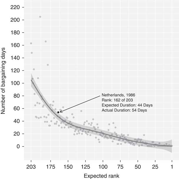
Figure 1 shows an example of this step. The data and model come from Martin and Vanberg’sFootnote 31 research on the duration of coalition government bargaining, which is the first of our replication studies below. The graph gives the expected ranks of the observations on the x-axis – from the smallest values of the linear predictor on the left side of the graph (last to event occurrence) to the largest on the right (first to event occurrence) – against the observed durations on the y-axis.Footnote 32 The solid line represents the GAM fit and the shading indicates its 95 per cent confidence interval. Note the clear downward (but nonlinear) relationship between the durations and the ranks. As an observation’s value of the linear predictor becomes relatively larger (that is, larger relative risk of event occurrence), its actual number of bargaining days decreases, but at a decreasing rate. This nonlinearity is captured by the GAM.
GAM fit of the observed durations against expected ranks from the Martin and Vanberg (2003) Cox model Note: The graph plots the expected ranks of the observations on the x-axis (descending order) against the observed durations on the y-axis. The solid line and shading indicate the GAM fit and its 95% confidence interval.

Next, expected durations can be computed for observations in the data, similar to generating expected values of the dependent variable from a linear regression model. To do this, Cox ED uses the GAM fit to compute the expected value of the duration given the observation’s rank. The solid line in Figure 1 shows these values for the Martin and Vanberg model.Footnote 33 As an example, consider the observation highlighted in black (Netherlands, 1986). That observation’s rank is 162 (x-axis), which corresponds to an expected duration of about forty-four days according to the GAM (y-axis). Note also that the actual duration for that observation is fifty-four days (the black point). Thus, the GAM is off by about ten days. We utilize the differences between these expected values and the actual durations as a means of assessing the performance of the Cox ED methods in our simulations (see the Appendix).
In order to examine marginal changes in duration given a change in a covariate, it is necessary to create two or more ‘new’ observations corresponding to theoretically interesting, hypothetical covariate profiles. For instance, we might set an indicator variable to 0 and 1 or a continuous variable to a ‘low’ and a ‘high’ value.Footnote 34 For the other variables in the model, Cox ED employs the observed value method of Hanmer and Kalkan.Footnote 35 Instead of setting those variables to their means or modes, it allows them to vary naturally over the entire data, then averages over them in the computations.Footnote 36 For instance, to estimate the effect of an increase in a covariate X 1 from 0 to 1 on the expected duration, we use the following steps:
(a) Set X 1 to 1 for the entire data (all N observations) and calculate the ELP for every observation, then take the average value of those computations (the median is the default).Footnote 37
(b) Repeat step (a) while setting X 1 equal to 0.
(c) Take the values obtained in steps (a) and (b) and append them to the list of ELP values from the original Cox model in which X 1 is left as exogenous data. Then compute new rankings of the linear predictor values from this list, which is length N+2.
(d) Pass the list of rankings from step (c) to the GAM as new data to generate expected values. Note that a new GAM is not estimated at this step. Rather, expected durations are generated for each observation – including the two new ones created in steps (a) and (b) – using the previously estimated GAM. This produces point estimates of the expected durations for those two new observations.
(e) Compute the difference between the two estimates obtained in step (d): the expected duration for the data in which X 1 is set to 1 and the expected duration for the data in which X 1 is set to 0. This quantity is a point estimate for the marginal effect, or first difference, corresponding to the change in X 1 from 0 to 1.
Finally, to produce estimates of uncertainty, the GAM approach repeats this process many times (1,000 is the default) via bootstrapping. The method generates bootstrap samples of the data and re-estimates the Cox model coefficients on each bootstrap sample.Footnote 38 At each iteration, this produces a new vector of actual durations and a new ranking of ELP values, which are then used to fit a new GAM. This results in a distribution of expected durations for each independent variable profile (for example, step d) and a distribution of the marginal effect (step e). These distributions can be used to produce standard errors and confidence intervals for the estimates.Footnote 39 Importantly, by bootstrapping the entire process, this step incorporates the uncertainty from the Cox model estimation and the uncertainty from the GAM.Footnote 40
This process is mostly automated in our software; analysts need only an estimated Cox model, the name of the variable of interest and the two values of that variable they wish to input. However, the functions also allow for several changes to default settings, including the formulation of the GAM and the computation of confidence intervals. Additionally, it can be used with models that include time-varying covariates (see our replication of Box-SteffensmeierFootnote 41 in the Appendix).Footnote 42
The Nonparametric Step-Function Approach
Another approach to calculating expected durations and marginal changes in expected duration from the Cox model derives from the method proposed by Cox and OakesFootnote 43 for estimating the cumulative baseline hazard function. This method is nonparametric and results in a step-function representation of the cumulative baseline hazard; therefore we refer to the following technique as the nonparametric step-function (NPSF) approach. We begin by describing the Cox and Oakes method, then we explain how we extend this method to estimate expected durations. While the NPSF method is an established procedure for estimating the cumulative baseline hazard, our extension of the method is novel.
Cox and OakesFootnote 44 show that the cumulative baseline hazard function can be estimated after fitting a Cox model by
 $$\hat{H}_{0} \left( t \right)\,{\equals}\,\mathop{\sum}\limits_{\tau _{j} \,\lt\,t} {{d_{j} } \over {\mathop{\sum}\limits_{l\,\in\,\Re \left( {\tau _{j} } \right)} \hat{\psi }\left( l \right)}},$$
where τ
j
represents time points earlier than t, d
j
is a count of the total number of failures at τ
j
,
 $$\Re (\tau _{j} )$$
is the remaining risk set at τ
j
, and
 $$\hat{\psi }(l)$$
represents the ELP from the Cox model for observations still in the risk set at τ
j
. We use equation 1 to calculate the cumulative baseline hazard at all time points in the range of observed durations.Footnote
45
This estimate is a stepwise function because time points with no failures do not contribute to the cumulative hazard, so the function is flat until the next time point with observed failures.
We extend this method to obtain expected durations and marginal changes in expected duration by first calculating the baseline survivor function from the cumulative hazard function, using
 $$\hat{S}_{0} \left( t \right)\,{\equals}\,exp\left[ {{\minus}\hat{H}_{0} \left( t \right)} \right].$$
Each observation’s survivor function is related to the baseline survivor function by
 $$\hat{S}_{i} \left( t \right)\,{\equals}\,\hat{S}_{0} \left( t \right)^{{\hat{\psi }\left( i \right)}} ,$$
where
 $$\hat{\psi }(i)$$
is the ELP for observation i. These survivor functions can be used directly to calculate expected durations for each observation. The expected value of a non-negative random variable can be calculated by
 $$E\left( X \right)\,{\equals}\,{\int}_0^\infty \left( {1{\minus}F\left( t \right)} \right)dt,$$
where F (.) is the cumulative distribution function for X. In the case of a duration variable t i , the expected duration is
 $$E\left( {t_{i} } \right)\,{\equals}\,{\int}_0^T S_{i} \left( t \right)\:dt,$$
where T is the largest possible duration and S i (t) is the individual’s survivor function. We approximate this integral with a right Riemann-sum by calculating the survivor functions at every discrete time point from the minimum to the maximum observed durations, and multiplying these values by the length of the interval between time points with observed failures:
 $$E\left( {t_{i} } \right)\approx\mathop{\sum}\limits_{t_{j} \in[0,T]} \left( {t_{j} \,{\minus}\,t_{{j{\minus}1}} } \right)S_{i} \left( {t_{j} } \right).$$
Finally, to calculate a marginal effect, we follow the same strategy that we employ in the GAM approach. We create two new covariate profiles, setting a variable of interest to two theoretically interesting values. We use the method described above to calculate expected values from each profile. We then compute the difference in the two estimates, and bootstrap to obtain a standard error and/or confidence intervals for this point estimate.
Choosing between GAM and NPSF
An important consideration for applied researchers who use Cox ED is the choice of method. Both have strengths and weaknesses which should be carefully weighed in the context of the data and model. The GAM approach is intuitive and shows good empirical performance in our replications and simulations (see below and the Appendix). NPSF displays good performance as well, but it is more complex. The main advantage of NPSF over the GAM approach is that the former is more elegant. It is derived directly from the assumptions of the Cox model and does not require an ad hoc estimation of a second model (the GAM). We view this as a legitimate reason for preferring NPSF over the GAM approach.
Nonetheless, we maintain a slight general preference for the GAM approach over NPSF. One reason for this is that the GAM approach is a bit more flexible because it can accommodate TVCs. Additionally, while our simulations show that both methods display similar performance in returning the correct point estimate, the GAM method produces better measures of uncertainty (particularly in small samples). We show simulation results evaluating the coverage of the confidence intervals of each method (see the Appendix). There we demonstrate that the GAM method’s confidence intervals are closer to covering at the nominal level compared to NPSF. In short, we recommend that researchers use the GAM approach as a starting point and consider using the NPSF approach if they have a specific preference for the single-model estimation strategy.
APPLYING COX ED TO POLITICAL SCIENCE
We next demonstrate the application of Cox ED to actual data used in political science. We reanalyze four published papers that employ the Cox model to assess the extent to which Cox ED can help political scientists better understand the substantive implications of their results. These papers span three subfields – comparative politics,Footnote 46 American politicsFootnote 47 and international relations.Footnote 48 We replicated the Cox model in each article, then employed one of our Cox ED procedures to assess the substantive effects of key independent variables. Our goal with these replications is not to critique the authors’ modeling choices, but rather to demonstrate how Cox ED can help applied researchers present Cox model results with more meaningful quantities. In doing so, we uncover novel substantive insights in each example. We present the replications of Martin and VanbergFootnote 49 using the GAM approach and Box-Steffensmeier, Arnold and ZornFootnote 50 using the NPSF approach here. To conserve space, we present replications of Box-SteffensmeierFootnote 51 using GAM with time-varying covariates, and Mattes and SavunFootnote 52 using the GAM approach in the Appendix.
Coalition Bargaining and Government Formation
Martin and VanbergFootnote 53 examine the determinants of negotiation time among political parties forming a coalition government. In particular, they are interested in the effects of ideological distance between the parties in the coalition as well as the size of the coalition. They use data on government formation in ten European countries from 1950 to 1990 to test two hypotheses, both of which they posit using the language of time. Specifically, they expect that negotiations ‘conclude more quickly’ (1) when bargaining parties are ideologically close and (2) when there are fewer parties engaged in bargaining.Footnote 54
The dependent variable in Martin and Vanberg’s analysis is the number of days between the beginning and end of the bargaining period. Martin and Vanberg model this variable as a function of the Range of government, which is a measure of the ideological distance between the extreme members of the coalition, the Number of government parties in the coalition, and several other variables. They interact Number of government parties with the natural log of time because that variable violates the proportional hazards assumption. Their hypotheses predict negative coefficients on the variables of interest, indicating that increases in the ideological distance between the parties and in the number of parties correspond with a decrease in the risk of government formation, or a longer negotiation time.
The authors demonstrate support for their hypotheses by computing changes in the hazard rate based on changes to these independent variables. Regarding the estimated effect of Range of government, they state the following: ‘an increase in the ideological range of the government from zero (the case of a single-party government) to 1.24 (the average range for coalition governments in our sample) decreases the odds of government formation on any given day in the bargaining process by approximately 23 per cent’.Footnote 55 On the second hypothesis, they find that ‘for all governments that formed after two weeks of bargaining, negotiations leading to three-party coalitions were on average over 50 per cent less likely to end on any particular day than negotiations leading to two-party coalitions’.Footnote 56 Overall, they conclude that both variables are important determinants of the time it takes governments to form.
Martin and Vanberg’s discussion of the substantive effects of their key variables meets the discipline’s current standards. However, it also highlights our critiques of relying on the hazard rate. For instance, it is difficult to assess what the estimated effects of Range of government and Number of government parties mean in substantive terms. How much longer will negotiations take for a typical coalition government than for a single-party government? How long does each additional party delay the process? Our Cox ED method is able to answer these kinds of questions.
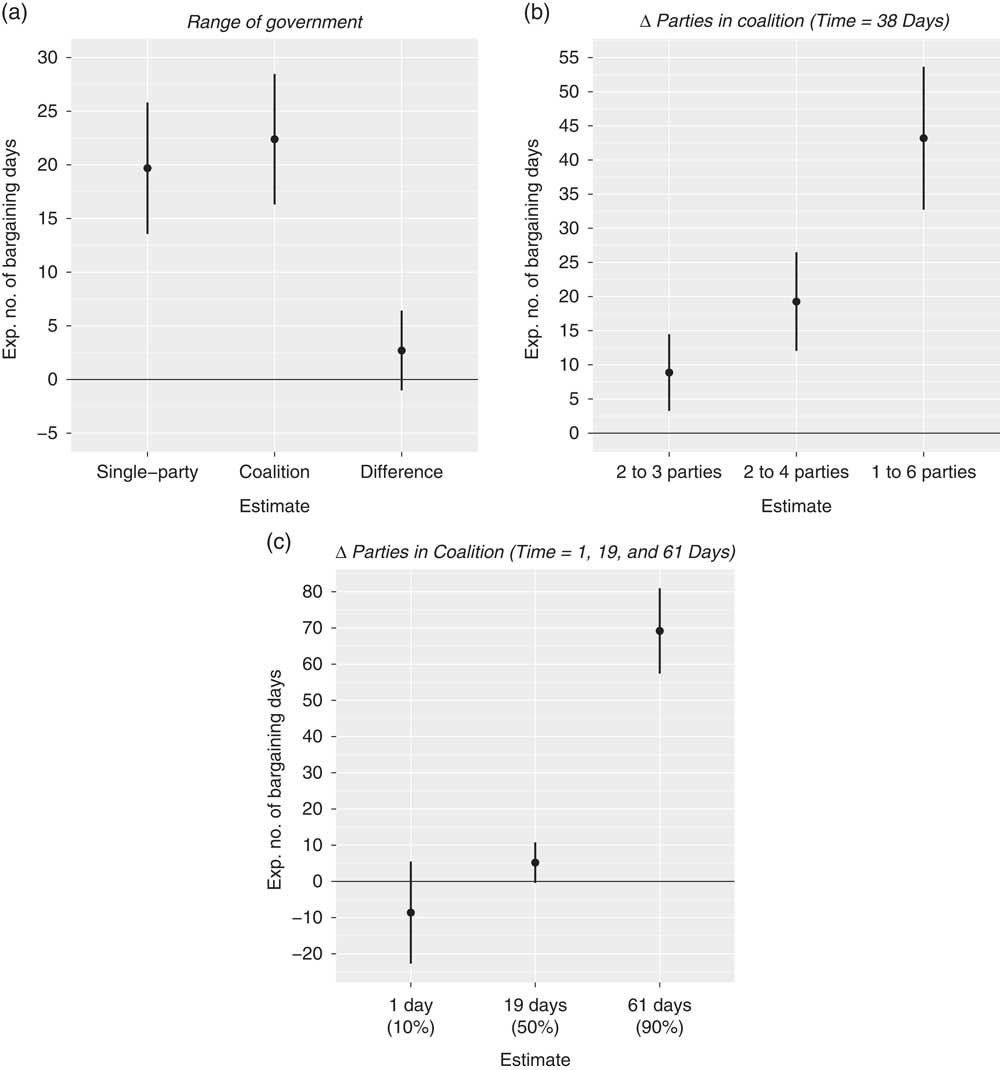
After replicating the model, we utilized the GAM approach to generate expected durations and confidence intervals for different independent variable profiles. Recall from above that these expected durations are generated from a GAM fit of the observed durations on the expected ranks for each observation produced by the Cox model (Figure 1 displays the GAM fit for this example). The authors expect that as the parties in the coalition become ideologically farther apart and/or more parties join the coalition, the risk of government formation decreases. Put differently, this means that as Range of government and/or Number of government parties increases, so too should the expected number of bargaining days. Figure 2 graphs these relationships.
The effects of range of government and number of government parties on the expected number of bargaining days until coalition government formation (Martin and Vanberg Reference Lupia and Aldrich2003) Note: Panel (a) graphs the expected number of bargaining days for a single-party government (Range of government=0) versus the average value for coalition governments (Range of government=1.24) and the difference between the two. Panel (b) graphs the increase in the expected number of bargaining days that corresponds to three different changes in the Number of government parties in the coalition and time set to 38 days (75th percentile). Panel (c) graphs the change in the expected number of bargaining days moving from one to six parties with time set to 1, 19, and 61 days (the 10th percentile, median, and 90th percentiles, respectively). Lines indicate 95% confidence intervals.
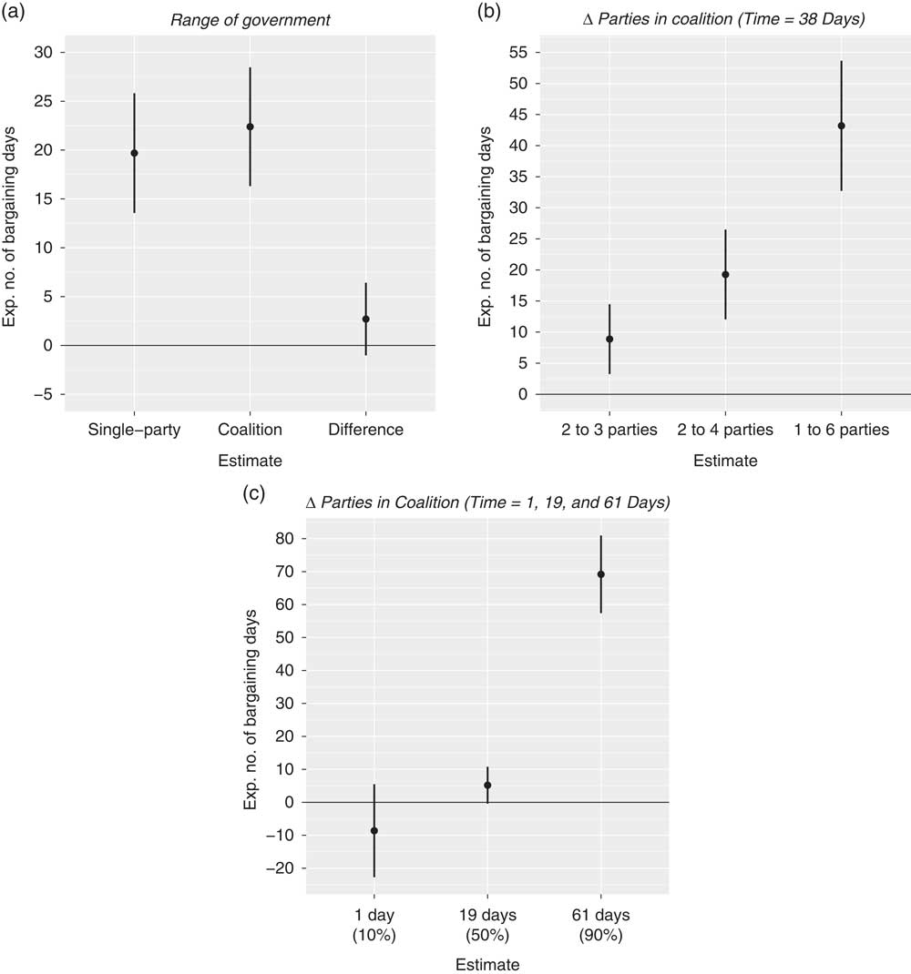
Panel (a) of Figure 2 graphs the expected number of bargaining days for a comparison that Martin and Vanberg consider in their analysis: a single-party government (Range of government=0) versus the average value for coalition governments (Range of government=1.24). Recall that they report that this change results in an expected 23 per cent decrease in the hazard rate. Using Cox ED and averaging over the other variables in the model, we estimate about twenty days until government formation for a single-party government compared to twenty-two days for the typical coalition government. This difference of about two days is relatively small and not statistically significant.
Figure 2, panel (b), shows the effect of Number of government parties with time set to thirty-eight days (its 75th percentile). There we graph the expected increase in bargaining days as a function of three different changes to the number of parties. We estimate that a change from two to three parties corresponds to an increase of nine days, moving from two to four parties lengthens bargaining by nineteen days, and moving along the full observed range from one to six parties makes bargaining longer by almost 1.5 months (forty-three days). All of these differences are statistically significant at the 95 per cent confidence level.
Recall that Martin and Vanberg interact Number of government parties with the natural log of time to address the violation of the proportional hazards assumption. We can use Cox ED to examine the impact of time on the effect of coalition size. Panel (c) presents the change in the expected number of bargaining days moving from one to six parties with time set to one, nineteen and sixty-one days (the 10th percentile, median and 90th percentiles, respectively). The graph shows clear evidence of duration dependence. Adding more parties exerts a substantively small and statistically nonsignificant negative effect on bargaining time early on, but becomes strongly positive and statistically significant later in the process.
In sum, we find that the effect of Range of government is relatively small compared to the effect of Number of government parties, at least when a sufficient amount of time has elapsed. The estimated difference of two days due to a change in Range of government is not statistically significant, and even the smallest change in Number of government parties in panel (b) produces an estimated effect that is over four times as large. This example illustrates the utility of Cox ED in assessing Cox model results. While Martin and Vanberg’s analysis of changes in the hazard rate does show that the effect of Number of government parties is larger than that of Range of government, our analysis adds much more detail about the substantive magnitude of this difference. Moreover, by deriving results in terms of bargaining days, we frame the results in ways that are intuitive, easily understood by a wide audience of readers, and match the authors’ theoretical interests.
The Strategic Timing of the NAFTA Vote
In a well-known article employing the Cox model, Box-Steffensmeier, Arnold and ZornFootnote 57 model the duration until members of the US House took a position on the North American Free Trade Agreement (NAFTA) in 1992–3. They develop hypotheses for several factors, including those related to constituents, organized interests and policy leaders. Importantly, they frame these hypotheses in the language of time. For example, they expect representatives of districts bordering Mexico to ‘announce earlier’.Footnote 58 They expect the time to announcement to drop as a House member’s amount of campaign donations from corporate or labor donors increases. They also posit that Republican leaders announce a position earlier than rank-and-file members, but have no expectations regarding Democratic leaders.
The dependent variable is the number of days after 11 August 1992 that a House member took either a ‘yes’ or ‘no’ position on NAFTA. The authors’ model includes several variables related to their hypotheses, some of which include interaction terms. In some cases they expect positive coefficients and in others they expect negative coefficients.Footnote 59 They show support for some of their hypotheses, communicating the substantive results with percentage changes in the hazard rate and graphs of the survivor function.Footnote 60 This latter approach further indicates that the authors’ main conceptual interest is in the time until position announcement, not the hazard of announcement.
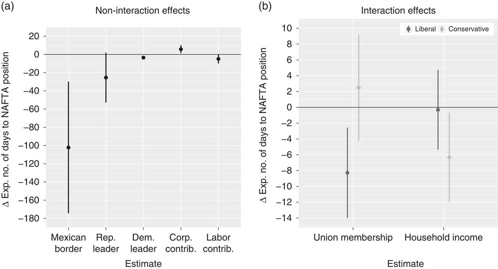
Accordingly, we utilized the NPSF approach to generate estimates of the change in time to announcement corresponding with changes to several independent variables. We report these results in Figure 3. Panel (a) gives the results for the variables that do not include interactive hypotheses. Panel (b) graphs results for two variables which the authors expect to exert a conditional relationship. Specifically, they expect that the effect of Union membership in the district on the time to announcement is negative for liberal House members and positive for conservatives. They also expect that as Household income increases, liberal members take longer to announce and conservatives take less time.
The determinants of timing on the NAFTA vote (Reference Box-Steffensmeier, Arnold and ZornBox-Steffensmeier, Arnold and Zorn 1997) Note: Panel (a) graphs the effects of a change in the non-interactive variables on the expected change in time to announcement (a move from no to yes for Mexican border, Republican leader and Democratic leader and a standard deviation increase for Corporate contributions and Labor contributions). Panel (b) graphs the effects of a standard deviation increase in Union membership and Household income for liberal and conservative members of Congress. Lines indicate 95% confidence intervals.

Box-Steffensmeier, Arnold and Zorn interpret the effect of representing a border district as an increase of 528 per cent in the hazard of announcement.Footnote 61 As we discuss above, it is difficult to put such an estimate into context because percentage changes in the hazard rate have no meaningful scale. Panel (a) of Figure 3 shows more clearly that bordering Mexico corresponds with a substantively large effect on time until a Congressperson announces a position. Using the NPSF approach, we estimate that those in border districts announce a position 102 days sooner, on average. The confidence interval is somewhat large due to the fact the data only contain eleven border district representatives. Nonetheless, this estimate is considerably more conceptually precise and also more intuitive compared to a hazard-based quantity.
The rest of the graph in panel (a) shows that the effects of the other variables are relatively small in magnitude, and are not completely supportive of expectations. For example, as the authors expect additional campaign contributions from labor correspond with a decrease in time to announcement of about five days, but the effect of corporate contributions is an increase of six days, contrary to expectations. In line with expectations, Republican leaders announce a position about twenty-five days sooner compared to rank-and-file members.
Finally, the interaction effects in panel (b) of Figure 3 show mixed support for the authors’ hypotheses. As expected, the effect of Union membership is negative for liberal House members (a drop of about eight days) and positive for conservatives (increase of three days). However, these estimates are fairly small in magnitude; only the estimate for liberals is statistically distinguishable from zero, and the two estimates are not distinguishable from each other at the 95 per cent confidence level. As Household income increases, the change in expected time to announcement is essentially zero for liberal members, but is a statistically significant drop of about six days, as expected, for conservatives.
As in our first example, this replication shows the utility of the Cox ED method. All Congresspersons eventually took a position on NAFTA because the House voted on the bill in November 1993. Thus, the hazard of position-taking is not the concept of chief theoretical interest. Indeed, in discussing their theoretical framework Box-Steffensmeier, Arnold and Zorn emphasize that there is a strategic political calculation in the timing of members’ position-taking. Accordingly, we contend that quantities computed from their model should reflect those strategic calculations and say something about expected time to announcement. Cox ED permits this sort of interpretation.
CONCLUSIONS
The Cox model is, for good reason, a popular choice among researchers in political science as well as several other disciplines. The ability to estimate a survival model while leaving the baseline hazard function unspecified makes the Cox model a major contribution to applied statistics. However, this flexibility limits the quantities that analysts can compute from their results. The typical means of interpreting model results involves multiplicative changes in the hazard rate of event occurrence. This approach leads to substantively vague estimates of covariate effects that are challenging to effectively communicate, especially to non-academic consumers of research. Moreover, it does not match the chief conceptual interest of many researchers who employ the Cox model: the duration of some phenomenon.
As a solution, we present Cox ED, a suite of methods for computing expected durations for the observed data or new observations with substantively interesting covariate profiles (which can include time-varying covariates), as well as marginal changes in these expected durations as a result of a change in a covariate. Our replications of published studies that employ the Cox model show that these expected durations are useful for substantive discussions of model results. Expected durations are easy to interpret, closely reflect the substantive goal of survival analysis and can be easily understood by academics, students, journalists and public officials.
Practically speaking, Cox ED is straightforward to implement in R and Stata. Our software packages contain functions that allow researchers to easily use the methods after estimating a Cox model. Additionally, the functions are flexible; users can make several changes to many of the features of the methods that we describe above. The output from the functions provide point estimates, standard errors and confidence intervals, so researchers can report their results with appropriate measures of uncertainty.
Of course, researchers have always had the ability to generate expected durations from a parametric duration model; we do not claim to have developed the quantity for the first time here. However, the parametric models for which expected durations are available force researchers to make an assumption about the baseline hazard function. This assumption may not be correct and is never truly testable. So it is no surprise that the Cox model is a well-used tool in applied work. The main drawback to its popularity is that the substantive clarity of interpretation of results lags behind that of other common statistical models, such as linear regression or logistic regression. Cox ED solves this problem. The method provides the benefit of the intuitive quantities available in parametric models while retaining the desirable estimation properties of the Cox model.