

1 Introduction
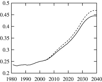
The purpose of this paper is to illuminate the macroeconomic relevance of education and human capital formation in an aging society. This topic has received much attention over recent years, mainly due to the expected sharp increase in the share of the retired over the working population (cf. Figure 1). Moreover, older workers are leaving the labor force at younger and younger ages.Footnote 1 This decline in labor force participation, which magnifies population trends, is due to specific characteristics of existing pension systems, which impose considerable negative accrual rates of pension wealth.
Dependency ratio projections for Switzerland. The solid line shows the trend extrapolation, the dashed line a more pessimistic scenario

In order to compensate for the adverse effects of the shift in the age structure on production, labor productivity of the working needs to increase or retirement must be postponed.Footnote 2 We analyze the direct effect of a change in the age structure due to aging on the individuals' incentives to invest in education at the extensive margin. Indeed, aging itself strongly affects the skill structure of the workforce by changing the distribution of the workers' seniority. However, additional policy measures towards increased human capital investment would have to be put in place in order to maintain total employment and to assure the financial viability of existing pension systems. We show that postponed retirement raises educational attainment and human capital. However, it induces individuals to save less, which offsets these beneficial effects.
In this paper, individuals' intensive and extensive education decisions are studied, along with their intertemporal consumption choice and labor supply. To be able to simulate a concrete population and policy scenario, the model realistically reproduces (1) individual life cycle wage and consumption profiles; (2) the skill composition in the labor force; (3) skill premia in wages; (4) the change in relative prices and the production structure due to an aging population and postponed retirement. We use an overlapping generations (OLG) approach in general equilibrium in order to be able to analyze intergenerational distribution effects.
The remainder of this paper is organized as follows. We first give a short overview of the literature related to our subject. Based on the probabilistic aging approach, we then motivate our modeling of the production technology allowing for capital–skill complementarity. Third, we present a stylized model in order to highlight the important economic effects showing up in our quantitative analysis. We then discuss the calibration of the model. Finally, we simulate the effects of aging and postponed retirement on key macro variables in an open economy setting.
2 Related literature
In its complexity, the model relates to four strands of economic literature:
Education and the economy Besides the vast literature on life cycle human capital investment, which focuses on the intensive margin of education, there is a strand of literature concentrating on the extensive margin.Footnote 3 This mostly empirical literature is concerned with self-selection of students into skill types according to ability types which affects estimates of occupational choice and the distribution of earnings. The first source is Roy (Reference Roy1951), which has received subsequent elaboration, e.g. by Heckman and Honoré (Reference Heckman and Honoré1990). Willis and Rosen (Reference Willis and Rosen1979) and Heckman et al. (Reference Heckman, Lochner and Taber1998) derive a theoretical model of the demand for college attendance and empirically show that expected life-time earnings indeed influence the college attendance choice decisively. Due to the specific nature of their sample, there is no ability bias in the estimation of the enrollment function, a problem which is often encountered in the empirical assessment of the rate of return to education. Bils and Klenow (Reference Bils and Klenow2000) argue that not only schooling leads to higher growth rates, such as in Barro (Reference Barro1991), but that there is also a reverse channel through which faster growth can induce more schooling by raising its effective return.
Overlapping generations Economic models with overlapping generations of households provide a good basis for the analysis of fiscal policy and intertemporal macroeconomics. There are basically two strands of OLG literature: The one with a large number of generations and detailed life-cycle patterns pioneered by Auerbach and Kotlikoff (Reference Auerbach and Kotlikoff1987) with refinements by for example, İmrohoroğlu et al. (Reference İmrohoroǧlu, İmrohoroǧlu and Joines1999) and Altig et al. (Reference Altig, Auerbach, Kotlikoff, Smetters and Walliser2001). The second strand is based, upon the model by Ramsey (Reference Ramsey1928) with infinitely lived consumers. Blanchard (Reference Blanchard1985) introduces constant mortality hazard, which leads to potentially finite life times but eternal youth. The model by Gertler (Reference Gertler1999) introduces life-cycle behavior in this framework by allowing mortality only for the retired. We base our approach on its consequent enhancement by Grafenhofer et al. (Reference Grafenhofer, Jaag, Keuschnigg and Keuschnigg2005), who introduce probabilistic aging, which allows for mortality among young ages and thereby exhibits a closer approximation of the demographic structure.
Old-age provision There is a vast literature on the economics of old-age provision, arguing that its design considerably affects labor market participation and early retirement.Footnote 4 Sanchez-Martin (2003) and Keuschnigg and Keuschnigg (Reference Keuschnigg and Keuschnigg2004) use computable general equilibrium (CGE) models to analyze how pension system reforms may be able to alleviate the expected financial difficulties of current PAYG systems. Lau and Poutvaara (Reference Lau and Poutvaara2000, Reference Lau and Poutvaara2001) study the impact of social security incentives on human capital formation, arguing that actuarial fairness and a tight contributions–benefit link increase human capital along with an increase in the retirement age. İmrohoroğlu et al. (Reference İmrohoroǧlu, İmrohoroǧlu and Joines1995) derive optimal social security replacement rates and associated benefits by means of an applied general equilibrium model.
Demographic transition The demographic transition in industrialized countries with lower fertility and higher life expectancy poses challenges to pension systems and the economy as a whole (cf. e.g. Miles, Reference Miles1999; Börsch-Supan and Winter, Reference Börsch-Supan and Winter2001; Bovenberg and Knaap, Reference Bovenberg and Knaap2005). Börsch-Supan (Reference Börsch-Supan2003) argues that in order to finance the pension system, contribution and tax rates will have to rise, which reduces labor force participation of the younger cohorts and destabilizes the pension system even more. In a model with imperfect substitutability between less and more experienced workers, Rojas (Reference Rojas2005) shows that the effects of aging are less hazardous than with perfectly substitutable workers. Also, Conesa and Krueger (Reference Conesa and Krueger1999) consider heterogeneous agents and their impact on the political support for a funded pension system.
Besides its adverse effects on the pension system, population aging may induce individuals to invest more in education.Footnote 5 The contribution of this paper is an analysis of this effect by means of a model featuring a realistic production structure with differentiated labor inputs and coherent education decisions in a general equilibrium model with overlapping generations based on probabilistic aging, as developed in Grafenhofer et al. (Reference Grafenhofer, Jaag, Keuschnigg and Keuschnigg2005) and Jaag et al. (Reference Jaag, Keuschnigg and Keuschnigg2005).
3 Capital–skill complementarity
Many life-cycle models with overlapping generations, such as the original Auerbach and Kotlikoff (Reference Auerbach and Kotlikoff1987) model, but also, for example, Altig et al. (Reference Altig, Auerbach, Kotlikoff, Smetters and Walliser2001) assume labor to be homogeneous. Recently, heterogeneous labor has been introduced in various ways: Heckman et al. (Reference Heckman, Lochner and Taber1998) use labor which is differentiated by skill level, while Rojas (Reference Rojas2005) uses a labor market characterized by imperfect substitutability between less and more experienced workers, hence introducing a vertical differentiation of labor. In our model, the individuals' discrete education choice leads to a partition of the working population into different skill classes, which is mirrored on the production side, where the firms' technology uses as inputs differentiated labor and capital, hence giving rise to a horizontal differentiation of labor. For simplicity, we assume that the experience of workers does not alter their type of labor.
The surge in skill-biased information technology during the 1990s, which coincided with a rise in the wages of skilled workers relative to those of unskilled workers, suggests that various kinds of labor are of different substitutability with capital. The first evidence of this phenomenon is due to Griliches (Reference Griliches1969), who refers to his finding that capital and skilled labor are more complementary as inputs than are capital and unskilled labor as the capital–skill complementarity hypothesis. The hypothesis has received broad attention in the macroeconomic literature, where evidence in its favor has important implications on how to specify aggregate production in theory, but also in reassessing the robustness of existing empirical findings. Quantitative implications of the hypothesis are studied, for example by Duffy et al. (Reference Duffy, Papageorgiou and Perez-Sebastian2004) who find only weak evidence in support of it, however. The hypothesis has also been tested in many microeconomic studies with firm and industry-level data. For a representative sample of such studies see Hamermesh (Reference Hamermesh1993), who concludes that there is strong evidence for capital–skill complementarity. However, he cautions that many of the studies that disaggregate the workforce by demographic group exclude capital as a productive input due to the lack of a reliable measure of the capital stock. The assumption of competitive markets allows early studies to proxy variations in the capital stock by variations in the rates of return. More recent studies refrain from this assumption and explicitly include the stock of capital in their analysis (cf. Duffy et al., Reference Duffy, Papageorgiou and Perez-Sebastian2004).
Goldin and Katz (Reference Goldin and Katz1998) argue that physical capital and skills have not always been viewed as relative complements: In an earlier era, the transformation from skilled artisan shops to factories involved the substitution of physical capital and unskilled labor for highly skilled labor – precisely the opposite of what is hypothesized to be happening today. This suggests that capital–skill complementarity may be a transitory phenomenon: in a country's development process, skilled labor may change from being well substitutable with capital and unskilled labor to being highly complementary to these two inputs. In order to account for this, recent studies consider panel data over long periods of time (e.g. Duffy et al., Reference Duffy, Papageorgiou and Perez-Sebastian2004) or split the full country sample into subsamples of similar development (e.g. Papageorgiou and Chmelarova, Reference Papageorgiou and Chmelarova2005). A consistent finding also supported by Galor and Weil (Reference Galor and Weil2000) is that the capital–skill complementarity is especially strong at the beginning of a development process and may fade out when a technology becomes widely adopted.
The observed increase in the skill premium during the 1990s in developed countries may be due to skill-biased technological change, as is brought forward, for example, by Acemoglu (Reference Acemoglu1998) who argues that an increase in the supply of skills reduces the skill premium in the short run, but induces biased technological change and hence increases the skill premium in the long run. Krusell et al. (Reference Krusell, Ohanian, Rios-Rull and Violante2000) challenge this view in an empirical study, where they find that with capital–skill complementarity, changes in observed inputs in the aggregate production function alone account for most of the variations in the skill premium.
To our knowledge, the approach in this paper is the first to employ a production technology with potentially many types of labor and capital–skill complementarity in a general equilibrium OLG framework. We start by describing a stylized model exemplifying the main channels, through which the shocks in the scenarios affect economic outcomes in our model. The building blocks of the actual CGE model are described in the appendix.
4 Illustrative simple model
As discussed in Jaag et al. (Reference Jaag, Keuschnigg and Keuschnigg2005), the human capital accumulation process over the life cycle can be analyzed independently of other life cycle choices, such as optimum consumption and leisure. Therefore, in this section, we concentrate on extensive and intensive education decisions and on the specifics of the production technology.
4.1 Production technology
For an illustration of capital–skill complementarity in production, consider the simple production function

where capital K and unskilled labor L 1 are perfect substitutes and have unit elasticity of substitution with skilled labor L 2.Footnote 6 The ratio of the marginal products of skilled to unskilled labor, and accordingly the relative wage of high-skilled labor, is
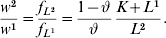
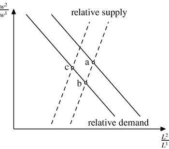
This will determine human wealth in the respective skill classes and govern the extensive education decision at the beginning of the life cycle. It also constitutes the relative labor demand in Figure 4.
4.2 Human capital production
For the illustrative purpose of this section, we consider two different types of human capital s∊{1, 2}, which constitute skilled and unskilled labor, respectively. Low-skilled productivity is denoted by θ1, while high-skilled productivity is θ2. Time and individual ability are the only inputs of human capital production (cf. Figure 2): Over her life cycle, an individual spends her time on education up to date e. Then, she works with exogenously given intensity until retirement at date R.
An individual's activity over the life cycle

We assume that individual ability ι is relatively more important in acquiring high-skilled human capital. These characteristics of human capital accumulation are formalized as


Note that for simplicity, θ1 is independent of ι.Footnote 7 Individuals maximize their human capital, i.e. their life-time earnings. The problem of an individual with ability ι is therefore to choose the type of human capital s ι and the optimal education time spent on its accumulation e sι given the retirement date R ι and the wage rate w s per unit of human wealth, such that

The benefit of a longer education period is an increase in productivity during the working period. The cost consists of a shorter work life. For any individual of ability ι there is a unique time investment, which maximizes life-time earnings from any type of human capital


Since ability enters both benefit and cost symmetrically, there are no differences in education among individuals of different ability. The resulting skill levels are therefore, by (2) and (3)

Hence, optimum skill acquisition is proportional to the expected length of the working period, and only θι2 depends on the ability of the individuals in that skill group.
4.3 Extensive education decision
The type of human capital an individual chooses to acquire – measured as the sum over all life-time earnings – results from a comparison of the respective levels of human wealth
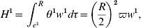
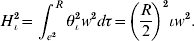
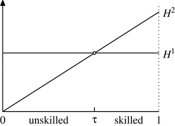
Individuals with higher ability have a comparative advantage in the acquiring of skills, and the human capital of those investing in skills increases monotonically in the ability parameter, cf. Figure 3.
Discrete choice between two skill groups

An individual is indifferent between acquiring low-skilled and high-skilled human capital iff

Hence, using (6) and (7), the pivotal (indifferent) worker type

is determined by

The relative size of the two skill classes is determined by the relative wage, which itself by (1) depends on the skill structure in the economy. The total number of efficiency units in each skill class is given by the employment duration, R−e s, times the number of workers times their human capital. Assuming skills to be distributed uniformly over the unit interval, ι~U (0, 1), and normalizing the total number of workers to unity, the number of low-skilled workers is equal to N 1=
. The number of high-skilled workers is accordingly N 2=1−
. The size of the two labor forces in efficiency units is then given by
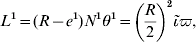

Relating (9) to (6), we see that the total wage bill for unskilled labor, w 1L 1 just equals total human capital H 1N 1. Substituting (8) for
, we get
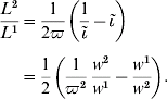
This yields the increasing relative labor supply curve in Figure 4 below.
Dynamic effects of capital–skill complementarity

4.4 Equilibrium
The equilibrium is characterized by a stratification of individuals according to (11), which determines the relative size of the two skill classes, wages and intensive education levels. Inserting (1) and (9)/(10) into (8), we implicitly get the equilibrium pivotal worker type
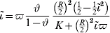
as a function of the relative importance of the two labor types in production ϑ, the level of the capital stock K, the retirement date R, and the relative productivity of time in educational production ϖ.
Since the demand for labor is – by the capital–skill complementarity – tightly linked to the capital stock, we first analyze the equilibrium reaction of education to changes in capital. The responses of intensive and extensive education to an increase in the capital stock are
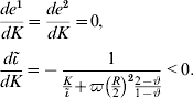
Educational effort at the intensive margin is not influenced by a change in the capital stock since the costs of education consist only of foregone earnings, and a change in marginal productivity affects both costs and benefits equally. Figure 4 displays the effect of a decrease in the capital stock at the extensive margin. As long as the relative supply of low- and high-skilled labor is unchanged, by the complementarity of capital and skilled labor, the relative demand for skilled labor shifts to the left, moving the equilibrium from point (a) to (b). The resulting decrease in the skill premium induces less workers to acquire skills, which shifts the relative supply for skilled labor to the left, leading to the final equilibrium at point (c).
An increase in the retirement age affects education both at the intensive and the extensive margins. We find that in equilibrium the comparative static effects of postponed retirement on extensive and intensive education are
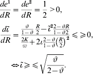
Educational effort is increased by a prolongation of the redemption period. At the extensive margin, education increases as long as the relative size of the high-skilled workforce is below a certain threshold, which is determined by the relative importance of capital and low-skilled labor and high-skilled labor in the production process: with a high importance of skilled labor, postponed retirement will likely increase its share.
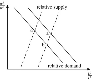
Relative supply remains unchanged initially, as both labor forces grow in parallel. According to (1), relative demand shifts to the left, moving the equilibrium from (a) to (b) in Figure 5. Again, the resulting decrease in the skill premium induces less workers to acquire skills, which shifts the relative supply for skilled labor to the left. Considering (9) and (10), the size of this shift depends on the initial relative sizes of the two workforces. The shift in relative supply leads to the final equilibrium at point (c). Depending on the parameter constellation, the relative wage has risen or fallen in the new stationary equilibrium.
Dynamic effects of postponed retirement

5 Calibration
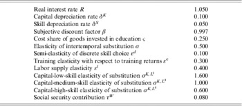
Our simulations are based on the discrete-time model developed by Jaag et al. (Reference Jaag, Keuschnigg and Keuschnigg2005), incorporating probabilistic aging and frictional labor markets.Footnote 8 Important features of this model are detailed in the appendix. We calibrate the model to stylized data of Switzerland in 2000. Table 1 states key parameters characterizing preferences and technology. The choice of the most important parameters is detailed in the following sections by referring to the relevant literature.


Studies on the depreciation rate of human capital range between 1% and 12% (cf. Heckman, Reference Heckman1976; Haley, Reference Haley1976; Lechner and Vazquez-Alvarez, Reference Lechner and Vazquez-Alvarez2005; and the review by Browning, Hansen, and Heckman, Reference Browning, Hansen, Heckman, Taylor and Woodford1999). In the applied literature, very low values are used: zero by Heckman et al. (Reference Heckman, Lochner and Taber1998) and 0.025 by Perroni (Reference Perroni1995). We employ a value of 0.05. Following the literature, we calibrate the depreciation rate of physical capital to 0.1.
5.1 Mortality and transition probabilities
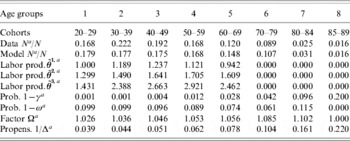
Individual aging occurs not deterministically (cf. Section 8.1 in the appendix): In every period, there is a probability of aging w a. There is also an age-group specific mortality probability 1−γa. Let N a denote the number of individuals in age group a. A tilde indicates the decomposition in annual cohorts, such that N a≡Ñ t. For simplicity, we consider a demographic stationary state and ignore time indices in this section. We further assume that aging parameters are equal across skill groups. Setting w a=0 implies that an aging event occurs with probability one in each period, leading to

. The concept of an age group thus becomes identical with a cohort, where age t is measured by time since birth. Taking age-dependent survival rates

from official mortality tables, the cohort composition of the population in a demographic steady state can be constructed. Recursively applying

yields the size of cohort t relative to the size of a new cohort. Summing up over all cohorts fixes the size of the new cohort compared to total population size N
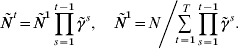
Taking a total length of life of T years, and based on actual survival rates, we have thus found the stationary decomposition of the population into a total of T cohorts. Using the population decomposition indicated in Table 2, each age group contains several cohorts

Given that the instantaneous probability of staying in the current age group is ωaγa, the expected duration in group a is

where αa denotes the time when age group a is entered. The chosen age group decomposition of the actual population corresponds to a life cycle history where an agent spends exactly the average duration in each age period. One can thus recover the demographic parameters of the model from our knowledge of aggregated population data N a and duration in group a. In a demographic steady state, each age group must fulfill the restriction

At this stage, one knows N a from aggregated population data and γaw a from the age group duration as implied by the chosen aggregation. The only unknown in (12) is γa−1, which is easily solved for all groups except the last one. For the last group, γA follows directly from (12) on account of the restriction w A=1. For all age groups a<A, γa can now be recovered recursively.


Individuals enter our model at age 20. We exclude ages 0–20 from the analysis for two reasons: first, in our model setting, the extensive schooling decision as described in Section 8.3 in the appendix is considered to make up the initial condition for on-the-job training, and, second, the actual survival function cannot be easily approximated as the mortality hazard is non-monotonous.
Table 2 shows our decomposition of the population from ages 20 to 90. The aging pattern corresponds to a life cycle biography α=(20, 30, 40, 50, 60, 70, 80, 85), which serves as an aggregation key. It allows for a statement about the size and law of motion of the various age groups. The parameters γa and w a and the inflow into age group 1, N 1t+1,t+1, are chosen such that the stationary solution to (15)–(18) in the appendix corresponds to line 3 in Table 2.
5.2 Intertemporal substitution
In the literature, much effort has been devoted to accurately pin down the value of the rate of intertemporal substitution. On the one hand, macroeconomists use a large value in general, reflecting a common view that a high degree of intertemporal substitution is more consistent with aggregate data considering dynamic macroeconomic models. In their seminal paper, Kydland and Prescott (Reference Kydland and Prescott1982) calibrate it to 0.66, and Lucas (Reference Lucas1990) argues that an elasticity of 0.5 appears too low when confronted with macro data. Laitner and Silverman (Reference Laitner and Silverman2005) estimate it to be as high as 0.87. Also, Weil (Reference Weil1989) finds that in order match growth and business cycle facts, the intertemporal rate of substitution is required to be close to unity. In an influential paper, Hall (Reference Hall1988) shows that consumption growth is completely insensitive to changes in interest rates and, therefore, intertemporal elasticity is close to zero. Guvenen (Reference Guvenen2003) argues that this apparent contradiction arises from ignoring heterogeneity across individuals with respect to stock market participation and wealth. The properties of aggregate variables directly linked to wealth, such as investment and output are entirely determined by high-elasticity stockholders, while aggregate consumption, which is more evenly distributed across households, uncovers the low elasticity of most households. In accordance with the literature on life cycle modeling, we calibrate the elasticity of intertemporal substitution to 0.5 and check for robustness with values of 0.3 and 0.7.
5.3 Skill structure and labor market
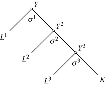
In order to account for the established difference between labor of various skill levels in their substitutability with capital, we use a nested CES production function commonly used in the relevant empirical literature; specific to our setting is the inclusion of more than two skill classes. Every differentiated input factor in the production function makes up for an input level in the nesting structure, as shown in Figure 11 below. We concentrate on the analysis of three differentiated skill classes, which is a realistic reproduction of the education structure in Switzerland.
With the skill choice given by (26) in the appendix, the cost parameter ξs of extensive education is calibrated using
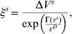
where Γ(v s) can be recovered from the skill distribution of the 20 year olds in the population. As to the extensive skill choice, Heckman et al. (Reference Heckman, Lochner and Taber1998) find that an increase in college tuition of $1,000 (or – equivalently – a decrease in the present value of after-tax earnings) decreases the probability of attending college by about 0.08. This estimate is slightly higher than the estimate by Kane (Reference Kane1994) who finds an according decrease by 0.05 (cf. also Dupor et al., Reference Dupor, Lochner, Taber and Wittekind1996). There is no clear direct empirical evidence on the effect of wage differentials on the extensive education decision. Topel (Reference Topel, Ashenfelter and Card1999), Card and Lemieux (Reference Card and Lemieux2000), and Cunha et al. (Reference Cunha, Heckman and Navarro2005) suggest that teenagers use information on the wage gaps between different attainment levels to evaluate the size of their own future returns to schooling. Since there are many more factors influencing high school and university attendance, such as credit constraints and uncertainty about future earnings, we use a value of 0.1 for the semi-elasticity of the extensive skill choice with respect to differences in indirect utility.
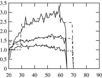
The three skill classes refer to individuals whose highest level of education is secondary I, secondary II, and tertiary, respectively. Table 3 shows the according ISCEDFootnote 9 levels of our skill classes along with their relative population and labor income shares. The skill class and age group specific productivity parameter θ is calibrated using wage data from Switzerland, 2000. The shapes of individual wage profiles are displayed in Figure 6.


The income share of capital is chosen to be 0.35 (cf. İmrohoroğlu et al., Reference İmrohoroǧlu, İmrohoroǧlu and Joines1995 and Conesa and Krueger, Reference Conesa and Krueger1999, who choose 0.36). The empirical evidence on the static labor supply elasticity is reviewed by Hansson and Stuart (Reference Hansson and Stuart1985) and Blundell and MaCurdy (Reference Blundell, MaCurdy, Ashenfelter and Card1999). The latest, most advanced studies yield estimates of the uncompensated wage elasticity of labor supply between 0.05 and 0.12 for men and 0.3 and 1 for women. We calibrate the labor supply elasticity to 0.4.
Following Lord (Reference Lord1989) and Trostel (Reference Trostel1993) we specify the intensive human capital production function to be

In order to keep the model tractable and differing from the literature, current skills do not enter human capital production, such that investment in skills has no compounding effect, cf. (23). The private cost shares of time and goods invested in education are about 75% and 25% (Becker, Reference Becker1993). We therefore specify ς=0.25.
5.4 Production technology
The most important parameters to calibrate with respect to the production technology are the factor income shares and the elasticities of substitution among them. For general production functions with more than two inputs, there are multiple possible definitions for the elasticity of substitution between pairs of input; we use the Allen–Uzawa partial elasticity of substitution, which measures the percentage change in the ratio of two inputs in response to a change in the ratio of the two input prices, holding all other prices – but not all other inputs – and the output quantity constant.
Using a nested CES production technology with two kinds of labor, Krusell et al. (Reference Krusell, Ohanian, Rios-Rull and Violante2000) estimate the elasticity of substitution between unskilled labor and capital to be 1.67. This is close to the value of 1.5 reported by Johnson (Reference Johnson1997). Duffy et al. (Reference Duffy, Papageorgiou and Perez-Sebastian2004) report a range from 1.3 to 10 for this value. Similarly, the estimate by Krusell et al. (Reference Krusell, Ohanian, Rios-Rull and Violante2000) of the elasticity of substitution between skilled labor and capital is 0.67, which is in the range of the estimations by Hamermesh (Reference Hamermesh1993). The estimates by Krusell et al. (Reference Krusell, Ohanian, Rios-Rull and Violante2000) are also used in Lindquist (Reference Lindquist2004). There are no estimates for three types of labor up to date. In order to account for a third skill class, we set the elasticity of substitution between capital and low-, medium-, and high-skill labor to 1.6, 1.0, and 0.6, respectively.
6 Simulation scenarios
We start our simulations with a pure aging scenario, which consists of people becoming older on average and potentially living longer. In a second step, we compare the aging scenario with a scenario where retirement is postponed accordingly by exogenous imposition, which potentially offsets the adverse economic consequences of aging. Similar scenarios have been considered by Miles (Reference Miles1999), Echevarría (Reference Echevarría2004), and Bovenberg and Knaap (Reference Bovenberg and Knaap2005).
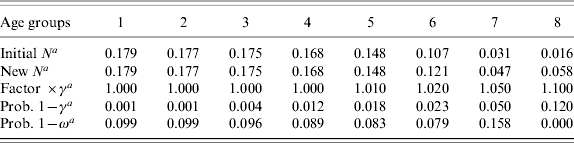
Becoming older in our model means that the mass of people in their eighties becomes larger because more of the younger agents make it to their eighties. Living longer means that the life-time horizon gets longer. To implement the scenario, we raise the survival rates of age groups 5 to 8 as in Table 4 but keep the expected duration in each age group constant. The mortality rates 1−γa decline, which necessarily implies that a larger fraction of this group moves to the next one, instead of dying. Since the last group becomes less mortal, 1−γ8 falling from 0.2 to 0.12, expected duration in that group rises from 5 to (1−γ8)−1=8.3 years. The representative agent lives longer, namely 93.3 instead of 90 years. This corresponds to the aging scenario in Kalemli-Ozcan et al. (Reference Kalemli-Ozcan, Ryder and Weil2000) who discuss the implications of longevity in a model with a single mortality rate.
Aging and life expectancy
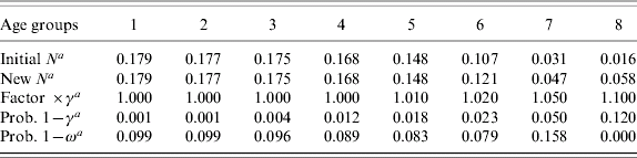
Note: 1−γa mortality rate, 1−ωa probability of aging.
In the simulations, we start with a net foreign debt–GDP ratio calibrated to equal 0.25. In a small open economy, the real interest rate is fixed on world markets. Any imbalance between domestic savings and investment is thus reflected in a change in the net foreign asset position.Footnote 10
6.1 Population aging
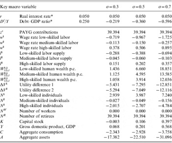
The effects of population aging are summarized in Table 7 in the appendix. Even though the interest rate remains constant, the ratio between capital and the three different kinds of labor varies due to the nested CES-production technology described in Section 8.4. Aging results in a larger number of old people. In the absence of an offsetting decline in fertility, the mass of younger age groups remains unchanged, leading to a constant workforce. By assumption, the increased number of retirees increases required PAYG contributions by almost 40%. These crowd out private savings and aggregate asset holdings by households (−22.5% in the baseline case), which is reflected in a sharp decrease in net foreign assets. The projected fall in savings is also found by Miles (Reference Miles1999). Since PAYG contributions are lump-sum, there is no direct effect on wages and labor supply; GDP and the capital stock remain virtually unchanged. The slight increase in the capital stock induces a rise of wage differentials. The decrease in the utility differences between skill classes, which leads to a fall in educational attainment, is due to the increase in total pension benefits, which is relatively more important for unskilled labor. The resulting decrease of the high-skilled workforce increases the wage of skilled labor, which leads to an increase in individual labor supply of skilled workers. Human wealth, consisting of human capital and social security wealth, increases in all skill classes; the increase in total pension entitlements benefits low-skilled workers most, however, because the proportional increase in PAYG contributions affects them least relative to their total wealth.
6.2 Population aging and postponed retirement
In the second simulation, we consider an increase in the retirement age by two years. The third simulation will then merge the two first scenarios in order to evaluate the combined effect of aging and pension reform. For simplicity, we impose the postponement of retirement exogenously.
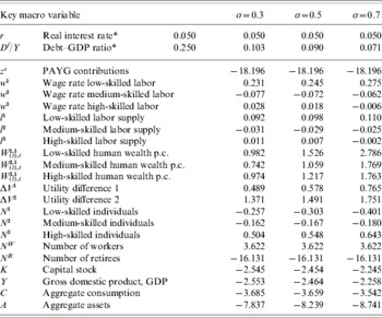
A two-year postponement of retirement increases the workforce by 3.6%, while reducing the number of retirees by 16.1% (cf. Table 8 in the appendix). Keeping per-capita pension benefits constant, this results in a decrease in necessary PAYG contributions by 18.2%. Postponed retirement reduces the need for individual pension savings, so that asset holdings decrease by 8.2% in the baseline case. Postponed retirement prolongs the redemption period of investments in human capital, such that the utility difference between skilled and unskilled workers increases and educational attainment rises. Also, education at the intensive margin rises due to a longer redemption period of human capital investments. This is reflected in increased levels of human wealth. These results are perfectly in line with the comparative static effects found in Section 4.4 in the context of the illustrative model. In a similar experiment, Trostel (Reference Trostel1993) finds that the level of the income tax rate decisively affects human capital accumulation.Footnote 11 However, his quantitative results are not directly comparable to ours, since an increase in the income tax rate affects both the costs and benefits of investment in human capital, while, in our setting, postponed retirement only affects the benefit side of the education decision.
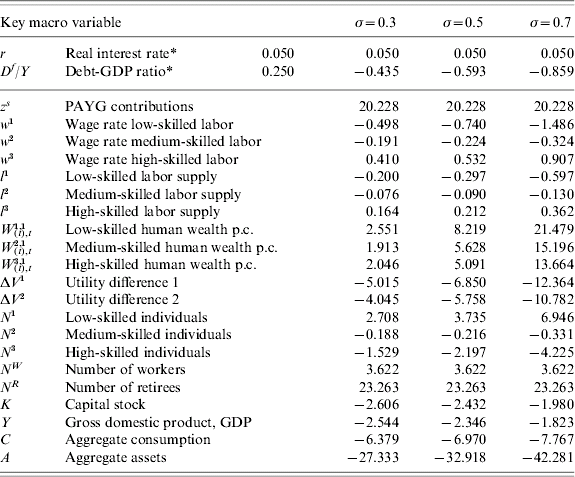
The third simulation considers a scenario on top of population aging with potentially less severe economic consequences due to the postponement of retirement (cf. Table 9 in the appendix).Footnote 12 Part of the overall population increase accrues now to workers. Therefore, PAYG payments increase only by 20.2%, compared with 40% in the case of constant retirement. Also, the adverse skill choice effects are somewhat mitigated. However, since postponed retirement reduces the time individuals stay in retirement, there is less need for individual savings to augment consumption possibilities at later ages. Therefore, the decrease in asset holdings due to aging is even aggravated. This effect is a result, however, of the low level of PAYG payments. Higher benefit levels would lessen the need for private savings and therefore dampen the adverse effect of postponed retirement on asset holdings. The disproportionate increase of low-skilled individuals' human wealth lowers educational attainment and thereby the capital stock via the complementarity between capital and high-skilled labor, as discussed in Section 4. Together, they depress GDP by 2.3% in the baseline simulation. Hence, considering individual saving effects, and allowing for capital–skill complementarity in production, results in postponed retirement not being appropriate to mitigate the adverse economic effects of population aging.
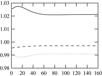
Figure 7 displays the discrete skill choice over time. The solid line depicts the choice for high-skilled labor relative to the initial steady state. The dashed and dotted lines show medium- and low-skilled labor, respectively.
Discrete skill choice over time

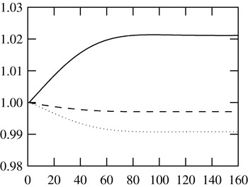
Reduced utility differences between different skill classes sharply decrease educational attainment. In the long run, wages adjust, and attainment returns towards its initial level. This is exactly the effect shown in 4 in the context of the stylized model. The relative size of the three skill groups evolves according to the inflows of individuals into these groups, as displayed in Figure 8. Again, the solid line depicts high-skilled labor relative to the initial steady state. The dashed and dotted lines show medium- and low-skilled labor, respectively.
The size of the three skill classes

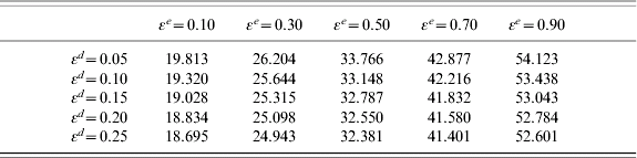
The key model parameters are the elasticity of substitution between capital and the three different kinds of labor as well as the education choice parameters at the extensive and intensive margins. We check the robustness of our results and the importance of the educational decision margins by varying the values of these parameters. Table 5 displays the sensitivity of the effect of aging and postponed retirement on aggregate human wealth. Overall, human wealth increases due to the prolongation of the redemption period, which yields investments in human capital more profitable at any stage of the life cycle.
Sensitivity of human wealth to education parameters
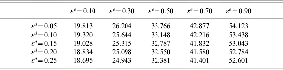
As economic intuition suggests, total human wealth reacts more the higher the training elasticity with respect to training returns εe. However, its responsiveness decreases in the semi-elasticity of the discrete skill choice decision. This is due to the negative reaction of educational attainment to aging and postponed retirement, which partly offsets the positive effect on intensive human capital formation.
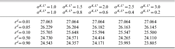
Table 6 shows the sensitivity of human wealth to the elasticities of substitution between capital and low-skilled labor,

, and between capital and high-skilled labor,

, which determine the degree of complementarity between capital and skill. The larger the difference

, the larger is the complementarity. In the first column, all elasticities of substitution between capital and labor are equal to unity, as for example with a Cobb–Douglas production technology. As in Table 5, an increase in the skill choice semi-elasticity reduces the response of human wealth to aging and postponed retirement due to lower attainment. An increase in capital–skill complementarity affects the response of human wealth to aging and postponed retirement only to the degree that individuals actually adapt their skill choice to labor market conditions; i.e., with εd close to zero, capital–skill complementarity is of little economic importance.
Sensitivity of human wealth to capital–skill complementarity
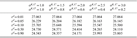

, εe = 0.3.
7 Conclusion
In this paper, we study the importance of education and human capital formation in a macroeconomic context. We apply the concept of probabilistic aging with endogenous discrete skill choice to analyze the economic impact of aging during demographic transition. The model setting allows for an appraisal of inter- and intragenerational distribution effects by considering eight age groups and three skill classes with endogenous human capital accumulation at the extensive and intensive margins. The empirically well-established complementarity between capital and skilled labor is embraced in a nested CES production technology. Simulating the effect of aging on key macro variables, we find that the remunerations of labor in different skill classes and accordingly their size are very differently affected. In a small open economy, where the interest rate is tied to international capital markets, GDP contracts due to decreased labor supply as a result of lower net wages and the adverse effect on educational attainment. Postponed retirement solves this problem partially by prolonging the redemption period of investments in human capital and thereby inducing higher extensive and intensive education. However, it introduces a new one: decreased private savings due to a lower need for funded old-age benefits.
8 Appendix
This first appendix outlines the concept of probabilistic aging as in Grafenhofer et al. (Reference Grafenhofer, Jaag, Keuschnigg and Keuschnigg2005), which allows for the possibility that an individual keeps her individual characteristics, such as age and productivity in the next time period, but also that she may be struck by sudden death. In the second appendix, we describe individual life-cycle optimization with respect to labor supply and intensive education. The third appendix contains a discussion of the extensive education decision. In the fourth appendix, we present the production part of the model with capital–skill complementarity in the production technology. The fifth appendix contains the simulation results in table form.
8.1 Probabilistic aging
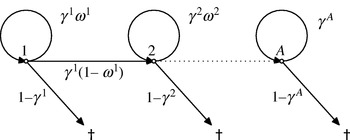
In order to reproduce realistic wage profiles, individuals must undergo some kind of aging. To preserve aggregability, aging is absent in Blanchard-style models of ‘perpetual youth’ with overlapping generations. Since we are interested in modeling life-cycle wage profiles in the context of an OLG model of the Blanchard style, while still being able to find closed-form aggregate solutions, we use the concept of probabilistic aging to model aging as shown in Figure 9. In this section, we concentrate on individual decisions once their skill level s is determined and fixed. We therefore temporarily drop superscript s. Each individual is a member of one of A age or productivity groups a∊{1, …, A}. Individuals are born in age group a=1 as workers. The affiliation of a variable at time t to an individual currently belonging to age group a is denoted by (·)ta.
Aging and mortality hazard of individuals in the model

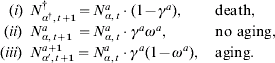
To model demographics, we allow for mortality among all age groups. When an individual with an arbitrarily given life-cycle history plans for the next period, she faces the risk of aging and dying (cf. Figure 9). She must thus reckon with three possible events: (i) she dies with probability 1−γa; (ii) she survives without aging and remains in the same age group with probability γaωa, and (iii) she survives and ages and belongs to age group a+1 next period with probability γa (1−ωa). Individuals in the last age group have exhausted the aging process and remain in this group with probability one, ωA=1. They may either survive with probability γA within group A or die with probability 1−γA. In this setting, time passes faster than age, i.e. individuals normally stay in the same age group for several periods. The last age group behaves according to the mortality and demographic assumptions of Blanchard's perpetual youth model.
The number of agents at date t, in state of life a and with aging history α is given by N aα,t. Within this group, agents are identical up to their skill level and asset holdings and face the same independent probability of moving to one of the alternative states. With stochastically independent risks, the law of large numbers implies that the above-stated individual probabilities correspond to the fraction of people that are subject to the respective events. Consequently, the group is divided into three subgroups next period: (i) those who die, (ii) those who survive within the same age group a, and (iii) those who are hit by an aging event, switch to the next higher age group. The age group and the biography α remains unchanged in case (ii) while switching to the next higher age group a+1 in case (iii) adds another event in a person's life cycle history α and thereby results in a new biography α′:
Since the characteristics of people such as their earnings potential differ across age groups, an agent's consumption, assets, and other economic variables will generally depend on her particular life cycle history. For example, assets depend on the agent's past earnings history which, in turn, is linked to her aging trajectory. To keep track of the population's heterogeneity, one must thus identify each agent by her age group as well as her aging biography α which also includes the date of birth. An agent's life cycle history is her biography of aging events that have happened since birth. At date t, the set of possible histories of a household that belongs to age group a is

A particular life-cycle history is represented by a vector α∊ℵta. The element αi, i∊{1, …, a}, denotes the date at which the household who was formerly in age group i−1 became a member of group i. In denoting the unborn by a virtual age group zero, the element α1 lists the date of birth when an agent switches from the group of the unborn to the first age group. We say that a member of group a=1 aged only once with no further aging since birth. Nevertheless, different persons of the first age group are heterogeneous since they were born at different moments in the past. The set of possible biographies is then ℵt1={(α1):t⩾α1}. With this notation, the vectors α describing the biography of people in group a have a elements since such persons have aged a times in total.
The individual biographies are updated when a person is subject to an aging event. Suppose a person is in age group a−1 and is identified by a given biography α=(α1, …, αa−1). When the next aging event occurs in period t, she arrives in group a next period. Her biography is appended by the entry t+1 and will thus read (α1, …, αa−1, t+1). Accordingly, the set ℵta of biographies of age group a will be augmented next period by all the biographies α′∊ℵta−1×(t+1) that have t+1 as their last entry and refer to people who currently switch from group a−1 to a. Hence

Result 1. With the number of individuals in age group a given by

(a) the aggregate law of motion for age group 1<a⩽A is
(16)
(b) age group 1 evolves according to
(17)(c total population grows by
(18)



Proof Cf. Grafenhofer et al. (Reference Grafenhofer, Jaag, Keuschnigg and Keuschnigg2005).
8.2 Life cycle optimization
In different stages of the life cycle, the individuals' choice set varies, such that intertemporal optimization differs across age groups. As a representative case, we sketch the problem of individuals belonging to the last working age group. The analogous problem of other age groups is detailed in Jaag et al. (Reference Jaag, Keuschnigg and Keuschnigg2005).
Individuals are working with probability πt and retired with probability 1−πt. Workers use time for post-school training e and hours worked l, giving rise to effort costs ϕe and ϕl for education and work, respectively, multiplied by skill θ. State variables are assets A and skills θ. Preferences are assumed additively separable in consumption C and job-related efforts. The per-capita Bellman equation for maximizing expected life-time utility isFootnote 13



With R denoting the real interest factor and G an exogenous growth rate, workers accumulate assets and skills according to


where

is an exogenous transfer or a lump-sum tax to workers,

a transfer to retirees, δS skill depreciation, and F(·) is the intensive skill production function, assumed to be linear homogenous. Switching to the next age group implies θα′,t+1a+1=θα,t+1a and A α′,t+1a+1=A α,t+1a. Net labor income is given by

where w ta is the wage per efficiency or productivity unit per hour, θα,ta is the agent's productivity (skill) resulting from past training, and I α,ta is physical investment in training (books, computers, teachers). We assume that this is a government provided rival good, and thus exogenously controlled. It is supplied at the same amount for all per capita, I α,ta=I t, and the cost of it is charged to private agents, giving rise to private spending I t.
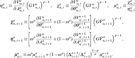
It is convenient to define the shadow prices ηα,ta of assets and χα,ta of skills
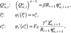
The optimality conditions for (19) subject to (22)/(23) are
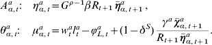
where F E denotes the partial derivatives of F with respect to e. The envelope theorem yields
Result 2. Consumption Q α,taand indirect utility V α,taare

Ωt+1aaugments the interest rate R t+1, accounting for the expected finiteness of life, Δtais the inverse of the marginal propensity to consume, H is human capital, and S is social security wealth.
Proof Cf. Jaag et al. (Reference Jaag, Keuschnigg and Keuschnigg2005), proposition 3.□
Physical investment in education I being determined exogenously, there are private rents on education yr a, which derive from the inframargial effort and the non-optimal supply of I.
Result 3. Human capital can be written as shadow price times accumulated skills

where
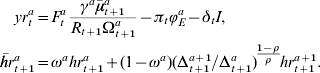
Proof Cf. Jaag et al. (Reference Jaag, Keuschnigg and Keuschnigg2005), equation (28).□
8.3 Discrete skill choice
At the beginning of their life cycle, individuals choose their skill level. For simplicity, we assume this education to be instantaneous with no time being consumed.Footnote 14 We distinguish several discrete skill classes and introduce an upper index s∊{1, …, S} to identify these groups (e.g. high, medium, and low skilled in case of three groups). The structure of individual decisions in the preceding section is identical for all skill classes. Indirect utility of a new agent born at date t with skill s is V (t),ts,1. This agent necessarily belongs to age group 1 and has history α1=t. Let ϕvs>0 be the incremental education effort cost that an agent with skill s needs to spend to obtain skill s+1. The discrete skill choice at the beginning of the life cycle is

To obtain a determinate education decision, we must assume heterogeneity of agents with respect to ability, which is inversely related to the index

.
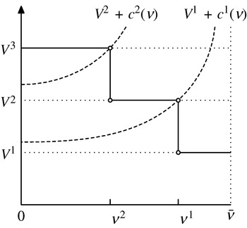
The discrete skill choice is most easily found by starting with the lowest skill class s=1 and asking whether it pays to obtain the next higher degree. Following this procedure, an agent with skill s acquires the incremental education to obtain degree s+1 if the following inequality derived from (25) holds: V (t),ts+1,1>V (t),ts,1+ϕνs(ν). For high-cost, low-ability persons, it is eventually not worthwhile anymore to incur the incremental education cost. Hence, there exists a critical agent v s who is just indifferent between degrees s and s+1

Since education cost increases in v, agents with lower ability v>v s and higher cost remain with skill s. Figure 10 illustrates.
Discrete skill choice with three skill classes

New agents are distributed by the cumulative distribution function Γ(v). Of all N (t),t1 new agents in period t, a share p ts chooses skill group s where 1 gives the lowest and S the highest skill group

The educational choice is open only to new households while older ones are locked into their previously chosen skill group. Hence, the law of motion for the number of individuals in age group 1 with skill level s is

Assume a uniform distribution of the population v~U (0, 1) which implies Γ(ν)s=νs. We specify the cost of education to be

This specification implies a semi-elasticity εd of the education decision with respect to

, i.e.

. When life-time utility of skill s+1 increases relative to s, the critical value νs increases and the share of skill group s in the new cohort declines by dνs.
8.4 Capital–skill complementarity in production
In our model, we allow for differentiated labor in the production function. As opposed to Heckman et al. (Reference Heckman, Lochner and Taber1998), Blundell and Bond (Reference Blundell and Bond2000), and Blundell et al. (Reference Blundell, Dias and Meghir2003), we explicitly allow for capital–skill complementarity and hence for a non-constant share of capital in production. There are several ways of nesting the differentiated production factors within a CES function, of which six allow for full capital–skill complementarity. With a monotonous ordering of labor inputs according to their skill level, there are two nestings
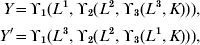
where ϒ1, ϒ2, ϒ3 are CES aggregators. Y′ implies the elasticity of substitution between L 3 and K to be the same as between L 1 and L 3 by the symmetry restrictions of the CES functional form. This is at odds with factor elasticity estimates, which suggest that the substitution elasticity between skilled labor and unskilled labor is higher than the substitution elasticity between skilled labor and capital (cf. Hamermesh, Reference Hamermesh1993; Krusell et al., Reference Krusell, Ohanian, Rios-Rull and Violante2000). Hence, we choose Y which does not seem to be at variance with elasticity estimates. This ordering of the CES nesting also conforms with the functional form chosen by Duffy et al. (Reference Duffy, Papageorgiou and Perez-Sebastian2004).
For the simulations, we use a production function with three kinds of labor and capital as inputs of the form (cf. Figure 11)

The most aggregate nest is final output Y, which consists of unskilled labor L 1, and a quantity Y 2, which is the output of the next subnest and itself consists of medium-skilled labor L 2 and a composite Y 3. This last quantity is a composite of high-skilled labor L 3 and capital K. The parameters κ1, κ2, κ3 are related to substitution elasticities, and a 1, a 2, a 3 are distribution parameters. The technology is thus
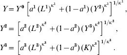
Production technology with three-level nested CES structure

Note that only one type of labor enters at each level of nesting. The technology can be characterized by the price elasticity of demand for the input factors. Let w s be the unit price of labor of type s and c s the unit cost of output of level s, i.e. c s=F Ls⋅L s/Y s+c s+1⋅Y s+1/Y s. The cost-minimization problem at each level s is

We get input demands at level s

By forward substitution, total compensated demand for labor on aggregation level s∊{1, 2, 3}, L s, is given by

By Shephard's lemma, the derivative of total cost with respect to w i equals the demand for input factor i
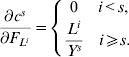
Therefore, the compensated own-price elasticity of demand for labor s is

Let k∊{i, j} denote the deepest price aggregate which contains both F L i and F L j.Taking into account the impact of F L i on c j⩽k, the cross price elasticity is given by

In analogy, the cross price elasticity between labor L s and capital K is

where w K is the cost per unit of capital.
The key parameters to consider in the calibration of the production side of the model are the elasticities of substitution between input factors. For production functions with more than two inputs, there are multiple possible definitions for the elasticity of substitution between pairs of input. The most commonly used is the Allen–Uzawa partial elasticity of substitution which measures the percentage change in the ratio of two inputs in response to a change in the ratio of the two input prices, holding all other prices – but not all other inputs – and the output quantity constant. This measure is widely used in the empirical literature, e.g. by Sato (1967), Griliches (Reference Griliches1969), and Goldin and Katz (Reference Goldin and Katz1998). The Allen–Uzawa elasticity of substitution is
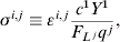
where q j is the quantity of input good j.Footnote 15 Denote by k the deepest aggregate containing both inputs i and j. In the production function with the nest at level 1 producing final output, the elasticities of substitution between any two input factors i and j write as

where c n is the unit cost of a nest at level n and

Note that the elasticity of substitution between i and j is independent of the subnest elasticity in all nests s>k. Applying the concept of capital–skill complementarity implies in the setting of our production technology thatFootnote 16

The relative income shares of the three kinds of labor and capital are known from data. The elasticities of substitution between capital and skilled/unskilled labor are taken from the empirical literature. Using three types of labor, it is clear that high-skilled labor is even more complementary with capital than skilled labor in the literature dealing with two kinds of labor only. Hence, we correct the respective elasticities of substitution between capital and skilled/unskilled labor accordingly. The values of σ1, σ2, σ3 are computed from (28) recursively
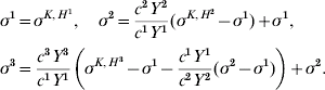
Using

we get κ1=0.375, κ2=0.045, κ3=−0.238 (cf. Figure 11). From national accounting we know the income shares of the different production factors. Taking these into account, we can calibrate the distribution coefficients a 1=0.163, a 2=0.365, a 3=0.288.
8.5 Simulation results
Long-run impact of aging on key macro variables in percentage changes relative to initial steady state

Notes: Pension benefits p.c. and public consumption p.c. constant; W α,ts,a =H α,ts,a +S α,ts,a ; * absolute values, initial values in first column.
Long-run impact of a two-year retirement postponement on key macro variables in percentage changes relative to initial steady state

Notes: Pension benefits p.c. and public consumption p.c. constant; W α,ts,a =H α,ts,a +S α,ts,a ; * absolute values, initial values in first column.
Long-run impact of aging and postponed retirement on key macro variables in percentage changes relative to initial steady state
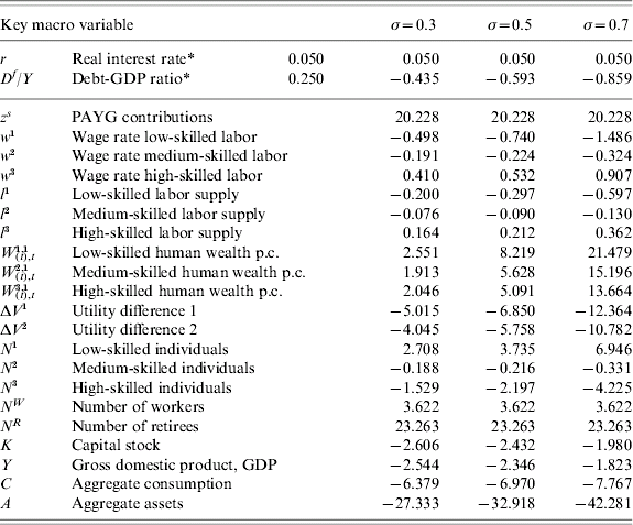
Notes: Pension benefits p.c. and public consumption p.c. constant; W α,ts,a =H α,ts,a +S α,ts,a ; * absolute values, initial values in first column.