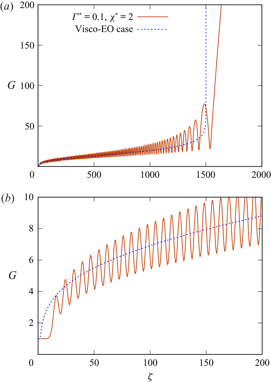
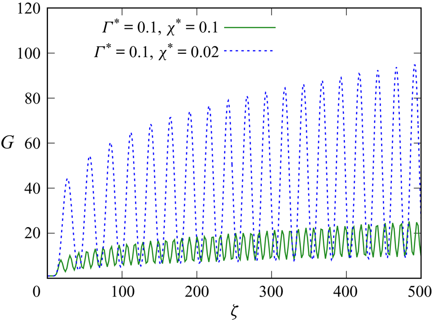
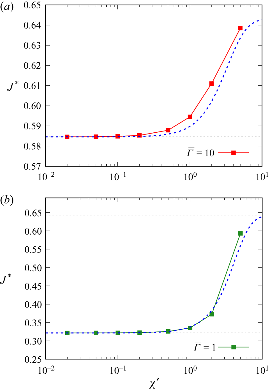
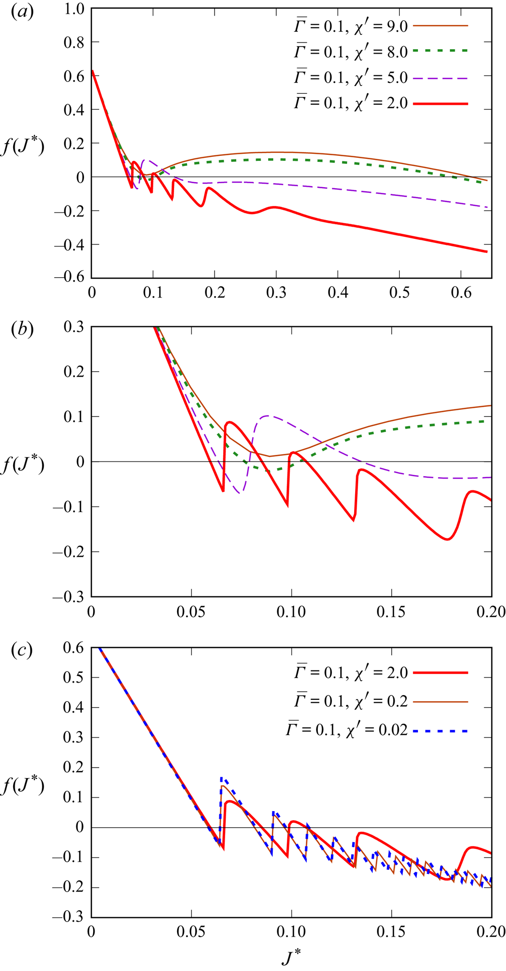
1. Introduction
The advance of a non-aqueous dispersed phase into a capillary channel initially containing a continuous aqueous phase (a classical fluid mechanics problem solved by Bretherton Reference Bretherton1961) is a situation occurring in a number of processes of physical or engineering interest. These include micro-fluidic emulsification/emulsion processing (Anna, Bontoux & Stone Reference Anna, Bontoux and Stone2003), droplet encapsulation for biomedical applications (including drug delivery) (Teh et al. Reference Teh, Lin, Hung and Lee2008), micro-fluidic reactors (Teh et al. Reference Teh, Lin, Hung and Lee2008) and decontamination of soils (Geraud et al. Reference Geraud, Jones, Cantat, Dollet and Meheust2016). The particular process of interest in the present work is waterflooding in oil recovery (Willhite Reference Willhite1986). During this process, water is injected under pressure into a porous oil bearing rock, so that oil, that is initially trapped within droplets in capillary pores in the rock, will be driven out through the rock's network of pores, and then recovered.
The oil droplet as it moves along a pore displaces the aqueous phase ahead of it, and in turn is displaced by the aqueous phase behind it. Forces relevant to droplet displacement through capillary channels include surface tension/capillary forces and viscous forces. These need not, however, be the only forces present. It is possible that the droplet surface or the capillary surface (or both) can be charged (Lager et al. Reference Lager, Webb, Black, Singleton and Sorbie2008). Thus, electro-static, or more specifically electro-osmotic, forces (Yang, Fu & Hwang Reference Yang, Fu and Hwang2001; Waghmare & Mitra Reference Waghmare and Mitra2008) can be relevant. Moreover, the charge state of the surfaces (and hence the electro-osmotic forces produced) can be manipulated via changing ion concentrations in the bulk aqueous phase, which determines the extent of ion adsorption onto surfaces (Wilmott, Breward & Chapman Reference Wilmott, Breward and Chapman2018). Indeed, it has been observed that the performance of waterflooding operations for oil recovery can be sensitive to salinity levels in the water used for the flood (McGuire et al. Reference McGuire, Chatham, Paskvan, Sommer and Carini2005; Lager et al. Reference Lager, Webb, Black, Singleton and Sorbie2008; Lee et al. Reference Lee, Webb, Collins, Lager, Clarke, O'Sullivan, Routh and Wang2010; Rezaei Doust, Puntervold & Austad Reference Rezaei Doust, Puntervold and Austad2011): high salinity floods (e.g. with the composition of sea water) often perform less well in oil recovery terms than lower salinity floods (up to a couple of orders of magnitude less saline). The difference in behaviour between high and low salinity floods has been postulated to be due to the difference in electro-osmotic forces between these different situations (Lager et al. Reference Lager, Webb, Black, Singleton and Sorbie2008; Wilmott et al. Reference Wilmott, Breward and Chapman2018; Grassia Reference Grassia2019). Although a full predictive model of how to optimise waterflood performance by manipulation of salinity has yet to be developed, it is clear that enhancing understanding of how electro-osmotic effects influence displacement of an oil droplet along a capillary represents a step towards a predictive model. Obtaining such understanding is what the present work sets out to achieve, building on work in two recent publications (Wilmott et al. Reference Wilmott, Breward and Chapman2018; Grassia Reference Grassia2019). In what remains of this section, we review what is known (and also what is not yet known) about the behaviour of a moving droplet in a capillary pore, both with and without electrical charges.
1.1. Droplet moving through a capillary: uncharged case
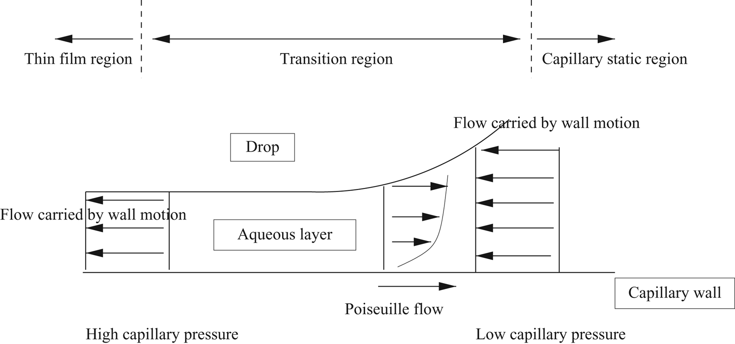
It is known (Bretherton Reference Bretherton1961) that there are uniformly curved capillary static regions at the ends of the droplet, whilst away from the ends, there is a thin film region, in which the droplet is separated from the capillary wall by a thin aqueous layer. A thicker aqueous film or ‘transition region’ separates the thin film region from the capillary static regions at the ends, see figure 1, which focusses specifically on the front of the droplet.
View of a non-aqueous droplet that is surrounded by aqueous liquid and moving along a capillary. The view focusses on just part of the droplet near its front end and is in the frame of reference of the droplet, such that there is net motion of aqueous liquid to the left. In this view, a transition region joins the thin film region (left) to the capillary static region (right). Leftward flows are carried by the moving capillary wall at each location, but since the net leftward flow is position independent, a rightward Poiseuille flow is required in the thicker parts of the film. This is typically driven by a capillary pressure gradient. Capillary pressure decreases in the direction that aqueous layer thickness increases.

Adopting a frame of reference in which the droplet boundary is stationary but the capillary channel walls are moving, a continuity equation can be obtained for the liquid flow along the aqueous phase. This equation (presented later, see § 2.2) states that the leftward flow in the thin film (carried by the moving wall) must be balanced in the thicker film region by a larger leftward flow (again carried by the moving wall) but offset by a rightward Poiseuille flow, again see figure 1. In the absence of any electrical charge effects (Bretherton Reference Bretherton1961), the Poiseuille flow in the thicker film is driven by a capillary pressure gradient. The capillary pressure depends on the interface curvature. At the front of the droplet, see figure 1, capillary pressure is always negative relative to the pressure in the droplet itself. Moreover, pressure in the aqueous phase is highest (i.e. least negative) in the thin film region (where the film is becoming flat) and lowest (i.e. most negative) in the uniformly curved capillary static region. In figure 1, the pressure gradient therefore drives Poiseuille flow from left to right (as we expect), away from the thin film, which is what ensures the thin film really is thin. Pressure thereby decreases in the direction in which film thickness increases.
The situation at the rear of the drop is more complex (Bretherton Reference Bretherton1961). As the film thickens towards a capillary static region at the rear, a significant flux of fluid is advected along by the wall, and this must be opposed by a capillary pressure gradient (itself associated with a gradient of film curvature) that drives a Poiseuille flow towards (not away from) the thin film region. The direction in which capillary pressure in the aqueous film decreases is now opposed to the direction in which film thickness increases (a contrast from figure 1). This change in sign in the relation between capillary pressure gradient and gradient of film thickness when contrasting the rear of the drop with the front, turns out to cause the film thickness at the rear to become oscillatory with position (Wong, Radke & Morris Reference Wong, Radke and Morris1995a,Reference Wong, Radke and Morrisb; Wilmott et al. Reference Wilmott, Breward and Chapman2018), whereas at the front end it is monotonic.
1.2. Charged droplet moving through a charged capillary: repulsive case
Extensions to the classical system of Bretherton (Reference Bretherton1961) to incorporate the effect of electrostatic potentials have been considered by a number of authors (Teletzke, Davis & Scriven Reference Teletzke, Davis and Scriven1987, Reference Teletzke, Davis and Scriven1988; Krechetnikov & Homsy Reference Krechetnikov and Homsy2005; Wilmott et al. Reference Wilmott, Breward and Chapman2018; Grassia Reference Grassia2019). In a typical situation (Grassia Reference Grassia2019) in which the capillary wall and droplet have like charges, we see a large electro-osmotic repulsion in the thin film region (the repulsive force can scale with an inverse square law of distance) but no electro-osmotic effects in the capillary static region (since charges are screened in that latter region (Wright Reference Wright2007) according to Debye–Hückel theory). Expressing this in terms of electro-osmotic disjoining tension (tension is the negative of pressure), implies (Wilmott et al. Reference Wilmott, Breward and Chapman2018) a large (and positive) electro-osmotic tension for a thin film but a zero electro-osmotic tension in the capillary static region. Taking gradients of pressures and/or tensions along the droplet, we deduce that the sign of the capillary pressure gradient (at the front of the drop, as per the sketch in figure 1) matches that of the electro-osmotic tension gradient, or equivalently the sign of the electro-osmotic pressure gradient opposes that of the capillary pressure gradient.
It follows that, whereas the capillary pressure gradient generates Poiseuille flows that make films thinner (as noted above), repulsive electro-osmotic interactions generate opposing Poiseuille flows tending to thicken them. In an extreme case, films thicken to the point in which capillary and electro-osmotic pressure gradients cancel each other out (Grassia Reference Grassia2019). A so-called augmented Young–Laplace state (Teletzke et al. Reference Teletzke, Davis and Scriven1988) is then reached in which films are found to be much thicker than their classical counterparts from Bretherton (Reference Bretherton1961), and as a result viscous forces cease to play a role (shear rates and hence associated viscous forces only being significant in thin films).
The above arguments assume repulsive electro-static interactions below the charge screening distance. It is possible, however, to consider a system (Grassia Reference Grassia2019) in which the electro-static interactions below the charge screening distance instead are attractive conjoining forces: this is considered next.
1.3. Charged droplet moving through a charged capillary: attractive case
In the attractive case, and also still focussing on the front of the drop as per figure 1, the capillary pressure field and the electro-osmotic pressure field, rather than opposing one another, should co-operate. This will increase the net rightward Poiseuille flow driven by these combined pressures, which will then offset even more of the leftward flow carried by the moving capillary wall. The result (Grassia Reference Grassia2019) is that, for attractive electro-osmotic interactions, the thin film will actually reduce in thickness compared to the classical case of Bretherton (Reference Bretherton1961), not increase in thickness, as happens for repulsive interactions.
When the electro-osmotic and capillary pressure co-operate, rather than compete, it is not possible for the gradient of one to cancel out the gradient of the other, as is required to achieve an augmented Young–Laplace state. A question that we address in what follows is whether the electro-osmotic terms can ever become sufficiently strong as to replace the capillary terms entirely. We will explore whether, for attractive electro-osmotic interactions, the full system governed by capillary, viscous and electro-osmotic forces, can ever be replaced by an approximate system in which solely viscous and electro-osmotic forces are retained. By way of contrast, we know already that there is a capillary, viscous limiting case (the classical case of Bretherton Reference Bretherton1961) as well as a capillary, electro-osmotic limit (the so-called augmented Young–Laplace limit Teletzke et al. Reference Teletzke, Davis and Scriven1988 mentioned earlier, which is certainly realised for repulsive electro-osmotic interactions).
We will find for attractive electro-osmotic interactions that a visco-electro-osmotic limiting case is not possible uniformly over the entire length of the droplet: we can never eliminate the aforementioned capillary static regions at the ends. However, we will find that a visco-electro-osmotic limiting case may apply over part of the droplet, specifically over a significant part of the aforementioned ‘transition region’. That said, we will also find that the droplet often adjusts itself, in particular it adjusts the thickness of the thin film region and the shape of the interface along the transition region, in such a fashion that nominally weak capillary effects manage to retain importance. As we will see, one way that the transition region adjusts to incorporate capillarity is for its shape to become oscillatory with position. A further consequence turns out to be that there can be multiple solutions for the drop shape, with different thicknesses of the thin film region. Note, however, that while the present work identifies multiple solutions, it does not interrogate which of them might be stable.
The rest of this work is laid out as follows. Section 2 reviews the model and governing equations, after which § 3 highlights limiting cases of interest that are analysed further. Section 4 presents results, comparing them with predictions made in § 3. Finally § 5 offers conclusions.
2. Model and governing equations
This section, which follows the development already outlined in Wilmott et al. (Reference Wilmott, Breward and Chapman2018) and Grassia (Reference Grassia2019), is laid out as follows. In § 2.1 we specify in physical terms the model system under consideration, presenting governing equations in §§ 2.2 and 2.3. After that, we focus specifically on the nature of the electro-osmotic terms in §§ 2.4 and 2.5. Then in § 2.6 we identify the domain of parameter values to be studied. A linearisation of the governing equations is presented in § 2.7. The linearisation allows us to initiate a numerical scheme, which once initiated, can extend even to regions in which the solutions exhibit nonlinearity: the numerical scheme itself is presented in § 2.8. Readers already familiar with the above mentioned material from Wilmott et al. (Reference Wilmott, Breward and Chapman2018) and Grassia (Reference Grassia2019) may wish to skip directly to § 3.
2.1. Model system under consideration
We consider (Bretherton Reference Bretherton1961) a non-aqueous droplet advancing into a capillary channel initially filled with an aqueous phase. In what follows we study a two-dimensional (2-D) planar system, although a three-dimensional axisymmetric system is qualitatively similar. In this 2-D system, aqueous films are formed symmetrically on both upper and lower channel walls, so consideration is restricted to just half the width of the channel.
Along the length of the droplet, the system is divided into different regions (see figure 1). As mentioned earlier, at either end of the droplet, there will be a capillary static region where the droplet surface is uniformly curved, with an a priori known curvature, fixed by the half-width of the capillary channel. Far from the ends, there will be a thin film region, in which the aqueous film is much thinner than the channel half-width: the thickness is, however, a priori unknown. There will also be so-called transition regions (Bretherton Reference Bretherton1961) joining the thin film region to the capillary static regions, and these are what we aim to compute. We focus here on the transition region at the front of the droplet rather than at the rear. Whereas the thickness tends to oscillate in a non-monotonic fashion at the rear, at the front of the droplet conventionally (at least in the case of Bretherton Reference Bretherton1961), thickness changes monotonically with position. A contribution of the present work, however, already mentioned in § 1.3, will be to demonstrate that under a special set of circumstances (a system augmented by attractive electro-osmotic tensions) layer thickness can be non-monotonic with position even at the front of the droplet. The result that adding attractive electro-osmotic tensions can turn an originally non-oscillatory profile into an oscillatory one is striking, hence the focus on the front of the droplet here. Governing equations for the system are considered next.
2.2. Governing equations
The governing equation for how, within the transition region, the thickness  $h$ varies with distance
 $Z$ along the aqueous film is deduced as follows (Wilmott et al. Reference Wilmott, Breward and Chapman2018; Grassia Reference Grassia2019). Suppose the droplet is moving through a capillary channel at velocity
 $U$, or equivalently, in the reference frame of the droplet, suppose the capillary wall is moving at velocity
 $-U$ relative to the droplet. In the thin film region, supposing the film thickness is
 $h^{\ast }$, the flux of aqueous liquid carried by the moving wall is
 $-U h^{\ast }$. Outside the thin film region, i.e. in the transition region, the flux carried by the wall, however, is
 $-U h$. These two fluxes are unequal, yet in a steady state system, continuity demands that the total flux must be spatially uniform. Hence in the transition region there must be an additional flux, carried not by the moving wall, but instead (as mentioned earlier) driven by a Poiseuille flow associated with a net pressure gradient. For a pressure gradient
 $p_{Z}$ and aqueous layer viscosity
 $\mu$, the Poiseuille flow field is determined by imposing a no-slip condition on the capillary wall, and a shear stress free condition on the drop surface. Integrating this velocity field across the aqueous layer yields a flux
 $-p_{Z} \,h^{3}/(3\mu )$. Setting the pressure in the droplet itself to be zero, the pressure
 $p$ in the aqueous layer has both an electro-osmotic contribution and a capillary contribution, which we consider in turn.
The electro-osmotic contribution to  $p$ is usually written
 $-T_{\mathit {EO}}$ where
 $T_{\mathit {EO}}$ is an electro-osmotic tension. Here
 $T_{\mathit {EO}}$ is a function of the thickness
 $h$ of the aqueous layer, or more specifically of the ratio between the thickness
 $h$ of the layer and the thickness
 $\epsilon _{2}$ of an electrical double layer (Wright Reference Wright2007). The functional form
 $T_{\mathit {EO}}\equiv T_{\mathit {EO}}(h/\epsilon _{2})$ will be specified shortly (see §§ 2.4 and 2.5), although we note that in the problem to be studied here
 $T_{\mathit {EO}}$ turns out to be negative, i.e. there is a conjoining pressure, not a disjoining tension.
We note further that  $T_{\mathit {EO}}$ is negligible when
 $h\gg \epsilon _{2}$ on the grounds that charges are then screened, but may be quite significant when
 $h$ is of the order of
 $\epsilon _{2}$ or less, as charge screening does not then apply. The capillary contribution to
 $p$ is
 $-\gamma h_{ZZ}$, where
 $\gamma$ is interfacial tension and
 $h_{ZZ}$ is curvature. Here we suppose that
 $\gamma$ is constant and uniform, i.e. we neglect any effect of any effect of electric field upon interfacial tension.
Given the above two contributions to pressure, spatial uniformity of flux in the aqueous layer now demands  $- U \, h^{\ast } = - U \, h + {h^{3}}{/(3\mu )} (\gamma h_{ZZ} + T_{\mathit {EO}})_{Z}$.
We rearrange to obtain
 \begin{equation} \gamma h_{ZZZ} = 3\mu U \frac{h-h^{\ast}}{h^{3}} - (T_{\mathit{EO}}(h/\epsilon_{2}))_{h}\,h_{Z}. \end{equation}
In this equation, the left-hand side represents capillarity, while the first term on the right-hand side can be considered to represent viscous effects: although (2.1) is derived based on uniformity of fluid flux, ultimately it is owing to viscosity that a contribution to the fluid flux is carried along by the moving wall. Meanwhile the second term on the right-hand side represents electro-osmotic effects.
We now non-dimensionalise the above equation. Lengths (i.e.  $h$,
 $h^{\ast }$,
 $Z$ and
 $\epsilon _{2}$) are non-dimensionalised by the half-width
 $R$ of the capillary channel. A capillary number
 $Ca_{{B}}$ is defined as
 $\mu U/\gamma$.
The subscript ‘ ${B}$’ here reminds us that this is the definition of capillary number used by Bretherton (Reference Bretherton1961), not an alternate definition used by Wilmott et al. (Reference Wilmott, Breward and Chapman2018).
A dimensionless parameter  $\bar {\Gamma }$ is introduced that represents the relative importance of capillary and electro-osmotic terms, and is defined as (Grassia Reference Grassia2019)
 \begin{equation} \bar{\Gamma}=2\gamma \varepsilon_{w}/(R q^{2} s_{c}^{\ast\,2}),\end{equation}
with  $\gamma$ and
 $R$ being as defined above,
 $\varepsilon _{w}$ being electrical permittivity of the aqueous phase,
 $q$ being elementary electrical charge and
 $s_{c}^{\ast }$ being the density of charge adsorption sites on the capillary channel wall. Having defined
 $\bar {\Gamma }$, the electro-osmotic tension
 $T_{\mathit {EO}}$ can be non-dimensionalised on the scale
 $\gamma /(R \,\bar {\Gamma }) \equiv q^{2} s^{*\,2}_{c}/ (2 \varepsilon _{w})$.
Our analysis in what follows will be in terms of dimensionless rather than dimensional variables, but for compactness of notation we use the same symbols ( $h$,
 $h^{\ast }$,
 $Z$,
 $\epsilon _{2}$ and
 $T_{\mathit {EO}}$) to denote dimensionless variables from here on. Equation (2.1) now becomes
 \begin{equation} h_{ZZZ} = 3 Ca_{{B}} \frac{{h - h^{\ast}}}{h^{3}} - \frac{1}{\bar{\Gamma}}(T_{\mathit{EO}}(h/\epsilon_{2}))_{h} h_{Z}. \end{equation}
The contribution of Bretherton (Reference Bretherton1961) was to demonstrate, at least in the absence of any electro-osmotic effects ( $T_{\mathit {EO}}\equiv 0$), that the thickness and length of the transition region scaled respectively as
 $Ca_{{B}}^{2/3}$ and
 $Ca_{{B}}^{1/3}$. Since in problems of practical interest
 $Ca_{{B}}$ tends to be much smaller than unity (see e.g. the value of
 $Ca_{{B}}$ quoted in § 2.6.2 later on) the implication is that the transition region is both thinner and shorter than the half-width of the channel. Another consequence of this was that the droplet shape turned out to be relatively insensitive to the droplet-to-aqueous-layer viscosity ratio (Park & Homsy Reference Park and Homsy1984), as long as this ratio was smaller than
 $Ca_{{B}}^{-1/3}$ with
 $Ca_{{B}}\ll 1$ here. Effectively droplet viscosity is irrelevant here, and a droplet advancing into a capillary has the same shape as a bubble advancing into the same capillary at the same
 $Ca_{{B}}$ value.
2.2.1. Rescaling the governing equations
Despite (2.3) already being in dimensionless form, in view of the small thickness and length of the transition region predicted for the small  $Ca_{{B}}$ limit, Bretherton (Reference Bretherton1961) found it convenient to rescale it. The analysis proceeds by defining a rescaled film thickness in the thin film region
 $J^{\ast } = h^{\ast } / (3 Ca_\textrm {B})^{2/3}$, this value being a priori unknown. A rescaled coordinate along the film
 $\zeta = Z / ((3 Ca_\textrm {B})^{1/3}J^{\ast })$, and a rescaled thickness in the transition region
 $G = h/((3 Ca_\textrm {B})^{2/3} J^{\ast })$ are also defined. The problem to be considered here involves an extra dimensionless parameter, denoted
 $\chi '$, which is defined (Grassia Reference Grassia2019) as the ratio between the nominal film thickness based on the scaling of Bretherton (Reference Bretherton1961) and the Debye screening length
 \begin{equation} \chi'=(3Ca_{{B}}^{2/3})/\epsilon_{2}. \end{equation}
The larger the value of  $\chi '$, the more charges are screened. Equation (2.3) now becomes
 \begin{equation} G_{\zeta\zeta\zeta} = \frac{{G - 1}}{G^{3}} - \frac{1}{\Gamma^{\ast}} \left(T_{\mathit{EO}}(G\,\chi^{\ast}) \right)_{G} G_{\zeta}, \end{equation}
which now contains (as yet unknown) parameters  $\Gamma ^{\ast }$ and
 $\chi ^{\ast }$ defined as
 \begin{gather} \Gamma^{\ast} = \bar{\Gamma}/J^{\ast} \end{gather}
 \begin{gather} \chi^{\ast} = \chi' J^{\ast}. \end{gather}
Observe that  $h/\epsilon _{2}\equiv G\,\chi ^{\ast }$. Note also the curious fact via (2.6) that decreasing the film thickness
 $J^{\ast }$ actually decreases the factor
 $1/\Gamma ^{\ast }$, which in (2.5) governs the relative importance of electro-osmotic terms, despite the fact that electro-osmotic tensions themselves increase as the film thins. The reason is that the Poiseuille flow due to those electro-osmotic tensions decreases more rapidly with decreasing film thickness than the viscous flow carried along by the moving walls does. Likewise the Poiseuille flow due to the electro-osmotic tensions decreases more rapidly with decreasing film thickness than the Poiseuille flow associated with capillary pressures does: this follows from including a factor of
 $J^{\ast }$ in the conversion between the coordinates
 $Z$ and
 $\zeta$, effectively compressing the horizontal length scale, which favours capillary effects.
In the absence of electro-osmotic effects as per Bretherton (Reference Bretherton1961),  $T_{\mathit {EO}}\equiv 0$, and the rescaling given in (2.5) is sufficient to solve the system, proceeding as follows. As
 $\zeta \to -\infty$ approaching the thin film region, we require
 $G\to 1$. Using this information, we can integrate (2.5) towards
 $\zeta \to +\infty$ (the capillary static region): the integration needs to be done numerically. According to the above definitions
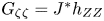 $G_{\zeta \zeta }=J^{\ast }h_{ZZ}$. Since
 $\lim _{Z\to \infty }h_{ZZ}=1$ (the dimensionless scale for curvature has been chosen to ensure that), it follows that
 $J^{\ast }$ can be read off as the
 $\zeta \to \infty$ limit of
 $G_{\zeta \zeta }$.
In the case of non-zero  $T_{\mathit {EO}}$, the situation is a little more complicated (Grassia Reference Grassia2019). If it is assumed that the values of
 $\Gamma ^{\ast }$ and
 $\chi ^{\ast }$ are known, we can solve (2.5) and obtain
 $J^{\ast }$ by the same process as in the classical system of Bretherton (Reference Bretherton1961). Formally
 $J^{\ast }$ is
 $\lim _{\zeta \to \infty }G_{\zeta \zeta }$. However, in general what we know are the values of
 $\bar {\Gamma }$ and
 $\chi '$ given by (2.2) and (2.4), not
 $\Gamma ^{\ast }$ and
 $\chi ^{\ast }$. To find the correct value of
 $J^{\ast }$, it is necessary to proceed iteratively (Grassia Reference Grassia2019), as explained in the next section.
2.3. Obtaining  $J^{\ast }$ iteratively

As mentioned above, given values of  $\bar {\Gamma }$ and
 $\chi '$, an iterative approach is required to obtain
 $J^{\ast }$, namely by guessing a value for
 $J^{\ast }$, and obtaining
 $\Gamma ^{\ast }$ and
 $\chi ^{\ast }$ via (2.6) and (2.7). Then we solve (2.5) to obtain
 $\lim _{\zeta \to \infty }G_{\zeta \zeta }$ comparing it to the guessed
 $J^{\ast }$. Generally the values differ, so the guessed value for
 $J^{\ast }$ must then be varied, and
 $\lim _{\zeta \to \infty }G_{\zeta \zeta }$ recomputed until the two values become equal (Grassia Reference Grassia2019).
It is useful to define a function  $f(J^{\ast })$ via
 \begin{equation} f(J^{\ast}) \equiv \lim_{\zeta\to\infty}G_{\zeta\zeta}(\Gamma^{\ast}(\bar{\Gamma},J^{\ast}), \chi^{\ast}(\chi',J^{\ast})) - J^{\ast} ,\end{equation}
where the notation indicates that  $\lim _{\zeta \to \infty }G_{\zeta \zeta }$ depends on
 $\Gamma ^{\ast }$ and
 $\chi ^{\ast }$ via (2.5), with
 $\Gamma ^{\ast }$ depending on both
 $\bar {\Gamma }$ and
 $J^{\ast }$ via (2.6) and with
 $\chi ^{\ast }$ depending on both
 $\chi '$ and
 $J^{\ast }$ via (2.7). The task then is to find via iteration a
 $J^{\ast }$ value such that
 \begin{equation} f(J^{\ast}) \equiv \lim_{\zeta\to\infty}G_{\zeta\zeta} - J^{\ast} = 0. \end{equation}
During the process of iteration one might be required to solve (2.5) with a selection of different  $\Gamma ^{\ast }$ and
 $\chi ^{\ast }$ values (making solution of (2.5) an important part of the overall procedure), but it is only once the correct
 $J^{\ast }$ is found that definitive values for
 $\Gamma ^{\ast }$ and
 $\chi ^{\ast }$ are determined via (2.6) and (2.7).
That (2.9) should admit a solution for  $J^{\ast }$ can be argued as follows. In the limit
 $J^{\ast }\to 0$, (2.6) gives
 $\Gamma ^{\ast }\to \infty$ so that electro-osmotic forces are absent and (2.5) reduces to the Bretherton (Reference Bretherton1961) case. This has
 $\lim _{\zeta \to \infty }G_{\zeta \zeta }$ with a known value
 $J^{\ast }_{{B}}$ where
 $J^{\ast }_{{B}}\approx 0.643$. Hence
 $\lim _{J^{\ast }\to 0}f(J^{\ast })\equiv J^{\ast }_{{B}}$, which is certainly non-zero.
The case of interest in the present work is when electro-osmotic forces are attractive (conjoining), tending to squeeze the film together, and so given any  $\Gamma ^{\ast }$ and
 $\chi ^{\ast }$ we expect films to be thinner than their classical counterparts from Bretherton (Reference Bretherton1961). Since for any given
 $\Gamma ^{\ast }$ and
 $\chi ^{\ast }$, it is
 $\lim _{\zeta \to \infty }G_{\zeta \zeta }$ that represents the thickness of the aqueous film, for attractive electro-osmotic forces, this should be smaller than
 $J^{\ast }_{{B}}$. Consequently, if we evaluate
 $f(J^{\ast })$ for
 $J^{\ast }\to J^{\ast }_{{B}}$ using (2.8), it must be the case that
 $f$ is negative.
Thus we have found that  $f>0$ for
 $J^{\ast }\to 0$, but
 $f<0$ for
 $J^{\ast }\to J^{\ast }_{{B}}$. Somewhere in the interval
 $0< J^{\ast } < J^{\ast }_{{B}}$ there must be a zero of
 $f(J^{\ast })$, assuming of course that
 $f(J^{\ast })$ is a continuous function. It is even conceivable that there might be more than one zero, i.e. a given combination of
 $\bar {\Gamma }$ and
 $\chi '$ might admit more than one film thickness, hence more than one permitted
 $J^{\ast }$, a situation that we will demonstrate later on can indeed arise.
Although we have argued for the existence of a zero of  $f(J^{\ast })$, what we will see later on is that the function
 $f(J^{\ast })$ itself is not always straightforward to evaluate. We will find that (in certain parameter regimes)
 $G_{\zeta \zeta }$ may require an exceedingly large
 $\zeta$ before it approaches anywhere near its final limiting value: this makes it challenging to compute
 $\lim _{\zeta \to \infty }G_{\zeta \zeta }$ numerically. Moreover, the value of
 $\lim _{\zeta \to \infty }G_{\zeta \zeta }$ once determined can vary abruptly with small increments in the chosen
 $J^{\ast }$. This can make it challenging to identify
 $J^{\ast }$ values at which
 $\lim _{\zeta \to \infty }G_{\zeta \zeta }$ and
 $J^{\ast }$ become equal.
In view of these challenges in identifying the  $J^{\ast }$ value that corresponds to any given choice of
 $\bar {\Gamma }$ and
 $\chi '$, for much of the study to follow we will assume that values of
 $\Gamma ^{\ast }$ and
 $\chi ^{\ast }$ are given, and will proceed to solve (2.5) without requiring foreknowledge of
 $J^{\ast }$. As was pointed out above, solving (2.5) for given
 $\Gamma ^{\ast }$ and
 $\chi ^{\ast }$ is in any case part of the overall solution procedure. Towards the end of the study, however, we will address a case in which only
 $\bar {\Gamma }$ and
 $\chi '$ are given, and
 $J^{\ast }$ must be determined as part of the problem solution.
2.4. Surface charge state of droplet surface and capillary wall
To compute with (2.5), we require a formula for  $T_{\mathit {EO}}$ and how it varies with its argument,
 $h/\epsilon _{2}$ or equivalently
 $G\,\chi ^{\ast }$. The general formula for electro-osmotic tension (Wilmott et al. Reference Wilmott, Breward and Chapman2018; Grassia Reference Grassia2019) depends on the system's surface charge on both the droplet surface and the capillary wall. In the current section therefore we consider the surface charge state, moving on to the electro-osmotic tension in the next section.
We suppose that (Wilmott et al. Reference Wilmott, Breward and Chapman2018; Grassia Reference Grassia2019) there are  $s^{\ast }$ as many charge adsorption sites per unit area on the oil droplet surface as on the capillary wall, and
 $\sigma _{c}$ and
 $\sigma _{o}$ are average charges per adsorption site on the capillary wall and oil, respectively.
In their ‘native’ state ion adsorption sites are negatively charged, and so attract positive ions (either monovalent or divalent ones) from bulk aqueous solution. Monovalent ion adsorption on any given site neutralises the negative charge there, whereas divalent ion adsorption flips charge from negative to positive. As a result, the average charge per adsorption site  $\sigma _{c}$ and
 $\sigma _{o}$ varies in principle between
 $-1$ and
 $+1$, with actual values depending on levels of ion concentrations in the aqueous phase, and also on relative amounts of monovalent and divalent ions present (Wilmott et al. Reference Wilmott, Breward and Chapman2018; Grassia Reference Grassia2019).
Values of  $\sigma _{c}$ and
 $\sigma _{o}$ are related to aqueous phase monovalent and divalent ion concentrations via Langmuir isotherm relations (Grassia Reference Grassia2019). Ion concentration levels at surfaces are a priori unknown, as they can be perturbed by electrical potentials, but in practice such perturbations are small compared with the overall ion concentrations present (Wright Reference Wright2007). The adsorption site charges
 $\sigma _{c}$ and
 $\sigma _{o}$ are hence close to the charges
 $\sigma _{c0}$ and
 $\sigma _{o0}$ that result using unperturbed bulk ion concentrations rather than perturbed ones. In what follows we use
 $\sigma _{c0}$ and
 $\sigma _{o0}$ (rather than
 $\sigma _{c}$ and
 $\sigma _{o}$) throughout.
For low ion concentrations (Wilmott et al. Reference Wilmott, Breward and Chapman2018; Grassia Reference Grassia2019) both  $\sigma _{c0}$ and
 $\sigma _{o0}$ tended to be negative (both close to
 $-1$). As overall ion concentration increased, assuming at least some level of divalent ions being present (e.g. Grassia Reference Grassia2019 considered divalent:monovalent ion concentration ratios in the range from 1 : 4 to 1 : 20), the sign of
 $\sigma _{c0}$ tended to switch to positive, whereas the sign of
 $\sigma _{o0}$ stayed negative (but
 $\sigma _{o0}$ itself reduced in magnitude). Moreover it was demonstrated that, for a given set of Langmuir isotherm parameters, it might be possible to find a set of bulk ion concentrations, that gave opposite and equal surface charges (Grassia Reference Grassia2019), i.e.
 $\sigma _{c0} + s^{\ast }\sigma _{o0} \approx 0.$ This is the specific case of interest here.
A typical value of the parameter  $s^{\ast }$ is
 $s^{\ast }\approx 10$ (i.e. 10 times more adsorption sites on oil than on the capillary wall Grassia Reference Grassia2019). A parameter set giving equal and opposite charges (amongst other possibilities) would then be
 $\sigma _{c0}=+1$,
 $\sigma _{o0}=-0.1$. We will work with these values throughout. That these choices are reasonable can be verified via the aforementioned Langmuir relations: the capillary wall must have a strong preference for divalent ion adsorption over monovalent adsorption, with the oil adsorbing significant numbers of monovalent ions but not so many divalent ones (Grassia Reference Grassia2019).
2.5. Electro-osmotic tension $T_{\mathit {EO}}$ and electro-osmotic pressure $p_{\mathit {EO}}$


In the case of interest electro-static interactions between the capillary wall and the oil–aqueous interface become attractive (conjoining) rather than repulsive (disjoining). Thus, there is a negative electro-osmotic tension  $T_{\mathit {EO}}$, or equivalently a positive electro-osmotic pressure
 $p_{\mathit {EO}}$, with
 $p_{\mathit {EO}}$ being
 $-T_{\mathit {EO}}$ here. In terms of the physics of the system, this is a change from previous studies (Wilmott et al. Reference Wilmott, Breward and Chapman2018; Grassia Reference Grassia2019) which focussed mostly on repulsive electro-osmotic interactions: the functional form for
 $p_{\mathit {EO}}$ vs
 $h/\epsilon _{2}\equiv G\,\chi ^{\ast }$ (this quantity being the ratio between the layer thickness at an arbitrary point in the transition region and the Debye screening length) turns out to be very different depending upon whether we consider the repulsive or attractive case.
In the case considered here of attractive interactions,  $p_{\mathit {EO}}$ is found to be (Grassia Reference Grassia2019)
 \begin{equation} p_{\mathit{EO}} = 2 |s^{\ast} \sigma_{c0} \sigma_{o0}| ({\cosh}(G\,\chi^{\ast}) - 1) / \sinh^{2}(G \,\chi^{\ast}).\end{equation}
In the limit  $G\,\chi ^{\ast }\gg 1$, this approximates to
 \begin{equation} p_{\mathit{EO}} \approx 4|s^{\ast} \sigma_{c0} \sigma_{o0}| \exp(-G\,\chi^{\ast}),\end{equation}
whereas, in the limit  $G\,\chi ^{\ast }\ll 1$ it approximates to
 \begin{equation} p_{\mathit{EO}} \approx |s^{\ast} \sigma_{c0} \sigma_{o0}| (1 - (G \,\chi^{\ast})^{2} / 4 ).\end{equation}
Here,  $p_{\mathit {EO}}$ has a finite limit as
 $G\,\chi ^{\ast }\to 0$, distinct from the repulsive case for which
 $T_{\mathit {EO}}$ diverges in that limit (Grassia Reference Grassia2019). Conveniently
 $|s^{\ast } \sigma _{c0} \sigma _{o0}|=1$ for our parameter set.
2.5.1. Differentiating the electro-osmotic tension
Equation (2.5) involves derivatives of electro-osmotic terms of the form  $\mathrm {d}T_{\mathit {EO}}/\mathrm {d}G$ or equivalently in our system
 $|\mathrm {d}p_{\mathit {EO}}/\mathrm {d}G|$. Therefore, to understand how electro-osmotic terms affect (2.5), it is first necessary to appreciate how
 $\mathrm {d}T_{\mathit {EO}}/\mathrm {d}G$ behaves.
In the case of interest here, although  $T_{\mathit {EO}}$ is a negative quantity, it becomes less negative as
 $G$ increases. Hence
 $\mathrm {d}T_{\mathit {EO}}/\mathrm {d}G$ (like
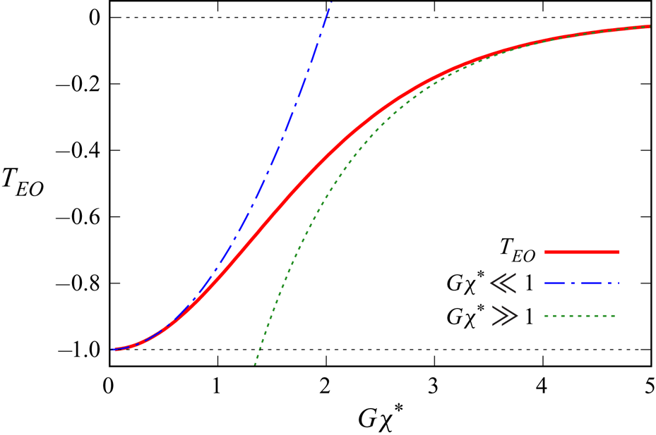
 $p_{\mathit {EO}}$ itself) is positive, as figure 2 shows. For convenience we prefer to work in terms of these positive quantities
 $\mathrm {d}T_{\mathit {EO}}/\mathrm {d}G$ and
 $p_{\mathit {EO}}$ (instead of negative quantities such as
 $\mathrm {d}p_{\mathit {EO}}/\mathrm {d}G$ and
 $T_{\mathit {EO}}$).
Electro-osmotic tension  $T_{\mathit {EO}}$ (i.e. the negative of electro-osmotic pressure
 $p_{\mathit {EO}}$) vs
 $G\,\chi ^{\ast }\equiv h/\epsilon _{2}$ (the ratio between aqueous layer thickness at an arbitrary point of the transition region and Debye screening length): see (2.10). Opposite and equal charges are assumed with
 $s^{\ast }=10$,
 $\sigma _{c0}=1$,
 $\sigma _{o0}=-0.1$. Although
 $T_{\mathit {EO}}$ is negative,
 $\mathrm {d}T_{\mathit {EO}}/\mathrm {d}G$ is positive. Asymptotic formulae for
 $G\,\chi ^{\ast }\ll 1$ and
 $G\,\chi ^{\ast }\gg 1$, respectively (2.12) and (2.11), are also plotted.
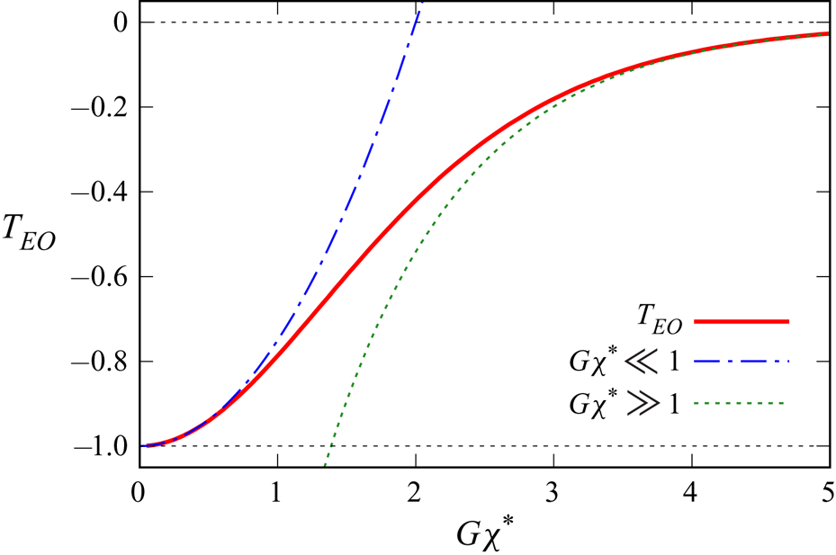
Although  $\mathrm {d}T_{\mathit {EO}}/\mathrm {d}G$ is indeed positive, (2.11) and (2.12) indicate that its value is small for both
 $G\,\chi ^{\ast }\gg 1$ and
 $G\,\chi ^{\ast }\ll 1$. Electro-osmotic effects within (2.5) are therefore weak in both limits. The result when
 $G\,\chi ^{\ast }\gg 1$ is unsurprising, since
 $p_{\mathit {EO}}$ itself decays exponentially to zero in that case. The result for
 $G\,\chi ^{\ast }\ll 1$ is slightly more surprising. Despite
 $p_{\mathit {EO}}\equiv -T_{\mathit {EO}}$ approaching a non-zero value in that limit, the variation of
 $p_{\mathit {EO}}$ about this limit is second order in
 $G \,\chi ^{\ast }$ as (2.12) shows.
The largest  $\mathrm {d}T_{\mathit {EO}}/\mathrm {d}G$ values, and hence the largest impact of electro-osmotic terms in (2.5) occurs for intermediate values of
 $G\,\chi ^{\ast }$. The maximum
 $\mathrm {d}T_{\mathit {EO}}/\mathrm {d}G$ is
 \begin{equation} \mathrm{d}T_{\mathit{EO}}/\mathrm{d}G|_{max} \approx 0.384 |s^{\ast}\sigma_{c0}\sigma_{o0}|\chi^{\ast} \quad \textrm{when } G \approx 1.316/\chi^{\ast}. \end{equation}
Note that within (2.5) we are only usually interested in values of  $G$ satisfying
 $G\ge 1$, since
 $G\equiv 1$ corresponds to the thin film region, with the transition region being thicker. Hence, there is a qualitative difference between the behaviour of
 $\mathrm {d}T_{\mathit {EO}}/\mathrm {d}G$ with respect to
 $G$ according to whether
 $\chi ^{\ast }\ge 1.316$ or
 $\chi ^{\ast }<1.316$. In the former case,
 $\mathrm {d}T_{\mathit {EO}}/\mathrm {d}G$ is a monotonically decreasing function as
 $G$ increases above
 $G=1$. In the latter case,
 $\mathrm {d}T_{\mathit {EO}}/\mathrm {d}G$ first increases then decreases as
 $G$ increases.
2.5.2. Differentiating the electro-osmotic tension in the limit $G\to 1$

Later on in our analysis, it turns out to be convenient to define a quantity  $F$ via
 \begin{equation} F \equiv \mathrm{d}T_{\mathit{EO}}/\mathrm{d}G |_{G=1}.\end{equation}
The value of  $F$ is easy to evaluate for any general
 $\chi ^{\ast }$ via differentiating (2.10). For
 $\chi ^{\ast }\gg 1$ it is clear from (2.11) that
 $F$ is small, given by
 \begin{equation} F \approx 4 |s^{\ast}\sigma_{c0}\sigma_{o0}| \chi^{\ast} \exp(-\chi^{\ast}). \end{equation}
Via (2.12), we note that for  $\chi ^{\ast }\ll 1$,
 \begin{equation} F\approx |s^{\ast}\sigma_{c0}\sigma_{o0}| \chi^{\ast\,2}/2, \end{equation}
hence is also small when  $\chi ^{\ast }\ll 1$. The maximum of
 $F$, denoted
 $F_{max}$ occurs for intermediate values of
 $\chi ^{\ast }$. It turns out that
 $F_{max}\approx 0.639 |s^{\ast }\sigma _{c0}\sigma _{o0}|$ and occurs when
 $\chi \approx 2.019$.
Note the difference between maximising  $\mathrm {d}T_{\mathit {EO}}/\mathrm {d}G$ and maximising
 $F$. If we use the symbol
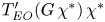
 $T'_{\mathit {EO}}$ to denote the derivative of
 $T_{\mathit {EO}}$ with respect to its argument, in the first instance we are maximising
 $T'_{\mathit {EO}}(G\,\chi ^{\ast })\,\chi ^{\ast }$ with respect to
 $G$, which is equivalent simply to finding the maximum of
 $T'_{\mathit {EO}}$. In the second instance, however, we are maximising
 $T'_{\mathit {EO}}(\chi ^{\ast })\,\chi ^{\ast }$ with respect to
 $\chi ^{\ast }$: we are not simply maximising
 $T'_{\mathit {EO}}$. Despite these subtle differences, the overall picture for
 $\mathrm {d}T_{\mathit {EO}}/\mathrm {d}G$ and for
 $F$ is similar. The former quantity is small for
 $G\,\chi ^{\ast }\ll 1$, significant for
 $G\,\chi ^{\ast }$ of the order of unity, and small again for
 $G\,\chi ^{\ast }\gg 1$. The latter quantity is small for
 $\chi ^{\ast }\ll 1$, significant for
 $\chi ^{\ast }$ of the order of unity, and small again for
 $\chi ^{\ast }\gg 1$.
2.6. Selecting parameter values for the governing equation
Back in § 2.4 we identified suitable values of the parameters  $s^{\ast }$,
 $\sigma _{c0}$ and
 $\sigma _{o0}$. However, in order to analyse the system we also need to know typical values of the parameters
 $\bar {\Gamma }$ and
 $\chi '$. Parameter value estimates have been provided by Wilmott et al. (Reference Wilmott, Breward and Chapman2018) and Grassia (Reference Grassia2019) based on literature data from various authors (Lewis Reference Lewis1937; Buckley Reference Buckley1996; Li & Xu Reference Li and Xu2008; Nelson Reference Nelson2009; Austad, Rezaei Doust & Puntervold Reference Austad, Rezaei Doust and Puntervold2010) and are reviewed below.
2.6.1. Selecting values for $\bar {\Gamma }$

A base case value for  $\bar {\Gamma }$ was selected (Grassia Reference Grassia2019) as being of the order of approximately 10, for a ‘typical’ waterflooding operation in a ‘typical’ width pore or channel (
 $R\approx 10^{-6}$ m was chosen as the channel half-width,
 $\gamma \approx 0.02$ N m
 $^{-1}$ was chosen as the interfacial tension and,following Malmberg & Maryott (Reference Malmberg and Maryott1956),
 $\varepsilon _{w}$ was taken as 56 times the permittivity of free space at the temperature of interest (Wilmott et al. Reference Wilmott, Breward and Chapman2018) close to 100
 $^{\circ }$C). Some variation in the exact value of
 $\bar {\Gamma }$ is expected owing to its dependence on channel width (see (2.2)); however, the biggest source of uncertainty is the value of
 $s_{c}^{\ast }$, the density of charge adsorption sites on the pore wall. This was estimated for kaolinite clays (using literature data of Li & Xu (Reference Li and Xu2008) as
 $10^{16}$ m
 $^{-2}$. However, the values of
 $s_{c}^{\ast }$ and hence
 $\bar {\Gamma }$ are likely to be sensitive to clay chemistry.
A detailed review of different clay chemistries is beyond the scope of the present work, but in an effort to explore sensitivity to clay chemistry, Grassia (Reference Grassia2019) considered a decrease in  $s_{c}^{\ast }$ relative to the base case by up to a factor of 10. This weakened the electro-osmotic effects and led to a 100-fold increase in
 $\bar {\Gamma }$. In the present work, by contrast, we will consider up to a 10-foldincrease in
 $s_{c}^{\ast }$, strengthening electro-osmotic effects and leading to a 100-fold decrease in
 $\bar {\Gamma }$ relative to the base case. It is for these lower
 $\bar {\Gamma }$ values that electro-osmotic effects might be able to replace capillary effects leading to a visco-electro-osmotic balance as hypothesised in the introduction. The domain of
 $\bar {\Gamma }$ of interest therefore will be
 $0.1\le \bar {\Gamma }\le 10$, but with a special focus on the lower end of the domain.
2.6.2. Selecting values for $\chi '$

We now turn to the parameter  $\chi '$. As seen in (2.4) this is the ratio between
 $(3 Ca_{{B}})^{2/3}$ and
 $\epsilon _{2}$. A base case value of
 $Ca_{{B}}$ was estimated to be (Grassia Reference Grassia2019) approximately
 $5\times 10^{-7}$ in rough order of magnitude terms. This corresponds to a flow velocity in the pores of the order of
 $10^{-5}$ m s
 $^{-1}$, a viscosity of the order of
 $10^{-3}$ Pa s, and an interfacial tension as mentioned earlier of 0.02 N m
 $^{-1}$. Since
 $Ca_{{B}}$ is directly proportional to flow velocity, we assume
 $Ca_{{B}}$ could be up to 10 times larger than the base case (for a fast waterflood) or 10 times smaller (a slower waterflood). Hence the domain of
 $Ca_{{B}}$ of interest is assumed to lie between values
 $5\times 10^{-8}$ and
 $5 \times 10^{-6}$.
Meanwhile, the value of  $\epsilon _{2}$ (which denotes here Debye length non-dimensionalised by channel half-width) is given by (Grassia Reference Grassia2019)
 \begin{equation} \epsilon_{2} = (\varepsilon_{w}k_{B}T/2 C^{+}q^{2}R^{2})^{1/2}, \end{equation}
where  $\varepsilon _{w}$ is the permittivity of the aqueous phase,
 $k_{B}$ is Boltzmann's constant,
 $T$ is absolute temperature,
 $C^{+}$ is the number density of monovalent ions,
 $q$ is electronic charge and
 $R$ is channel half-width. There is a slight change to the above expression for
 $\epsilon _{2}$ if a mixture of ions of different valencies is present (Grassia Reference Grassia2019), but this is neglected here since the change is minor and is not material to the argument to follow. According to (2.17) then, for a number density of ions of the order of
 $10^{27}$ m
 $^{-3}$ (Wilmott et al. Reference Wilmott, Breward and Chapman2018) and a channel half-width
 $10^{-6}$ m, and at the temperature mentioned earlier (100
 $^{\circ }$C or 373 K) a ‘base case’ value of
 $\epsilon _{2}$ would be approximately
 $2\times 10^{-4}$.
The value of  $\epsilon _{2}$ is, however, sensitive to ion concentration, and the value above corresponds to a high salinity flood. There have been reports in the literature (Yildiz & Morrow Reference Yildiz and Morrow1996; McGuire et al. Reference McGuire, Chatham, Paskvan, Sommer and Carini2005; Lager et al. Reference Lager, Webb, Black, Singleton and Sorbie2008; Ligthelm et al. Reference Ligthelm, Gronsveld, Hofman, Brussee, Marcelis and van der Linde2009; Austad et al. Reference Austad, Rezaei Doust and Puntervold2010; Rezaei Doust et al. Reference Rezaei Doust, Puntervold and Austad2011) of performing waterfloods with water that is far less saline than seawater, with ion number densities around
 $10^{25}$ m
 $^{-3}$ being typical. This gives a 10-fold increase in
 $\epsilon _{2}$ relative to the aforementioned base case, up to
 $2\times 10^{-3}$ instead of
 $2\times 10^{-4}$.
Given these domains for  $Ca_{{B}}$ and
 $\epsilon _{2}$, we estimate
 $\chi '$ given by (2.4) could vary approximately between 0.02 and 5, with the lower end value corresponding to a low speed and low salinity waterflood, and the upper end being for high speed and high salinity.
This completes our estimates of the key parameters  $\bar {\Gamma }$ and
 $\chi '$. In what follows, however, often we prefer to work with (2.5), which involves parameters
 $\Gamma ^{\ast }$ and
 $\chi ^{\ast }$. Estimates for these parameters are discussed next.
2.6.3. Selecting values for $\Gamma ^{\ast }$ and $\chi ^{\ast }$


The parameters  $\Gamma ^{\ast }$ and
 $\chi ^{\ast }$ are related to
 $\bar {\Gamma }$ and
 $\chi '$ via (2.6) and (2.7), but the parameter
 $J^{\ast }$ in those equations is a priori unknown, and must be found to satisfy (2.9). As a result the domain of interest for parameters
 $\bar {\Gamma }$ and
 $\chi ^{\ast }$ is a priori unknown.
For large  $\bar {\Gamma }$ and/or large
 $\chi '$ (Grassia Reference Grassia2019),
 $J^{\ast }$ is found to approach the known value
 $J^{\ast }_{{B}}\approx 0.643$. Clearly,
 $J^{\ast }_{{B}}$ is an order-unity value, and on the basis of this we will, in the first instance, explore
 $\Gamma ^{\ast }$ values over the same domain as
 $\bar {\Gamma }$ (values down to 0.1) and
 $\chi ^{\ast }$ values over the same domain as
 $\chi '$ (between 0.02 and 5). Later, however, we will discover that for smaller
 $\bar {\Gamma }$ and/or
 $\chi '$ values, the value of
 $J^{\ast }$ can be significantly smaller than
 $J^{\ast }_{{B}}$. Via (2.6) and (2.7) the system thereby selects a
 $\Gamma ^{\ast }$ that is rather larger than
 $\bar {\Gamma }$ and likewise selects a
 $\chi ^{\ast }$ that is rather smaller than
 $\chi '$. The consequences of this in terms of how it affects the shape of the droplet will be described towards the end of the paper.
2.7. Linearisation of the governing equation
We said earlier that (2.5) must be integrated numerically to obtain  $\lim _{\zeta \to \infty } G_{\zeta \zeta }$, which represents the thickness of the aqueous film for a given
 $\Gamma ^{\ast }$ and
 $\chi ^{\ast }$.
To start the numerical integration, we need to know values of  $G$,
 $G_{\zeta }$ and
 $G_{\zeta \zeta }$ at one particular
 $\zeta$ value. We follow an established procedure for this (Bretherton Reference Bretherton1961; Wilmott et al. Reference Wilmott, Breward and Chapman2018; Grassia Reference Grassia2019). Specifically, we choose an arbitrary point at which
 $G=1+\varepsilon$ where
 $\varepsilon$ is any small value, such that
 $\varepsilon \ll 1$. As in Grassia (Reference Grassia2019), we choose
 $\varepsilon =10^{-5}$. Without loss of generality, this point is taken to correspond to
 $\zeta =0$. We then linearise the governing equation for small values of
 $G-1$, obtaining a solution
 $G\approx 1 + \varepsilon \exp (\Lambda \zeta )$ such that
 $\Lambda$ satisfies
 $\Lambda ^{3} = 1 - \Lambda F/\Gamma ^{\ast }$, where
 $F$ was defined in (2.14). Note that, if
 $F$ is small or
 $\Gamma ^{\ast }$ is large, then
 $\Lambda$ is always close to unity. However, if
 $\Gamma ^{\ast }$ is much smaller than
 $F$ (the maximum possible value of
 $F$ being
 $F_{max}$ as per § 2.5.2), then
 $\Lambda$ approaches
 $\Gamma ^{\ast }/F$ which would then be rather smaller than unity.
Although exponential growth of  $G$ with increasing
 $\zeta$ is predicted here, the growth could be quite short-lived depending on the value of
 $\Lambda$, since nonlinear effects eventually become significant. Even if the exponential growth is short-lived, however, at least in some neighbourhood of
 $\zeta =0$, we have
 $G_{\zeta }\approx \Lambda (G-1)$ and
 $G_{\zeta \zeta }\approx \Lambda ^{2}(G-1)$. This information is sufficient to start the numerical integration of (2.5), which then proceeds via the method described in the next section.
2.8. Numerical method
As was the case in Grassia (Reference Grassia2019), the numerical method used to solve (2.5) was the Runge–Kutta method (Press et al. Reference Press, Teukolsky, Vetterling and Flannery1992). We used a Runge–Kutta step size of  ${\rm \Delta} \zeta =0.02$. The integration needs to be continued until such a point that
 $G_{\zeta \zeta }$ has converged to a final value, which we denote
 $G_{\zeta \zeta ,\infty }$ (shorthand notation for
 $\lim _{\zeta \to \infty } G_{\zeta \zeta }$).
Owing to us exploring a different parameter regime from the one that was considered in Grassia (Reference Grassia2019) (i.e. attractive electro-osmotic interactions and comparatively small  $\bar {\Gamma }$ are considered here) we found that sometimes we needed to reach extremely large
 $\zeta$ values to approach a final converged
 $G_{\zeta \zeta }$ value. Some of the numerical data we show later on for instance only attain convergence for
 $\zeta \ge 1000$. In the context of a droplet in a capillary channel, this corresponds to an exceedingly long transition region.
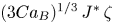
Recall from § 2.2.1 that the longitudinal coordinate  $Z$ is
 $(3 Ca_{{B}})^{1/3}\, J^{\ast } \, \zeta$ where
 $Ca_{{B}}$ denotes capillary number, and
 $J^{\ast }$ denotes dimensionless film thickness. If we assume that
 $J^{\ast }$ is order unity, and recall that the smallest
 $Ca_{{B}}$ we consider is approximately
 $5\times 10^{-8}$, then with
 $\zeta \approx 1000$, the transition region is already approximately five times the half-width of the channel in which the droplet is contained. Of course the droplet may still be somewhat longer than that, since it is possible to have a very elongated droplet migrating through a capillary pore. Nonetheless, it is clear that the classical asymptotic picture (Bretherton Reference Bretherton1961) of a flat aqueous film covering most of the length of the droplet, with a compact transition region separating the flat film from curved capillary static ends has already broken down in this limit. Any parameter sets that require exceedingly large
 $\zeta$ in order for
 $G_{\zeta \zeta }$ to converge, should therefore be interpreted with caution.
Note that the argument above requiring us to keep  $\zeta$ less than approximately 1000, relies on assuming
 $J^{\ast }$ being order unity. If it turns out that
 $J^{\ast }$ is significantly smaller than unity (owing to attractive electro-osmotic interactions reducing film thickness), more flexibility would be permitted in the domain for
 $\zeta$, which could be expanded by a factor
 $(J^{\ast })^{-1}$.
Clearly therefore establishing the value of  $J^{\ast }$ is important, and the other numerical procedure that we must implement is to find the a priori unknown
 $J^{\ast }$ value that satisfies
 $f(J^{\ast })=0$ as per (2.9). Here a bisection method was used, remembering from § 2.3 that there should be a zero of the function
 $f$ over the interval
 $0\le J^{\ast }\le J^{\ast }_{{B}}$. The reason we used a bisection method rather than some other method (e.g. Newton–Raphson (Press et al. Reference Press, Teukolsky, Vetterling and Flannery1992) with a numerical estimate of
 $\mathrm {d}f/\mathrm {d}J^{\ast }$) is that in certain parameter regimes we will see that
 $f$ turns out to be an ill-behaved function with multiple maxima and minima, and with abrupt changes with very large derivatives in places. This can make it difficult to attain convergence with the Newton–Raphson method.
3. Analysis of the governing equations
We have now completed our presentation of the governing equations, the parameter values for which they are to be solved and the numerical solution technique. Before proceeding to consider numerical results themselves (within § 4), we will first analyse a number of limiting cases of the governing equations. These limiting cases will provide a conceptual framework to understand better the behaviour of the numerical results.
This section is laid out as follows. Section 3.1 considers a regime in which viscous and electro-osmotic effects can balance, whilst § 3.2 considers an alternative balance, namely a capillary, electro-osmotic one. Sections 3.3 and 3.4 estimate the a priori unknown parameter  $J^{\ast }$ that satisfies (2.9).
For the benefit of readers who wish to skip the details and proceed direct to § 4, we highlight the following key results. Section 3.1 predicts shapes of the transition region  $G$ vs
 $\zeta$ via two key equations (3.2) and (3.3). These shapes can be such that
 $G$ grows surprisingly slowly with
 $\zeta$ for quite some distance (see (3.5) and (3.6)). However,
 $G$ eventually is predicted to diverge at finite
 $\zeta$, an artefact of neglecting capillarity. Section 3.2 predicts oscillatory solutions for
 $G$ vs
 $\zeta$ (see (3.8)), such solutions being plausible, even when capillarity is inherently weak, provided oscillations are short wavelength. A key equation is (3.9), which indicates that during an oscillation cycle
 $G_{\zeta \zeta }$ tracks the value of the electro-osmotic pressure
 $p_{\mathit {EO}}(G\,\chi ^{\ast })$, but with intermittent changes possible from one oscillation cycle to the next. Section 3.3 derives a useful estimate of film thickness (3.12), in the case of a film that is sufficiently thin that charge screening effects are irrelevant (so that the parameter
 $\chi '\to 0$). Section 3.4 derives an ad hoc estimate for film thickness over a wide range of
 $\chi '$ (see (3.14)).
3.1. Visco-electro-osmotic limit
In the introduction we suggested that it might be possible for the system to approach a visco-electro-osmotic limit for which capillary terms are neglected over at least part of the domain. Using the analysis of the foregoing sections we can now estimate conditions under which such a state might or might not arise, as explained below.
3.1.1. Governing equations for visco-electro-osmotic model
It is clear that if  $\Gamma ^{\ast }\gg 1$, electro-osmotic terms in (2.5) are never important, and hence a visco-electro-osmotic balance requires having
 $\Gamma ^{\ast }$ less than or equal to order unity. Secondly, it is clear from (2.11) that if
 $G\,\chi ^{\ast }\gg 1$ then electro-osmotic terms decay exponentially, so a visco-electro-osmotic balance requires
 $G\,\chi ^{\ast }$ of order unity or less. Since we expect
 $G \ge 1$ always, it follows that
 $\chi ^{\ast }$ must itself be at most order unity for an electro-osmotic balance to apply. The smaller the value of
 $\chi ^{\ast }$ therefore, the larger the possible domain for
 $G$ over which such a balance could apply.
Suppose we introduce a new coordinate variable  $\zeta '$ via
 $\zeta ' \equiv \Gamma ^{\ast } \zeta / F$, where
 $F$ is defined by (2.14). Written in terms of
 $\zeta '$, (2.5) becomes
 \begin{equation} \left(\frac{\Gamma^{\ast}}{F}\right)^{3} G_{\zeta'\zeta'\zeta'} = \frac{G-1}{G^{3}} - \frac{T'_{\mathit{EO}}(G \,\chi^{\ast})}{T'_{\mathit{EO}}(\chi^{\ast})} G_{\zeta'}.\end{equation}
We are interested here in situations with  $\Gamma ^{\ast }\ll 1$. Provided
 $\Gamma ^{\ast }\ll F$, the capillary term on the left-hand side of (3.1) can be neglected, and we obtain
 \begin{equation} \frac{\mathrm{d}G}{\mathrm{d}\zeta'} \approx \frac{{G-1}}{G^{3}} \frac{T'_{\mathit{EO}}(\chi^{\ast})}{T'_{\mathit{EO}}(G\chi^{\ast})} \equiv \frac{{G-1}}{G^{3}} \frac{F}{\mathrm{d}T_{\mathit{EO}}/\mathrm{d}G}. \end{equation}
For  $\Gamma ^{\ast } \ll F$ to apply, (2.15) and (2.16) imply that
 $\chi ^{\ast }$ must satisfy both
 $\chi ^{\ast }\le O(1)$ and
 $\Gamma ^{\ast }/|s^{\ast }\sigma _{c0}\sigma _{o0}|\ll \chi ^{\ast \,2}$ (with
 $|s^{\ast }\sigma _{c0}\sigma _{o0}|=1$ here). Thus the visco-electro-osmotic limit applies for small
 $\Gamma ^{\ast }$ and small to moderate
 $\chi ^{\ast }$.
Equation (3.2) can also be converted back to the original set of variables giving
 \begin{equation} \frac{\mathrm{d}G}{\mathrm{d}\zeta} \approx \Gamma^{\ast}\frac{{G-1}}{G^{3}} \frac{1}{\chi^{\ast} T'_{\mathit{EO}}(G\,\chi^{\ast})} \equiv \Gamma^{\ast}\frac{{G-1}}{G^{3}} \frac{1}{\mathrm{d}T_{\mathit{EO}}/\mathrm{d}G}.\end{equation}
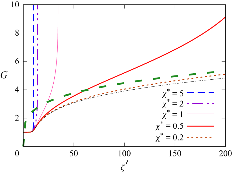
Via quadrature, solutions of (3.2) or (3.3) can be obtained in implicit form ( $\zeta '$ or
 $\zeta$ as functions of
 $G$). Features of these solutions are discussed in what follows.
3.1.2. Analytical approximations to the visco-electro-osmotic model
In the limit of  $\chi ^{\ast }$ rather smaller than unity, there is a range of
 $G$ values (those values satisfying
 $G\,\chi ^{\ast }\ll 1$), such that
 $F/(\mathrm {d}T_{\mathit {EO}}/\mathrm {d}G)\approx G^{-1}$, as follows from (2.12) and (2.16). Equation (3.2) then simplifies to
 \begin{equation} \mathrm{d}G/\mathrm{d}\zeta' = (G - 1) / G^{4}. \end{equation}
This has exponential growth for  $G$ when
 $G-1$ is small, but the behaviour soon departs from exponential. In fact, on the basis of (3.4), it is possible to show that
 $G$ vs
 $\zeta '$ has an inflection point at
 $G=\frac {4}{3}$. An exponential of course has no such inflection.
The solution of (3.4) is
 \begin{align} \zeta' = G^{4}/4 + G^{3}/3 + G^{2}/2+ G+ \log((G-1)/\varepsilon) -\varepsilon^{4}/4 -4 \varepsilon^{3}/3 -3 \varepsilon^{2} -4 \varepsilon- 25/12. \end{align}
Moreover, if  $G\gg 1$ (but still assuming
 $G\,\chi ^{\ast }\ll 1$), this simplifies to
 \begin{equation} G \approx (4 \zeta')^{1/4}. \end{equation}
Note that this implies that the growth of  $G$ becomes increasingly slow as
 $\zeta '$ increases.
The value of  $G$ can only start to increase very significantly (overcoming the aforementioned increasingly slow growth) when
 $G\,\chi ^{\ast }$ exceeds order unity, at which point (3.6) breaks down, since
 $F/(\mathrm {d}T_{\mathit {EO}}/\mathrm {d}G)$ ceases to be approximated by
 $G^{-1}$. If we use (3.6) to provide a rough estimate of when
 $G\,\chi ^{\ast }$ might first attain values of order unity, and hence
 $G$ might attain values of order
 $1/\chi ^{\ast }$, we determine
 $\zeta ' \sim O((\chi ^{\ast })^{-4})$. This result can also be expressed in terms of
 $\zeta$ giving
 $\zeta \equiv F \zeta '/\Gamma ^{\ast } \sim O((\chi ^{\ast })^{-2}\, (\Gamma ^{\ast })^{-1})$ where
 $F$ has been estimated via (2.16). In the limit of small
 $\chi ^{\ast }$, this predicts extremely large
 $\zeta '$ and/or
 $\zeta$ values for
 $G\,\chi ^{\ast }$ to exceed unity. Growth in
 $G$ with respect to the coordinate
 $\zeta '$ and/or
 $\zeta$ is therefore very slow in this small
 $\chi ^{\ast }$ limit. The asymptotic picture whereby the aqueous thin film joins up with a capillary static region across a compact transition region might be no longer valid in that case.
3.1.3. Divergence of the visco-electro-osmotic model
So far discussion of the visco-electro-osmotic model has considered values of  $G\,\chi ^{\ast }$ up to order unity. It is interesting to examine how the model breaks down once
 $G\,\chi ^{\ast }$ becomes significantly larger than unity, so that
 $\mathrm {d}T_{\mathit {EO}}/\mathrm {d}G$ decays exponentially via (2.11). According to (3.2),
 $\mathrm {d}G/\mathrm {d}\zeta '$ then becomes so large that
 $G$ diverges to infinity at finite
 $\zeta '$. The divergence happens so rapidly after
 $G\,\chi ^{\ast }$ exceeds order unity, that the estimates
 $\zeta ' \sim O((\chi ^{\ast })^{-4})$ and
 $\zeta \sim O((\chi ^{\ast })^{-2}\, (\Gamma ^{\ast })^{-1})$ given in § 3.1.2 can be used to estimate not only where
 $G\,\chi ^{\ast }$ attains order unity, but also where the divergence occurs. Of course, before
 $G$ diverges, (3.2) has ceased to be a good approximation to (2.5). The electro-osmotic term is now so weak, it is no longer tenable to retain electro-osmotic effects but neglect capillary ones. Another regime in which capillary effects make an essential contribution to the shape of the profile is discussed next.
3.2. Oscillatory behaviour for $G$ vs $\zeta$


Equation (3.1) was used to justify the neglect of capillary terms when  $\Gamma ^{\ast }\ll F$ or equivalently, for small to moderate
 $\chi ^{\ast }$ values, when
 $\Gamma ^{\ast }/| s^{\ast } \sigma _{c0} \sigma _{o0}|\ll \chi ^{\ast \,2}$. This led to
 $G$ evolving over very long length scales, e.g.
 $\zeta '$ values up to
 $O((\chi ^{\ast })^{-4})$ or
 $\zeta$ values up to
 $O((\chi ^{\ast })^{-2}(\Gamma ^{\ast })^{-1})$.
The capillary term in (3.1) can, however, retain importance if  $G$ exhibits oscillations on much shorter length scales than those mentioned above. Conditions under which this might happen are explored here.
3.2.1. Capillary, electro-osmotic balance
Suppose we define  $\hat \zeta = (\chi ^{\ast }/\Gamma ^{\ast })^{1/2}\,\zeta$ and
 $\hat G=G\,\chi ^{\ast }$. Equation (2.5) now becomes
 \begin{equation} \hat G_{{\hat\zeta}{\hat\zeta}{\hat\zeta}} = \left({\Gamma^{\ast}\,\chi^{\ast}}\right)^{3/2} \frac{\hat G-\chi^{\ast}}{ \hat G^{3}} - T'_{\mathit{EO}} (\hat G) \hat G_{\hat\zeta}. \end{equation}
If the product  $\Gamma ^{\ast }\,\chi ^{\ast } \equiv \bar \Gamma \,\chi '$ is small, the viscous term is negligible, and a capillary, electro-osmotic balance results.
Converting back to the original variable set, gives
 \begin{equation} G_{\zeta\zeta\zeta}\approx-\frac{\mathrm{d}T_{\mathit{EO}}/\mathrm{d}G}{\Gamma^{\ast}} \, G_{\zeta}. \end{equation}
This corresponds to an augmented Young–Laplace equation (Teletzke et al. Reference Teletzke, Davis and Scriven1988), but differs from augmented Young–Laplace systems previously discussed by Grassia (Reference Grassia2019).
That earlier work (Grassia Reference Grassia2019) focussed primarily on a case with repulsive charges such that  $\mathrm {d}T_{\mathit {EO}}/\mathrm {d}G$ was large and negative in the small
 $\chi ^{\ast }$ limit. That gave monotonic growth of
 $G$ vs
 $\zeta$, whereas here (with
 $\mathrm {d}T_{\mathit {EO}}/\mathrm {d}G >0$ as per figure 2) oscillatory behaviour is anticipated. As was mentioned in § 1.1, oscillatory behaviour is seen in the classical system (without electro-osmotic effects), but only at the back of a droplet (Bretherton Reference Bretherton1961; Wilmott et al. Reference Wilmott, Breward and Chapman2018), not at the front, as we are currently considering. It is known also that adding repulsive electro-osmotic effects to the back of the droplet actually removes the oscillatory behaviour (Wilmott et al. Reference Wilmott, Breward and Chapman2018). Here, on the other hand, we are talking about adding attractive electro-osmotic effects to the front of the droplet, and this potentially can introduce oscillations even though there were none originally.
Equation (3.8) is the equation of an oscillator, but since  $\mathrm {d}T_{\mathit {EO}}/\mathrm {d}G$ is variable (varying in the fashion described in § 2.5.1), it is a nonlinear oscillator. The wavelength of the oscillations will therefore vary with
 $G$, and tends to be smaller in a parameter range where
 $\mathrm {d}T_{\mathit {EO}}/\mathrm {d}G$ is larger: as mentioned in § 2.5.1,
 $\mathrm {d}T_{\mathit {EO}}/\mathrm {d}G$ is maximal when
 $G$ is order
 $1/\chi ^{\ast }$, i.e.
 $\hat G$ is order unity. It is clear, however, from (3.8) that the smaller the value of
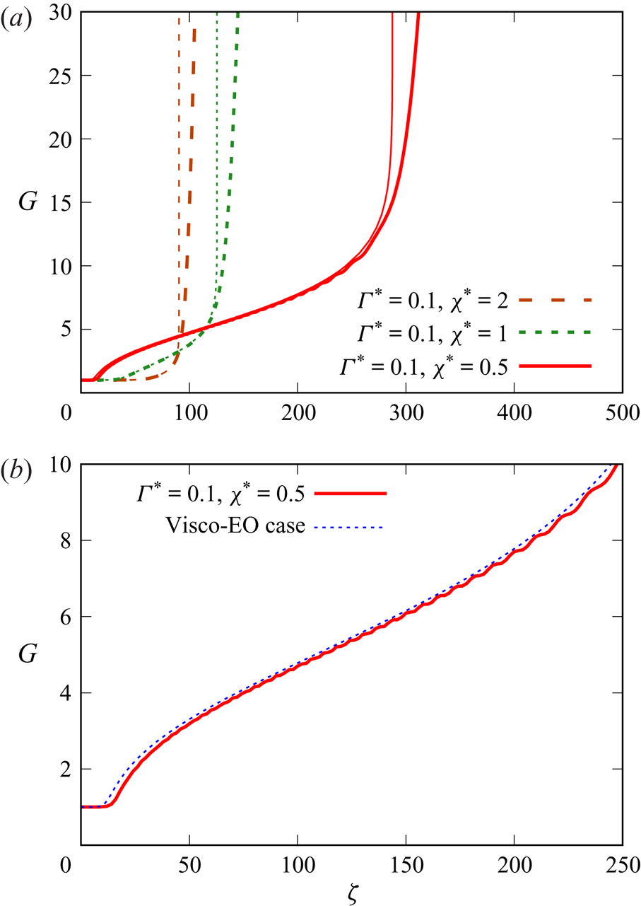
 $\Gamma ^{\ast }$, the smaller the wavelength of the oscillations tends to be. Short wavelength oscillations help to ensure that capillary terms (which correspond to the highest-order spatial derivatives in the system) can become non-negligible.
3.2.2. Transition from oscillatory to non-oscillatory behaviour
Although (3.8) does describe an oscillator, we know that if ever  $G\,\chi ^{\ast }$ manages to grow significantly larger than unity, electro-osmotic effects are screened in an exponential fashion, the value of
 $\mathrm {d}T_{\mathit {EO}}/\mathrm {d}G$ decays, and the oscillations must increase in wavelength and eventually stop. Either a capillary static state must then be attained, or more generally, a classical capillary, viscous balance (Bretherton Reference Bretherton1961) might then ensue. Either way, in such a system, at sufficiently large
 $\zeta$, the value of
 $G_{\zeta \zeta }$ should approach a well-defined limit
 $G_{\zeta \zeta ,\infty }$. Using this fact it is possible to describe in more detail how the system behaves as it transitions from an oscillatory to a non-oscillatory state.
It is possible to write (2.5) in the form
 \begin{equation} G_{\zeta\zeta} - \frac{1}{\Gamma^{\ast}} p_{\mathit{EO}}(G\,\chi^{\ast}) =G_{\zeta\zeta,\infty} - \int_{\zeta}^{\infty}\frac{{G-1}}{G^{3}} \,\mathrm{d}\zeta. \end{equation}
Like (3.8), this describes a nonlinear oscillator, and moreover provided  $\Gamma ^{\ast }$ is small (as we suppose here), oscillations have short wavelength as mentioned earlier. Notice, however, that (3.9) has a right-hand side that evolves, being an increasing function of
 $\zeta$, albeit with the evolution of that right-hand side being slow compared to the typical wavelength of each oscillation. This then is a multiple scales problem, and we anticipate (Kuzmak Reference Kuzmak1959) that the value of
 $G$ averaged over each oscillation cycle undergoes some slow secular change with coordinate
 $\zeta$.
We assume also that  $\chi ^{\ast }$ is small,
 $\chi ^{\ast }\ll 1$, and consider a situation whereby during each oscillation
 $G$ varies between a value of order unity, and a much larger value of order
 $O(1/\chi ^{\ast })$, any larger amplitude oscillation being impossible due to
 $p_{\mathit {EO}}$ decaying at large
 $G\,\chi ^{\ast }$. Any part of the oscillation cycle during which
 $G$ is
 $O(1/\chi ^{\ast })$ should make a negligible contribution to the integrated term on the right-hand side of (3.9). The only non-negligible contributions to that integrated term arise intermittently, i.e. once per oscillation cycle, around the point at which
 $G$ has its
 $O(1)$ minimum. This then is what drives secular change. As the secular change in
 $G$ accumulates, eventually the oscillations cease, for the reason pointed out above, i.e.
 $p_{\mathit {EO}}$ decays.
Note also that at the minimum of each oscillation cycle for  $G$, the value of
 $p_{\mathit {EO}}$ is a maximum. According to (2.12), this maximal
 $p_{\mathit {EO}}$ should be roughly
 $|s^{\ast }\sigma _{c0}\sigma _{o0}|$, and should, moreover, barely change from one oscillation cycle to the next given that (2.12) exhibits only second-order variation when
 $G\,\chi ^{\ast }\ll 1$. It follows also that
 $G_{\zeta \zeta }$ on the left-hand side of (3.9) is a maximum when
 $G$ is a minimum. Moreover, since any secular change in the right-hand side of (3.9) happens around the point in the cycle where
 $G$ is minimal, we should see secular changes in the maximum
 $G_{\zeta \zeta }$ value that is attained from one oscillation cycle to the next. Each oscillation should thereby give an increment to
 $G_{\zeta \zeta }$ and eventually, for
 $\zeta$ sufficiently large,
 $G_{\zeta \zeta }$ should attain some final value
 $G_{\zeta \zeta ,\infty }$.
An expression for  $G_{\zeta \zeta ,\infty }$ can be obtained by evaluating (3.9) in the limit
 $\zeta \to -\infty$, which corresponds to
 $G\to 1$ and
 $G_{\zeta \zeta }\to 0$. Hence (using also (2.6))
 \begin{equation} G_{\zeta\zeta,\infty} = \int_{-\infty}^{\infty} \frac{{G-1}}{G^{3}} \,\mathrm{d}\zeta - \frac{p_{\mathit{EO}}(\chi^{\ast})}{\Gamma^{\ast}} = \int_{-\infty}^{\infty} \frac{{G-1}}{G^{3}} \,\mathrm{d}\zeta - \frac{J^{\ast} p_{\mathit{EO}}(\chi^{\ast})}{\bar{\Gamma}}. \end{equation}
As noted above, (2.12) shows that  $p_{\mathit {EO}}(\chi ^{\ast })$ for small
 $\chi ^{\ast }$ should approach
 $|s^{\ast } \sigma _{c0}\sigma _{o0}|$, with only second-order variation with
 $\chi ^{\ast }$. Under these circumstances, variation in
 $G_{\zeta \zeta ,\infty }$ as a function of
 $\chi ^{\ast }$ therefore depends on variation in the integrated term within (3.10). Each oscillation in
 $G$ should contribute to this integrated term, and hence the more oscillatory is the function
 $G$, the larger is the value of
 $G_{\zeta \zeta ,\infty }$ that we expect.
3.3. Estimating $J^{\ast }$ in the small $\bar {\Gamma }$ and $\chi '$ limit


In the previous sections we considered cases in which  $\Gamma ^{\ast }$ and
 $\chi ^{\ast }$ were given, and (2.5) could be solved directly. The value of
 $J^{\ast }$ (the dimensionless film thickness) could then be read off as
 $G_{\zeta \zeta ,\infty }\equiv \lim _{\zeta \to \infty } G_{\zeta \zeta }$. In general, however, we are not given values of
 $\Gamma ^{\ast }$ and
 $\chi ^{\ast }$ up front, but instead values of
 $\bar {\Gamma }$ and
 $\chi '$. Equations (2.6) and (2.7) can only be used to obtain
 $\Gamma ^{\ast }$ and
 $\chi ^{\ast }$ once the a priori unknown parameter
 $J^{\ast }$ is determined.
As has already been mentioned (see §§ 2.3 and 2.6.3), in the classical system of Bretherton (Reference Bretherton1961) (without electro-osmotic terms), corresponding to limits  $\bar {\Gamma }\to \infty$ or
 $\chi '\to \infty$, the value of
 $J^{\ast }$ is known to be
 $J^{\ast }_{{B}}\approx 0.643$. Here, however, we have a system with attractive electro-osmotic interactions which could be rather strong (
 $\bar {\Gamma }$ less than order unity) and need not be screened out (
 $\chi '$ of order unity or less). Film thickness
 $J^{\ast }$ might then be rather less than
 $J^{\ast }_{{B}}$. Ordinarily
 $J^{\ast }$ is found by solving (2.9) but as § 2.3 explained, this can be a laborious iterative process. A direct estimate for
 $J^{\ast }$ in cases with
 $J^{\ast }\ll 1$, bypassing a laborious solution for (2.9), would be useful. A way to do this is discussed below.
3.3.1. Methodology for estimating $J^{\ast }$ for small $\chi '$


We proceed as follows. Small  $\chi '$ (and hence small
 $\chi ^{\ast }$ via (2.7) tends to imply small second-order variation with respect to
 $G$ of the electro-osmotic pressure via (2.12), even though
 $p_{\mathit {EO}}$ itself might be non-zero. As a first approximation we integrate (2.5) ignoring electro-osmotic pressure gradient terms over a subdomain from
 $G=1$ to a
 $G$ value satisfying
 $1\ll G \ll 1/\chi ^{\ast }$. Since the final
 $G$ value in the subdomain of interest satisfies
 $G\gg 1$, and we solve a classical capillary, viscous problem there (Bretherton Reference Bretherton1961) it follows that
 $G_{\zeta \zeta }$ attains a value approximately
 $J^{\ast }_{{B}}\approx 0.643$.
Our next task is to continue integrating (2.5) over a new subdomain from a value  $1\ll G\ll 1/\chi ^{\ast }$ to a value
 $G\gg 1/\chi ^{\ast }$ at which point
 $G_{\zeta \zeta }$ has changed from
 $J^{\ast }_{{B}}$ to some final limiting value
 $G_{\zeta \zeta ,\infty }$. On the grounds that
 $G\gg 1$ in this new subdomain, we assume that the viscous term in (2.5) can be neglected, or equivalently the integral term in (3.9) can be neglected. Gradients of electro-osmotic terms, however, are relevant when
 $G\,\chi ^{\ast }$ is order unity, with the change in
 $G_{\zeta \zeta }$ across the subdomain reflecting the change in the electro-osmotic pressure, which from (2.11) and (2.12) is
 $|s^{\ast } \sigma _{c0}\sigma _{o0}|$ between the limits
 $G\,\chi ^{\ast }\ll 1$ and
 $G\,\chi ^{\ast }\gg 1$. Hence (2.5) gives
 \begin{equation} {G_{\zeta\zeta,\infty} \approx J^{\ast}_{{B}} - {|s^{\ast} \sigma_{c0}\sigma_{o0}|}{/\Gamma^{\ast}} \equiv J^{\ast}_{{B}} -J^{\ast}{|s^{\ast} \sigma_{c0}\sigma_{o0}|}{/\bar{\Gamma}}}\end{equation}
where (2.6) has also been used. The above result can also be derived directly from (3.10) recognising that the integral term in that equation is now contributed almost entirely from the first subdomain, and evaluates to  $J^{\ast }_{{B}}$ since a classical capillary, viscous balance applies in that subdomain. Observe that
 $G_{\zeta \zeta ,\infty }\le J^{\ast }_{{B}}$. The implication is that
 $G_{\zeta \zeta }$ is no longer a monotonically increasing function of
 $\zeta$, by contrast with what happens in the classical system of Bretherton (Reference Bretherton1961). Rather
 $G_{\zeta \zeta }$ is an increasing function of
 $\zeta$ on the first subdomain, but a decreasing function on the second subdomain.
We now determine  $J^{\ast }$ by imposing the condition within (3.11) that
 $G_{\zeta \zeta ,\infty }=J^{\ast }$ thereby enforcing (2.9). Rearranging (3.11) leads to
 \begin{equation} {J^{\ast}|_{\chi'\to 0} \approx J^{\ast}_{{B}} \, {\bar{\Gamma}}{/(\bar{\Gamma} + |s^{\ast}\sigma_{c0}\sigma_{o0}|)}.} \end{equation}
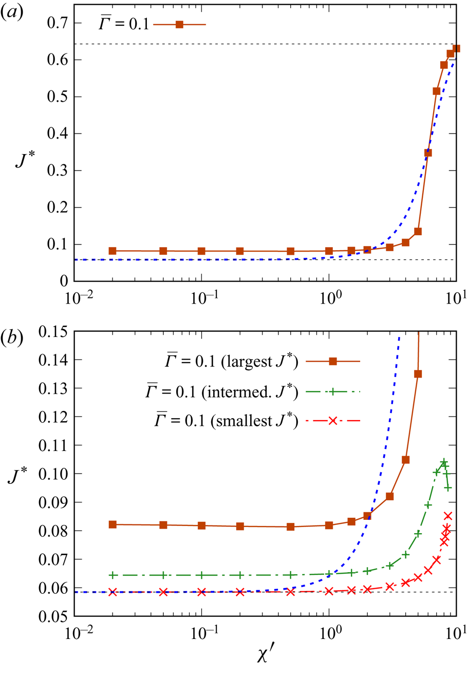
Here, recall that  $|s^{\ast }\sigma _{c0}\sigma _{o0}|=1$ (see § 2.4) and hence, if
 $\bar {\Gamma }\ll 1$, then
 $J^{\ast }\ll J^{\ast }_{{B}}$.
Given this (very small)  $J^{\ast }$ value, (2.6) now implies a value for
 $\Gamma ^{\ast }$
 \begin{equation} \Gamma^{\ast} \approx (\bar{\Gamma} + | s^{\ast}\sigma_{c0}\sigma_{o0}|) / J^{\ast}_{{B}}, \end{equation}
which is never exceedingly small, even if  $\bar {\Gamma }\ll 1$. Whereas an exceedingly small
 $\Gamma ^{\ast }$ might have caused
 $G$ itself to become oscillatory with
 $\zeta$ with very short wavelength oscillations, here, however, with
 $\Gamma ^{\ast }$ being somewhat larger, oscillation wavelengths in
 $\zeta$ grow (based on § 3.2.1, they must scale as order
 $(\Gamma ^{\ast }/\chi ^{\ast })^{1/2}$ or equivalently
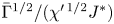 $\bar \Gamma ^{1/2}/(\chi ^{\prime \,1/2}J^{\ast })$), and the role of the electro-osmotic term seems to be to introduce non-monotonicity in
 $G_{\zeta \zeta }$, but not necessarily in
 $G$ itself. Another way to reach the same conclusion is to convert back from the coordinate
 $\zeta$ to the original coordinate
 $Z$ (see § 2.2.1). Since a factor
 $J^{\ast }$ appears in the conversion, we conclude that the length scale in
 $Z$ for secular growth in
 $G$ is compressed as
 $J^{\ast }$ decreases so that the film becomes thinner, whereas the length scale for oscillations is relatively insensitive to thickness when expressed in terms of
 $Z$ as opposed to
 $\zeta$ (as mentioned above, it scales like
 $(J^{\ast })^{-1}$ when expressed in terms of
 $\zeta$). Thus the response for
 $G$ shifts away from oscillation towards secular growth.
Equations (3.12) and (3.13) are only approximations, and in reality  $J^{\ast }$ can only be found for any given
 $\bar {\Gamma }$ and
 $\chi '$ by solving (2.9) iteratively. Nonetheless (3.12) does give an indication of where one might start the iteration. The implication for (2.5) then is that, regardless of what the ‘nominal’ strength of electro-osmotic interactions appears to be, i.e. regardless of how small
 $\bar \Gamma$ is, the system selects a
 $J^{\ast }$ value and hence a
 $\Gamma ^{\ast }$ value, such that electro-osmotic interactions are only ever of moderate importance.
3.4. Estimate for how $J^{\ast }$ varies across the full range of $\chi '$


The previous section estimated film thickness  $J^{\ast }$ in the limit
 $\chi '\to 0$. The discussion was presented in the context of small
 $\bar {\Gamma }$ but the arguments used are valid in the limit of larger
 $\bar {\Gamma }$ also. However, for larger
 $\bar {\Gamma }$, (3.12) gives a
 $J^{\ast }$ value for
 $\chi '\to 0$ that is already comparatively close to
 $J^{\ast }_{{B}}$, which is necessarily the
 $J^{\ast }$ value obtained (for any
 $\bar {\Gamma }$) in the limit
 $\chi '\to \infty$ (such that charges are completely screened). All this means is that as
 $\bar {\Gamma }$ increases, so that electro-osmotic effects are inherently weak,
 $J^{\ast }$ loses sensitivity to
 $\chi '$ since it makes little difference to the film whether charges are screened or not. It is only for small to moderate
 $\bar {\Gamma }$ that the presence or absence of screening impacts the system.
Although we now have estimates for  $J^{\ast }$ in the limits
 $\chi '\to 0$ (unscreened) and
 $\chi '\to \infty$ (screened), we do not yet have an estimate that interpolates between those extremes as
 $\chi '$ varies. A proposal for how to do this is presented below.
3.4.1. Methodology for estimating $J^{\ast }$ for arbitrary $\chi '$


We obtain an estimate for  $J^{\ast }$ albeit an ad hoc one via (3.10). We suppose that the integrated term on the right-hand side is weakly perturbed from the classical case of Bretherton (Reference Bretherton1961), and hence integrates roughly to
 $J^{\ast }_{{B}}$. Likewise, we approximate the term
 $p_{\mathit {EO}}(\chi ^{\ast })$ on the right-hand side by
 $p_{\mathit {EO}}(J^{\ast }_{{B}}\,\chi ')$. Imposing
 $G_{\zeta \zeta ,\infty }=J^{\ast }$ gives
 \begin{equation} {J^{\ast} \approx {\bar{\Gamma} \, J^{\ast}_{{B}} }{/ (\bar{\Gamma} + p_{\mathit{EO}}(J^{\ast}_{{B}}\chi'))}.} \end{equation}
For large  $\bar {\Gamma }$, using
 $p_{\mathit {EO}}(J^{\ast }_{{B}}\,\chi ')$ in place of
 $p_{\mathit {EO}}(\chi ^{\ast })$ as we have done here, should be a good approximation since
 $J^{\ast }$ stays close to
 $J^{\ast }_{{B}}$ at all
 $\chi '$. For smaller
 $\bar {\Gamma }$, however,
 $J^{\ast }_{{B}}\,\chi '$ overestimates the true
 $\chi ^{\ast }$, meaning that
 $p_{\mathit {EO}}(J^{\ast }_{{B}}\,\chi ')$ underestimates
 $p_{\mathit {EO}}(\chi ^{\ast })$ (and hence (3.14) might be expected to overestimate the true
 $J^{\ast }$). Overestimating the argument of
 $p_{\mathit {EO}}$ matters little for small arguments, however, because
 $p_{\mathit {EO}}$ is very insensitive to its argument in that limit. In a number of limits then (3.14) should perform reasonably well despite the rough assumptions used to derive it.
This completes our analysis of the equations governing the interface shape for a droplet advancing along a capillary channel with conjoining electro-osmotic forces acting between the droplet surface and the capillary wall. We have shown the governing equations admit a visco-electro-osmotic balance (§ 3.1) for suitable choices of the parameters  $\Gamma ^{\ast }$ and
 $\chi ^{\ast }$, but also it is possible to find a regime for which nominally weak capillary terms retain importance via the interface developing short wavelength oscillations (§ 3.2). In a situation in which parameters
 $\bar {\Gamma }$ and
 $\chi '$ (rather than
 $\Gamma ^{\ast }$ and
 $\chi ^{\ast }$) are specified, the system can adjust itself (see § 3.3) to reduce the importance of electro-osmotic terms relative to capillary ones. It does this by reducing the film thickness
 $J^{\ast }$, which also tends to reduce (relative to the wavelength of any oscillations), the characteristic longitudinal distance over which secular changes thickness take place moving along the film. An explicit estimate (in § 3.4) predicts how
 $J^{\ast }$ depends on
 $\bar {\Gamma }$ and
 $\chi '$.
Now that we have the above set of predictions, we can check whether they are borne out by solving the system numerically. Results are presented in the next section.
4. Results
This section is laid out as follows. In § 4.1 we consider data in the visco-electro-osmotic limit, switching to the full capillary, viscous, electro-osmotic system in § 4.2. In both these sections we assume that parameters  $\Gamma ^{\ast }$ and
 $\chi ^{\ast }$ are known. After that we switch to a system in which the parameters
 $\bar {\Gamma }$ and
 $\chi '$ (rather than
 $\Gamma ^{\ast }$ and
 $\chi ^{\ast }$) are given: this means
 $J^{\ast }$ is a priori unknown. As mentioned in § 2.6, we are interested here in a base case value
 $\bar {\Gamma }=10$ plus values down to two orders of magnitude smaller (corresponding to an order of magnitude increase in the density of charge adsorption sites). Accordingly, we consider in § 4.3 the cases
 $\bar {\Gamma }=10$ and
 $\bar {\Gamma }=1$ and in § 4.4 the case
 $\bar {\Gamma }=0.1$. A key finding will be that in certain parameter regimes oscillatory solutions arise for the shape of the film in the transition region
 $G$ vs
 $\zeta$. Multiple solutions then become possible for aqueous film thickness in the thin film region, some of these corresponding to shapes that oscillate and some of them corresponding to non-oscillatory shapes. The stability or otherwise of these multiple solutions is not, however, interrogated here.
4.1. Results for the visco-electro-osmotic model
In this section we focus attention on results in the visco-electro-osmotic limit formulated in § 3.1. We examine thickness profiles  $G$ vs
 $\zeta '$ and
 $G$ vs
 $\zeta$ in §§ 4.1.1 and 4.1.2 and divergence/breakdown of the solutions in § 4.1.3.
4.1.1. Plots of $G$ vs $\zeta '$


In figure 3 we plot  $G$ as a function of
 $\zeta '$ predicted by (3.2) for various choices of
 $\chi ^{\ast }$ from 5 down to 0.2. We see two generic behaviours. For larger
 $\chi ^{\ast }$ (e.g. values of 5 or 2 or 1),
 $G$ increases rapidly with
 $\zeta '$ and diverges at comparatively modest
 $\zeta '$ values. This is associated with the term
 $T'_{\mathit {EO}}(G\,\chi ^{\ast })$ in the denominator of (3.2) decaying rapidly with increasing
 $G$. For smaller
 $\chi ^{\ast }$ (e.g. values of 0.5 or 0.2),
 $G$ exhibits an initial region of rapid growth, then there is an intermediate region of surprisingly slow growth, which gives way (for extremely large
 $\zeta '$) to more rapid growth again (although in the case of
 $\chi ^{\ast }=0.2$ this is already beyond the scale of the graph). The initial and intermediate growth region are well captured by (3.5) and even the simple explicit formula (3.6) captures the intermediate region reasonably well. Note that (3.5) depends on
 $\zeta '$ but not on
 $\chi ^{\ast }$. Data for any sufficiently small
 $\chi ^{\ast }$ will therefore collapse onto (3.5) during the initial rapid growth and intermediate slow growth phases, so we do not need to explore
 $\chi ^{\ast }$ any smaller than the value
 $\chi ^{\ast }=0.2$ shown in figure 3.


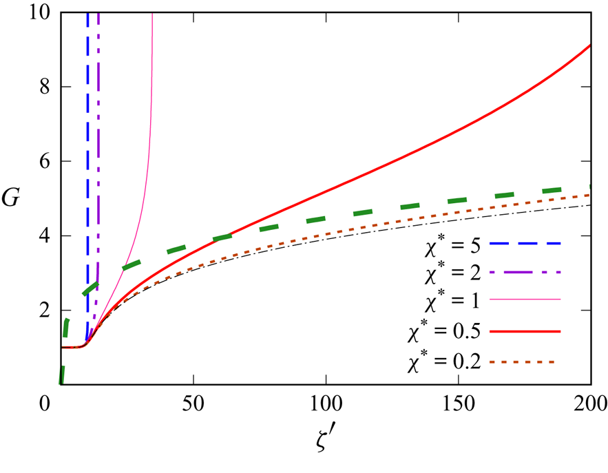
4.1.2. Plots of $G$ vs $\zeta$


In the previous section we plotted  $G$ vs
 $\zeta '$ for the visco-electro-osmotic model for various
 $\chi ^{\ast }$. Of interest also are plots of
 $G$ vs
 $\zeta$ still for the visco-electro-osmotic model where the conversion between
 $\zeta '$ and
 $\zeta$ is given by
 $\zeta \equiv F \zeta '/\Gamma ^{\ast }$ requiring knowledge of the parameters
 $\Gamma ^{\ast }$ and
 $F$, with
 $\chi ^{\ast }$ determining
 $F$ via (2.14). Small
 $\Gamma ^{\ast }$ expands the domain of
 $\zeta$ relative to
 $\zeta '$. Section 2.6.3 suggested to consider
 $\Gamma ^{\ast }$ values down to approximately 0.1; data for that case are plotted in figure 4. Decreasing
 $F$ meanwhile shrinks the domain of
 $\zeta$ relative to
 $\zeta '$. Starting from a value of
 $\chi ^{\ast }=2$ (which is roughly where the maximum for
 $F$ occurs, see § 2.5.2), any change in
 $\chi ^{\ast }$, whether an increase or a decrease, tends to decrease
 $F$. In the case of small
 $\chi ^{\ast }$, however, any shrinkage of the domain of
 $\zeta$ relative to
 $\zeta '$ is more than compensated by an increase in the size of the domain for
 $\zeta '$ itself (as in figure 3). Hence the domain for
 $\zeta$ in the visco-electro-osmotic model actually grows when decreasing
 $\chi ^{\ast }$ from 2 down to 1 down to 0.5 (see figure 4a). For the current case
 $\Gamma ^{\ast }=0.1$, further decreases in
 $\chi ^{\ast }$ below approximately 0.5 are not contemplated here owing to the constraint
 $\Gamma ^{\ast }/|s^{\ast }\sigma _{c0}\sigma _{o0}|\ll \chi ^{\ast \,2}$ imposed in § 3.1.1.
(a) Comparison between  $G$ vs
 $\zeta$ predicted from the full capillary, viscous, electro-osmotic model (thick lines) and the visco-electro-osmotic approximation (thin lines). It is assumed that
 $\Gamma ^{\ast }=0.1$, and
 $\chi ^{\ast }=2$, 1 or 0.5. (b) A zoomed view of the case when
 $\Gamma ^{\ast }=0.1$,
 $\chi ^{\ast }=0.5$.
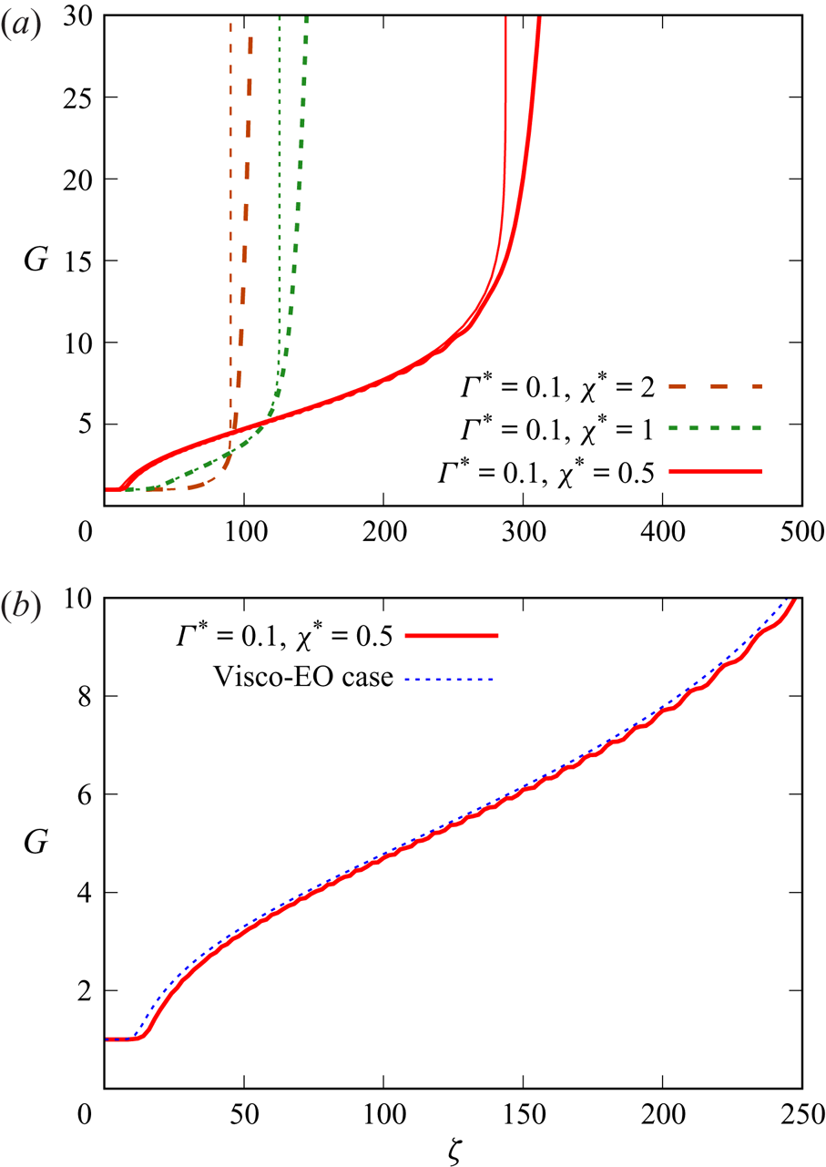
4.1.3. Maximum $\zeta '$ and $\zeta$ values


All visco-electro-osmotic profiles in figures 3 and 4 eventually diverge to infinite  $G$ at some finite maximum
 $\zeta '$ or maximum
 $\zeta$ value. Although this is an artefact of discarding capillary suction from the model, identifying where divergences occur is useful, as it indicates by which point capillary suction terms must be re-inserted.
At small  $\chi ^{\ast }$, the maximum allowed
 $\zeta '$ and/or
 $\zeta$ are predicted to scale as power laws with rapid increases as
 $\chi ^{\ast }$ falls (see § 3.1.3). For our data, a decrease in
 $\chi ^{\ast }$ from 2 down to 1 down to 0.5, turns out to give maximum
 $\zeta$ increasing from 90 to 120 to 280 (assuming
 $\Gamma ^{\ast }=0.1$ here). Further decreases in
 $\chi ^{\ast }$ (giving further increases in maximum
 $\zeta$) would be problematic since § 2.8 estimated that the
 $\zeta$ domain should cover no more than about 1000 units of
 $\zeta$, but are not contemplated in any case, as they violate the constraints needed to admit a visco-electro-osmotic balance (as § 4.1.2 mentions).
Even for combinations of  $\Gamma ^{\ast }$ and
 $\chi ^{\ast }$ that do admit a visco-electro-osmotic balance, an issue still presents itself. Our solution procedure requires us to compute a rescaled film thickness
 $J^{\ast }$ which must be equated to
 $G_{\zeta \zeta ,\infty }\equiv \lim _{\zeta \to \infty } G_{\zeta \zeta }$ yet the visco-electro-osmotic balance already diverges at a finite maximum
 $\zeta$. The electro-osmotic term within (2.5) decays exponentially for
 $G\,\chi ^{\ast }\gg 1$ (see (2.11)) so cannot remain one of the dominant terms in the balance for arbitrarily large
 $G$. To access the large
 $G$ and hence large
 $\zeta$ limiting behaviour of the governing equations, and thereby determine
 $J^{\ast }$, it is essential to return to the full capillary, viscous, electro-osmotic system. This is done in the next section.
4.2. Results for the full capillary, viscous, electro-osmotic system
Sections 4.2.1–4.2.3 that follow examine, for various choices of parameter values, plots of  $G$ vs
 $\zeta$ obtained via the full capillary, viscous, electro-osmotic model. One key finding will be that for small
 $\Gamma ^{\ast }$ and small
 $\chi ^{\ast }$, oscillatory solutions for
 $G$ vs
 $\zeta$ are observed.
4.2.1. Plots of $G$ vs $\zeta$: $\chi ^{\ast }\ge 0.5$


Figure 4(a) plots  $G$ vs
 $\zeta$ data obtained from (2.5) for
 $\Gamma ^{\ast }=0.1$ for a variety of
 $\chi ^{\ast }$ values,
 $\chi ^{\ast }=2$, 1 and 0.5. The trend in figure 4(a) is that any discrepancy between the visco-electro-osmotic model and the full capillary, viscous, electro-osmotic model is pushed towards larger
 $\zeta$ as
 $\chi ^{\ast }$ decreases. Once that discrepancy appears, the visco-electro-osmotic model shows
 $G$ diverging to infinity at finite
 $\zeta$, whereas the full model shows
 $G$ growing, but only attaining arbitrarily large values for arbitrarily large
 $\zeta$. We know that eventually the
 $G$ vs
 $\zeta$ curves for the full model approach parabolas, since
 $G_{\zeta \zeta }$ approaches a well-defined limiting value
 $G_{\zeta \zeta ,\infty }$, which depends on
 $\Gamma ^{\ast }$ and
 $\chi ^{\ast }$. In particular, smaller
 $\chi ^{\ast }$ gives smaller
 $G_{\zeta \zeta ,\infty }$, hence less abrupt growth for
 $G$ in the very large
 $\zeta$ limit. It is only when we zoom in to smaller
 $G$ values within figure 4(b) that we see more structure in the
 $G$ vs
 $\zeta$ solutions. In particular, the
 $\chi ^{\ast }=0.5$ data exhibit a clear inflection point, somewhere below
 $G=2$. Moreover, we see oscillations starting to develop in the
 $\chi ^{\ast }=0.5$ solution. It has already been indicated (see § 3.2) how oscillatory solutions onset in the small
 $\Gamma ^{\ast }$ and small
 $\chi ^{\ast }$ limit. A nominally weak capillary term can balance the electro-osmotic contribution provided oscillations are sufficiently short wavelength.
4.2.2. Oscillatory solutions for $G$ vs $\zeta$: $\chi ^{\ast }=0.2$


To explore the oscillatory solutions further, we continue decreasing the value of  $\chi ^{\ast }$. Figure 5(a) shows a case with
 $\chi ^{\ast }=0.2$ still with
 $\Gamma ^{\ast }=0.1$. Here, we see not only the amplitude of the oscillations gradually growing with
 $\zeta$, but also the wavelength of the oscillations increasing as
 $\zeta$ grows. In the figure, the increase in wavelength is very noticeable when
 $G$ starts exceeding values greater than approximately 20, corresponding to
 $G\,\chi ^{\ast }$ greater than approximately 4. This aligns with what was predicted in § 3.2. Although these are nonlinear oscillations, if we were to linearise (3.8) about some typical
 $G$, we can estimate the wavelength as
 $2\pi (\Gamma ^{\ast }/ (\mathrm {d}T_{\mathit {EO}}/\mathrm {d}G))^{1/2}$ where
 $\mathrm {d}T_{\mathit {EO}}/\mathrm {d}G$ decays exponentially at large
 $G$ (as can be deduced from (2.11).
(a) Oscillatory  $G$ vs
 $\zeta$ computed from the full capillary, viscous, electro-osmotic system (contrasted with the visco-electro-osmotic predictions), for
 $\Gamma ^{\ast }=0.1$ and
 $\chi ^{\ast }=0.2$. Although slightly off the scale of the graph, note that
 $G_{\zeta \zeta }$ changes sign from negative to positive when
 $\zeta$ is slightly above 1800, such that
 $G$ is slightly above 500. Thereafter,
 $G_{\zeta \zeta }$ increases monotonically to a final limiting value
 $\lim _{\zeta \to \infty } G_{\zeta \zeta }\approx 0.00102$. This region was not included on the plot as it involves such large
 $G$ values, that the oscillations (at much smaller
 $G$) would not be visible. (b) Zoomed view of the above.
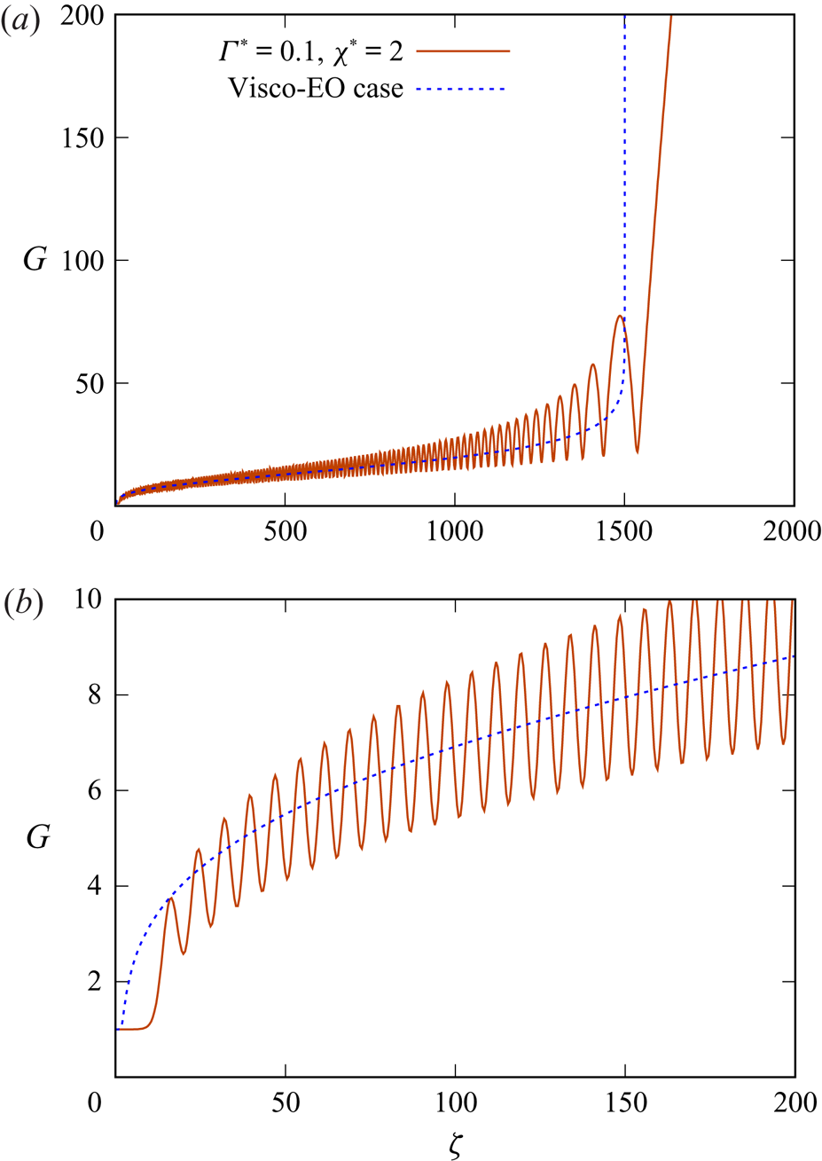
The domain plotted in figure 5(a) actually shows the full set of oscillations in this particular system. By the end of the domain,  $G$ already exceeds 500, so
 $G\,\chi ^{\ast }$ exceeds 100. Electro-osmotic effects are now negligible, so only capillary and possibly viscous terms survive there as per Bretherton (Reference Bretherton1961), and the resulting solutions are non-oscillatory.
What is not shown on figure 5(a), however, is  $G_{\zeta \zeta }$ achieving a final limiting value
 $G_{\zeta \zeta ,\infty }$, as this only occurs for
 $\zeta$ values off the scale of the graph, whereas plotting the graph on much a larger scale would make the oscillations difficult to see. Although data are not plotted here, we have performed the necessary calculation and determined
 $G_{\zeta \zeta ,\infty }\approx 0.00102$ in this case, which is clearly much smaller than the analogous value (
 $J^{\ast }_{{B}}\approx 0.643$) in the system of Bretherton (Reference Bretherton1961).
Even though  $G_{\zeta \zeta ,\infty }$ is positive, the value of
 $G_{\zeta \zeta }$ over the domain from
 $\zeta =1600$ up to approximately
 $\zeta =1800$ is negative as is evident from the curvature of the graph in figure 5(a):
 $G_{\zeta }$ decreases with increasing
 $\zeta$ over this particular domain. Equation (3.9) indicates how a negative
 $G_{\zeta \zeta }$ value can come about in this system. When
 $G$ is very large, electro-osmotic terms are negligible, and hence, according to (3.9),
 $G_{\zeta \zeta }$ is the difference between two small terms, namely
 $G_{\zeta \zeta ,\infty }$ and an integrated term. Since
 $G_{\zeta \zeta ,\infty }\ll 1$, the sign of
 $G_{\zeta \zeta }$ is then sensitive to how the integrated term changes as
 $G$ and
 $\zeta$ vary.
Figure 5(a) thereby underlines the importance of integrating out to sufficiently large  $\zeta$ values when seeking to determine
 $G_{\zeta \zeta ,\infty }\equiv \lim _{\zeta \to \infty }G$ for given
 $\Gamma ^{\ast }$ and
 $\chi ^{\ast }$. It is not possible simply to integrate out to some specified
 $\zeta$ value (e.g.
 $\zeta =1000$) and assume the large
 $\zeta$ limit has been reached. Indeed, as is evident from figure 5(a),
 $\zeta =1000$ is still well within the region where the function is oscillatory. In this oscillatory regime, comparatively small changes in
 $\zeta$ produce large relative changes in
 $G_{\zeta \zeta }$, so
 $G_{\zeta \zeta }$ has definitely not converged to its final limit.
This also impacts on the evaluation of the function  $f$ defined in (2.8). If we stop the integration of (2.5) too soon, such that the integration domain ends whilst
 $G_{\zeta \zeta }$ is still oscillating without having converged to its true final value, then the value of
 $f$ thereby determined will be completely wrong. Evidently evaluating the function
 $f$, and by extension determining its zeroes (see (2.9)), are not always straightforward operations. This is a point to which we will return later.
The fact that this parameter set ( $\Gamma ^{\ast }=0.1$,
 $\chi ^{\ast }=0.2$) requires very large
 $\zeta$ for
 $G_{\zeta \zeta }$ to converge to its final value
 $G_{\zeta \zeta ,\infty }$ raises other considerations as well. Recall that § 2.8 suggested that values of
 $\zeta$ in excess of approximately 1000 need to be treated with caution, since the transition region could start to occupy the entire length of the droplet. It was clarified, however, that this constraint on
 $\zeta$ assumed a
 $J^{\ast }$ value of the order of unity, whereas for a
 $J^{\ast }$ much smaller than unity it should be reasonable to keep
 $\zeta$ less than about
 $1000 \, (J^{\ast })^{-1}$. The present system has
 $J^{\ast }\equiv G_{\zeta \zeta ,\infty }\approx 0.00102$, so the
 $\zeta$ values considered, even those in excess of 1000, do not violate that constraint. Other concerns still arise, however. With a
 $J^{\ast }$ value this small,
 $\bar {\Gamma }$ and
 $\chi '$ values obtained via (2.6) and (2.7) are pushed outside the domain of interest identified in §§ 2.6.1 and 2.6.2. Strictly speaking we should be fixing
 $\bar {\Gamma }$ and
 $\chi '$ (see §§ 4.3 and 4.4 later on) rather than specifying
 $\Gamma ^{\ast }$ and
 $\chi ^{\ast }$.
A further remark on figure 5 concerns comparing data from the full model and the visco-electro-osmotic limit. There is no a priori reason to expect data from these distinct models to be close: when  $\Gamma ^{\ast }=0.1$ and
 $\chi ^{\ast }=0.2$, we are well outside the visco-electro-osmotic model's expected range of validity (
 $\Gamma ^{\ast }/|s^{\ast }\sigma _{c0}\sigma _{o0}| \ll \chi ^{\ast \,2}$ as indicated in § 3.1.1). Nonetheless, it is evident in figure 5 that the visco-electro-osmotic model, whilst not capturing the oscillations of the full model, does manage to track the secular growth of
 $G$, in the event that an average were to be taken over each oscillation cycle.
As well as deviating from the full model for very large  $G$ (i.e.
 $G \,\chi ^{\ast }\gg 1$), the visco-electro-osmotic model also performs particularly poorly for smaller
 $G$ values,
 $G\approx 1$ (see figure 5b). We know from § 2.7 that
 $G-1$ grows exponentially like
 $\exp (\Lambda \,\zeta )$. For the current
 $\Gamma ^{\ast }$ and
 $\chi ^{\ast }$ values, the full model predicts
 $\Lambda \approx 1$ whereas the visco-electro-osmotic model predicts
 $\Lambda =\Gamma ^{\ast }/F$, which for the current
 $\Gamma ^{\ast }$ and
 $\chi ^{\ast }$ corresponds to an overestimate of the true growth rate.
Notice also that, even though the predictions for the growth rates differ, the full model is still exponential, and hence non-oscillatory, at first. In figure 5(a) no oscillation is seen for  $G$ values between 1 and 3 approximately. This behaviour follows from
 $\mathrm {d}T_{\mathit {EO}}/\mathrm {d}G$ being small when its argument
 $G\,\chi ^{\ast }$ is small, thereby weakening the electro-osmotic term in (2.5). The dominant balance for
 $G$ values between about 1 and 3 is therefore between capillary and viscous terms as in the classical Bretherton (Reference Bretherton1961) system (indeed
 $\Lambda \equiv 1$ identically in that classical system).
4.2.3. Oscillatory solutions for $G$ vs $\zeta$: $\chi ^{\ast }=0.1$ and $\chi ^{\ast }=0.02$


Figure 6 plots data for two more  $\chi ^{\ast }$ values, namely
 $\chi ^{\ast }=0.1$ and
 $\chi ^{\ast }=0.02$. Clearly the solutions are oscillatory. The plot shows only a restricted domain of
 $\zeta$ values, and does not attempt to show the oscillations eventually coming to an end, with
 $G$ then growing indefinitely, and
 $G_{\zeta \zeta }$ approaching some final value
 $G_{\zeta \zeta ,\infty }$. Even within this restricted domain, however, we can observe differences between the
 $\chi ^{\ast }=0.1$ and
 $\chi ^{\ast }=0.02$ cases.
Oscillatory  $G$ vs
 $\zeta$ for
 $\Gamma ^{\ast }=0.1$ with
 $\chi ^{\ast }=0.1$ and
 $\chi ^{\ast }=0.02$. This zoomed view only plots a limited domain of
 $\zeta$, but the oscillations themselves persist out to much larger
 $\zeta$.

For  $\chi ^{\ast }=0.1$ oscillations are much shorter wavelength, and smaller amplitude. In this case, the oscillations vary between about
 $G\approx 10$ to
 $G\approx 20$, so
 $G\,\chi ^{\ast }$ varies between 1 and 2. The oscillations seem to select the region where
 $\mathrm {d}T_{\mathit {EO}}/\mathrm {d}G$ is largest, recalling from (2.13), that the maximum occurs for
 $G\,\chi ^{\ast }\approx 1.316$. Keeping
 $\mathrm {d}T_{\mathit {EO}}/\mathrm {d}G$ as large as possible helps to keep the wavelength short, as § 3.2.1 mentions.
In the case  $\chi ^{\ast }=0.02$, the oscillations cover the range from approximately
 $G=10$ up to almost
 $G=100$, and hence
 $G\,\chi ^{\ast }$ ranges roughly from 0.2 up to 2. It follows that the amplitude of the oscillations in
 $G$ must scale roughly like
 $1/\chi ^{\ast }$. The
 $G$ value with maximal
 $\mathrm {d}T_{\mathit {EO}}/\mathrm {d}G$ (namely
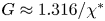 $G\approx 1.316/\chi ^{\ast }$) is still contained within the range of oscillation, but since the maximal
 $\mathrm {d}T_{\mathit {EO}}/\mathrm {d}G$ is sensitive to
 $\chi ^{\ast }$ (see (2.13)), reducing
 $\chi ^{\ast }$ tends to increase wavelength, which (see §§ 3.2.1 and 4.2.2) scales proportional to
 $(\mathrm {d}T_{\mathit {EO}}/\mathrm {d}G)^{-1/2}$.
In summary then, (2.5) incorporating attractive electro-osmotic interactions admits oscillatory solutions, even at the front of the droplet, a contrast with the classical case of Bretherton (Reference Bretherton1961) which does not admit oscillations at the front, only at the rear. For the oscillations to appear, the parameter  $\Gamma ^{\ast }$ must be small and
 $\chi ^{\ast }$ must also be small. Increasing
 $\chi ^{\ast }$ tends to reduce the amplitude of the oscillations and eventually suppresses them altogether, which is understandable, since increasing
 $G\,\chi ^{\ast }$ significantly above unity weakens the electro-osmotic interactions owing to charge screening.
What we do not yet know, however, is whether a system with realistic parameter values ever actually selects such solutions. The reason this is still unknown is that the parameters we are normally given are not  $\Gamma ^{\ast }$ and
 $\chi ^{\ast }$ but rather
 $\bar {\Gamma }$ and
 $\chi '$. Using given
 $\bar {\Gamma }$ and
 $\chi '$ values, we must solve (2.9) to obtain
 $J^{\ast }$ and only then are
 $\Gamma ^{\ast }$ and
 $\chi ^{\ast }$ obtained via (2.6) and (2.7). Solutions for (2.9) are presented in the next two sections.
4.3. Data for $J^{\ast }$ for $\bar {\Gamma }=10$ and $\bar {\Gamma }=1$


Section 2.6 suggested a base case value of  $\bar {\Gamma }=10$ but also stated that
 $\bar {\Gamma }$ could fall as low as
 $\bar {\Gamma }=0.1$ for an increased density of charge adsorption sites. The smaller the value of
 $\bar {\Gamma }$, the more significant the electro-osmotic interactions. In the present section we consider the case of weak to moderate strength electro-osmotic interactions
 $\bar {\Gamma }=10$ and
 $\bar {\Gamma }=1$, with the case of stronger interactions
 $\bar {\Gamma }=0.1$ (which turns out to be rather more complicated) being considered in § 4.4.
For the case  $\bar {\Gamma }=10$, data for
 $J^{\ast }$ vs
 $\chi '$ (determining
 $J^{\ast }$ as the solution of (2.9)) are plotted in figure 7(a). Similar data, specific to the case
 $\bar {\Gamma }=10$, have already been presented by Grassia (Reference Grassia2019). The domain of
 $\chi '$ plotted is as suggested in § 2.6, namely
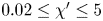 $0.02\le \chi '\le 5$, spanning the domain from low speed, low salinity floods (no charge screening) to high speed, high salinity floods (strongly screened charges). As
 $\chi '$ decreases,
 $J^{\ast }$ migrates from around
 $J^{\ast }_{{B}}\approx 0.643$ to a lower value. Since
 $J^{\ast }$ represents film thickness we deduce that the attractive electro-osmotic interactions being considered in this case cause the film to thin, as we expect. That said the film thinning is comparatively modest, at most approximately 10 %, a strong contrast with the orders of magnitude of film thickening seen for repulsive interactions in Grassia (Reference Grassia2019). Films must thicken significantly in the repulsive case, as otherwise electro-osmotic tension would diverge (Grassia Reference Grassia2019). However, in the attractive case, there are only very gradual changes in the electro-osmotic pressure for comparatively thin films: see e.g. figure 2. This in turn limits the impact that gradients of electro-osmotic tension have upon (2.5) keeping solutions of that equation comparatively close to those from the uncharged case.
Computed  $J^{\ast }$ vs
 $\chi '$ for (a)
 $\bar {\Gamma }=10$ and (b)
 $\bar {\Gamma }=1$. Here the computed
 $J^{\ast }$ is required to satisfy (2.9). The approximate formula for estimating
 $J^{\ast }$, (3.14), is also shown (dashed curve). The horizontal lines represent, respectively, the classical Bretherton (Reference Bretherton1961) value
 $J^{\ast }_{{B}}$ (which is the
 $\chi '\to \infty$ limit of (3.14)) and also the
 $\chi '\to 0$ limit of (3.14) which matches (3.12).

In the limit of small  $\chi '$, the estimate for
 $J^{\ast }$ via (3.12) is borne out very well. Remembering from § 2.4 that the parameter
 $|s^{\ast } \sigma _{c0}\sigma _{o0}|$ in (3.12) is set to unity, and that
 $\bar {\Gamma }=10$, this explains the 10 % change seen in
 $J^{\ast }$ between the large
 $\chi '$ and small
 $\chi '$ limits. This suggests that the physical picture described in § 3.3.1 is valid. Thus in the
 $\chi '\ll 1$ limit, there should be a subdomain with
 $G\ll 1/\chi ^{\ast }$ within which a classical capillary, viscous balance applies, so that for values
 $G$ satisfying
 $1\ll G\ll 1/\chi ^{\ast }$, the value of
 $G_{\zeta \zeta }$ computed by (2.5) approaches
 $J^{\ast }_{{B}}$. Then for
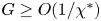 $G\ge O(1/\chi ^{\ast })$, the value of
 $G_{\zeta \zeta }$ adjusts via a capillary, electro-osmotic balance, falling from
 $J^{\ast }_{{B}}$ down to a
 $J^{\ast }$ value as plotted in figure 7(a), itself approximately 10 % lower than
 $J^{\ast }_{{B}}$.
As well as being able to estimate  $J^{\ast }$ in the small and large
 $\chi '$ limits, we also have an ad hoc formula estimating it at all
 $\chi '$ values, namely (3.14). Figure 7(a) shows that this formula captures the trend of the numerical
 $J^{\ast }$ data, but for intermediate
 $\chi '$ the data are underestimated. In § 3.4.1 we actually anticipated that (3.14) might overestimate the data. Since this expectation is not borne out, we need to challenge some of the assumptions used to derive (3.14), a key assumption having been that a viscous contribution to
 $G_{\zeta \zeta }$ would always integrate roughly to
 $J^{\ast }_{{B}}$ regardless of
 $\chi '$.
Figure 7(b) shows data for  $J^{\ast }$ for the case
 $\bar {\Gamma }=1$. Qualitatively, the data are similar to those in figure 7(a) the main difference being that
 $J^{\ast }$ now changes much more substantially, the small
 $\chi '$ value of
 $J^{\ast }$ being about half the value found at large
 $\chi '$. This is exactly in line with what (3.12) suggests. Moreover, the ad hoc formula (3.14) seems to capture reasonably well how
 $J^{\ast }$ varies with
 $\chi '$, although once again yields a slight underestimate (seen clearly for the data point at
 $\chi '=5$).
This completes our analysis for  $\bar {\Gamma }=10$ and
 $\bar {\Gamma }=1$. In the next section we study a case with stronger electro-osmotic effects
 $\bar {\Gamma }=0.1$, which proves to be rather more complex.
4.4. Data for $\bar {\Gamma }=0.1$

The discussion for a system with  $\bar {\Gamma }=0.1$ is divided into several parts. First we investigate profiles of
 $f(J^{\ast })$ vs
 $J^{\ast }$, for relatively large
 $\chi '$ values (§ 4.4.1). Then we do the same for smaller
 $\chi '$ values (§§ 4.4.2 and 4.4.3). After that we consider the
 $J^{\ast }$ values satisfying (2.9)) for various
 $\chi '$ (§ 4.4.4). Finally we explore profiles of
 $G$ vs
 $\zeta$ and
 $G_{\zeta \zeta }$ vs
 $\zeta$ (§§ 4.4.5–4.4.7). Key findings will be that, for certain combinations of
 $\bar {\Gamma }$ and
 $\chi '$, multiple solutions for
 $J^{\ast }$ (i.e. multiple solutions for film thickness) are admitted, some of these having non-oscillatory
 $G$ vs
 $\zeta$ profiles, and others having oscillatory profiles.
4.4.1. Data for $f(J^{\ast })$ vs $J^{\ast }$


In figure 8(a) we plot  $f(J^{\ast })$ vs
 $J^{\ast }$ for
 $\bar {\Gamma }=0.1$ and various
 $\chi '$ values, from
 $\chi '=9$ down to
 $\chi '=2$. Although we are mostly interested in values of
 $\chi '\le 5$ here (see § 2.6), it is instructive to include some slightly larger
 $\chi '$ values, because increasing
 $\chi '$ is a way of shifting the system closer to the classical state of Bretherton (Reference Bretherton1961). Another way of approaching that state is of course increasing
 $\bar {\Gamma }$, but
 $\bar {\Gamma }$ remains fixed at 0.1 here.
The function  $f(J^{\ast })$ vs
 $J^{\ast }$: the zeroes of
 $f(J^{\ast })$ are sought. (a) The case
 $\bar {\Gamma }=0.1$ and
 $\chi '=9$, 8, 5 and 2. (b) Zoomed view of (a). (c) The case
 $\bar {\Gamma }=0.1$ and
 $\chi =2$, 0.2 and 0.02.

The data for  $\chi '=9$ show that
 $f(J^{\ast })$ has a zero for
 $J^{\ast }$ just slightly above 0.6. This then indicates a prediction for
 $J^{\ast }$ close to the value
 $J^{\ast }_{{B}}\approx 0.643$. However, the data for
 $\chi '=9$ show that
 $f(J^{\ast })$ also has a local minimum for
 $J^{\ast }$ just slightly below 0.1. This is clear in the zoomed view in figure 8(b). The
 $f$ value at the local minimum is greater than zero, so for
 $\chi '=9$, the only solution for
 $f(J^{\ast })=0$ remains the one with
 $J^{\ast }$ greater than 0.6, i.e. the state remains close to the classical case of Bretherton (Reference Bretherton1961).
For  $\chi '=8$, however, the behaviour changes. The local minimum now falls to a value with
 $f<0$. This means there are now three solutions for
 $J^{\ast }$ satisfying
 $f=0$ (as per (2.9)), one with a
 $J^{\ast }$ value that is still around 0.6, and another two
 $J^{\ast }$ values around 0.1 and 0.07, respectively. Since
 $J^{\ast }$ represents the film thickness, this means that, for this
 $\bar {\Gamma }$ and
 $\chi '$ combination there are three different solutions for the film thickness, each having different
 $\Gamma ^{\ast }$ and
 $\chi ^{\ast }$ values and hence a different
 $G$ vs
 $\zeta$ profile. The analysis does not tell us which of those three solutions is stable, as the derivation of (2.5) merely assumed the existence of a steady state
 $G$ vs
 $\zeta$ profile in the frame of reference of the droplet, and did not address questions of stability.
As  $\chi '$ decreases below
 $\chi '=8$, the
 $J^{\star }$ value corresponding to each of the three branches of solutions migrates as
 $\chi '$ falls. Nonetheless, when
 $\chi '=5$, we can still recognise the same three branches of solutions as at
 $\chi '=8$; however, the largest of the three solutions has now fallen to a
 $J^{\ast }$ value close to 0.1. Although this is the same branch of solutions that joins up with the classical solution with
 $J^{\ast }\to J^{\ast }_{{B}}$ at sufficiently large
 $\chi '$, in the case of
 $\chi '=5$, the
 $J^{\ast }$ value has already migrated far away from
 $J^{\ast }_{{B}}$.
4.4.2. Effect upon $f(J^{\ast })$ vs $J^{\ast }$ of decreasing $\chi '$


A further decrease in  $\chi '$ down to
 $\chi '=2$ still with
 $\bar {\Gamma }=0.1$ reveals even more structure in the
 $f(J^{\ast })$ vs
 $J^{\ast }$ plot in figure 8(a,b). When
 $\chi '=2$ the plot for
 $f$ vs
 $J^{\ast }$ has as many as five maxima and minima, but much of this structure is seen at
 $f$ values well below zero, and hence does not affect the determination of the roots of
 $f$. That said, there are now five solutions for
 $f(J^{\ast })=0$, the same three branches as identified for
 $\chi '=5$ and
 $\chi '=8$, plus two new branches located either side of a local maximum of
 $J^{\ast }$ close to
 $J^{\ast }\approx 0.1$. In the interest of simplicity, we will not consider the fourth and fifth solution branches any further in what follows, since for the arguments we need to make, it is sufficient to consider just three branches.
By referring to the analysis of §§ 3.2 and 3.3, it is possible to explain why  $f(J^{\ast })$ develops this complex structure. There are two parts to the explanation below. First we explain the general shape of the
 $f(J^{\ast })$ vs
 $J^{\ast }$ curve ignoring the oscillations, and then we explain why oscillations are superposed on that general shape.
The function  $f$ is the difference between
 $G_{\zeta \zeta ,\infty }$ and
 $J^{\ast }$, so to understand the general shape of the
 $f$ vs
 $J^{\ast }$ curve, it is sufficient to analyse the general behaviour of
 $G_{\zeta \zeta ,\infty }$. Remember that as we increase
 $J^{\ast }$ for fixed
 $\bar {\Gamma }$ and fixed
 $\chi '$ we are decreasing
 $\Gamma ^{\ast }$ via (2.6) but increasing
 $\chi ^{\ast }$ via (2.7). The fact that
 $\Gamma ^{\ast }$ decreases indicates in (2.5) that electro-osmotic interactions are effectively becoming stronger. We are dealing with attractive interactions here, so (as we argued in § 2.3) we expect
 $G_{\zeta \zeta ,\infty }$ to be smaller than
 $J^{\ast }_{{B}}$. Moreover,
 $G_{\zeta \zeta ,\infty }$ should decrease as electro-osmotic interactions strengthen with increasing
 $J^{\ast }$ (i.e. with decreasing
 $\Gamma ^{\ast }\equiv \bar {\Gamma }/J^{\ast }$).
In fact  $G_{\zeta \zeta ,\infty }$ decreases quite rapidly at first with increasing
 $J^{\ast }$, since it can be estimated by (3.11), which applies as long as
 $\chi ^{\ast }$ is small, which certainly will be the case for small
 $J^{\ast }$ at fixed
 $\chi '$ (see (2.7)). Equation (3.11) then implies that
 $G_{\zeta \zeta ,\infty }$ will decrease from
 $J^{\ast }_{{B}}$ when
 $J^{\ast }=0$ to some value
 $G_{\zeta \zeta ,\infty }\ll J^{\ast }_{{B}}$ when
 $J^{\ast }$ reaches a value of the order of
 $J^{\ast }_{{B}}\, \bar {\Gamma }/|s^{\ast }\sigma _{c0}\sigma _{o0}|$. Once
 $G_{\zeta \zeta ,\infty }$ attains a value much smaller than
 $J^{\ast }_{{B}}$ we anticipate that its value will remain small thereafter even if
 $J^{\ast }$ is increased further. As mentioned above, the effect of increasing
 $J^{\ast }$ is to decrease
 $\Gamma ^{\ast }$, making electro-osmotic interactions more significant within (2.5). Since
 $G_{\zeta \zeta ,\infty }$ represents a film thickness, and since we are dealing with attractive electro-osmotic interactions here, the films should stay much thinner than the case of Bretherton (Reference Bretherton1961).
Thus, ignoring any oscillatory behaviour, the general form of the function  $G_{\zeta \zeta ,\infty }$ vs
 $J^{\ast }$ is expected to be a sharp decrease over a small
 $J^{\ast }$ range, followed by
 $G_{\zeta \zeta ,\infty }$ staying relatively small for further increases in
 $J^{\ast }$. As a consequence, the general form of
 $f\equiv G_{\zeta \zeta ,\infty }-J^{\ast }$ vs
 $J^{\ast }$ must be a sharp decrease followed by a more gradual decrease. This is what figure 8 shows, at least ignoring the oscillations.
Now we consider the oscillations in  $f$. For
 $\chi '=2$, these appear (see figure 8a,b) as occasional step increases in
 $f$ superposed on the overall decreasing trend for
 $f$ as discussed above. We already know that if we manage to find a regime in which
 $\Gamma ^{\ast }$ is significantly smaller than unity, whilst
 $\chi ^{\ast }$ is also small, we expect to find oscillatory solutions for
 $G$ vs
 $\zeta$. As we saw in § 4.2, depending on the values of
 $\Gamma ^{\ast }$ and
 $\chi ^{\ast }$, different numbers of oscillations are possible in the
 $G$ vs
 $\zeta$ profile, after which at large enough
 $\zeta$, the value of
 $G$ begins growing definitively without further oscillation. Moreover, each additional oscillation added to the
 $G$ vs
 $\zeta$ profile, implies
 $G$ must migrate once more from a local maximum to a local minimum. Whenever
 $G$ approaches a local minimum, however, we expect to see an increment in the value of
 $G_{\zeta \zeta ,\infty }$. The reason for this is discussed already in § 3.2.2: increases in
 $G_{\zeta \zeta }$ are driven by an integrated term in (3.9) and/or (3.10)) which is most active when
 $G$ is smaller, and less active when
 $G$ is larger. Thus superposed on the general tendency of
 $f(J^{\ast })$ to decrease as
 $J^{\ast }$ increases, we see occasional increases in
 $f(J^{\ast })$ leading overall to oscillations in
 $f$ vs
 $J^{\ast }$.
4.4.3. Abruptness of increases in $f(J^{\ast })$ vs $J^{\ast }$


The analysis just presented also explains another feature evident as we move to yet smaller  $\chi '$ in figure 8(c), namely why the increase in
 $f$ from a local minimum to a local maximum is abrupt when either
 $\chi '$ or
 $J^{\ast }$ or both are small (hence giving small
 $\chi ^{\ast }\equiv J^{\ast }\chi '$) but nowhere near so abrupt for larger
 $\chi '$ and/or larger
 $J^{\ast }$. In § 4.2.2, oscillations in
 $G$ vs
 $\zeta$ were seen to be large amplitude when
 $\chi ^{\ast }$ was small, the amplitude of the oscillation scaling roughly as
 $1/\chi ^{\ast }$. For a small
 $\chi ^{\ast }$, large amplitude oscillation,
 $G$ spends most of the oscillation cycle with values
 $G\sim O(1/\chi ^{\ast })\gg 1$, only attaining
 $G$ values of order unity right near the minimum of the oscillation. The integral term on the right-hand side of (3.9) and (3.10) is therefore completely inactive except when
 $G$ is at or near the minimum of the oscillation.
Based on this behaviour within (3.9) and (3.10), it follows that an abrupt almost step-like increase in  $G_{\zeta \zeta ,\infty }$ and hence in
 $f$ is associated with a bifurcation between different
 $G$ vs
 $\zeta$ profiles. Two systems with almost the same
 $\Gamma ^{\ast }$ and
 $\chi ^{\ast }$ will have
 $G$ vs
 $\zeta$ profiles remaining very close to each other during a given number of oscillation cycles, but at some point one profile manages to stop oscillating to diverge to infinity, while the other undergoes one extra oscillation before diverging. Since each oscillation in
 $G$ increases the eventual final value of
 $G_{\zeta \zeta }$ (see the discussion following (3.10)), the profile that undergoes the extra oscillation ends up with the larger
 $G_{\zeta \zeta ,\infty }$ value. Hence even though that profile oscillates for longer before starting to diverge, it must eventually overtake a profile that stopped oscillating sooner, but which grows with a smaller
 $G_{\zeta \zeta ,\infty }$.
To summarise, oscillations seen in the  $f(J^{\ast })$ vs
 $J^{\ast }$ profiles in figure 8 mirror differing numbers of oscillations in the
 $G$ vs
 $\zeta$ profiles (§ 4.2) as
 $\Gamma ^{\ast }$ falls via (2.6) and
 $\chi ^{\ast }$ rises via (2.7) for increasing
 $J^{\ast }$ but fixed
 $\bar {\Gamma }$ and
 $\chi '$. Each new oscillation added to the
 $G$ vs
 $\zeta$ profile implies an oscillation in
 $f$ vs
 $J^{\ast }$. Moreover, when
 $\chi '$ is small, many oscillations can be expected in
 $G$ vs
 $\zeta$, and hence in
 $f$ vs
 $J^{\ast }$ (see e.g. figure 8c). Note that adding one extra oscillation onto an already highly oscillatory
 $G$ vs
 $\zeta$ is expected to have little impact on the value of
 $G_{\zeta \zeta ,\infty }$. As a result, the amplitude of oscillations in
 $f$ vs
 $J^{\ast }$ tends to decay with successive oscillations (again see figure 8c).
4.4.4. Data for $J^{\ast }$ vs $\chi '$


In the previous section we examined graphs of  $f(J^{\ast })$ vs
 $J^{\ast }$ for fixed
 $\bar {\Gamma }=0.1$ and various
 $\chi '$, and explained how the shapes of those graphs came about. In the present section we examine, still for
 $\bar {\Gamma }=0.1$, graphs of
 $J^{\ast }$ (specifically the
 $J^{\ast }$ values satisfying (2.9)) as functions of
 $\chi '$.
What we see in figure 9(a) is that for sufficiently large  $\chi '$, the system approaches the value
 $J^{\ast }_{{B}}\approx 0.643$, although we have to go to
 $\chi '$ values of approximately 10 to see this, whereas in § 2.6 we established that values of
 $\chi '$ are likely to be somewhat smaller than this, e.g.
 $\chi '\approx 5$ corresponds to a high speed, high salinity flood. As
 $\chi '$ falls we see in figure 9(a) that the value of
 $J^{\ast }$ falls quite sharply, certainly more sharply than our ad hoc approximation (3.14) suggests. Moreover, in the limit
 $\chi '\ll 1$ (such as we might encounter for a low speed, low salinity flood), the
 $J^{\ast }$ value fails to match the estimate via (3.12). This is a concern as (3.12) was derived under a mild set of assumptions, namely that a classical capillary, viscous balance applies in a subdomain
 $1\le G\ll 1/\chi ^{\ast }$ whereas a capillary, electro-osmotic balance applies for
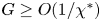 $G\ge O(1/\chi ^{\ast })$ and causes the
 $G_{\zeta \zeta }$ value to adjust from
 $J^{\ast }_{{B}}$ down to a smaller value.
(a) Computed  $J^{\ast }$ vs
 $\chi '$ vs in the case
 $\bar {\Gamma }=0.1$. Here, the computed
 $J^{\ast }$ is required to satisfy (2.9). The dashed line shows the approximate formula
 $J^{\ast }$, (3.14), and the horizontal line is (3.12). (b) Zoomed view of (a) showing three branches of solutions, a branch with the largest
 $J^{\ast }$ (which extends all the way to
 $\chi '\to \infty$), and branches with intermediate and smallest
 $J^{\ast }$ values, which only appear for
 $\chi '$ smaller than about 8.

What figure 9(a) overlooks, however, is that the  $J^{\ast }$ value satisfying (2.9) is not necessarily unique. As is clear from figure 8(b), two new solution branches appear for
 $\chi '$ values less than approximately 8. Figure 9(b) is a zoomed view of figure 9(a) showing three solution branches, the original branch, plus two new ones. Since
 $J^{\ast }$ physically represents film thickness here, the different solution branches correspond to different thickness films. It is clear that that the solution with the smallest
 $J^{\ast }$ (i.e. with the thinnest film) is the one that agrees with (3.12) in the small
 $\chi '$ limit. This then must be the solution that obeys a capillary, viscous balance for small
 $G\,\chi ^{\ast }$ values but a capillary, electro-osmotic balance for larger
 $G\,\chi ^{\ast }$.
On the basis of the above results, we can now summarise the regimes of behaviour we expect. If  $\bar {\Gamma }\gg 1$ (or strictly speaking if
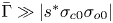 $\bar {\Gamma }\gg |s^{\ast }\sigma _{c0}\sigma _{o0} |$, with
 $|s^{\ast }\sigma _{c0}\sigma _{o0} |\equiv 1$ in the present study) then we expect that
 $J^{\ast }\approx J^{\ast }_{{B}}$ regardless of the value of
 $\chi '$ (figure 7(a) is a case in point). Moreover, if
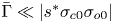 $\bar {\Gamma }\ll |s^{\ast }\sigma _{c0}\sigma _{o0} |$, but
 $\chi '\gg |s^{\ast }\sigma _{c0}\sigma _{o0} |/( J^{\ast }_{{B}} \bar {\Gamma })$, then we again anticipate that
 $J^{\ast }$ will be close to
 $J^{\ast }_{{B}}$. On the other hand if
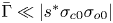 $\bar {\Gamma }\ll |s^{\ast }\sigma _{c0}\sigma _{o0} |$ and
 $\chi '$ is sufficiently small, i.e. provided
 $\chi '\ll |s^{\ast }\sigma _{c0}\sigma _{o0} |/( J^{\ast }_{{B}} \bar {\Gamma })$, then (3.12) can be applied and in fact reduces to
 \begin{equation} J^{\ast} \approx J^{\ast}_{{B}} \bar{\Gamma}/|s^{\ast}\sigma_{c0}\sigma_{o0} | \end{equation}
in this limit. The domain in which (4.1) applies is also the regime in which multiple solutions for  $J^{\ast }$ are possible, with (4.1) capturing just the smallest of those multiple
 $J^{\ast }$ solutions.
4.4.5. Data for $G$ vs $\zeta$: large $\chi '$ case, $\chi '=5$


In order to understand how multiple branches of solutions each with different  $J^{\ast }$ can come about, it is instructive to examine profiles of
 $G$ vs
 $\zeta$ corresponding to each branch. In figure 10 we do this for
 $\bar {\Gamma }=0.1$ and
 $\chi '=5$, this
 $\chi '$ value being considered ‘large’ in the sense that (according to § 2.6.2) it is towards the upper end of the domain of
 $\chi '$ of interest. What we see in figure 10 is that a difference starts appearing between the profiles around
 $\zeta \approx 10$, the profile with the smallest
 $J^{\ast }$ having a monotonically increasing
 $G$, but the profile with the largest
 $J^{\ast }$ undergoing an oscillation,
 $G$ having first a local maximum, then a local minimum, and after that increasing without further oscillation.
Predicted  $G$ vs
 $\zeta$ obtained from the full capillary, viscous, electro-osmotic system for
 $\bar {\Gamma }=0.1$,
 $\chi '=5$ and three different solution branches for
 $J^{\ast }$. All three of these
 $J^{\ast }$ values satisfy (2.9).

The branch with the intermediate  $J^{\ast }$ has a different behaviour. Initially it stays close to the branch with smallest
 $J^{\ast }$, but around
 $\zeta \approx 20$, it exhibits an inflection point. The rate of increase of
 $G$ becomes increasingly slow. At larger
 $\zeta$ this branch exhibits a local maximum in
 $G$ (off the scale of the graph at a value roughly
 $\zeta \approx 60$), followed by a local minimum (again off the scale at roughly
 $\zeta \approx 120$), followed by an increase without further oscillation. Qualitatively speaking then the
 $G$ vs
 $\zeta$ shape for the branch with intermediate
 $J^{\ast }$ is therefore similar to the shape for the branch with the largest
 $J^{\ast }$. What is different, however, is the location of the maximum and minimum, which are pushed out to much larger
 $\zeta$ values for the intermediate
 $J^{\ast }$ branch.
We have already discussed (see §§ 2.3, 3.2.2 and 4.4.2) that the general trend is for  $f$ to decrease as
 $J^{\ast }$ increases, but intermittent increases in
 $f$ are possible, associated with a solution managing to add an extra oscillation to the
 $G$ vs
 $\zeta$ profile. The borderline between a solution that narrowly fails to add an extra oscillation and one that just manages to do so, is a solution that ‘dithers’, in other words, it stays at comparatively large
 $G$ for a comparatively wide domain of
 $\zeta$ values before
 $G$ either definitively increases or else oscillates. The intermediate branch of
 $J^{\ast }$ values corresponds therefore to one such ‘dithering’ solution. This makes it challenging to compute this particular solution branch numerically. By its nature, the solution needs to reach large
 $\zeta$ values before settling into any definitive limiting behaviour: we need to follow
 $G$ vs
 $\zeta$ for quite some distance before the limiting value
 $G_{\zeta \zeta ,\infty }$ is attained. On the other hand we need to know that limiting behaviour before we can solve (2.9) and identify the correct
 $J^{\ast }$ in the first place.
This is underlined by the behaviour of these functions at very large  $\zeta$ (well off the scale of figure 10). Via (2.9), we know that
 $G_{\zeta \zeta ,\infty }=J^{\ast }$, so that systems with larger
 $J^{\ast }$ necessarily have faster growing
 $G$ in the large
 $\zeta$ limit. Whereas the branch with the largest
 $J^{\ast }$ already has the largest
 $G$ value by
 $\zeta =100$, the
 $G$ value for the intermediate
 $J^{\ast }$ branch only manages to overtake the branch with the smallest
 $J^{\ast }$ when
 $\zeta$ is well over 1000. We have already flagged up issues (see § 2.8) with taking solutions to excessively large
 $\zeta$ values: if
 $\zeta$ becomes too large, the transition region that we are computing between the thin film region and capillary static region may well grow to become comparable with the length of the droplet as a whole.
4.4.6. Data for $G$ vs $\zeta$: small $\chi '$ case, $\chi '=0.02$


In the present section we show data analogous those in the previous section, except that previously we considered a comparatively large  $\chi '$ value (
 $\chi '=5$), and here we consider a much smaller
 $\chi '$ value (
 $\chi '=0.02$, a ‘small’ value, identified in § 2.6.2 as being towards lower end of the domain of interest for
 $\chi '$). Results are plotted in figure 11.
(a) Value of  $G$ vs
 $\zeta$ for
 $\bar {\Gamma }=0.1$,
 $\chi '=0.02$ and three different solution branches for
 $J^{\ast }$; (b)
 $G_{\zeta \zeta }$ vs
 $\zeta$ for
 $\bar {\Gamma }=0.1$,
 $\chi '=0.02$ and three branches for
 $J^{\ast }$.

Qualitatively, the findings are similar to figure 10. Of the three solution branches, the one with the smallest  $J^{\ast }$ is a branch for which
 $G$ is monotonically increasing. The solution branch with the largest
 $J^{\ast }$ exhibits an oscillation: there is exactly one local maximum followed by one local minimum, after which the solution begins increasing definitively. However, the local maximum and local minimum are now at much larger
 $\zeta$ values than was the case in figure 10. Moreover the difference in
 $G$ between the local maximum and local minimum is striking. The local maximum has
 $G$ in excess of 5000, whilst the local minimum (although difficult to see on the scale of the graph) has
 $G$ slightly less than 5. The maximum has a
 $G$ value of the order of
 $1/\chi ^{\ast }\equiv 1/(\chi ' J^{\ast })\gg 1$ whilst the minimum has a
 $G$ value back down to order unity: the amplitude of the oscillation therefore scales like
 $1/\chi ^{\ast }$ similar to what was seen in § 4.2.3.
The solution branch with intermediate  $J^{\ast }$ seems to be borderline between the two types of behaviour aforementioned. In figure 11(a), the graph of
 $G$ vs
 $\zeta$ for this branch appears to be close to a straight line for a large part of the solution domain. Hence, it is unclear from the shape of the graph if the solution for
 $G$ will ultimately continue growing indefinitely (as per the smallest
 $J^{\ast }$ case) or will eventually, at extremely large
 $\zeta$, undergo an oscillation as per the largest
 $J^{\ast }$ branch. This solution therefore represents a bifurcation between a non-oscillatory and oscillatory
 $G$. Although the ultimate fate of the solution can be decided by taking it to very large
 $\zeta$, well in excess
 $\zeta =1000$ plotted here, there comes a point at which it becomes meaningless to do that: as commented in the previous section, the branch with intermediate
 $J^{\ast }$ is inherently difficult to calculate.
4.4.7. Data for $G_{\zeta \zeta }$ vs $\zeta$ vs $\zeta$: small $\chi '$ case, $\chi '=0.02$


More insights into the small  $\chi '$ solutions just discussed can be gained by considering plots for
 $G_{\zeta \zeta }$ vs
 $\zeta$. In the case of the solution with the smallest
 $J^{\ast }$, the behaviour is exactly as predicted in § 3.3.1, namely
 $G_{\zeta \zeta }$ rises from 0 to
 $J^{\ast }_{{B}}\approx 0.643$ and then falls back to a limiting value
 $G_{\zeta \zeta ,\infty }$ which is much smaller than
 $J^{\ast }_{{B}}$. In the case of the solution with the largest
 $J^{\ast }$, the initial shape of the
 $G_{\zeta \zeta }$ profile is similar. It rises to a maximum with a value of
 $G_{\zeta \zeta }$ roughly
 $J^{\ast }_{{B}}$ at the maximum, and then falls after that. However, it now falls to a negative
 $G_{\zeta \zeta }$ value.
For an oscillatory  $G$ vs
 $\zeta$, there must be a negative
 $G_{\zeta \zeta }$ value somewhere in the domain. We have already seen, in the context of (3.9)), how a negative
 $G_{\zeta \zeta }$ is possible. Once
 $G$ attains values of the order of
 $1/\chi ^{\ast }$ or more (with
 $\chi ^{\ast }\ll 1$ here), the electro-osmotic term in (3.9) becomes small, so a negative
 $G_{\zeta \zeta }$ arises if the integrated term on the right hand side of (3.9) exceeds
 $G_{\zeta \zeta ,\infty }$. That integrated term in turn becomes significant provided there is some point at which
 $G$ manages to fall back from
 $O(1/\chi ^{\ast })$ values to a much smaller value, as indeed happens during an oscillation.
As  $G$ starts to fall after approximately
 $\zeta \approx 400$ in figure 11(a),
 $G_{\zeta \zeta }$ rises in figure 11(b). Initially,
 $G_{\zeta \zeta }$ rises roughly to the level
 $J^{\ast }_{{B}}$, the same local maximum that it managed to attain previously at much smaller
 $\zeta$. Around
 $\zeta \approx 600$, however,
 $G$ falls to order-unity values and the integrated term on the right-hand side of (3.9) is activated. The net effect is an intermittent step increase in the right hand side of (3.9). This manifests itself in a step increase in
 $G_{\zeta \zeta }$ which for a small domain of
 $\zeta$ values manages to exceed
 $J^{\ast }_{{B}}$. Subsequent increases in
 $G$ lead to
 $p_{\mathit {EO}}$ falling, and hence (via (3.9))
 $G_{\zeta \zeta }$ falls again. By around
 $\zeta \approx 700$,
 $G_{\zeta \zeta }$ has fallen back to a final limiting value
 $G_{\zeta \zeta ,\infty }$.
To summarise, in this small  $\chi '$ case, different numbers of oscillations in
 $G_{\zeta \zeta }$ are seen according to the value of
 $J^{\ast }$. On any given oscillation cycle,
 $G_{\zeta \zeta }$ varies between local maximum and minimum values, with the difference in
 $G_{\zeta \zeta }$ between the maximum and minimum being roughly the same on each oscillation cycle, and set by the variation of
 $p_{\mathit {EO}}$, or more correctly by the variation of
 $p_{\mathit {EO}}/\Gamma ^{\ast }\equiv J^{\ast } p_{\mathit {EO}}/\bar {\Gamma }$. Nonetheless values of the local maximum and minimum of
 $G_{\zeta \zeta }$ can shift from one oscillation cycle to the next.
Thus far we have explained the behaviour of  $G_{\zeta \zeta }$ for the branches with the largest and smallest
 $J^{\ast }$ values but not the branch with intermediate
 $J^{\ast }$. As figure 11(b) shows, this at first increases up to around
 $J^{\ast }_{{B}}$ and then falls back to a near zero value. What the final limiting behaviour of
 $G_{\zeta \zeta }$ might be can only be seen well beyond the domain
 $\zeta \le 1000$ plotted in figure 11(b). What we expect is that
 $G_{\zeta \zeta }$ gradually rises from the near zero value achieved in figure 11(b) to a final
 $G_{\zeta \zeta ,\infty }$, but without
 $G_{\zeta \zeta }$ first overshooting
 $G_{\zeta \zeta ,\infty }$ and needing to fall back, a contrast with what happens on the largest
 $J^{\ast }$ branch.
What we see in figure 8(c), however, is that around this intermediate branch  $J^{\ast }$ value,
 $J^{\ast }\approx 0.0643$ there is a sharp, almost step change increase in
 $f$, corresponding to a sharp almost step increase in
 $G_{\zeta \zeta ,\infty }$. Around this
 $J^{\ast }$ value then, on one side of the step we have
 $G_{\zeta \zeta ,\infty }<J^{\ast }$ and hence
 $f<0$, whilst on the other side we have
 $G_{\zeta \zeta ,\infty }>J^{\ast }$ and hence
 $f>0$. Owing to the sharpness of the step, pinpointing a
 $J^{\ast }$ value at which
 $f$ is arbitrarily close to zero is numerically challenging, and may be of limited physical use anyway, since it could involve computing a transition region with a
 $\zeta$ coordinate becoming larger than any reasonable droplet length. In view of this, out of the three solution branches, the intermediate branch seems to be the one that is least likely to be realised physically.
In summary, although systems with a small  $\Gamma ^{\ast }$ and small
 $\chi ^{\ast }$ have been shown to be oscillatory (possibly even highly oscillatory), systems with a small
 $\bar {\Gamma }$ and small
 $\chi '$ tend to select a small
 $J^{\ast }$ value (
 $J^{\ast }\ll J^{\ast }_{{B}}$) such that, according to (2.6),
 $\Gamma ^{\ast }$ never manages to be exceedingly small. Within this regime of small
 $J^{\ast }$ values, multiple solution branches for
 $J^{\ast }$ (and hence multiple film thicknesses), however, are possible, although our method does not interrogate which of these branches might be stable. The solutions that the system admits tend to have a non-oscillatory
 $G$ vs
 $\zeta$ on one branch, or a
 $G$ vs
 $\zeta$ with a single oscillation on a different branch. Systems with very large numbers of oscillations (i.e. systems with small
 $\Gamma ^{\ast }$ in addition to relatively small
 $\chi ^{\ast }$ as per e.g. figures 5 and 6) seem not to be admitted in practice. Instead
 $J^{\ast }$ values (and hence of
 $\Gamma ^{\ast }$ and
 $\chi ^{\ast }$) tend to be chosen, to push wavelengths of oscillations (if any) out to length scales comparable with the secular growth. Nonetheless understanding the nature of the oscillatory
 $G$ vs
 $\zeta$ solutions has been necessary for understanding the reason why multiple solution branches for
 $J^{\ast }$ can exist.
5. Conclusions
In the context of waterflooding for oil recovery, we have considered the motion of an oil droplet through a capillary, with the droplet being surrounded by an aqueous liquid. In addition to capillary and viscous forces being relevant (a classical system studied by Bretherton Reference Bretherton1961), electro-osmotic forces are assumed to be present owing to the surfaces of the droplet and capillary wall being charged. Surface charges are sensitive to salinity, and in this study, opposite and equal charges are assumed, which could in principle occur for a very particular choice of salinity. The tendency of the (conjoining) electro-osmotic force that results is to bring the drop surface closer to the capillary wall.
Near the front of the droplet, we computed the shape of the transition region which joins an aqueous thin film region (towards the middle of the droplet) to the capillary static region right at the front end. We identified a limit in which the electro-osmotic forces are inherently strong, and (provided the transition region thickens monotonically along its length) tend to co-operate with capillary forces. Approximate solutions could be obtained by balancing viscous and electro-osmotic forces, thereby assuming capillary forces could be neglected altogether, except on the approach to the capillary static region, where they must be retained.
Nonetheless these so called visco-electro-osmotic solutions for the transition region were not the only ones considered. It was also possible to obtain solutions for which the thickness of the transition region oscillates. Electro-osmotic forces and capillary forces are now placed in competition, rather than in co-operation, leading to an augmented Young–Laplace type balance. Oscillatory solutions near the front of the droplet occur neither in the classical uncharged problem (Bretherton Reference Bretherton1961), nor in the augmented Young–Laplace limit with repulsive electro-osmotic interactions (Teletzke et al. Reference Teletzke, Davis and Scriven1988). They are specific to the case of attractive electro-osmotic interactions.
Solving for the transition region shape in the presence of electro-osmotic forces is far more challenging than the equivalent uncharged problem. In uncharged cases, film thickness can be obtained a posteriori after determining the shape of the transition region. In the charged case this is impossible, because the electro-osmotic forces both affect and are affected by an a priori unknown film thickness.
As well as being influenced by aqueous film thickness, electro-osmotic forces are governed by two dimensionless parameters (Grassia Reference Grassia2019). The first is an electro-capillary parameter  $\bar {\Gamma }$, the inherent strength of capillary forces relative to electro-osmotic ones. The second is a screening parameter
 $\chi '$, the extent to which electro-osmotic effects are screened by an electrical double layer. High speed, high salinity waterfloods have electro-osmotic forces screened out, whereas low speed, low salinity floods do not.
In the case of strong attractive electro-osmotic forces, i.e. small  $\bar {\Gamma }$, the (dimensionless) film thickness
 $J^{\ast }$ tends to be much smaller than its classical counterpart
 $J^{\ast }_{{B}}$. In that case, length scales (referred to the half-thickness of the channel) are compressed not just laterally across the aqueous film, but also longitudinally, along the transition region. The effect of this longitudinal compression is to increase the relative importance of capillary forces: even in a regime in which electro-osmotic forces are inherently strong and capillary forces are inherently weak, the system selects a length scale to ensure that capillary forces become non-negligible.
Moreover, the film is now so thin that charges tend to be unscreened, except in the very thickest parts of the transition region that join up with the capillary static region. Even though electro-osmotic forces (or more correctly electro-osmotic pressures) are non-negligible in these very thin, unscreened films, the electro-osmotic pressure exhibits only second order variation with thickness in this limit. Spatial gradients of layer thickness moving into the transition region do not therefore produce significant gradients of electro-osmotic pressures. We can therefore perform a capillary, viscous balance to determine the shape of the droplet over much of the transition region, albeit starting from a much thinner film than the classical analysis of Bretherton (Reference Bretherton1961) would.
It is only in thicker parts of the transition region that charge screening starts to matter. Here, however, viscous forces tend to be negligible, so the dominant balance is between capillary pressure and electro-osmotic pressure, thereby adjusting the curvature of the droplet surface so as to match properly with the capillary static region. The net result is an explicit formula estimating dimensionless film thickness back in the unscreened parts of the film, namely (3.12), which matches well with computed numerical data.
This solution for dimensionless film thickness is not, however, unique. The governing equations admit solutions with several different film thicknesses. The solution branch with the thinnest film away from the transition region (i.e. the branch that (3.12) determines) exhibits a monotonic increase in thickness moving along the transition region. Branches with slightly thicker films away from the transition region, turn out to oscillate in thickness within the transition region itself. In such cases moving along the transition region, the thickness first increases, then reaches a local maximum, subsequently falls to a local minimum and thereafter begins to increase definitively. The analysis presented here demonstrates the existence of these various solution branches, but has not set out to determine which branch or branches are actually stable, and therefore realised in practice.
Finally we note that although we have elucidated some interesting behaviours that can occur when a droplet advances along a capillary channel in the case when salinity is chosen such that opposite and equal charges arise on the droplet and capillary wall, we are still some way away from predicting what the implications might be for waterflooding in practice. We have only presented data for the thickness of the thin aqueous film that develops adjacent to the capillary wall. We have not presented results for the pressure drop needed to drive the droplet along, pressure drop being a measure of the difficulty or ease with which a droplet can be moved.
What is known is that, in the presence of opposite and equal charges, the pressure drop across the front of a moving droplet might be even less than that for a static uncharged droplet (Grassia Reference Grassia2019), despite the moving droplet needing to do additional work against viscous dissipation. This reduced pressure drop arises because, in the charged case, moving the front of the droplet along brings opposite charges closer together, which is energetically favourable. Nonetheless the total pressure drop needed to push the droplet along depends on contributions at both the front and the rear of the droplet, whereas the present study, like Grassia (Reference Grassia2019) before it, has focussed exclusively on the front of the droplet, and not on the rear.
We have seen that a non-oscillatory droplet shape at the front (in the uncharged case), can be converted, when equal and opposite charges are added, into an oscillatory shape, owing to capillary-electro-osmotic interactions. On the other hand, the rear of an uncharged drop is already oscillatory in shape, solely due to capillary and viscous effects, so what the role of adding electro-osmotic interactions might be on not just the droplet shape but also pressure drop at the rear of the droplet still remains unclear.
Declaration of interests
The author reports no conflict of interest.